Hidden Markov models for the activity profile of terrorist groups

Abstract

The main focus of this work is on developing models for the activity profile of a terrorist group, detecting sudden spurts and downfalls in this profile, and, in general, tracking it over a period of time. Toward this goal, a $d$-state hidden Markov model (HMM) that captures the latent states underlying the dynamics of the group and thus its activity profile is developed. The simplest setting of $d=2$ corresponds to the case where the dynamics are coarsely quantized as Active and Inactive, respectively. A state estimation strategy that exploits the underlying HMM structure is then developed for spurt detection and tracking. This strategy is shown to track even nonpersistent changes that last only for a short duration at the cost of learning the underlying model. Case studies with real terrorism data from open-source databases are provided to illustrate the performance of the proposed methodology.

Hidden Markov models for the activity profile of terrorist groups T1Supported in part by the U.S. Defense Threat Reduction Agency (DTRA) under Grant HDTRA-1-10-1-0086, the U.S. Defense Advanced Research Projects Agency under Grant W911NF-12-1-0034, the U.S. National Science Foundation under Grant DMS-12-21888 and the U.S. Air Force Office of Scientific Research (AFOSR) via the MURI grant FA9550-10-1-0569 at the University of Southern California.

, and

1 Introduction

Terrorist attacks can have an enormous impact on wide sections of society [Mueller and Stewart (2011)]. Thus, the continued study of terrorism is of utmost importance. In this direction, it is imperative to track the activity of terrorist groups so that effective and appropriate counter-terrorism measures can be quickly undertaken to restore order and stability. In particular, detecting sudden spurts and downfalls in the activity profile of terrorist groups can help in understanding terrorist group dynamics.

The basic element toward these goals is the collation of data on terrorist activities perpetrated by a group of interest. Over the last decade, many databases such as ITERATE, the Global Terrorism Database (GTD) [LaFree and Dugan (2007)], the RAND Database on Worldwide Terrorism Incidents (RDWTI), etc., have made data on terrorism available in an open-source setting. However, even the best efforts on collecting data cannot overcome issues of temporal ambiguity, missing data and attributional ambiguity. In addition, the very nature of terrorism makes it a rare occurrence from the viewpoint of model learning and inferencing. Thus, there has been an increased interest on parsimonious models for terrorism with strong explanatory and predictive powers.

Prior work on modeling the activity profile of terrorist groups falls under one of the following three categories. Enders and Sandler (1993, 2000, 2002) use classical time-series analysis techniques to propose a threshold auto-regressive (TAR) model and study both the short-run as well as the long-run spurt in world terrorist activity over the period from 1970 to 1999. On the other hand, LaFree, Morris and Dugan (2010) and Dugan, LaFree and Piquero (2005) adopt group-based trajectory analysis techniques (Cox proportional hazards model or zero-inflated Poisson model) to identify regional terrorism trends with similar developmental paths. The common theme that ties both these sets of works is that the optimal number of underlying latent groups and the associated parameters that best fit the data remain variable with the parameters chosen to optimize a metric such as the Akaike Information Criterion (AIC), the Bayesian Information Criterion (BIC), etc., or via logistic regression methods. While acceptable model fits are obtained in these works, the complicated dependency relationships between the endogenous and exogenous variables makes inferencing nontransparent. In addition, both sets of works take a contagion theoretic viewpoint [Midlarsky (1978), Midlarsky, Crenshaw and Yoshida (1980)] that the current activity of the group is explicitly dependent on the past history of the group, which accounts for clustering effects in the activity profile.

The third category that provides a theoretical foundation and an explanation for clustering of attacks is Porter and White (2012), where an easily decomposable two-component self-exciting hurdle model (SEHM) for the activity profile is introduced [Hawkes (1971), Cox and Isham (1980)]. In its simplest form, the hurdle component of the model creates data sparsity by ensuring a prespecified density of zero counts, while the self-exciting component induces clustering of data. Self-exciting models have become increasingly popular in diverse fields such as seismology [Ogata (1988, 1998)], gang behavior modeling [Mohler et al. (2011), Cho et al. (2013)] and insurgency dynamics [Lewis et al. (2011)].

We propose an alternate modeling framework to the TAR model and the SEHM by hypothesizing that an increase (or decrease) in attack intensity can be naturally attributed to certain changes in the group’s internal states that reflect the dynamics of its evolution, rather than the fact that the group has already carried out attacks on either the previous day/week/month. Specifically, while the TAR model and the SEHM assume that the temporal clustering of attacks is due to aftershocks caused by an event, the assumption underlying our approach is that the clustering can be explained in terms of some unobserved dynamics of the organization (e.g., switching to different tactics), which we address via a hidden Markov model (HMM) framework. We propose a $d$-state HMM for the activity profile where each of the $d$ possible values corresponds to a certain distinct level in the underlying attributes. The simplest nontrivial setting of $d=2$ with Active and Inactive states is shown to be a good model that captures most of the facets of real terrorism data.

The advantages of the proposed framework are many. The $d$-state HMM is built on a small set of easily motivated hypotheses and is parsimoniously described by $d(d+1)$ model parameters. While observed data rarity can be explained by state transitions, clustering of attacks can be attributed to different intensity profiles in the different states. In addition, the HMM paradigm allows the use of a mature and computationally efficient toolkit for model learning and inferencing [see, e.g., Rabiner (1989)].

Our experimental studies with two data sets (FARC and Indonesia/Timor-Leste) suggest that, in terms of explanatory power, both HMM and SEHM perform reasonably well, with neither framework clearly outperforming the other. In particular, the HMM does better for the FARC data set, whereas the SEHM is the better option for Timor-Leste (which is a data set where attacks are collated across groups and thus has heavier tails in terms of severity of attacks). On the other hand, our results also show that the HMM approach predicts the time to the next day of activity more accurately than the SEHM for both data sets, suggesting that the former model might have a better generalization capability. While this conclusion does not imply that either framework can be accepted (or rejected) and a further careful study is necessary, it clearly demonstrates that the HMM approach advocated here is a competing alternate modeling framework for real terrorism data.

In addition, we develop a strategy to quickly identify a sudden spurt (or a sudden downfall) in the activity profile of the group. This strategy exploits the HMM structure by learning the model parameters to estimate the most probable state sequence using the Viterbi algorithm. We show that this approach allows one to not only detect nonpersistent changes in terrorist group dynamics, but also to identify key geopolitical undercurrents that lead to sudden spurts/downfalls in a group’s activity.

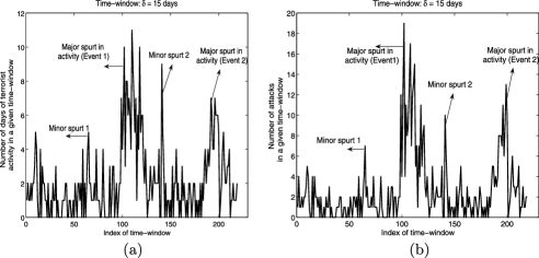
Figure 1: (a) Number of days of terrorist activity, and (b) Total number of attacks in a $\delta$-day time window as a function of time for FARC ($\delta=15$ days). The key geopolitical events in this period are also marked.

2 Preliminaries

2.1 Qualitative features of activity profile

A typical example of the activity profile is presented in Figure 1 where the number of days of terrorist activity in a $\delta=15$ day time window and the total number of attacks within the same time window are plotted as a function of time. The focus of this example is Fuerzas Armadas Revolucionarias de Colombia (FARC), studied in Section 5.1. The data for Figure 1 is obtained from the RDWTI and corresponds to incidents over the nine-year period from 1998 to 2006. From Figure 1 and a careful study of the activity profile of many terrorist groups from similar databases, we highlight some of the important features of terrorism data that impact modeling:

• Temporal ambiguity: The exact instance (time) of occurrence of a terrorism incident is hard to pinpoint. This is because accounts of most terrorist events are from third-party sources. Thus, the granularity of incident reportage (i.e., the time scale on which incidents are reported) that is most relevant is discrete, typically days.

• Attributional ambiguity: Further, in many of the databases, there exists an ambiguity in attributing a certain terrorism incident to a specific group when multiple groups contest on the same geographical turf. Some of this ambiguity can be resolved by attributing an incident to a specific group based on the attack signature (attack target type, operational details, strategies involved, etc.). However, this is an intensive manual exercise and there is necessarily a certain ambiguity in this resolution.

• Data sparsity: Despite the recent surge in media attention on trans-national terrorist activities and insurgencies, terrorism incidents are “rare” (from the perspective of model learning) even for some of the most active terrorist groups. For example, the data in Figure 1 corresponds to 604 incidents over a nine-year period leading to an average of $\approx\!1.29$ incidents per week. While a case can be made that these databases report only a subset of the true activity, the fact that significant amount of resources have to be invested by the terrorist group for every new incident acts as a natural dampener toward more attacks.

These three features make a strong case for parsimonious models for the activity profile of terrorist groups. Further, any good model should be robust to a small number of errors in terms of mislabeled data and missing data supplied from other terrorism incident databases.

2.2 Prior work

The activity profile of a terrorist group can be modeled as a discrete-time stochastic process. Let the first and last day of the time period of interest be denoted as Day $1$ and Day ${\mathcal{N}}$, respectively. Let $M_{i}$ denote the number of terrorism incidents on the $i$th day of observation, $i=1,\ldots,{\mathcal{N}}$. Note that $M_{i}$ can take values from the set $\{0,1,2,\ldots\}$ with $M_{i}=0$ corresponding to no terrorist activity on the $i$th day of observation. On the other hand, there could be multiple terrorism incidents corresponding to independent attacks on a given day, reflecting a high level of coordination between various subgroups of the group. Let ${\mathcal{H}}_{i}$ denote the history of the group’s activity till day $i$. That is, ${\mathcal{H}}_{i}=\{M_{1},\ldots,M_{i}\},i=1,2,\ldots,{\mathcal{N}}$ with ${\mathcal{H}}_{0}=\varnothing$. The point process model is complete if $\mathsf{P}(M_{i}=r|{\mathcal{H}}_{i-1})$ is specified as a function of ${\mathcal{H}}_{i-1}$ for all $i=1,\ldots,{\mathcal{N}}$ and $r=0,1,2,\ldots.$

We noted in Section 1 that prior work on models for the activity profile fall under one of three categories. In the time-series techniques pioneered by Enders and Sandler (2000), a nonlinear trend component, a seasonality (cyclic) component and a stationary component are fitted to the time-series data of worldwide terrorism incidents. In particular, the following model-fit is proposed for $\{M_{i}\}$:

$$\sum_{i\in\Delta_{q}}M_{i}=\sum_{j=0}^{n}\alpha_{j}q^{j}+\beta\sin(\omega q+\phi)+\mu_{q},$$

where $\Delta_{q}$ denotes the period corresponding to the $q$th quarter in the period of observation and $\{n,\alpha_{0},\ldots,\alpha_{n},\beta,\omega,\phi,\mathsf{Var}(\mu_{q})\}$ are parameters to be optimized over some parameter space. This modeling effort results in an eight-parameter model (4 for the trend component, 3 for the seasonality component and a variance parameter for the stationary component) which is then used to identify a rough $4$ and $1/2$-year cycle in terrorism events. Further, a nonlinear trend and seasonality component ensures that trends in terrorism cannot be predicted, thus explaining the observed boom and bust cycles in terrorist activity. Alternately, a TAR model that switches from one auto-regressive process to another with the switches corresponding to key geopolitical events is studied in Enders and Sandler (2002).

On the other hand, the SEHM of Porter and White (2012) is described as

$$\mathsf{P}(M_{i}=r|{\mathcal{H}}_{i-1})=\cases{e^{-(B_{i}+\operatorname{SE}_{i}({\mathcal{H}}_{i-1}))},&\quad$r=0,$\vspace*{2pt}\cr\displaystyle\frac{r^{-s}}{\zeta(s)}\cdot\bigl{(}1-e^{-(B_{i}+\operatorname{SE}_{i}({\mathcal{H}}_{i-1}))}\bigr{)},&\quad$r\geq 1,$}$$ (1)

where $B_{i}$ is a baseline process, and $\operatorname{SE}_{i}(\cdot)$ is the self-exciting component given as

$$\operatorname{SE}_{i}({\mathcal{H}}_{i-1})=\sum_{j:j<i,M_{j}>0}\alpha_{j}g(i-j)$$

for an appropriate choice of decay function $g(\cdot)$ and influence parameters $\{\alpha_{j}\}$. On the other hand, $s\in(1,\infty)$ is an appropriately chosen parameter of the zeta distribution, and $\zeta(s)=\sum_{n=1}^{\infty}n^{-s}$ is the Riemann-zeta function. While a constant $s$ parameter leads to the simplest modeling framework, $s$ can in general be driven by another self-exciting process. A class described by eight parameters is studied in Porter and White (2012) and it is shown that a four-parameter model optimizes an AIC metric for terrorism data from Indonesia/Timor-Leste over the period from 1994 to 2007. This model is shown to accurately capture terrorism data (especially the extreme outliers such as days with $36,11$ and $10$ attacks). The heavy-tailed zeta distribution is also explored in Clauset, Young and Gleditsch (2007) for modeling extremal terrorist events.

3 Proposed model for the activity profile

While the above set of models capture terrorism data, we now propose a competing alternate framework based on HMMs. Our proposed framework is based on the following simplifying hypotheses:

• Hypothesis 1: The activity profile of a terrorist group $\{M_{i},i=1,\ldots,{\mathcal{N}}\}$ depends only on certain states ($\mathbf{S}_{i}$) in the sense that the current activity is conditionally independent of the past activity/history of the group given the current state:

  $$\mathsf{P}(M_{i}|{\mathcal{H}}_{i-1},\mathbf{S}_{i})=\mathsf{P}(M_{i}|\mathbf{S}_{i}),\qquad i=1,2,\ldots.$$

  In other words, these states completely capture the facets from the past history of the group in determining the current state of activity. While attaching specific meanings to $\mathbf{S}_{i}$ is not the focus of this paper, an example in this direction is the postulate by Cragin and Daly (2004) that the Intentions and the Capabilities of a group could serve as these states.

• Hypothesis 2: The dynamics of terrorism are well understood if the underlying states $\{\mathbf{S}_{i}\}$ are known. However, in reality, $\mathbf{S}_{i}$ cannot be observed directly and we can only make indirect inferences about it by observing $\{M_{j},j=1,\ldots,i\}$. To allow inferencing of $\mathbf{S}_{i}$, we propose a $d$-state model that captures the dynamics of the group’s latent states over time. That is, $\mathbf{S}_{i}\in\{0,1,\ldots,d-1\}$ with each distinct value corresponding to a different level in the underlying attributes of the group. Further, we penalize frequent state transitions in the terrorist group dynamics by constraining $\mathbf{S}_{i}$ to be fixed over a block (time window) of $\delta$ days, where $\delta$ is chosen appropriately based on the group dynamics.

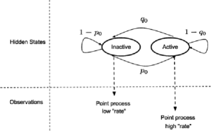
Figure 2: A simple $d=2$ state HMM for the activity of a terrorist group.

A typical illustration of this framework with $d=2$ is provided in Figure 2, where the state over the $n$th time window ($\Delta_{n},n=1,2,\ldots,K$) corresponding to $\Delta_{n}=\{(n-1)\delta+1,\ldots,n\delta\}$ and $K=\lceil\frac{{\mathcal{N}}}{\delta}\rceil$ is given as

$$\mathbf{S}_{i}|_{i\in\Delta_{n}}=s_{n},\qquad s_{n}\in\{0,1\}.$$

In the Inactive state ($s_{n}=0$), the underlying $M_{i}$ form a low-“rate” point process, whereas in the Active state ($s_{n}=1$), the $M_{i}$ form a high-“rate” point process. Thus, a state transition from $s_{n-1}=0$ to $s_{n}=1$ indicates a spurt in the activity of the group, whereas an opposite change indicates a downfall in the activity. This evolution in the states of the group is modeled by a state transition probability matrix $\mathbf{P}=\{\mathsf{P}_{ij}\}$, where

$$\mathbf{P}=\left[\matrix{1-p_{0}&p_{0}\vspace*{2pt}\cr q_{0}&1-q_{0}}\right]$$

with $\mathsf{P}_{ij}\triangleq\mathsf{P}(s_{n}=j|s_{n-1}=i),i,j\in\{0,1\}$. In general, there exists a trade-off between accurate modeling of the group’s latent attributes (larger $d$ is better for this task) versus estimating more model parameters (smaller $d$ is better). While attention in the sequel will be restricted to the $d=2$ setting because of the implementation ease of the proposed approaches in this setting, these approaches can be easily extended to a general $d$-state setting.

To model the observations in either state [i.e., $\mathsf{P}(M_{i}|\mathbf{S}_{i}=j),j=0,1$], a geometric density can be motivated with the following hypothetical scenario. Consider a setting where the group has infinite resources and orchestrates $M_{i}$ attacks on the $i$th day till the success of a certain short-term policy objective can be declared. Every additional attack contributes equally to the success of this objective and, as long as the group’s objective has not been met, attaining this objective in the future is not dependent on the past attacks. In other words, the group remains memoryless (or is oblivious) of its past activity and continues to attack with the same pattern as long as its objective remains unmet. A slight modification in the group dynamics that assumes that a group resistance/hurdle needs to be overcome before this modus operandi kicks in leads to a hurdle-based geometric model for $\{M_{i}\}$.

While these strategies are theoretically motivated and at best may describe a specific group, other groups could adopt different strategies. In fact, strategies could also change with time. Thus, a certain model could make more sense for a given terrorist group than other models. In our subsequent study, we consider the following one-parameter models with support on the nonnegative integers: Poisson, shifted zeta, and geometric. We also consider the following two-parameter models: Pòlya, (nonself-exciting) hurdle-based zeta, and hurdle-based geometric. Of these six models, the geometric and the hurdle-based geometric allow simple recursions for estimates of model parameter(s) via the Baum–Welch algorithm, while the shifted zeta and the hurdle-based zeta distributions allow heavy tails; see supplementary material, Part A [Raghavan, Galstyan and Tartakovsky (2013a)]. Further details on these models, such as the associated probability density function, log-likelihood function, Maximum Likelihood (ML) estimate of the model parameters and a formula for the AIC, are also provided in Raghavan, Galstyan and Tartakovsky (2013a). The study of fits of these models to specific terrorist groups is undertaken in Section 6.2.

4 Detecting spurts and downfalls in activity profile

We are interested in solving the inference problem:

$$\widehat{s}_{n}|_{n=1,\ldots,K}=\mathop{\arg\max}_{s_{1},\ldots,s_{K}\in\{0,1\}^{K}}\mathsf{P}\bigl{(}\mathbf{S}_{i}=s_{n},i\in\Delta_{n}|\{M_{j},j=1,\cdots,{\mathcal{N}}\}\bigr{)}.$$ (2)

In particular, we are interested in identifying state transitions that correspond to either a spurt or a downfall in activity.

Since we are interested in tracking changes in the latent attributes of the group, we focus on an observation sequence that captures the resilience of the group and another that reflects the level of coordination in the group [Santos (2011), Lindberg (2010)]. In particular, the ability of a group to sustain terrorist activity over a number of days reflects its capacity to rejuvenate itself from asset (manpower, material and skill-set) losses. And the ability of the group to launch multiple attacks over a given time period reflects its capacity to coordinate these assets necessary for simultaneous action often over a wide geography. That is, mathematically speaking, the focus is on: (i) $X_{n}$, the number of days of terrorist activity, and (ii) $Y_{n}$, the total number of attacks, both within the $\delta$-day time window $\Delta_{n}$:

$$X_{n}=\sum_{i\in\Delta_{n}}\mathbh{1}\bigl{(}\{M_{i}>0\}\bigr{)};\qquad Y_{n}=\sum_{i\in\Delta_{n}}M_{i},\qquad n=1,2,\ldots,$$

where $\mathbh{1}(\cdot)$ denotes the indicator function of the set under consideration. Note that $Y_{n}/\delta$ is the average number of attacks per day and, thus, $Y_{n}$ is a reflection of the intensity of attacks launched by the group. In general, $X_{n}$ is more indicative of resilience in the group, whereas $Y_{n}$ captures the level of coordination better.

To build a model-driven detection strategy, we now develop a probabilistic model for $X_{n}$ and $Y_{n}$. For this, we leverage the rare nature of terrorism to hypothesize that most terrorist groups tend to be in an Inactive state for far longer than in an Active state. Thus, it is reasonable to assume that $\mathbf{S}_{i}=0$ for long stretches of time and $\gamma_{0}\approx 0$, where

$$\gamma_{j}\triangleq\mathsf{P}(M_{i}>0|\mathbf{S}_{i}=j),\qquad j=0,1.$$ (3)

Over such a long stretch where $\mathbf{S}_{i}=0$, an elementary consequence of (3) is that $X_{n}$ is a binomial random variable with parameters $\delta$ and $\gamma_{0}$:

$$\mathsf{P}(X_{n}=k)=\pmatrix{\delta\cr k}\cdot(\gamma_{0})^{k}\cdot(1-\gamma_{0})^{\delta-k}.$$

If $\delta$ is sufficiently large (typical values used in subsequent case studies are $\delta=15$ to $30$ days) so that the binning/edge effects can be neglected, $X_{n}$ can be well approximated by a Poisson random variable with rate parameter $\delta\gamma_{0}$. In fact, we have the following bound [Teerapabolarn (2012), Corollary 3.2] on the approximability of the binomial distribution by Poisson for $k=0,\ldots,\delta$:

$$\bigl{|}\mathsf{P}_{\mathsf{Bin}}(X_{n}=k)-\mathsf{P}_{\mathsf{Poi}}(X_{n}=k)\bigr{|}\leq\min\biggl{(}1-e^{-\delta\gamma_{0}},\frac{\delta\gamma_{0}}{k}\biggr{)}\cdot\gamma_{0}\approx 0.$$ (4)

Equivalently, let $T_{k},k=1,2,\ldots$ denote the time to the $k$th day of terrorist activity (with $T_{0}$ set to $T_{0}=0$). Then, $\Delta T_{k}=T_{k}-T_{k-1}$ denotes the time to the subsequent day of activity (inter-arrival duration) and $\Delta T_{k}$ is approximately exponential with mean $1/\gamma_{0}$. While a similar reasoning suggests that $\Delta T_{k}$ in the Active state is exponential with mean $1/\gamma_{1}$, this fit is bound to be good only in the first-order sense because a terrorist group is expected to stay in the Active state for relatively shorter durations and $\gamma_{1}\gg\gamma_{0}$. Rephrasing the above conclusions, a discrete-time Poisson process model is a good model for the days of terrorist activity, especially in the Inactive state.

Under the same assumptions (as above), in the Inactive state, $Y_{n}$ can be rewritten as

$$Y_{n}=\sum_{i\in{\mathcal{A}}_{n}}M_{i},$$

where ${\mathcal{A}}_{n}\subset\Delta_{n}$ is the set of days of activity in $\Delta_{n}$ with $|{\mathcal{A}}_{n}|=X_{n}$. Thus, $Y_{n}$ can be approximated as a compound Poisson random variable [Cox and Isham (1980)] whose density is expressed in terms of the density function of $M_{i}$. For example, if $M_{i}$ is independent and identically distributed (i.i.d.) as geometric with $\mathsf{P}(M_{i}=k|\mathbf{S}_{i}=0)=(1-\gamma_{0})\cdot(\gamma_{0})^{k},k\geq 0$, a simple computation [see Raghavan, Galstyan and Tartakovsky (2013a)] shows that

$$\mathsf{P}(Y_{n}=r)=(1-\gamma_{0})^{\delta}\cdot(\gamma_{0})^{r}\cdot\pmatrix{\delta+r-1\cr r},\qquad r\geq 0.$$

Similarly, the joint density of $(X_{n},Y_{n})$ can be written as

$$\mathsf{P}(X_{n}=k,Y_{n}=r)=(1-\gamma_{0})^{\delta}(\gamma_{0})^{r}\cdot\pmatrix{\delta\cr k}\cdot\pmatrix{r-1\cr r-k},\qquad r\geq k,$$

where the condition $r\geq k$ ensures that at least one attack occurs on a day of activity. With the more general hurdle-based geometric model, where

$$\mathsf{P}(M_{i}=k|\mathbf{S}_{i}=0)=\cases{1-\gamma_{0},&\quad$k=0,$\vspace*{2pt}\cr\gamma_{0}(1-\mu_{0})\cdot(\mu_{0})^{k-1},&\quad$k\geq 1,$}$$

the joint density is given as

$$\mathsf{P}(X_{n}=k,Y_{n}=r)=\pmatrix{\delta\cr k}\pmatrix{r-1\cr r-k}\cdot(1-\gamma_{0})^{\delta-k}(\gamma_{0})^{k}\cdot(1-\mu_{0})^{k}(\mu_{0})^{r-k},$$

$$\eqntext{r\geq k.}$$ (5)

Replacement of $\gamma_{0}$ and $\mu_{0}$ with $\gamma_{1}$ and $\mu_{1}$ in the Active state works subject to the same issues/constraints as stated earlier.

We now propose a strategy that exploits the underlying HMM structure to detect changes in group dynamics. For this, we treat as observations $\{X_{n}\}$, $\{Y_{n}\}$ and the joint sequence $\{(X_{n},Y_{n})\}$ under different modeling assumptions on $\{M_{i}\}$. We first apply the classical HMM formulation [Rabiner (1989)] where the Baum–Welch algorithm is used to learn the parameters that determine the density function of the observations. For the Baum–Welch algorithm to converge to a local maximum (with respect to the log-likelihood function) in the parameter space, a sufficient condition is that the density function of the observation be log-concave [Rabiner (1989), Section IVA, page 267]. Under the i.i.d. geometric and hurdle-based geometric models for $\{M_{i}\}$, it is established in Raghavan, Galstyan and Tartakovsky (2013a) that all the three density functions are log-concave. Further, an iterative update for the parameter estimates is also established under these two models. With the converged Baum–Welch parameter estimates as the initialization, the Viterbi algorithm is then used to estimate the most probable state sequence given the observations. The output of the Viterbi algorithm is a state estimate for the period of interest

$$\bigl{\{}\mathbf{S}_{i}=\widehat{s}_{n}\in\{0,1\}\ \mathrm{for}\ \mathrm{all}\ i\in\Delta_{n}\ \mathrm{and}\ n=1,\ldots,K\bigr{\}}.$$

A state estimate of $1$ indicates that the group is Active over the period of interest, whereas an estimate of $0$ indicates that the group is Inactive. Transition between states indicates spurt/downfall in the activity.

While we have developed a model-driven strategy, there is often an interest in approaches that are independent of these parameters, and hence not sensitive to the parameter estimation algorithms or the length of the training period. An alternate approach that does not explicitly learn the underlying model parameters can be developed using the Exponential Weighted Moving-Average (EWMA) filter. Details of this approach and its comparative performance with the HMM-based strategy can be found in the work of Raghavan, Galstyan and Tartakovsky (2012).

5 Case-studies

We now undertake two case studies on the fit of a discrete-time Poisson point process model for the days of terrorist activity. For this, we classify terrorist activities as reported in the RDWTI and GTD that catalogue activities by different groups across the world [LaFree and Dugan (2007), RDWTI].

5.1 FARC

We start with FARC, a Marxist-Leninist terrorist group active over a large area in Colombia and its neighborhood. We study the activities of FARC over the nine-year time period from 1998 to 2006. This period covers a total of 604 terrorist incidents in the RDWTI with a yearly breakdown of 44 incidents in 1998, 18 in 1999, 45 in 2000, 27 in 2001, 217 in 2002, 57 in 2003, 33 in 2004, 66 in 2005 and 97 in 2006, respectively. The reasons why FARC and the 1998 to 2006 time period have been chosen for our study are provided in supplementary material, Part B [Raghavan, Galstyan and Tartakovsky (2013b)].

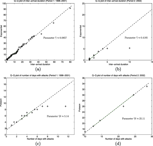
Figure 3: Q–Q plots of duration between days of terrorist activity with respect to a theoretical exponential random variable for the period from: (a) 1998 to 2001 corresponding to normal terrorist activity, and (b) 2002 corresponding to a spurt in terrorist activity. Q–Q plots of number of days of terrorist activity over a $\delta=60$ day time window with respect to a theoretical Poisson random variable for the same two scenarios are presented in (c) and (d).

As explained in Section 4, the activity profile of FARC can be modeled as a discrete-time sampled Poisson point process. In Figure 3, we test the fit of this model by studying: (i) the Quantile–Quantile (Q–Q) plots comparing the sample inter-arrival duration between consecutive days of terrorist activity and an exponential random variable with an appropriately-defined rate parameter ($\widehat{\gamma}$), and (ii) the Q–Q plots comparing the number of days of terrorist activity over a time window of $\delta$ days and a Poisson random variable with parameter $\delta\widehat{\gamma}$. For both sets of Q–Q plots, we consider two scenarios: the first (the 1998 to 2001 period) corresponding to a period of “normal” terrorist activity, and the second (the 2002 period) corresponding to a spurt in terrorist activity.

Figures 3(a) and (b) compare the Q–Q plots of the sample inter-arrival duration under these two scenarios with an exponential random variable. The rate parameter used for the exponential is

$$\widehat{\gamma}=\frac{1}{\mathsf{E}[\Delta T_{k}]},$$ (6)

where $\mathsf{E}[\Delta T_{k}]$ is the sample mean of the inter-arrival duration over the considered period. From Figure 3, we note that both in periods of normal as well as a spurt in activity, the Q–Q plot is nearly linear with a few sample outliers in the tails. These outliers indicate that an exponential model for inter-arrival duration is not accurate because of the heavy tails. Nevertheless, to a first-order, an exponential random variable serves as a good fit for the inter-arrival durations. Our numerical study leads to the following estimates for $\gamma_{\bullet}$: (a) $\widehat{\gamma}\approx 0.0857$, (b) $\widehat{\gamma}\approx 0.4185$, suggesting that a spurt in activity is associated with an increase in the rate parameter. Similarly, in Figures 3(c) and (d), we compare the Q–Q plots of the number of days of terrorist activity over a $\delta=60$ day time window under the same scenarios (as above) with a theoretical Poisson random variable of parameter $\delta\widehat{\gamma}=60\widehat{\gamma}$. While we observe some outliers in the tail quantiles, a Poisson random variable seems to be a good first-order fit for the number of days of terrorist activity.

As explained in Section 4, a geometric model is assumed for $\{M_{i}\}$ and the Baum–Welch algorithm is used to learn the underlying $\gamma_{j}$ with $\{X_{n}\}$, $\{Y_{n}\}$ and $\{(X_{n},Y_{n})\}$ over a given $\delta$-day time window as training data. Specifically, Table 1 summarizes the parameter estimates for different $\delta$ values when $\{(X_{n},Y_{n})\}$ is used as a training set. It is to be noted that the learned parameter values remain stable across a large range of $\delta$ ($1$ to $30$ days) values. The performance of the Baum–Welch algorithm is also robust to both the length of the training set as well as the initialization. Further, the parameter values also remain essentially independent of whether $\{X_{n}\}$, $\{Y_{n}\}$ or $\{(X_{n},Y_{n})\}$ is used for training. For example, with $\delta=15$ and $\{(X_{n},Y_{n})\}$ as training data, the parameter values learned are $\widehat{\gamma}_{0}=0.0924$ and $\widehat{\gamma}_{1}=0.3605$, whereas with $\{X_{n}\}$, these values are $\widehat{\gamma}_{0}=0.0941$ and $\widehat{\gamma}_{1}=0.3861$. This observation is not entirely surprising since $\{M_{i}\}$ is assumed to come from a one-parameter model family and conditioned on one of the two variables ($X_{n}$ or $Y_{n}$), the other variable adds no significant new information about the model parameter.

Table 1: State classification of FARC with the geometric and hurdle-based geometric models and $\{(X_{n},Y_{n})\}$ as observations for different time window periods ($\delta$)

	Parameters learned
$\bolds{\delta}$ (in days)	$\bolds{\widehat{\gamma}_{0}}$	$\bolds{\widehat{\gamma}_{1}}$	Length of training set ($\bolds{N}$ time windows)	No. of Active states ($\bolds{\mathsf{N}_{\mathsf{spurt}}}$ time windows)	Fractional activity $\bolds{(\mathsf{f}=\frac{\mathsf{N}_{\mathsf{spurt}}\cdot\delta}{{\mathcal{N}}})}$
$1$	$0.0924$	$0.3597$	$3286$	$483$	$0.1469$
$5$	$0.0919$	$0.3584$	0$657$	$140$	$0.2130$
$7$	$0.0924$	$0.3598$	0$469$	0$89$	$0.1895$
$10$	$0.0911$	$0.3568$	0$328$	0$73$	$0.2221$
$15$	$0.0924$	$0.3605$	0$219$	0$46$	$0.2099$
$25$	$0.0908$	$0.3592$	0$131$	0$26$	$0.1977$
$30$	$0.0930$	$0.3593$	0$109$	0$20$	$0.1825$

	Parameters learned
$\bolds{\delta}$ (in days)	$\bolds{\widehat{\gamma}_{0}}$	$\bolds{\widehat{\mu}_{0}}$	$\bolds{\widehat{\gamma}_{1}}$	$\bolds{\widehat{\mu}_{1}}$	Length of training set ($\bolds{N}$ time windows)	No. of Active states ($\bolds{\mathsf{N}_{\mathsf{spurt}}}$ time windows)	Fractional activity $\bolds{(\mathsf{f}=\frac{\mathsf{N}_{\mathsf{spurt}}\cdot\delta}{{\mathcal{N}}})}$
$1$	$0.0950$	$0.0752$	$0.3982$	$0.3083$	$3286$	$484$	$0.1472$
$5$	$0.0942$	$0.0730$	$0.3934$	$0.3066$	0$657$	$140$	$0.2130$
$7$	$0.0949$	$0.0742$	$0.3956$	$0.3081$	0$469$	0$87$	$0.1853$
$10$	$0.0936$	$0.0724$	$0.3891$	$0.3044$	0$328$	0$71$	$0.2160$
$15$	$0.0958$	$0.0759$	$0.4019$	$0.3103$	0$219$	0$42$	$0.1917$
$25$	$0.0934$	$0.0738$	$0.3957$	$0.3046$	0$131$	0$26$	$0.1977$
$30$	$0.0954$	$0.0794$	$0.3966$	$0.3073$	0$109$	0$20$	$0.1825$

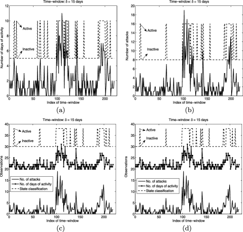
Figure 4: State classification via Viterbi algorithm with the geometric model for $\{M_{i}\}$; Observations being (a) $\{X_{n}\}$, (b) $\{Y_{n}\}$ and (c) $\{(X_{n},Y_{n})\}$ with parameters learned by Baum–Welch algorithm. (d) State classification with the hurdle-based geometric model for the observation sequence $\{(X_{n},Y_{n})\}$.

The converged Baum–Welch parameter estimates are then used to initialize the Viterbi algorithm to obtain the most probable state sequence for FARC. Figures 4(a)–(c) illustrate the state classification for a $\delta=15$ day time window with $\{X_{n}\}$, $\{Y_{n}\}$ and $\{(X_{n},Y_{n})\}$ as observations. As can be seen from Figure 4, the state classification approach detects even small and nonpersistent changes. Further, the Viterbi algorithm declares $51$ and $46$ of the $219$ time windows as Active with $\{X_{n}\}$ and $\{Y_{n}\}$, respectively, whereas the joint sequence $\{(X_{n},Y_{n})\}$ results in the same classification as $\{Y_{n}\}$. Table 1 summarizes the number of time windows classified as Active for different $\delta$ values with $\{(X_{n},Y_{n})\}$ as observations. This study also suggests that $\delta=10$ to $15$ with the HMM approach optimally trading off the twin objectives of detecting minor spurts in the activity profile of FARC (larger $\mathsf{N}_{\mathsf{spurt}}$) as well as minimizing the number of Active state classifications that require further attention (smaller fractional activity $\mathsf{f}$).

We now consider a more general two-parameter hurdle-based geometric model for $\{M_{i}\}$ that potentially allows the joint sequence $\{(X_{n},Y_{n})\}$ to result in better inferencing on the states than either $\{X_{n}\}$ or $\{Y_{n}\}$. As before, the Baum–Welch algorithm is used to learn the underlying parameters with different values of $\delta$ and $\{(X_{n},Y_{n})\}$ as training data. Table 1 summarizes these parameter estimates and, as was the case earlier, it can be seen that the estimates remain stable across $\delta$. The parameter estimates are then used with the Viterbi algorithm to infer the most probable state sequence [see Figure 4(d) for state classification in the $\delta=15$ setting]. While Figure 4(d) and Table 1 show that the classification with the hurdle-based model agrees with the simpler geometric model for many $\delta$ values, in the setting of interest ($\delta=7$ to $15$ days), the hurdle-based model is more conservative in declaring an Active state. The four time windows of disagreement between the hurdle-based geometric and geometric models for $\delta=15$ correspond to the boundary of minor spurts (time windows $11$, $64$, $191$ and $204$), where the hurdle-based model is more conservative in declaring an Active state, whereas the geometric model is trigger-happy.

5.2 Shining Path

The second case study is the activity profile of Sendero Luminoso (more popularly known as Shining Path), a terrorist group in Peru. With a focus on the sixteen-year period between 1981 and 1996, the RDWTI reports a total of 163 incidents with a yearly breakdown of 10 incidents in 1981, 7 in 1982, 10 in 1983, 7 in 1984, 3 in 1985, 12 in 1986, 19 in 1987, 7 in 1988, 18 in 1989, 10 in 1990, 31 in 1991, 10 in 1992, 14 in 1993, 2 in 1994, 2 in 1995 and 1 in 1996. The choice of Shining Path and the 1981 to 1996 time period are motivated in supplementary material, Part B [Raghavan, Galstyan and Tartakovsky (2013b)].

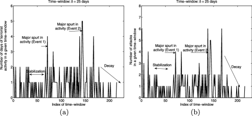
Figure 5: (a) Number of days of terrorist activity, and (b) Total number of attacks in a $\delta=25$ day time window as a function of time for Shining Path.

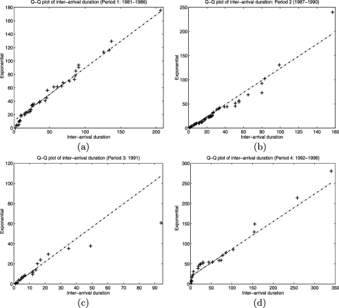
Figure 6: Q–Q plots of duration between days of terrorist activity with respect to a theoretical exponential distribution for the period from: (a) 1981 to 1986, (b) 1987 to 1990, (c) 1991, and (d) 1992 to 1996 corresponding to different stages of evolution of Shining Path.

In Figure 5, we plot the number of days of terrorist activity and the total number of attacks over a $\delta=25$ day time window. In Figure 6, we test the fit of inter-arrival duration between successive days of terrorist activity with respect to an exponential random variable with parameter $\widehat{\gamma}$ estimated as in (6). As noted in supplementary material, Part B [Raghavan, Galstyan and Tartakovsky (2013b)], the evolution of Shining Path can be partitioned into four distinct phases. The inter-arrival duration in each phase can be distinctly modeled as an exponential random variable and Figure 6 shows that this partitioning is reasonable. As in the case with FARC, the exponential random variable is a good first approximation, as the tails are not well modeled with this random variable. Our numerical study leads to the following estimates for $\gamma_{\bullet}$ in the four phases: (a) $\widehat{\gamma}\approx 0.0211$, (b) $\widehat{\gamma}\approx 0.0344$, (c) $\widehat{\gamma}\approx 0.0755$, (d) $\widehat{\gamma}\approx 0.0158$.

As elucidated with the FARC data set, the data corresponding to Shining Path is studied in the following experiment. Using the HMM approach with the hurdle-based geometric model described in Section 4, the Baum–Welch algorithm results in parameter estimates as in Table 2 for different values of $\delta$. State classification via the Viterbi algorithm using these estimates results in an Active/Inactive classification for Shining Path, for example, Figure 7 displays a typical classification for $\delta=25$. It is important to note that while four distinct phases are identified in the evolution of Shining Path, only a $d=2$-state HMM is studied here. For the purpose of spurt/downfall detection, even this coarse model is sufficient. As can be seen with FARC data, even small and nonpersistent changes are detected by the HMM approach, further confirming its usefulness.

Table 2: State classification of Shining Path with the hurdle-based geometric model and $\{(X_{n},Y_{n})\}$ as observations for different time window periods ($\delta$)

	Parameters learned
$\bolds{\delta}$ (in days)	$\bolds{\widehat{\gamma}_{0}}$	$\bolds{\widehat{\mu}_{0}}$	$\bolds{\widehat{\gamma}_{1}}$	$\bolds{\widehat{\mu}_{1}}$	Length of training set ($\bolds{N}$ time windows)	No. of Active states ($\bolds{\mathsf{N}_{\mathsf{spurt}}}$ time windows)	Fractional activity $\bolds{(\mathsf{f}=\frac{\mathsf{N}_{\mathsf{spurt}}\cdot\delta}{{\mathcal{N}}})}$
$20$	$0.0262$	$0.1026$	$0.1000$	$0.6667$	$268$	$69$	$0.2575$
$25$	$0.0264$	$0.1019$	$0.0800$	$0.6667$	$215$	$35$	$0.1628$
$28$	$0.0264$	$0.1019$	$0.0714$	$0.6667$	$192$	$15$	$0.0781$
$30$	$0.0262$	$0.1026$	$0.0667$	$0.6667$	$179$	$14$	$0.0782$
$32$	$0.0202$	$0.0703$	$0.1072$	$0.2255$	$168$	$38$	$0.2262$

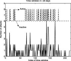
Figure 7: State classification for Shining Path data ($\delta=25$ days).

6 Revisiting some of the modeling issues

We now revisit some of the modeling issues that shed further light on development of good models for the activity profile of terrorist groups.

6.1 Clustering of attacks

A central premise in terrorism modeling is that the current activity of a terrorist group is influenced by its past activity. One consequence of this premise is that the attacks perpetrated by the group are clustered [Midlarsky (1978), Midlarsky, Crenshaw and Yoshida (1980)]. Ripley’s $K(\cdot)$ function is a statistical tool for measuring the degree of clustering (aggregatedness) or inhibition (regularity) in a point process as a function of inter-point distance [Diggle (2003)]. Specifically, if $\lambda$ is the intensity of the point process, $\lambda K(h)$ is the expected number of other points within a distance $h$ of a randomly chosen point of the process:

$$K(h)\triangleq\frac{1}{\lambda}\cdot\mathsf{E}[\mbox{Number of other points within distance $h$}$$

$$\hskip 125.0pt\mbox{of a randomly chosen point}].$$

Expressions for $K(h)$ can be derived for a number of stationary point process models [Dixon (2002)]. For example, in the case of a one-dimensional/temporal point process that is completely random (where points are distributed uniformly and independently in time), it can be shown that $K(h)=2h$. A two-dimensional complete random spatial point process leads to $K(h)=\pi h^{2}$. In the context of an activity profile, $K(h)$ can be estimated as

$$\widehat{K}(h)=\frac{1}{\widehat{\lambda}\cdot N}\sum_{i}\sum_{j\neq i}\mathbh{1}\bigl{(}|t_{i}-t_{j}|\leq h\bigr{)}=\frac{1}{(\widehat{\lambda})^{2}\cdot{\mathcal{N}}}\sum_{i}\sum_{j\neq i}\mathbh{1}\bigl{(}|t_{i}-t_{j}|\leq h\bigr{)},$$ (7)

where $t_{i}$ is the $i$th day of activity, $N$ is the number of attacks in the observation period of ${\mathcal{N}}$ days (i.e., $[t_{1},\ldots,t_{N}]=[\mathrm{Day}1,\ldots,\mathrm{Day}{\mathcal{N}}]$), and $\widehat{\lambda}=\frac{N}{{\mathcal{N}}}$ is an estimate of the intensity (rate) of the process. Significant deviations of $\widehat{K}(h)$ from $2h$ indicate that the hypothesis of complete randomness becomes untenable with observed data and more confidence is reposed on clustering [if $\widehat{K}(h)\gg 2h$] or inhibition [if $\widehat{K}(h)\ll 2h$].

While the definition in (7) assumes a homogenous point process, extensions to an inhomogenous point process have also been proposed [Baddeley, Møller and Waagepetersen (2000), Veen and Schoenberg (2006)], where the point process is re-weighted by the reciprocal of the nonconstant intensity function to offset the inhomogeneity. Further, to compensate for edge effects due to points outside the observation period being left out in the numerator of (7), various edge-correction estimators have also been proposed in the literature. Combining these two facets, we have the following estimator for $K(h)$:

$$\widehat{K}(h)=\frac{1}{{\mathcal{N}}}\sum_{i}\sum_{j\neq i}\frac{\mathbh{1}(|t_{i}-t_{j}|\leq h)}{\widehat{p}_{i}\widehat{p}_{j}w_{ij}},$$ (8)

where $\widehat{p}_{i}$ is the estimated probability of at least one attack on $t_{i}$. In this work, we use an edge-correction factor $w_{ij}$ due to Ripley [Cressie (1991), pages 616–618] which reflects the proportion of the period centered at $t_{i}$ and covering the $j$th day of activity that is included in the observation period:

$$w_{ij}=\cases{1,&$\quad\mathrm{if}\ t_{1}+R\leq t_{i}\leq t_{N}-R,$\vspace*{2pt}\cr\displaystyle\frac{t_{N}-t_{i}+R}{2R},&\quad$\mathrm{if}\ t_{i}>\max(t_{N}-R,t_{1}+R),$\vspace*{2pt}\cr\displaystyle\frac{R+t_{i}-t_{1}}{2R},&\quad$\mathrm{if}\ t_{i}<\min(t_{N}-R,t_{1}+R),$\vspace*{2pt}\cr\displaystyle\frac{t_{N}-t_{1}}{2R},&\quad$\mathrm{if}\ t_{N}-R\leq t_{i}\leq t_{1}+R,$}$$

where $R=|t_{i}-t_{j}|$.

In Figure 8(a), we plot $K(h)-2h$ computed as in (8) for the FARC data set (with and without edge-correction) as a function of the inter-point distance $h$. In line with the observation by Porter and White (2012) for the Indonesia/Timor-Leste data set, the plot here indicates that the FARC data is also clustered since $K(h)-2h\gg 0$, thus motivating the SEHM.

Figure 8: (a) $K(h)$ as a function of inter-point distance $h$ for the activity profile of FARC and under the two states of the HMM, (b) fractional change in state classification relative to addition of missing data from GTD.

The main theme of this work, however, is that clustering is essentially a reflection of state transitions and the activity sub-profile (sub-series) of the group conditioned on a given state value is not clustered. To test this hypothesis, we study the behavior of $K(h)$ for the sub-series from the FARC data set corresponding to the Active and Inactive states as classified by the methodology of Section 5.1. Since the latent states of the group transition back and forth, an Active sub-series is constructed by patching together the group’s activity profile in the Active state with the jump random variable between any two disjoint pieces of the activity profile modeled as Poisson with parameter $\widehat{\lambda}=\frac{N}{{\mathcal{N}}}$. For this sub-series, $K(h)$ is estimated using a formula analogous to (8), where $\widehat{p}_{i}$ and $w_{ij}$ are re-estimated for the sub-series, and ${\mathcal{N}}$ is replaced with ${\mathcal{N}}_{\mathsf{act}}$:

$${\mathcal{N}}_{\mathsf{act}}=\min(\mbox{Number of days in \emph{Active} state, Length of \emph{Active} sub-series}).$$

A confidence interval can also be constructed using the bootstrap technique (resampling from the underlying data distribution). A similar estimation process yields $K(h)$ and the corresponding confidence interval for the Inactive sub-series.

In contrast to the trends for the unclassified activity profile, both the sub-series indicate an inhibitory behavior (mild inhibition for the Active state and stronger inhibition for the Inactive state) in Figure 8(a). Further, $K(h)-2h$ lies within the $95\%$ confidence interval (computed using a $1000$-point resampling) for almost all $h$ values with the Active sub-series and for a significant fraction of $h$ values with the Inactive sub-series. The stronger inhibition in the Inactive state should not be entirely surprising since very few attacks happen in this state. The absence of clustering in the activity profile conditioned on the latent state suggests that the clustering of attacks can also be explained as arising due to different intensity profiles in the different states. Thus, the HMM framework offers a competing approach to explain the clustering of attacks.

Table 3: Histogram of observed number of attacks per day for FARC data with different model fits, $\delta=15$ days

						Hurdle-based	Hurdle-based
No. attacks	Obs.	Poisson	Shifted zeta	Geomet.	Pòlya	textbfzeta	geomet.
(Inactive state)
$0$	$2420$	$2421$	$2470$	$2430$	$2421$	$2420$	$2421$
$1$	$227$	$225$	$144$	$207$	$225$	$229$	$226$
$2$	$9$	$11$	$27$	$18$	$11$	$7$	$10$
$3$	$1$	$0$	$8$	$2$	$0$	$1$	$0$
$4$	$0$	$0$	$4$	$0$	$0$	$0$	$0$
$>4$	$0$	$0$	$4$	$0$	$0$	$0$	$0$
AIC		1690.34	$1772.81$	$1696.74$	$1692.32$	$1692.58$	$1691.86$
Parameter		$0.0933$	$4.105$	$0.0854$	$\widehat{r}_{0}=24.4749$,	$\widehat{\gamma}_{0}=0.0892$,	$\widehat{\mu}_{0}=0.0444$,
Estimate					$\widehat{y}_{0}=0.0038$	$\widehat{y}_{0}=5.10$	$\widehat{\gamma}_{0}=0.0892$
(Active state)
$0$	$384$	$359$	$455$	$404$	$389$	$384$	$384$
$1$	$174$	$202$	$87$	$144$	$160$	$189$	$171$
$2$	$46$	$57$	$33$	$52$	$56$	$31$	$52$
$3$	$19$	$11$	$16$	$19$	$17$	$11$	$16$
$4$	$4$	$1$	$9$	$7$	$6$	$5$	$5$
$>4$	$3$	$0$	$30$	$4$	$2$	$10$	$2$
AIC		$1313.88$	$1416.88$	$1291.73$	$1288.85$	$1308.09$	1287.11
Parameter		$0.5651$	$2.40$	$0.3611$	$\widehat{r}_{1}=1.4834$,	$\widehat{\gamma}_{1}=0.3905$,	$\widehat{\mu}_{1}=0.3090$,
Estimate					$\widehat{y}_{1}=0.2759$	$\widehat{y}_{1}=2.61$	$\widehat{\gamma}_{1}=0.3905$

6.2 Model for observation densities

We now develop simple models for the observation density under the two states. For this, we study the goodness of fit captured by the AIC for several models with support on the nonnegative integers to describe data from FARC. In Table 3, we present the histogram of the number of days with $\ell$ ($\ell=0,1,\ldots$) attacks per day for FARC data. Applying the state classification algorithm described in Section 4 with $\delta=15$, FARC stays in the Inactive state for $2657$ days and in the Active state for $630$ days. Also, presented in the same table are the (rounded-off) expected number of days with $\ell$ attacks for the six models described in supplementary material, Part A, along with the AIC for these model fits. While the corresponding data for $\delta=10$ is not presented here due to space constraints, FARC stays in the Inactive state for $2577$ days and in the Active state for $710$ days in this setting.

The ML parameter estimates for all the six models remain robust as $\delta$ is varied, which is in conformity with the stability of the converged Baum–Welch parameter estimates with $\delta$ (see Tables 1 and 2). Further, from Table 3, in the Inactive state, it is seen that all the models except the shifted zeta result in comparable fits. Specifically, the hurdle-based geometric model differs from the observed histogram in only one day and results in the second lowest AIC value. On the other hand, in the Active state, the hurdle-based geometric model produces the best fit with only the Pòlya model resulting in a comparable fit. In this setting, the one-parameter models overestimate either the tail or the days of no activity, while the hurdle-based zeta produces a heavier tail than what the data exhibits. In fact, the poorest fit in either state is obtained with the shifted zeta suggesting that a heavy tail may not always be necessary. In contrast, the Indonesia/Timor-Leste data studied in Porter and White (2012) exhibits several extreme values (e.g., days with $36,11$ and $10$ attacks) and the authors observe that a self-exciting hurdle-based zeta model captures the heavy tails much better than other models. The FARC data set used here shows a maximum of $7$ attacks per day, whereas the Shining Path data set shows a maximum of $3$ attacks per day. Even simple nonself-exciting models are enough to capture these data sets well.

This study suggests the following:

• If parsimony of the model is of critical importance, the geometric distribution serves as the best one-parameter model with the Poisson/shifted zeta models either under-estimating or overestimating the number of days with no activity in the Active state.

• If parsimony is not a critical issue and the data does not have (or has very few) extreme values, the hurdle-based geometric model serves as the best/near-best model in either state.

• However, if the data has several extreme values [as seen in Porter and White (2012)], the self-exciting hurdle model offers the best model fit, albeit at the expense of learning several model parameters.

6.3 Inter-arrival duration

We now study the efficacy of the HMM framework by testing the goodness of fit of the theoretical exponential random variable with respect to the inter-arrival duration between days of terrorist activity in either state. To avoid estimating the rate parameters of the exponential random variables from the data (which complicates the hypothesis tests), we use the fact from Seshadri, Csorgo and Stephens (1969) that if $y_{1},\ldots,y_{m}$ are i.i.d. exponential random variables (with a given rate parameter), then

$$z_{j}=\frac{\sum_{i=1}^{j}y_{i}}{\sum_{i=1}^{m}y_{i}},\qquad j=1,\ldots,m$$ (9)

are i.i.d. uniformly distributed in $[0,1]$. We then use a Kolmogorov–Smirnov (KS) test to study the fit between the empirical cumulative distribution function (CDF) of $z_{j}$ and the uniform CDF [Durbin (1973)].

The KS test-statistic (denoted as $\mathsf{KS}_{\bullet}$) and the critical value for the test (denoted as $K_{\alpha}$) corresponding to a significance level $\alpha$ and computed using the standard asymptotic formula are given as

$$\mathsf{KS}_{\bullet} = \max_{x}\Biggl{|}\frac{1}{n_{\bullet}}\sum_{i=1}^{n_{\bullet}}\mathbh{1}\bigl{(}z_{i}^{\bullet}\leq x\bigr{)}-x\Biggr{|},$$

$$K_{\alpha} = \sqrt{\frac{-({1}/{2})\log({\alpha}/{2})}{n_{\bullet}}},$$

where $n_{\bullet}$ is the number of samples and $\{z_{i}^{\bullet}\}$ are the transformed samples computed using (9) in either state. The results of applying the KS test to the two states are presented in Table 4. From this table, it is clear that the samples in either state fit the theoretical exponential assumption very accurately with the exponential model rejected in the Active (and Inactive) state(s) if the significance level $\alpha$ exceeds $\alpha>0.3763$ (and $\alpha>0.7905$), respectively.

Table 4: KS test-statistic in the two states for FARC data set

	Active	Inactive
Total number of samples	$245$	$236$
No. of samples with $\Delta T_{k}\leq\beta$	$n_{\mathsf{A}}=234,\beta=15$	$n_{\mathsf{I}}=192,\beta=20$
KS statistic	$0.0597$	$0.0492$
$p$-value	$0.3763$	$0.7905$

In a recent analysis of FARC activities using the MIPT database over the time period 1998 to 2005, Clauset and Gleditsch (2012) hypothesize that the inter-arrival duration between successive days of attacks “decreases consistently, albeit stochastically” with the cumulative number of events FARC has carried out—a measure of the group’s experience. Our initial studies indicate that while this hypothesis holds empirically true for $k\leq 25$ attacks that encompass the period January 1 to June 27, 1998, it consistently increases through the subsequent period lasting till March 10, 2000. Note that this is the precise time period of increased U.S. funding to combat FARC and the drug economy through Plan Colombia [Haugaard, Isacson and Olson (2005)] and a mean increase in the time to the next day of activity indicates an impact of counter-terrorism efforts. The following period through August 13, 2004 indicates a reversed trend of consistent decrease, suggesting that the organizational dynamics of FARC had “adjusted” to the new reality of combat with the establishment. As seen earlier, such distinct changes in the organizational dynamics (associated with spurts and downfalls) are quickly identified by the approaches proposed in this work.

6.4 Robustness of proposed approach to missing data

We now study the robustness of the proposed spurt detection approach in terms of state classification to attacks that are not available in the database. Toward this goal, we treat the FARC data from RDWTI over the 1998 to 2006 period as the baseline data set and add one missing day of activity per year from the GTD in a sequential manner and revisit state classification with the enhanced data set. Specifically, the fraction of missing data added in the $j$th (sequential) step is the ratio of the difference between new and old attacks and the baseline, and is defined as

$$\mathrm{Frac.\ Missing\ Data}(j)\triangleq\frac{\sum_{i=1}^{{\mathcal{N}}}\widetilde{M}_{i}^{j}-M_{i}}{\sum_{i=1}^{{\mathcal{N}}}M_{i}},$$

where $\widetilde{M}_{i}^{j}$ is the number of attacks on the $i$th day with data addition. Applying the state estimation algorithm proposed in Section 4 to this new data set, let $\widehat{s}_{i,j}^{\mathsf{new}}\in\{0,1\}$ denote the estimated state value on the $i$th day ($i=1,\ldots,{\mathcal{N}}$). The fractional change in state classification is then defined as

$$\mathrm{Frac.\ State\ Classification\ Changes}(j)\triangleq\frac{\sum_{i=1}^{{\mathcal{N}}}|\widehat{s}_{i,j}^{\mathsf{new}}-\widehat{s}_{i}|}{{\mathcal{N}}},$$

with $\widehat{s}_{i}$ denoting the state classification on the $i$th day with the baseline data set.

In Figure 8(b), $\mathrm{Frac.}\ \mathrm{Missing}\ \mathrm{Data}(j)$ is plotted as a function of $\mathrm{Frac.}\break\mathrm{State}\mathrm{Classification}\ \mathrm{Changes}(j)$. In general, combining terrorism information from two different databases with a clear dichotomy in terms of data collection standards (criteria for inclusion and noninclusion of events, source material used, etc.) can introduce a systematic bias in terrorism trends. Despite this anomaly, it is clear from Figure 8(b) that the proposed approach is remarkably robust to a small amount of missing data. For example, the addition of an $\approx 5\%$ more data to the baseline data set leads to essentially no changes in state classification with the baseline data set. On the other extreme, big additions of even up to $65\%$ more data result in only an $\approx 10\%$ mismatch in state classifications.

6.5 Comparing the TAR, SEHM and HMM frameworks

It is important to compare the proposed HMM framework with the existing TAR and SEHM frameworks in terms of the models’ explanatory and predictive powers. While this comparison requires a careful study of performance across data sets (and is the subject of ongoing work), we now provide initial results in this direction. We study both models’ ability to explain the times to the subsequent day of activity $\{\Delta T_{1}^{n}\}$ and their ability to predict $\Delta T_{n+1}$ given $\{\Delta T_{1}^{n}\}$. We validate both models with the FARC data set and the Indonesia/Timor-Leste data set studied by Porter and White (2012).

Table 5: Comparison between AIC and SMAPE scores with SEHM and HMM for FARC and Indonesia/Timor-Leste data sets

$\bolds{\mathsf{AIC}}$						$\bolds{\mathsf{SMAPE}}$
$\bolds{\mathsf{FARC}}$			$\bolds{\mathsf{Indonesia/Timor\mbox{-}Leste}}$			$\bolds{\mathsf{FARC}}$			$\bolds{\mathsf{Indonesia/Timor\mbox{-}Leste}}$
$\bolds{n}$	$\bolds{\mathsf{SEHM}}$	$\bolds{\mathsf{HMM}}$	$\bolds{n}$	$\bolds{\mathsf{SEHM}}$	$\bolds{\mathsf{HMM}}$	$\bolds{n}$	$\bolds{\mathsf{SEHM}}$	$\bolds{\mathsf{HMM}}$	$\bolds{n}$	$\bolds{\mathsf{SEHM}}$	$\bolds{\mathsf{HMM}}$
$100$	0$671.68$	0$671.06$	$100$	0$723.78$	0$729.47$	$100$	$46.27\%$	$52.78\%$	$100$	$46.33\%$	$43.32\%$
$200$	$1117.40$	$1112.07$	$165$	$1091.78$	$1116.92$	$150$	$42.95\%$	$35.75\%$	$125$	$45.47\%$	$41.89\%$
$300$	$1521.93$	$1521.36$	$200$	$1283.08$	$1305.27$	$200$	$40.40\%$	$35.61\%$	$150$	$42.84\%$	$38.75\%$
$400$	$2127.55$	$2121.81$	$250$	$1589.43$	$1615.87$	$250$	$40.09\%$	$38.14\%$	$175$	$45.23\%$	$38.00\%$
$450$	$2333.88$	$2327.02$	$300$	$2018.92$	$2041.35$	$300$	$39.92\%$	$37.35\%$	$200$	$43.46\%$	$33.99\%$

The different baseline and self-exciting models considered in Porter and White (2012) are used to model $\{\Delta T_{1}^{n}\}$ for both data sets. The ${\tt fmincon}$ function in MATLAB is used to learn model parameters that maximize the likelihood function [see Porter and White (2012), equation (8)]. It turns out that a four-parameter model (one parameter for the trend component and three parameters for the negative binomial self-exciting component) is a good model for both data sets. Table 5 shows the AIC comparison between this four-parameter SEHM and the four-parameter HMM for the two data sets. The results suggest that from an explanatory viewpoint, the SEHM is a better model than the HMM for the Indonesia/Timor-Leste data set, whereas the HMM is better than the SEHM for the FARC data set.

For comparing the predictive powers, model parameters are learned with $\{\Delta T_{1}^{n}\}$ as training data, and a conditional mean estimator of the form $\widetilde{\Delta}T_{n+1}=\mathsf{E}[\Delta T_{n+1}|\Delta T_{1}^{n}]$ is used for prediction. For the HMM framework, it can be checked that

$$\widetilde{\Delta}T_{n+1}|_{\mathsf{HMM}} = \sum_{i=0}^{1}\mathsf{P}\bigl{(}Q_{n+1}=i|\Delta T_{1}^{n}\bigr{)}\mathsf{E}[\Delta T_{n+1}|Q_{n+1}=i]$$

$$\stackrel{{\scriptstyle{\mathrm{(a)}}}}{{=}} \sum_{i=0}^{1}\beta_{i}\mathsf{E}[\Delta T_{n+1}|Q_{n+1}=i],$$

where (a) follows from straightforward computations with

$$\beta_{i}=\frac{\sum_{j}\alpha_{n}(j)\mathsf{P}(Q_{n+1}=i|Q_{n}=j)}{\sum_{j}\alpha_{n}(j)}$$

and $\alpha_{n}(j)=\mathsf{P}(\Delta T_{1}^{n},Q_{n}=j)$ is updated via the forward procedure [Rabiner (1989)]. For the SEHM framework, from (1), we have

$$\widetilde{\Delta}T_{n+1}|_{\mathsf{SEHM}}=\frac{1}{1-e^{-(B_{n}+\operatorname{SE}_{n}({\mathcal{H}}_{n-1}))}}.$$

For the sake of comparison, we also use a sample mean estimator as a baseline:

$$\widetilde{\Delta}T_{n+1}|_{\mathsf{Baseline}}=\frac{1}{n}\sum_{i=1}^{n}\Delta T_{i}.$$

To compare the three prediction algorithms, we use the Symmetric Mean Absolute Percentage Error (SMAPE) score, defined as

$$\mathsf{SMAPE}\triangleq\frac{1}{N}\sum_{i=1}^{N}\biggl{|}\frac{\Delta T_{i}-\widetilde{\Delta}T_{i}}{\Delta T_{i}+\widetilde{\Delta}T_{i}}\biggr{|}.$$ (10)

Recall that the SMAPE score captures the relative error in prediction and is a number between $0\%$ and $100\%$ with a smaller value indicating a better prediction algorithm. The SMAPE scores of the time to the next day of activity for the three estimators (HMM, SEHM and baseline) are plotted as a function of the training period for model learning in Figure 9(a) for the FARC data set and in Figure 9(b) for the Indonesia/Timor-Leste data set. It can be seen from Figure 9 that for both the data sets, the HMM results in a better prediction than the SEHM and the baseline provided the training period is long to ensure accurate model learning for the HMM.

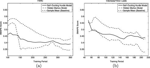
Figure 9: SMAPE scores for the three models with (a) FARC data and (b) Indonesia/Timor-Leste data.

We now provide a qualitative comparison between the TAR, SEHM and HMM frameworks. While all the three models assume that the current observation/activity is dependent on the past history, the models differ in how this dependence is realized. In particular, in the TAR model, the current observation is explicitly dependent on the past observations along with (possibly) the impact from other independent variables corresponding to certain geopolitical events/interventions. On the other hand, in the SEHM, the probability of an attack is enhanced by the history of the group according to the formula:

$$\frac{\mathsf{P}(M_{i}>0|{\mathcal{H}}_{i-1})|_{\mathsf{SEHM}}}{\mathsf{P}(M_{i}>0|{\mathcal{H}}_{i-1})|_{\mathsf{Non\mbox{-}SEHM}}}=1+\frac{e^{-B_{i}}}{1-e^{-B_{i}}}\cdot\bigl{(}1-e^{-\operatorname{SE}_{i}({\mathcal{H}}_{i-1})}\bigr{)}\geq 1.$$

The HMM combines both these facets by introducing a hidden state sequence. The state sequence depends explicitly on its most immediate past (one-step Markovian structure), whereas the probability of an attack is enhanced based on the state realization.

The TAR model and the HMM are similar from the viewpoint of regime switching, as these features are modeled explicitly. However, the mechanism of regime switching is different in the two cases: the former assumes a change in the auto-regressive process, whereas the latter assumes a state transition in the HMM. The SEHM also incorporates a switch between states (induced by the self-exciting component), but this switch is more of an implicit feature of the model rather than an explicit component.

More importantly, the TAR model considers global terrorism trends rather than trends constrained to a specific region or a specific group. Similarly, the Indonesia/Timor-Leste data set considered by Porter and White (2012) is a collation of all attacks in Indonesia and Timor-Leste from diverse groups with significantly different Intentions and Capabilities profiles such as Dar-ul-Islam, Gerakan Aceh Merdeka, Jemaah Islamiyah, etc. On the other hand, the FARC data set considered here is exclusively the action of the many sub-groups of FARC. This distinction between activity across groups in a specific region versus group-based activity could explain why the HMM leads to a better model fit for the FARC data set relative to the SEHM. This logic also suggests that the HMM may be a poorer model for regional/global trends. This hypothesis deserves a more careful study and is the subject of current work.

7 Concluding remarks

This work develops a HMM framework to model the activity profile of terrorist groups. Key to this development is the hypothesis that the current activity of the group can be captured completely by certain states/attributes of the group, instead of the entire past history of the group. In the simplest example of the proposed framework, the group’s activity is captured by a $d=2$ state HMM with the states reflecting a low state of activity (Inactive) and a high state of activity (Active), respectively. In either state, the days of activity are modeled as a discrete-time Poisson point process with a hurdle-based geometric model being a good fit for the number of attacks per day. While more general models can be considered, even the simplest framework is sufficient for detecting spurts and downfalls in the activity profile of many groups of interest. Our results show that the HMM approach provides a competent alternate modeling framework to the TAR and SEHM approaches, both in terms of explanatory and predictive powers.

Fruitful directions to explore in the future include development of more refined models for the activity profile (such as hierarchical HMMs) that incorporate heavy tails and extreme outliers commonly observed in terrorism data. A systematic comparison between the TAR model, SEHM and HMM and a possible bridge between these classes will also be of interest. In terms of inferencing, nonlinear filtering approaches such as particle filters are of importance in practice. Given the intensive nature of data collection that is common for studies of this nature, it would be of interest in developing broad trends and trade-offs in quantitative terrorism studies with a large set of groups from different ideological proclivities.

[id=suppA] Supplement A Information on models for the number of attacks per day studied in this work [doi]10.1214/13-AOAS682SUPPA .pdf aoas682_suppa.pdf This section derives the ML and Baum–Welch estimate of model parameter(s) under the geometric and hurdle-based geometric assumptions on $\{M_{i}\}$.

[id=suppA] Supplement B Background information on FARC and shining path [doi]10.1214/13-AOAS682SUPPB .pdf aoas682_suppb.pdf This section motivates the choice of the terrorist groups and the corresponding time periods of interest that are the focus of this work.

References

- Baddeley, Møller and Waagepetersen (2000) {barticle}[mr] \bauthor\bsnmBaddeley, \bfnmA. J.\binitsA. J., \bauthor\bsnmMøller, \bfnmJ.\binitsJ. and \bauthor\bsnmWaagepetersen, \bfnmR.\binitsR. (\byear2000). \btitleNon- and semi-parametric estimation of interaction in inhomogeneous point patterns. \bjournalStat. Neerl. \bvolume54 \bpages329–350. \biddoi=10.1111/1467-9574.00144, issn=0039-0402, mr=1804002 \bptokimsref \endbibitem
- Cho et al. (2013) {bmisc}[author] \bauthor\bsnmCho, \bfnmY. S.\binitsY. S., \bauthor\bsnmGalstyan, \bfnmA.\binitsA., \bauthor\bsnmBrantingham, \bfnmP. J.\binitsP. J. and \bauthor\bsnmTita, \bfnmG.\binitsG. (\byear2013). \bhowpublishedLatent point process models for spatial-temporal networks. Available at \arxivurlarXiv:1302.2671. \bptokimsref \endbibitem
- Clauset and Gleditsch (2012) {barticle}[pbm] \bauthor\bsnmClauset, \bfnmAaron\binitsA. and \bauthor\bsnmGleditsch, \bfnmKristian Skrede\binitsK. S. (\byear2012). \btitleThe developmental dynamics of terrorist organizations. \bjournalPLoS ONE \bvolume7 \bpagese48633. \biddoi=10.1371/journal.pone.0048633, issn=1932-6203, pii=PONE-D-12-25296, pmcid=3504060, pmid=23185267 \bptokimsref \endbibitem
- Clauset, Young and Gleditsch (2007) {barticle}[author] \bauthor\bsnmClauset, \bfnmA.\binitsA., \bauthor\bsnmYoung, \bfnmM.\binitsM. and \bauthor\bsnmGleditsch, \bfnmK. S.\binitsK. S. (\byear2007). \btitleOn the frequency of severe terrorist events. \bjournalJournal of Conflict Resolution \bvolume51 \bpages58–87. \bptokimsref \endbibitem
- Cox and Isham (1980) {bbook}[mr] \bauthor\bsnmCox, \bfnmDavid Roxbee\binitsD. R. and \bauthor\bsnmIsham, \bfnmValerie\binitsV. (\byear1980). \btitlePoint Processes. \bpublisherChapman & Hall, \blocationLondon. \bidmr=0598033 \bptokimsref \endbibitem
- Cragin and Daly (2004) {bbook}[author] \bauthor\bsnmCragin, \bfnmK.\binitsK. and \bauthor\bsnmDaly, \bfnmS. A.\binitsS. A. (\byear2004). \btitleThe Dynamic Terrorist Threat: An Assessment of Group Motivations and Capabilities in a Changing World. \bpublisherRAND Corporation, \blocationSanta Monica, CA. \bptokimsref \endbibitem
- Cressie (1991) {bbook}[mr] \bauthor\bsnmCressie, \bfnmNoel A. C.\binitsN. A. C. (\byear1991). \btitleStatistics for Spatial Data. \bpublisherWiley, \blocationNew York. \bidmr=1127423 \bptokimsref \endbibitem
- Diggle (2003) {bbook}[author] \bauthor\bsnmDiggle, \bfnmP. J.\binitsP. J. (\byear2003). \btitleStatistical Analysis of Spatial Point Patterns, \bedition2nd ed. \bpublisherEdward Arnold, \blocationLondon. \bptokimsref \endbibitem
- Dixon (2002) {bincollection}[author] \bauthor\bsnmDixon, \bfnmP. M.\binitsP. M. (\byear2002). \btitleRipley’s function. In \bbooktitleEncyclopedia of Environmetrics (\beditor\bfnmA. H.\binitsA. H. \bsnmEl-Shaarawi and \beditor\bfnmW. W.\binitsW. W. \bsnmPiegorsc, eds.) \bvolume2 \bpages1796–1803. \bpublisherWiley, \blocationChichester. \bptokimsref \endbibitem
- Dugan, LaFree and Piquero (2005) {barticle}[author] \bauthor\bsnmDugan, \bfnmL.\binitsL., \bauthor\bsnmLaFree, \bfnmG.\binitsG. and \bauthor\bsnmPiquero, \bfnmA.\binitsA. (\byear2005). \btitleTesting a rational choice model of airline hijackings. \bjournalCriminology \bvolume43 \bpages1031–1066. \bptokimsref \endbibitem
- Durbin (1973) {bbook}[mr] \bauthor\bsnmDurbin, \bfnmJ.\binitsJ. (\byear1973). \btitleDistribution Theory for Tests Based on the Sample Distribution Function. \bpublisherSIAM, \blocationPhiladelphia, PA. \bidmr=0305507 \bptokimsref \endbibitem
- Enders and Sandler (1993) {barticle}[author] \bauthor\bsnmEnders, \bfnmW.\binitsW. and \bauthor\bsnmSandler, \bfnmT.\binitsT. (\byear1993). \btitleThe effectiveness of antiterrorism policies: A vector autoregression-intervention analysis. \bjournalThe American Political Science Review \bvolume87 \bpages829–844. \bptokimsref \endbibitem
- Enders and Sandler (2000) {barticle}[author] \bauthor\bsnmEnders, \bfnmW.\binitsW. and \bauthor\bsnmSandler, \bfnmT.\binitsT. (\byear2000). \btitleIs transnational terrorism becoming more threatening? A time-series investigation. \bjournalJournal of Conflict Resolution \bvolume44 \bpages307–332. \bptokimsref \endbibitem
- Enders and Sandler (2002) {barticle}[author] \bauthor\bsnmEnders, \bfnmW.\binitsW. and \bauthor\bsnmSandler, \bfnmT.\binitsT. (\byear2002). \btitlePatterns of transnational terrorism, 1970–1999: Alternative time-series estimates. \bjournalInternational Studies Quarterly \bvolume2 \bpages145–165. \bptokimsref \endbibitem
- Haugaard, Isacson and Olson (2005) {bmisc}[author] \bauthor\bsnmHaugaard, \bfnmL.\binitsL., \bauthor\bsnmIsacson, \bfnmA.\binitsA. and \bauthor\bsnmOlson, \bfnmJ.\binitsJ. (\byear2005). \bhowpublishedErasing the lines: Trends in U.S. military programs with Latin America. Technical report, Center for International Policy, Washington, DC. \bptokimsref \endbibitem
- Hawkes (1971) {barticle}[mr] \bauthor\bsnmHawkes, \bfnmAlan G.\binitsA. G. (\byear1971). \btitleSpectra of some self-exciting and mutually exciting point processes. \bjournalBiometrika \bvolume58 \bpages83–90. \bidissn=0006-3444, mr=0278410 \bptokimsref \endbibitem
- ITERATE (2004) {bmisc}[author] \borganizationITERATE (\byear2004). \bhowpublishedInternational terrorism: Attributes of terrorist events. Available at http://www.icpsr.umich.edu/icpsrweb/ICPSR/studies/07947. \bptokimsref \endbibitem
- LaFree and Dugan (2007) {barticle}[author] \bauthor\bsnmLaFree, \bfnmG.\binitsG. and \bauthor\bsnmDugan, \bfnmL.\binitsL. (\byear2007). \btitleIntroducing the global terrorism database. \bjournalTerrorism and Political Violence \bvolume19 \bpages181–204. \bptokimsref \endbibitem
- LaFree, Morris and Dugan (2010) {barticle}[author] \bauthor\bsnmLaFree, \bfnmG.\binitsG., \bauthor\bsnmMorris, \bfnmN. A.\binitsN. A. and \bauthor\bsnmDugan, \bfnmL.\binitsL. (\byear2010). \btitleCross-national patterns of terrorism, comparing trajectories for total, attributed and fatal attacks, 1970–2006. \bjournalBritish Journal of Criminology \bvolume50 \bpages622–649. \bptokimsref \endbibitem
- Lewis et al. (2011) {barticle}[author] \bauthor\bsnmLewis, \bfnmE.\binitsE., \bauthor\bsnmMohler, \bfnmG. O.\binitsG. O., \bauthor\bsnmBrantingham, \bfnmP. J.\binitsP. J. and \bauthor\bsnmBertozzi, \bfnmA.\binitsA. (\byear2011). \btitleSelf-exciting point process models of civilian deaths in Iraq. \bjournalSecurity Journal \bvolume25 \bpages244–264. \bptokimsref \endbibitem
- Lindberg (2010) {bmisc}[author] \bauthor\bsnmLindberg, \bfnmM.\binitsM. (\byear2010). \bhowpublishedFactors contributing to the strength and resilience of terrorist groups. Grupo de Estudios Estrategicos (GEES) Publication. \bptokimsref \endbibitem
- Midlarsky (1978) {barticle}[author] \bauthor\bsnmMidlarsky, \bfnmM. I.\binitsM. I. (\byear1978). \btitleAnalyzing diffusion and contagion effects: The urban disorders of the 1960s. \bjournalThe American Political Science Review \bvolume72 \bpages996–1008. \bptokimsref \endbibitem
- Midlarsky, Crenshaw and Yoshida (1980) {barticle}[author] \bauthor\bsnmMidlarsky, \bfnmM. I.\binitsM. I., \bauthor\bsnmCrenshaw, \bfnmM.\binitsM. and \bauthor\bsnmYoshida, \bfnmF.\binitsF. (\byear1980). \btitleWhy violence spreads: The contagion of international terrorism. \bjournalInternational Studies Quarterly \bvolume24 \bpages262–298. \bptokimsref \endbibitem
- Mohler et al. (2011) {barticle}[mr] \bauthor\bsnmMohler, \bfnmG. O.\binitsG. O., \bauthor\bsnmShort, \bfnmM. B.\binitsM. B., \bauthor\bsnmBrantingham, \bfnmP. J.\binitsP. J., \bauthor\bsnmSchoenberg, \bfnmF. P.\binitsF. P. and \bauthor\bsnmTita, \bfnmG. E.\binitsG. E. (\byear2011). \btitleSelf-exciting point process modeling of crime. \bjournalJ. Amer. Statist. Assoc. \bvolume106 \bpages100–108. \biddoi=10.1198/jasa.2011.ap09546, issn=0162-1459, mr=2816705 \bptokimsref \endbibitem
- Mueller and Stewart (2011) {bbook}[author] \bauthor\bsnmMueller, \bfnmJ.\binitsJ. and \bauthor\bsnmStewart, \bfnmM. G.\binitsM. G. (\byear2011). \btitleTerrorism, Security, and Money: Balancing the Risks, Benefits, and Costs of Homeland Security. \bpublisherOxford Univ. Press, \blocationLondon. \bptokimsref \endbibitem
- Ogata (1988) {barticle}[author] \bauthor\bsnmOgata, \bfnmY.\binitsY. (\byear1988). \btitleStatistical models for earthquake occurrences and residual analysis for point processes. \bjournalJ. Amer. Statist. Assoc. \bvolume83 \bpages9–27. \bptokimsref \endbibitem
- Ogata (1998) {barticle}[author] \bauthor\bsnmOgata, \bfnmY.\binitsY. (\byear1998). \btitleSpace–time point process models for earthquake occurrences. \bjournalAnn. Inst. Statist. Math. \bvolume50 \bpages379–402. \bptokimsref \endbibitem
- Porter and White (2012) {barticle}[mr] \bauthor\bsnmPorter, \bfnmMichael D.\binitsM. D. and \bauthor\bsnmWhite, \bfnmGentry\binitsG. (\byear2012). \btitleSelf-exciting hurdle models for terrorist activity. \bjournalAnn. Appl. Stat. \bvolume6 \bpages106–124. \biddoi=10.1214/11-AOAS513, issn=1932-6157, mr=2951531 \bptokimsref \endbibitem
- Rabiner (1989) {barticle}[author] \bauthor\bsnmRabiner, \bfnmL. R.\binitsL. R. (\byear1989). \btitleA tutorial on hidden Markov models and selected applications in speech recognition. \bjournalProceedings of the IEEE \bvolume77 \bpages257–286. \bptokimsref \endbibitem
- Raghavan, Galstyan and Tartakovsky (2012) {bmisc}[author] \bauthor\bsnmRaghavan, \bfnmV.\binitsV., \bauthor\bsnmGalstyan, \bfnmA.\binitsA. and \bauthor\bsnmTartakovsky, \bfnmA. G.\binitsA. G. (\byear2012). \bhowpublishedHidden Markov models for the activity profile of terrorist groups. Available at \arxivurlarXiv:1207.1497v2. \bptokimsref \endbibitem
- Raghavan, Galstyan and Tartakovsky (2013a) {bmisc}[author] \bauthor\bsnmRaghavan, \bfnmV.\binitsV., \bauthor\bsnmGalstyan, \bfnmA.\binitsA. and \bauthor\bsnmTartakovsky, \bfnmA. G.\binitsA. G. (\byear2013a). \bhowpublishedSupplement to “Hidden Markov models for the activity profile of terrorist groups.” DOI:\doiurl10.1214/13-AOAS682SUPPA. \bptokimsref \endbibitem
- Raghavan, Galstyan and Tartakovsky (2013b) {bmisc}[author] \bauthor\bsnmRaghavan, \bfnmV.\binitsV., \bauthor\bsnmGalstyan, \bfnmA.\binitsA. and \bauthor\bsnmTartakovsky, \bfnmA. G.\binitsA. G. (\byear2013b). \bhowpublishedSupplement to “Hidden Markov models for the activity profile of terrorist groups.” DOI:\doiurl10.1214/13-AOAS682SUPPB. \bptokimsref \endbibitem
- (33) {bmisc}[author] \borganizationRDWTI. \bhowpublishedRAND database of worldwide terrorism incidents. Available at http://www.rand.org/nsrd/projects/terrorism-incidents.html. \bptokimsref \endbibitem
- Santos (2011) {barticle}[author] \bauthor\bsnmSantos, \bfnmD. N.\binitsD. N. (\byear2011). \btitleWhat constitutes terrorist network resiliency? \bjournalSmall Wars Journal \bvolume7. \bptokimsref \endbibitem
- Seshadri, Csorgo and Stephens (1969) {barticle}[author] \bauthor\bsnmSeshadri, \bfnmV.\binitsV., \bauthor\bsnmCsorgo, \bfnmM.\binitsM. and \bauthor\bsnmStephens, \bfnmM. A.\binitsM. A. (\byear1969). \btitleTests for the exponential distribution using Kolmogorov-type statistics. \bjournalJ. R. Stat. Soc. Ser. B Stat. Methodol. \bvolume31 \bpages499–509. \bptokimsref \endbibitem
- Teerapabolarn (2012) {barticle}[mr] \bauthor\bsnmTeerapabolarn, \bfnmK.\binitsK. (\byear2012). \btitleA pointwise approximation of generalized binomial by Poisson distribution. \bjournalAppl. Math. Sci. (Ruse) \bvolume6 \bpages1095–1104. \bidissn=1312-885X, mr=2902094 \bptokimsref \endbibitem
- Veen and Schoenberg (2006) {bincollection}[author] \bauthor\bsnmVeen, \bfnmA.\binitsA. and \bauthor\bsnmSchoenberg, \bfnmF. P.\binitsF. P. (\byear2006). \btitleAssessing spatial point process models using weighted -functions. In \bbooktitleCase Studies in Spatial Point Process Modeling (\beditor\binitsA.\bfnmA. \bsnmBaddeley \betalet al., eds.). \bseriesLecture Notes in Statistics \bvolume185 \bpages293–306. \bpublisherSpringer, \blocationNew York. \bptokimsref \endbibitem