From scattering theory to complex wave dynamics in non-hermitian $\mathcal{PT}$-symmetric resonators

Abstract

I review how methods from mesoscopic physics can be applied to describe the multiple wave scattering and complex wave dynamics in non-hermitian $\mathcal{PT}$-symmetric resonators, where an absorbing region is coupled symmetrically to an amplifying region. Scattering theory serves as a convenient tool to classify the symmetries beyond the single-channel case and leads to effective descriptions which can be formulated in the energy domain (via Hamiltonians) and in the time domain (via time evolution operators). These models can then be used to identify the mesoscopic time and energy scales which govern the spectral transition from real to complex eigenvalues. The possible presence of magneto-optical effects (a finite vector potential) in multichannel systems leads to a variant (termed $\mathcal{PTT}^{\prime}$ symmetry) which imposes the same spectral constraints as $\mathcal{PT}$ symmetry. I also provide multichannel versions of generalized flux-conservation laws.

I Introduction and Motivation

Optical systems combining lossy and active elements provide a platform to implement analogues of non-hermitian $\mathcal{PT}$-symmetric quantum systems bender ; ptreview1 ; ptreview2 , which allows to realize unique optical switching effects christodoulidesgroup1 ; christodoulidesgroup2 ; christodoulidesgroup3 ; ptexperiments1 ; ptexperiments2 ; pteffects1 ; pteffects2a ; pteffects4 ; pteffects5 ; hsqoptics ; longhilaserabsorber ; variousstonepapers1 ; variousstonepapers2 ; yoo ; schomerusyh . The wave scattering and dynamics in these systems provide an aspect which also permeates mesoscopic phenomena in microcavity lasers vahala , coherent electronic transport beenakkerreview ; datta , superconductivity beenakkerreview ; altlandzirnbauer , and quantum-chaotic dynamics haake . The main goal here is to relate how tools established in these disciplines can be used to approach the exciting spectral and dynamical features in $\mathcal{PT}$-symmetric optics. Scattering theory beenakkerreview ; datta ; fyodorovsommers , in particular, is ideally suited to deal with the complications of complex wave dynamics in multichannel situations, which appear when one goes beyond one-dimensional situations, and also easily accounts for any leakage if a system is geometrically open, as is often required by the nature of the desired optical effects, or because of the design of practical devices.

We thus describe in detail how this approach can be applied to optical realizations of $\mathcal{PT}$-symmetric systems with a wide range of geometries hsqoptics ; longhilaserabsorber ; variousstonepapers1 ; variousstonepapers2 ; yoo ; hsrmt ; birchallweyl ; birchallrmt . (For $\mathcal{PT}$-symmetric scattering in effectively one dimension see, e.g., Refs. cannata ; berry ; jones .) To formulate the approach under these conditions it matters whether a geometric symmetry inverts or preserves the handedness of the coordinate system, especially in the presence of magneto-optical effects (vector potentials, which generally cannot be gauged away beyond one dimension). An analogous bifurcation arises in the specification of the time-reversal operation. Moreover, it is important to note that the fields defining a device geometry are external, a distinction from particle-physics settings which is reflected in the subtleties of Onsager’s reciprocal relations onsager . Thus the formulation of $\mathcal{PT}$ symmetry itself requires some care. In particular, an alternative appears, termed $\mathcal{PTT}^{\prime}$ symmetry hsrmt , which results in the same spectral constraints but imposes different physical symmetry conditions. The scattering approach also allows to restate the symmetry requirements in terms of generalized conservation laws variousstonepapers2 , which we here extend to multiple channels. Furthermore, the approach leads to effective models of complex wave dynamics which relate the spectral features to universal mesoscopic time and energy scales hsrmt ; birchallweyl ; birchallrmt .

We start this exposition with a brief recapitulation of the analogy between optics and non-hermitian quantum mechanics (section II), and discuss variants of geometric and time-reversal operations which can be used to set up $\mathcal{PT}$ and $\mathcal{PTT}^{\prime}$ symmetry (section III and section IV). We then describe how scattering theory can be applied to study the spectral features in these settings, first generally (section V-section VII) and then for a coupled-resonator geometry (section VIII). This leads to effective models (section IX) which can be formulated in the energy domain (via Hamiltonians) and in the time domain (via time evolution operators), and capture the relevant energy and time scales (section X). The concluding section XI also describes possible generalizations of these models.

II Optical analogues of non-hermitian quantum mechanics

The $\mathcal{PT}$-symmetric optical systems mentioned in the introduction cover a large range of designs, including coupled optical fibres, photonic crystals and coupled resonators, as depicted in figure 1. Some of the elements are absorbing while others are amplifying, and the absorption and amplification rates, geometry, and other material properties are carefully matched to result in a symmetric arrangement.

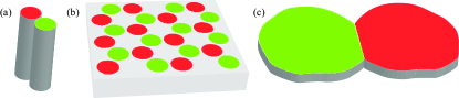
Figure 1: (Online version in colour.) Common designs of $\mathcal{PT}$-symmetric optical systems with absorbing (light green) and amplifying (dark red) elements. (a) Two optical fibers. (b) Localized modes in a photonic crystals. (c) Coupled-resonator geometry.

We concentrate on two common designs, effectively two-dimensional systems (planar resonators or photonic crystals, with coordinates $x$, $y$) as well as three-dimensional pillar-like systems (such as arrangements of aligned optical fibers with a fixed cross section) where the geometry does not depend on the third coordinate $z$, and assume that the relevant effects of wave scattering, gain and loss can be subsumed in a refractive index $n(\mathbf{r})$, where ${\rm Im}\,n(\mathbf{r})>0$ signifies absorption (loss) while ${\rm Im}\,n(\mathbf{r})<0$ signifies amplification (gain). Later on, we also include an external vector potential $\mathbf{A}(\mathbf{r})$ representing magneto-optical effects.

These assumptions allow to separate transverse magnetic (TM) and electric (TE) modes, with the magnetic or electric field, respectively, confined to the $xy$-plane (thus transverse to $z$). The electromagnetic field can then be described by a scalar wave function $\psi({\bf r})$, which represents the $z$-component of the electric or magnetic field, respectively. One now arrives at two principal situations, which both serve as an optical analogue of non-hermitian quantum mechanics.

II.1 Helmholtz equation

On the one hand, one can focus on the propagation in the $xy$-plane, resulting in an effectively two-dimensional system which is described by a Helmholtz equation

$$\mathcal{L}(\omega)\psi({\bf r})=0,$$

$$\mathcal{L}(\omega)=\left\{\begin{array}[]{cc}\nabla^{2}+\frac{\omega^{2}n^{2}({\bf r})}{c^{2}}&\mbox{(TM)}\\ \nabla\frac{1}{n^{2}({\bf r})}\nabla+\frac{\omega^{2}}{c^{2}}&\mbox{(TE)}\end{array}\right.,\quad\nabla=\left(\begin{array}[]{c}\partial_{x}\\ \partial_{y}\end{array}\right).$$ (5)

The Helmholtz equation is analogous to a stationary Schrödinger equation, thus, an eigenvalue problem for the frequencies $\omega$, which can become complex due to the loss and gain encoded in $n$, or because of leakage at the boundaries of the system in the propagation plane. This then describes quasistationary states which decay (${\rm Im}\,\omega<0$) or grow (${\rm Im}\,\omega>0$) over time.

II.2 Paraxial equation

On the other hand, one can focus on the propagation into the $z$-direction perpendicular to this plane, which is then often described by a paraxial equation

$$2i\kappa\partial_{z}\psi({\bf r})+\mathcal{L}(\kappa)\psi({\bf r})=0,$$

$${\mathcal{L}}(\kappa)=\left\{\begin{array}[]{cc}\nabla^{2}+\frac{\omega^{2}n^{2}({\bf r})}{c^{2}}-\kappa^{2}&\mbox{(TM)}\\ n^{2}({\bf r})\nabla\frac{1}{n^{2}({\bf r})}\nabla+\frac{\omega^{2}n^{2}({\bf r})}{c^{2}}-\kappa^{2}&\mbox{(TE)}\end{array}\right..$$ (8)

Here $\psi({\bf r})$ now is an envelope wave function, obtained after separating out a term $\exp(i\kappa z)$. This equation remains valid if $n$ varies only slowly with $z$, $|\partial_{z}n/n|\ll|\kappa|$.

The paraxial equation is an analogue of a time-dependent Schrödinger equation, thus, a dynamical equation where an initial condition is propagated forwards—here, not in time, but along the spatial direction with coordinate $z$. It is then natural to probe the system at an initial and a final cross-section, while the physical frequency $\omega$ is now real.

As we assume that $n$ is $z$-independent, the paraxial equation is associated with the eigenvalue problem $\mathcal{L}(\kappa)\psi({\bf r})=0$ for the propagation constant $\kappa$. This eigenvalue problem shares all relevant mathematical features with the problem (II.1) for $\omega$ (in particular, the eigenvalues again can be complex because of loss, gain, and leakage in the system); so do variants that rely on wave localization in the cores of optical fibers or Wannier-like modes in a photonic crystal, with the gradient replaced by hopping terms. For definiteness, we shall employ notations adapted to the eigenvalue problem for $\omega$.

III Symmetries of the wave equation

The investigation of symmetries in higher-dimensional systems of arbitrary geometry is a central aspect of mesoscopic physics. For hermitian systems, a complete classification requires to take care of magnetic fields, internal degrees of freedom such as spin, pairing potentials and particle-hole symmetries beenakkerreview ; datta ; altlandzirnbauer ; haake . Non-hermitian systems provide an even wider setting, with a mathematical classification, e.g., provided in Ref. magnea . In order to identify and specify the role of symmetries for their optical realizations we denote the operator in the wave equation by $\mathcal{L}(\omega;n(\mathbf{r}))$, which explicitly takes care of the functional dependence on the refractive index $n$.

III.1 $\mathcal{PT}$ symmetry

In $\mathcal{PT}$-symmetric quantum mechanics bender ; ptreview1 ; ptreview2 , the parity operator $\mathcal{P}$ generally stands for a unitary transformation which squares to the identity. In optical systems, this operation is usually realized geometrically via an isometric involution, still denoted as $\mathcal{P}$, which inverts one, two, or three coordinates. To specify the consequences for the wave equation we promote ${\cal P}$ to a superoperator (we employ this notation as we will also encounter a transformation $\mathcal{T}^{\prime}$ which does not correspond to an ordinary unitary or antiunitary operator). Then

$$\mathcal{P}[\mathcal{L}(\omega;n(\mathbf{r}))]=\mathcal{L}(\omega;n(\mathcal{P}\mathbf{r})),$$ (9)

which should be read as a rule how to write the wave equation in the transformed coordinate system. The transformed equation is then solved by ${\cal P}\psi({\bf r})\equiv\psi({\cal P}{\bf r})$.

Conventional time reversal is implemented by complex conjugation in the position representation, which constitutes an antiunitary operation. We then have

$$\mathcal{T}[\mathcal{L}(\omega;n(\mathbf{r}))]=\mathcal{L}(\omega^{*};n^{*}(\mathbf{r})),$$ (10)

which delivers a wave equation solved by ${\cal T}\psi({\bf r})\equiv\psi^{*}({\bf r})$.

The wave equation now displays $\mathcal{PT}$ symmetry if the refractive index obeys $n({\bf r})=n^{*}({\cal P}{\bf r})$. In this situation ${\cal P}$ is an involution that interchanges amplifying and absorbing regions with matching amplification and absorption rates, and

$$\mathcal{PT}[\mathcal{L}(\omega;n(\mathbf{r}))]=\mathcal{L}(\omega^{*};n^{*}(\mathcal{P}\mathbf{r}))=\mathcal{L}(\omega^{*};n(\mathbf{r})),$$ (11)

which constraints the spectral properties of $\mathcal{L}$ if the boundary conditions also respect the symmetry (this is typically not the case if the system is open). The eigenvalues $\omega_{n}$ then obey

$$\omega_{n}=\omega^{*}_{\bar{n}}$$ (12)

and thus either real ($n=\bar{n}$) if $\psi^{*}_{n}(\mathcal{P}\mathbf{r})$ linearly depends on $\psi_{n}(\mathbf{r})$, or occur in complex-conjugate pairs ($n\neq\bar{n}$) if that is not the case.

III.2 $\mathcal{T^{\prime}}$ symmetry

It is important to distinguish the conventional antiunitary time-reversal operation ${\cal T}$ from another operation that is also often termed time-reversal beenakkerreview ; datta ; altlandzirnbauer ; haake . If $\mathcal{L}({\bf r})$ were hermitian ($\omega$ and $n$ both real with appropriate boundary conditions), then the action of ${\cal T}$ could not be distinguished from the action of a superoperator ${\cal T}^{\prime}$ acting in the position representation as

$${\cal T}^{\prime}[\mathcal{L}(\omega;n(\mathbf{r}))]=\mathcal{L}^{T}(\omega;n(\mathbf{r})).$$ (13)

Thus, ${\cal T}^{\prime}$ transforms the right eigenvalue problem ${\cal L}\psi=0$ into the left eigenvalue problem ${\cal L}^{T}\bar{\psi}=0$. This delivers the same spectrum, and while the right and left eigenfunctions $\psi$ and $\bar{\psi}$ for a given eigenvalue generally differ they are related by biorthogonality constraints. In the presently assumed absence of magneto-optical effects, ${\cal T}^{\prime}$ is indeed an exact symmetry, $\mathcal{L}^{T}(\omega;n(\mathbf{r}))=\mathcal{L}(\omega;n(\mathbf{r}))$ and thus $\psi=\bar{\psi}$. This holds even if $n$ is complex, thus, even if ${\cal T}$ symmetry is broken. In the non-hermitian case, therefore, these two operations are distinct and must be treated separately.

IV Magneto-optical effects

In mesoscopic systems with complex wave dynamics, the alternative time-reversal operation ${\cal T}^{\prime}$ governs a multitude of effects ranging from coherent backscattering and wave localization to minigaps in mesoscopic superconductors beenakkerreview ; datta ; altlandzirnbauer ; melsen . To clarify the role of this operation we now consider magneto-optical effects, which are described by a (possibly complex) external vector potential $\mathbf{A}(\mathbf{r})$ that enters the wave equation through terms of the generic form $(\nabla+i\mathbf{A}(\mathbf{r}))^{2}$. For this purpose we denote the operator in the wave equation as $\mathcal{L}(\omega;n(\mathbf{r}),\mathbf{A}(\mathbf{r}))$. As before, we continue to focus on effectively two-dimensional systems; thus, $A_{z}=0$, see (II.1) and (8).

IV.1 $\mathcal{PT}$ symmetry

The involution $\mathcal{P}$ (interpreted as a coordinate transformation of the wave equation) transforms the external vector potential according to $(\nabla+i\mathbf{A}(\mathbf{r}))^{2}\to({\cal P}\nabla+i\mathbf{A}({\cal P}\mathbf{r}))^{2}=(\nabla+i[{\cal P}\mathbf{A}]({\cal P}\mathbf{r}))^{2}$, as ${\cal P}$ is an isometry. Thus

$$\mathcal{P}[\mathcal{L}(\omega;n(\mathbf{r}),\mathbf{A}(\mathbf{r}))]=\mathcal{L}(\omega;n(\mathcal{P}\mathbf{r}),[\mathcal{P}\mathbf{A}](\mathcal{P}\mathbf{r})).$$ (14)

This analysis reveals an important feature of parity when applied to external fields, which sets them apart from internal fields that are often discussed in the setting of particle physics, and then are subject to additional explicit transformation rules. Here we are interested in symmetries of a wave function $\psi({\bf r})$ that only accounts for the internal system dynamics, not for external components such as the motion of electrons in the inductors or the magnetic moments in the permanent magnets generating the field. This distinction is fundamental for Onsager’s reciprocal relations, which break down in the presence of external magnetic fields onsager . The resulting magnetic field depends on whether $\mathcal{P}$ preserves or inverts the handedness of the coordinate system, as $\nabla\times\mathcal{P}\mathbf{A}(\mathcal{P}\mathbf{r})={\rm det}(\mathcal{P})\mathcal{P}[\nabla\times\mathbf{A}(\mathbf{r})]$.

The time-reversal operator $\mathcal{T}$ transforms $(\nabla+i\mathbf{A}(\mathbf{r}))^{2}\to(\nabla-i\mathbf{A}^{*}(\mathbf{r}))^{2}$, so

$$\mathcal{T}[\mathcal{L}(\omega;n(\mathbf{r}),\mathbf{A}(\mathbf{r}))]=\mathcal{L}(\omega^{*};n^{*}(\mathbf{r}),-\mathbf{A}^{*}(\mathbf{r})).$$ (15)

$\mathcal{PT}$ symmetry thus requires

$$n({\bf r})=n^{*}({\cal P}{\bf r}),\quad\mathbf{A}({\bf r})=-\mathcal{P}\mathbf{A}^{*}({\cal P}{\bf r}).$$ (16)

E.g., when ${\cal P}$ is a reflection $x\to-x$ this holds for a homogeneous magnetic field that points in the $z$ direction [see figure 2(a)].

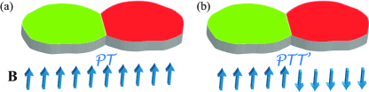
Figure 2: (Online version in colour.) Illustration of magneto-optical effects (associated with an effective magnetic field $\mathbf{B}$) for (a) $\mathcal{PT}$ symmetry and (b) $\mathcal{PTT}^{\prime}$ symmetry, where $\mathcal{P}$ is a reflection hsrmt .

IV.2 $\mathcal{PTT}^{\prime}$ symmetry

We now identify a modified symmetry, which eventually yields the same spectral constraints as obtained for $\mathcal{PT}$ symmetry, but imposes a different condition on the magnetic field hsrmt . This variant follows from the inspection of the $\mathcal{T^{\prime}}$ operation. In the position representation $\partial_{x}^{T}=-\partial_{x}$, $\partial_{y}^{T}=-\partial_{y}$ (recall that we focus on the effects in the 2D cross-sectional plane), and thus

$$\mathcal{T^{\prime}}:\quad(\nabla+i\mathbf{A}(\mathbf{r}))^{2}\to[(\nabla+i\mathbf{A}(\mathbf{r}))^{2}]^{T}=(\nabla-i\mathbf{A}(\mathbf{r}))^{2}.$$ (17)

This effectively inverts the vector potential,

$${\cal T}^{\prime}[\mathcal{L}(\omega;n(\mathbf{r}),\mathbf{A}(\mathbf{r}))]=\mathcal{L}(\omega;n(\mathbf{r}),-\mathbf{A}(\mathbf{r})),$$ (18)

which confirms that ${\cal T}^{\prime}$ symmetry is broken when $\mathbf{A}$ is finite. Consider now

$$\mathcal{PTT^{\prime}}[\mathcal{L}(\omega;n({\bf r}),\mathbf{A}({\bf r})]=\mathcal{L}(\omega^{*};n^{*}({\cal P}{\bf r}),\mathcal{P}\mathbf{A}^{*}({\cal P}{\bf r})).$$ (19)

This turns into a symmetry if

$$n({\bf r})=n^{*}({\cal P}{\bf r}),\quad\mathbf{A}({\bf r})=\mathcal{P}\mathbf{A}^{*}({\cal P}{\bf r}).$$ (20)

E.g., when ${\cal P}$ is a reflection $x\to-x$ this holds for an antisymmetric magnetic field which (in the plane of the resonator) points in the $z$ direction [see figure 2(b)].

V Scattering formalism

The optical systems considered here are naturally open, with leakage occurring, e.g., at the fiber tips and waveguide entries, or because the confinement in the cross-section relies on partial internal reflection at refractive index steps or semitransparent mirrors. These systems can thus be probed via scattering beenakkerreview ; datta ; fyodorovsommers , which delivers comprehensive insight into their spectral and dynamical properties and illuminates the consequences of the symmetries discussed above, as well as the role of multiple scattering addressed later on.

These properties are encoded in the scattering matrix $S(\omega)$, which relates the amplitudes $a_{\mathrm{in},n}$, $a_{\mathrm{out},n}$ in incoming and outgoing scattering states $\chi_{\mathrm{in},n}$, $\chi_{\mathrm{out},n}$,

$$\mathbf{a}_{\mathrm{out}}=S(\omega)\mathbf{a}_{\mathrm{in}}.$$ (21)

This relation is generally obtained by the solution of the wave equation under appropriate conditions at the boundary $\partial\Omega$ of the scattering region $\Omega$ (outside of which we set $n=1$, ${\bf A}=0$). The scattering states are assumed to be flux orthonormalised,

$$\int_{\partial\Omega}d\mathbf{S}\cdot[\chi_{\sigma,n}^{*}\nabla\chi_{\sigma^{\prime},m}-\chi_{\sigma^{\prime},m}\nabla\chi_{\sigma,n}^{*}]=2i\sigma\delta_{nm}\delta_{\sigma\sigma^{\prime}},$$ (22)

where $\sigma=1$ for outgoing states and $\sigma=-1$ for incoming states. Two popular choices are states with fixed angular momentum in free space, and transversely quantized modes in a fixed-width waveguide geometry.

We now describe the adaptation of this formalism to $\mathcal{PT}$ and $\mathcal{PTT}^{\prime}$-symmetric situations hsqoptics ; longhilaserabsorber ; variousstonepapers1 ; variousstonepapers2 ; yoo ; hsrmt ; birchallweyl .

V.1 ${\cal PT}$ symmetry

The symmetries of a scattering problem are exposed when one conveniently groups the scattering states. To inspect ${\cal P}$ we call half of the incoming states ‘incoming from the left’, and the other half ‘incoming from the right’. This does not need to be taken literally; all what matters is that the two groups are converted into each other by ${\cal P}$. The same can be done for the outgoing states. The scattering matrix then decomposes into blocks,

$$S=\left(\begin{array}[]{cc}r&t^{\prime}\\ t&r^{\prime}\\ \end{array}\right),$$ (23)

where $r$ describes reflection of left incoming states into left outgoing states, $r^{\prime}$ describes the analogous reflection on the right, while $t$ and $t^{\prime}$ describe transmission from the left to the right and vice versa. The parity $\mathcal{P}$ interchanges the amplitudes of the left and right states, which can be brought about by a $\sigma_{x}$ Pauli matrix,

$$\mathcal{P}[S]=\sigma_{x}S\sigma_{x}=\left(\begin{array}[]{cc}r^{\prime}&t\\ t^{\prime}&r\\ \end{array}\right).$$ (24)

For consideration of the $\mathcal{T}$ operation, we group incoming and outgoing states into time-reversed pairs. When $\mathcal{T}$ acts on a wave function the amplitudes become conjugated, while the frequency in the wave equation changes to $\omega^{*}$. Furthermore, incoming states are converted into outgoing states, so that the relation (21) must be inverted. Thus,

$$\mathcal{T}[S(\omega)]=\{S^{-1}(\omega^{*})\}^{*}.$$ (25)

In combination, we have hsqoptics ; variousstonepapers1 ; yoo

$$\mathcal{PT}[S(\omega)]=\sigma_{x}\{S^{-1}(\omega^{*})\}^{*}\sigma_{x}.$$ (26)

A system with $\mathcal{PT}$ symmetry is then characterized by the invariance

$$\sigma_{x}\{S^{-1}(\omega^{*})\}^{*}\sigma_{x}=S(\omega),$$ (27)

which results in the constraint $\sigma_{x}S^{*}(\omega^{*})\sigma_{x}S(\omega)=\openone$, or

$$t^{\prime*}(\omega^{*})r(\omega)+r^{*}(\omega^{*})t(\omega) =0,$$

$$r^{\prime*}(\omega^{*})t^{\prime}(\omega)+t^{*}(\omega^{*})r^{\prime}(\omega) =0,$$

$$r^{*}(\omega^{*})r^{\prime}(\omega)+t^{\prime*}(\omega^{*})t^{\prime}(\omega) =\openone,$$

$$r^{\prime*}(\omega^{*})r(\omega)+t^{*}(\omega^{*})t(\omega) =\openone.$$ (28)

V.2 ${\cal PTT}^{\prime}$ symmetry

In hermitian problems the scattering matrix is unitary if $\omega$ is real, and the ${\cal T}$ operation is equivalent to the operation beenakkerreview ; datta

$$\mathcal{T}^{\prime}[S(\omega)]=S^{T}(\omega),$$ (29)

which corresponds to the operation identified above by inspection of the wave equation. In non-hermitian settings, this delivers the solution of the scattering problem associated with the transposed wave equation $\mathcal{L}^{T}\bar{\psi}(\mathbf{r})=0$,

$$\bar{\mathbf{a}}_{\mathrm{out}}=S^{T}(\omega)\bar{\mathbf{a}}_{\mathrm{in}}.$$ (30)

In ordinary optics, where $\textbf{A}=0$, $\mathcal{T}^{\prime}$ remains an exact symmetry even when $n$ and $\omega$ are complex. We then find the important constraint $S(\omega)=S^{T}(\omega)$, thus

$$r=r^{T},\quad r^{\prime}=r^{\prime T},\quad t^{\prime}=t^{T}.$$ (31)

The combined operation

$$\mathcal{PTT}^{\prime}[S(\omega)]=\sigma_{x}\{S^{-1}(\omega^{*})\}^{\dagger}\sigma_{x}$$ (32)

turns into a symmetry if hsrmt

$$t^{\dagger}(\omega^{*})r(\omega)+r^{\dagger}(\omega^{*})t(\omega) =0,$$

$$r^{\prime\dagger}(\omega^{*})t^{\prime}(\omega)+t^{\prime\dagger}(\omega^{*})r^{\prime}(\omega) =0,$$

$$r^{\dagger}(\omega^{*})r^{\prime}(\omega)+t^{\dagger}(\omega^{*})t^{\prime}(\omega) =\openone,$$

$$r^{\prime\dagger}(\omega^{*})r(\omega)+t^{\prime\dagger}(\omega^{*})t(\omega) =\openone.$$ (33)

This is realized for systems obeying the symmetry requirements (16).

VI Generalized flux conservation

For hermitian systems ($\omega$, $n$ and $\mathbf{A}$ all real), the unitarity $S^{\dagger}S=\openone$ of the scattering matrix ensures the conservation of the probability flux, $\mathbf{a}_{\mathrm{in}}^{\dagger}\mathbf{a}_{\mathrm{in}}=\mathbf{a}_{\mathrm{out}}^{\dagger}\mathbf{a}_{\mathrm{out}}$. In Ref. variousstonepapers2 analogous conservation laws were established for one-dimensional non-hermitian systems with $\mathcal{PT}$ symmetry, and it was found that these laws are automatically guaranteed by the symmetry conditions (V.1). These flux conditions only apply at real $\omega$, but provide a useful alternative perspective on the role of symmetry. Here we extend these conditions to higher-dimensional (multichannel) systems, include magneto-optical effects, and also allow for $\mathcal{PTT}^{\prime}$ symmetry (these considerations are original).

To illustrate the general strategy we consider the Helmholtz equation for TM polarization, with ${\bf A}=0$ and $\omega$ real. Thus $\psi(\mathbf{r})$ and $\psi^{*}(\mathcal{P}\mathbf{r})$ both solve the same wave equation $\mathcal{L}(\omega)\psi(\mathbf{r})=\mathcal{L}(\omega)\psi^{*}(\mathcal{P}\mathbf{r})=0$, with $\mathcal{L}(\omega)$ specified in equation (II.1). Now take the following volume integral over the region $\Omega$,

$$0 =\int_{\Omega}d\mathbf{r}\,[\psi^{*}(\mathcal{P}\mathbf{r})\mathcal{L}(\omega)\psi(\mathbf{r})-\psi(\mathbf{r})\mathcal{L}(\omega)\psi^{*}(\mathcal{P}\mathbf{r})]$$

$$=\int_{\Omega}d\mathbf{r}\,[\psi^{*}(\mathcal{P}\mathbf{r})\nabla^{2}\psi(\mathbf{r})-\psi(\mathbf{r})\nabla^{2}\psi^{*}(\mathcal{P}\mathbf{r})]$$

$$=\int_{\Omega}d\mathbf{r}\,\nabla[\psi^{*}(\mathcal{P}\mathbf{r})\nabla\psi(\mathbf{r})-\psi(\mathbf{r})\nabla\psi^{*}(\mathcal{P}\mathbf{r})]$$

$$=\int_{\partial\Omega}d\mathbf{S}\cdot[\psi^{*}(\mathcal{P}\mathbf{r})\nabla\psi(\mathbf{r})-\psi(\mathbf{r})\nabla\psi^{*}(\mathcal{P}\mathbf{r})],$$ (34)

under application of Stoke’s theorem. The resulting surface integral can be evaluated with equation (22). This delivers the generalized flux-conservation law

$$\mathbf{a}_{\mathrm{in}}^{\dagger}\sigma_{x}\mathbf{a}_{\mathrm{in}}=\mathbf{a}_{\mathrm{out}}^{\dagger}\sigma_{x}\mathbf{a}_{\mathrm{out}}=\mathbf{a}_{\mathrm{in}}^{\dagger}S^{\dagger}(\omega)\sigma_{x}S(\omega)\mathbf{a}_{\mathrm{in}},$$ (35)

which together with $S(\omega)=S^{T}(\omega)$ (as $\mathbf{A}=0$) amounts to the constraints (V.1), specialized to the case where $\omega$ is real.

The same constraints follow for TE polarization (as $n=1$ outside $\Omega$, so that the refractive index does not feature in the surface integral). Next, we include a finite vector potential A. For $\mathcal{PTT}^{\prime}$ symmetry, one can follow the steps given above, which directly delivers the constraints (V.2) (again specialized to real $\omega$). The case of $\mathcal{PT}$ symmetry with finite vector potential is more intricate, as one then needs to invoke the transposed wave equation $\mathcal{L}^{T}(\omega)\bar{\psi}(\mathbf{r})=\mathcal{L}^{T}(\omega)\bar{\psi}^{*}(\mathcal{P}\mathbf{r})=0$. One then integrates

$$0 =\int_{\Omega}d\mathbf{r}\,[\bar{\psi}^{*}(\mathcal{P}\mathbf{r})\mathcal{L}(\omega)\psi(\mathbf{r})-\psi(\mathbf{r})\mathcal{L}^{T}(\omega)\bar{\psi}^{*}(\mathcal{P}\mathbf{r})]$$

$$=\int_{\partial\Omega}d\mathbf{S}\cdot[\bar{\psi}^{*}(\mathcal{P}\mathbf{r})\nabla\psi(\mathbf{r})-\psi(\mathbf{r})\nabla\bar{\psi}^{*}(\mathcal{P}\mathbf{r})],$$ (36)

which results in the generalized flux-conservation law $\bar{\mathbf{a}}_{\mathrm{in}}^{\dagger}\sigma_{x}\mathbf{a}_{\mathrm{in}}=\bar{\mathbf{a}}_{\mathrm{out}}^{\dagger}\sigma_{x}\mathbf{a}_{\mathrm{out}}$. In combination with equation (30), this condition now requires $\sigma_{x}=S^{*}(\omega)\sigma_{x}S(\omega)$, which is again automatically fulfilled if the scattering matrix obeys the symmetry constraints (V.1).

In all these cases, the generalized flux-conservation relations at real $\omega$ thus does not impose any extra conditions beyond the symmetry requirements of the scattering matrix.

VII Scattering quantization conditions

It is now interesting to ask how the spectral properties of $\mathcal{PT}$ or $\mathcal{PTT}^{\prime}$-symmetric systems emerge within the scattering approach. We contrast the case of open systems (where the symmetry operation relates quasibound states with perfectly absorbed states, thus, connects states of a different physical nature) with closed systems (where the symmetry operation relates ordinary bound states, thus, connects states of the same nature, whose spectral properties then are constrained).

VII.1 General quantization conditions for quasibound and perfectly absorbed states

Quasibound states fulfill the wave equation with purely outgoing boundary conditions, thus, $\mathbf{a}_{\mathrm{in}}=0$ but $\mathbf{a}_{\mathrm{out}}$ finite. In view of equation (21), this requires

$$||S(\omega)||=\infty,$$ (37)

and so $\omega$ has to coincide with a pole of the scattering matrix. This results in a quantization of the admitted frequencies $\omega_{n}$, which in general are complex.

Quasibound states describe systems which generate all radiation internally, and in particular, lasers hsqoptics ; longhilaserabsorber ; variousstonepapers1 ; variousstonepapers2 ; yoo . In a passive system the poles are confined to the lower half of the complex plane, with the decay enforced by the leakage. In an active system, however, gain may compensate the losses and result in a stationary state, which signifies lasing. The threshold is attained when the first pole reaches the real axis.

Recent works have turned the attention to perfectly absorbed states, for which the role of incoming and outgoing states is inverted longhilaserabsorber ; stonecpa1 . These boundary conditions translate to $||S(\omega)||=0$, which results in quantized frequencies $\widetilde{\omega}_{n}$ coinciding with the zeros of the scattering matrix.

For a passive system, where $\mathcal{TT}^{\prime}[\mathcal{L}(\omega)]=\mathcal{L}(\omega^{*})$, a quasibound state $\psi_{n}(\mathbf{r})$ can be converted into a perfectly absorbed state $\widetilde{\psi}_{n}(\mathbf{r})=\bar{\psi}_{n}^{*}(\mathbf{r})$ by the $\mathcal{TT}^{\prime}$ operation [for exact $\mathcal{T}^{\prime}$ symmetry one simply has $\widetilde{\psi}_{n}(\mathbf{r})=\psi_{n}^{*}(\mathbf{r})$]. This state then fulfills the wave equation at $\widetilde{\omega}_{n}=\omega_{n}^{*}$, which confines the zeros to the upper half of the complex plane.

For non-hermitian systems the relation between the poles and zeros is in general broken. With $\mathcal{PT}$ or $\mathcal{PTT}^{\prime}$ invariance, however, the states $\widetilde{\psi}_{n}(\mathbf{r})=\psi_{n}^{*}({\cal P}\mathbf{r})$ or $\widetilde{\psi}_{n}(\mathbf{r})=\bar{\psi}^{*}_{n}({\cal P}\mathbf{r})$ are paired by the respective symmetry. Moreover, the frequencies $\omega_{n}=\widetilde{\omega}_{n}^{*}$ then are no longer constraint to the lower half of the complex plane. At the lasing condition $\omega_{n}=0$, the lasing mode is then degenerate with a perfectly absorbed mode, which leads to the concept of a $\mathcal{PT}$-symmetric laser-absorber longhilaserabsorber .

VII.2 Closed resonators and spectral constraints

By taking the appropriate limit of the expressions for open systems, the scattering approach to mode quantization can be used to study closed systems, for which $\mathcal{PT}$ symmetry was originally defined. The quasibound states then turn into normal bound states, and one recovers the spectral constraints (12). These considerations also apply to $\mathcal{PTT}^{\prime}$ symmetry. They can also be based on the perfectly absorbed states, which become degenerate with the quasibound states.

When one reduces the leakage from a non-hermitian $\mathcal{PT}$ or $\mathcal{PTT}^{\prime}$-symmetric optical system, it will ultimately start to lase. If some frequencies of the closed system are complex then lasing is attained at a finite leakage longhilaserabsorber ; variousstonepapers1 ; variousstonepapers2 ; yoo ; otherwise one approaches at-threshold lasing hsqoptics .

VIII Coupled-resonator geometry

The economy of the scattering approach is full exposed when one applies it to multichannel systems capable of displaying complex wave dynamics. Here we review this for a broad class of systems in which an absorbing resonator is coupled symmetrically to an amplifying resonator, as shown in figure 3 hsqoptics ; yoo ; hsrmt ; birchallweyl .

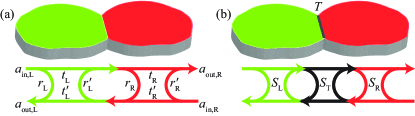
Figure 3: (Online version in colour.) Scattering amplitudes and their relation by reflection and transmission blocks of the scattering matrix, for the coupled-resonator geometry considered in section VIII–section X. In (b), a finite transparency $T$ of the interface is taken into account. See also hsqoptics ; yoo ; hsrmt .

VIII.1 Scattering matrix

Denoting the scattering matrices of the two resonators as

$$S_{L}=\left(\begin{array}[]{cc}r_{L}&t_{L}^{\prime}\\ t_{L}&r_{L}^{\prime}\\ \end{array}\right),\quad S_{R}=\left(\begin{array}[]{cc}r_{R}&t_{R}^{\prime}\\ t_{R}&r_{R}^{\prime}\\ \end{array}\right),$$ (38)

the scattering matrix $S=S_{L}\circ S_{R}$ of the composed system is given by

$$\left(\begin{array}[]{cc}r_{L}&t_{L}^{\prime}\\ t_{L}&r_{L}^{\prime}\end{array}\right)\circ\left(\begin{array}[]{cc}r_{R}&t_{R}^{\prime}\\ t_{R}&r_{R}^{\prime}\end{array}\right)$$ (43)

$$=\left(\begin{array}[]{cc}r_{L}+t_{L}^{\prime}\frac{1}{1-r_{R}r_{L}^{\prime}}r_{R}t_{L}&t_{L}^{\prime}\frac{1}{1-r_{R}r_{L}^{\prime}}t_{R}^{\prime}\\ t_{R}\frac{1}{1-r_{L}^{\prime}r_{R}}t_{L}&r_{R}^{\prime}+t_{R}\frac{1}{1-r_{L}^{\prime}r_{R}}r_{L}^{\prime}t_{R}^{\prime}\end{array}\right).$$ (46)

$\mathcal{PT}$ symmetry follows if the scattering matrices are related by $S_{R}=\mathcal{PT}[S_{L}]$, with this operation specified in equation (26), while $\mathcal{PTT}^{\prime}$ symmetry is realized if the scattering matrices are related by $S_{R}=\mathcal{PTT^{\prime}}[S_{L}]$, as specified in equation (32).

This construction can be amended to include an interface of finite transparency $T$, with the scattering matrix, e.g., specified by

$$S_{T}=\left(\begin{array}[]{cc}-\sqrt{1-T}&i\sqrt{T}\\ i\sqrt{T}&-\sqrt{1-T}\\ \end{array}\right).$$ (47)

The total scattering matrix of the system is then given by $S=S_{L}\circ S_{T}\circ S_{R}$.

VIII.2 Quantization conditions and spectral constraints

With equation (46) the scattering quantization condition (37) becomes

$${\rm det}\,[r_{L}^{\prime}(\omega)r_{R}(\omega)-\openone]=0.$$ (48)

For a $\mathcal{PT}$-symmetric system obeying equation (V.1) this condition takes the form

$${\rm det}\,(r_{L}^{\prime}(\omega)-[r_{L}^{\prime}(\omega^{*})-t_{L}(\omega^{*})r_{L}^{-1}(\omega^{*})t_{L}^{\prime}(\omega^{*})]^{*})=0,$$ (49)

while for a $\mathcal{PTT}$-symmetric system obeying equation (V.2) this gives

$${\rm det}\,(r_{L}^{\prime}(\omega)-[r_{L}^{\prime}(\omega^{*})-t_{L}(\omega^{*})r_{L}^{-1}(\omega^{*})t_{L}^{\prime}(\omega^{*})]^{\dagger})=0.$$ (50)

For a closed system the scattering matrices reduce to the reflection blocks $S_{L}(\omega)=r_{L}^{\prime}(\omega)$ and $S_{R}(\omega)=r_{R}(\omega)$, while the transmission vanishes. In the case of $\mathcal{PT}$ symmetry, with $r_{R}(\omega)=\{[r_{L}^{\prime}(\omega^{*})]^{-1}\}^{*}$, equation (49) assumes the form

$${\rm det}\,(r_{L}^{\prime}(\omega)-[r_{L}^{\prime}(\omega^{*})]^{*})=0,$$ (51)

which entails the constraints (12). On the real frequency axis, this reduces to the condition ${\rm det}\,{\rm Im}\,r_{L}^{\prime}(\omega)=0.$ Analogous observations also hold for closed $\mathcal{PTT}^{\prime}$-symmetric resonators, for which the quantization condition (50) becomes

$${\rm det}\,(r_{L}^{\prime}(\omega)-[r_{L}^{\prime}(\omega^{*})]^{\dagger})=0.$$ (52)

Under inclusion of a semitransparent interface, similar conditions can be derived from the general expression

$${\rm det}\,\left[S_{T}\left(\begin{array}[]{cc}r_{L}^{\prime}&0\\ 0&r_{R}\\ \end{array}\right)-\openone\right]=0.$$ (53)

These scattering quantization conditions can all be interpreted as conditions for constructive interference upon return to the interface between the two parts of the resonator. The analogous conditions for perfectly absorbed states follow from the replacement $\omega\to\omega^{*}$.

IX Effective Models

The coupled-resonator geometry allows to make contact to well-studied standard descriptions of multiple scattering beenakkerreview ; fyodorovsommers ; fyodsomeffs ; andreev ; schomerusjacquod . This leads to effective models of complex wave dynamics in systems with $\mathcal{PT}$ and $\mathcal{PTT}^{\prime}$ symmetry, which we first formulate in the energy domain hsrmt , and then in the time domain birchallweyl .

IX.1 Effective Hamiltonians

We first employ the Hamiltonian approach to multiple scattering beenakkerreview ; fyodorovsommers . The hermitian part of the dynamics in the absorbing resonator is captured by a hermitian $M\times M$-dimensional matrix $H$. We assume $M\gg 1$ and denote the level spacing in the energy range of interest as $\Delta$. Loss with absorption rate $\mu$ is modeled by adding a non-hermitian term $-i\mu\openone$, while gain with a matching rate is obtained by inverting the sign of $\mu$. We also specify an $N\times M$-dimensional coupling matrix $V$ between the $M$ internal modes and $N$ scattering states. This matrix can be chosen to satisfy $V^{T}V={\rm diag}{(v_{m})}$, where $N$ finite entries $v_{m}=\Delta M/\pi$ describe the open channels, while $M-N$ entries $v_{m}=0$ describe the closed channels. The $N\times N$-dimensional scattering matrix of the absorbing resonator is then given by

$$S_{L}(\omega)=1-2iV(\omega-i\mu-H+iV^{T}V)^{-1}V^{T}.$$ (54)

Thus, the leakage from the system effectively adds an additional non-hermitian term $-iV^{T}V$ to the Hamiltonian. For $\mathcal{PT}$ symmetry the scattering matrix of the amplifying resonator follows as hsrmt

$$S_{R}(\omega)=[S_{L}^{-1}(\omega^{*})]^{*}=1-2iV(\omega+i\mu-H^{*}+iV^{T}V)^{-1}V^{T}.$$ (55)

We also include a semitransparent interface, with scattering matrix (47). For a closed system, the scattering quantization condition (53) can then be rearranged into an eigenvalue problem ${\rm det}\,(\omega-{\cal H})=0$ with effective Hamiltonian hsrmt

$${\cal H}=\left(\begin{array}[]{cc}H-i\mu&\Gamma\\ \Gamma&H^{*}+i\mu\\ \end{array}\right).$$ (56)

Here $\Gamma={\rm diag}\,(\gamma_{m})$ is a real positive semi-definite coupling matrix related to $V^{T}V$, but with the $N$ non-vanishing entries $\gamma_{m}=[\sqrt{T}/(1+\sqrt{1-T})]\Delta M/\pi\equiv\gamma$ modified to account for the finite transparency $T$ of the interface.

The effective Hamiltonian obeys the relation $\mathcal{PT}[\mathcal{H}]=\sigma_{x}\mathcal{H}^{*}\sigma_{x}=\mathcal{H}$. In a $\mathcal{PT}$-symmetric basis the secular equation ${\rm det}\,(\omega-{\cal H})=0$ then takes the form of a polynomial with real coefficients, which guarantees that the eigenvalues are either real or occur in complex-conjugate pairs, as required by equation (12).

Analogous considerations apply to $\mathcal{PTT}^{\prime}$-symmetric systems hsrmt ; birchallrmt . The scattering matrix of the right resonator then changes to

$$S_{R}(\omega)=[S_{L}^{-1}(\omega^{*})]^{\dagger}=1-2iV(\omega+i\mu-H+iV^{T}V)^{-1}V^{T},$$ (57)

and the effective Hamiltonian of the closed system takes the form

$${\cal H}=\left(\begin{array}[]{cc}H-i\mu&\Gamma\\ \Gamma&H+i\mu\\ \end{array}\right).$$ (58)

We then have $\mathcal{PTT}^{\prime}[\mathcal{H}]=\sigma_{x}\mathcal{H}^{\dagger}\sigma_{x}=\mathcal{H}$, which again guarantees the required spectral constraints.

While Hamiltonians with these symmetries could simply be stipulated, the derivation of the specific manifestations (56) and (58) reveals further constraints dictated by the coupled-resonator geometry. In particular, the coupling is only physical if the matrix $\Gamma$ is positive semidefinite. These Hamiltonians bear a striking resemblance to models of mesoscopic superconductivity beenakkerreview ; melsen .

IX.2 Quantum maps

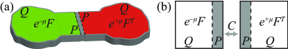
Figure 4: (Online version in colour.) Interpretation of the $\mathcal{PT}$-symmetric quantum map (63), which translates the resonator dynamics in (a) to a stroboscopic evolution in two coupled Hilbert spaces (b). For the $\mathcal{PTT}^{\prime}$-symmetric map (68), $F^{T}$ is replaced by $F$. See also birchallweyl .

Alternatively, one can set up effective descriptions in the time domain birchallweyl . For $\mathcal{PT}$ symmetry this sets out by writing the scattering matrices as fyodsomeffs ; andreev ; schomerusjacquod

$$S_{L}(\omega) =WF[\exp(-i\omega\tau+\mu)-QF]^{-1}W^{T},$$ (59a)

$$S_{R}(\omega) =WF^{T}[\exp(-i\omega\tau-\mu)-QF^{T}]^{-1}W^{T},$$ (59b)

where $F$ is an $M\times M$-dimensional unitary matrix which can be thought to describe the stroboscopic time evolution between successive scattering events off the resonator walls. The transfer across the interface between the two resonators is again described by an $N\times M$-dimensional coupling matrix $W$. However, the combination $P=W^{T}W$ now projects the wave function onto the interface, such that ${\rm rank}\,P=N$ is the number of channels connecting the resonators, while $Q=\openone_{M}-P$ is the complementary projector onto the resonator wall (${\rm rank}\,Q=M-N$). The stated frequency dependence corresponds to stroboscopic scattering with fixed rate $\tau^{-1}$; the variable $\omega$ thus plays the role of a quasienergy. The parameter $\mu\geq 0$ again determines the absorption and amplification rate. For the passive system ($\mu=0$), the scattering matrices are unitary, which corresponds to the hermitian limit of the problem.

With these specifications, and including a semitransparent interface parameterized by $\alpha\equiv\sqrt{\sqrt{R}+i\sqrt{T}}$, the quantization condition (53) is equivalent to the eigenvalue problem

$${\cal F}\psi_{n}=\lambda_{n}\psi_{n},\quad\lambda_{n}=\exp(-i\omega_{n}\tau)$$ (60)

for the quantum map

$${\cal F} =\sqrt{C}\left(\begin{array}[]{cc}e^{-\mu}F&0\\ 0&e^{\mu}F^{T}\\ \end{array}\right)\sqrt{C},$$ (63)

$$\quad\sqrt{C} =\left(\begin{array}[]{cc}\mathrm{Re}\,\alpha\,P+Q&-i\mathrm{Im}\,\alpha\,P\\ -i\mathrm{Im}\,\alpha\,P&\mathrm{Re}\,\alpha\,P+Q\\ \end{array}\right)$$ (66)

where we symmetrized the coupling

$$C=\sqrt{C}\sqrt{C}=\left(\begin{array}[]{cc}\sqrt{R}P+Q&-iP\sqrt{T}\\ -iP\sqrt{T}&\sqrt{R}P+Q\\ \end{array}\right).$$ (67)

The $2M\times 2M$ dimensional matrix ${\cal F}$ can be interpreted as a stroboscopic time evolution operator acting on $2M$-dimensional vectors $\psi=\binom{\psi_{L}}{\psi_{R}}$, where $\psi_{L}$ and $\psi_{R}$ give the wave amplitude in the absorbing and amplifying subsystem, respectively. This is illustrated in figure 4. The $\mathcal{PT}$ symmetry of the quantum map manifests itself in the relation ${\cal F}=\sigma_{x}[{\cal F}^{-1}]^{*}\sigma_{x}$, which parallels the symmetry (26) for the scattering matrix.

Analogously, $\mathcal{PTT}^{\prime}$ symmetry results in the quantum map

$${\cal F}=\sqrt{C}\left(\begin{array}[]{cc}e^{-\mu}F&0\\ 0&e^{\mu}F\\ \end{array}\right)\sqrt{C}.$$ (68)

This obeys the symmetry ${\cal F}=\sigma_{x}[{\cal F}^{-1}]^{\dagger}\sigma_{x}$, which parallels equation (32).

The spectral properties associated with these symmetries are now embodied in the secular equation $s(\lambda)=\rm{det}\,({\cal F}-\lambda)=0$, which exhibits the mathematical property of self-inversiveness selfinverse2 :

$$s(1/\lambda^{*})=[\lambda^{-2M}s(\lambda)]^{*}s(0),$$ (69)

where $s(0)=\mathrm{det}\,\mathcal{F}=(\mathrm{det}\,F)^{2}$. For each eigenvalue $\lambda_{n}$, we are thus guaranteed to find the eigenvalue $\lambda_{\bar{n}}=[\lambda_{n}^{-1}]^{*}=\exp(-i\omega_{n}^{*}\tau)$, which recovers the constraint (12).

X Mesoscopic energy and times scales

In mesoscopic physics, a large range of spectral, thermodynamic and transport phenomena are fully characterized by a few universal time and energy scales beenakkerreview ; datta ; altlandthouless . We now have all the tools to make contact to these concepts and provide a phenomenological description of the effects of multiple scattering on the spectral features of the considered coupled resonators. These effects generally set in when a large number $M\gg 1$ of internal modes in an energy range $M\Delta$ is mixed by scattering with a characteristic time scale $\tau=\hbar/M\Delta$ that is much less than the dwell time in the amplifying or absorbing regions, $\tau\ll t_{\mathrm{dwell}}$. The coupling strength between these regions is characterized by the associated Thouless energy $E_{T}=\hbar/t_{\mathrm{dwell}}\approx NT\Delta$, which can be small or large compared to the level spacing $\Delta$, depending on the value of the dimensionless conductance $g=NT$ of the interface. Non-hermiticity adds the new scale $\mu$, whose interplay with the other scales determines the transition from real to complex eigenvalues.

In the mesoscopic regime of $M\gg N\gg 1$ this transition can be expected to be universal, with the features only depending on $M/N\gg 1$, $M\gg 1$, and $T$, which we consider fixed by the geometry, as well as the variable $\mu$. The transition can then be investigated by combining the effective models set up in the previous section with random-matrix theory beenakkerreview ; haake ; mehta , thus, ensembles of Hamiltonians $H$ (usually composed with random Gaussian matrix elements) or time-evolution operators $F$ (distributed according to a Haar measure) which are only constrained by the symmetries of the problem. Closer inspection identifies two natural scenarios hsrmt ; birchallrmt , described in the following two subsections, and a semiclassical source of corrections to random-matrix theory, discussed thereafter birchallweyl . The interplay of the various time and energy scales is illustrated in figure 5.

X.1 Systems with coupling-driving level crossings

In ordinary optics with exact $\mathcal{T}^{\prime}$ symmetry, systems with $\mathcal{PT}$ symmetry also display $\mathcal{PTT}^{\prime}$ symmetry. The internal Hamiltonian $H=H^{*}=H^{T}$ is then real and symmetric, and the effective Hamiltonians (56) and (58) coincide. (Analogously, $F=F^{T}$, so that the quantum maps (63) and (68) coincide as well.) Switching to a parity-invariant basis one then finds

$${\cal H}_{\cal P}=\left(\begin{array}[]{cc}H+\Gamma&i\mu\\ i\mu&H-\Gamma\\ \end{array}\right),$$ (70)

which reveals the emerging $\mathcal{T}$ symmetry in the hermitian limit. The same structure arises for systems with magneto-optical effects which only display $\mathcal{PTT}^{\prime}$. For both cases, at $\mu=0$ the system decouples into two independent sectors. For $T=0$ the level sequences of these sectors coincide. For very weak coupling ($T\ll 1/N\equiv T_{c}$, thus $g\ll 1$) the degeneracy is slightly lifted, and one can apply almost-degenerate perturbation theory to identify the scale $\mu\approx N\sqrt{T}\Delta/2\pi$ at which typical eigenvalues turn complex. As $T$ exceeds $1/N\equiv T_{c}$ ($g>1$), however, the levels of the original sequences cross, and when one then increases $\mu$ the bifurcations to complex eigenvalues occur between levels that were originally non-degenerate. In this regime, a macroscopic fraction of complex eigenvalues appears on a coupling-independent scale $\mu\approx\mu_{0}\equiv\sqrt{N}\Delta/2\pi$.

X.2 Systems with coupling-driving avoided crossings

For systems with $\mathcal{PT}$ symmetry but broken $\mathcal{T}^{\prime}$ symmetry, the parity basis does not partially diagonalize the effective Hamiltonian. At $\mu=T=0$, one still starts from two degenerate level sequences, but these interact as $T$ is increased, and instead of level crossings one observes level repulsion. In this case the crossover to a complex spectrum appears at $\mu\approx\sqrt{NT}\Delta/2\pi$ and thus is always coupling dependent.

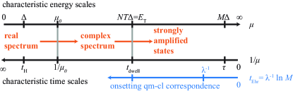
Figure 5: (Online version in colour.) Sketch of the energy and time scales governing the spectral features of $\mathcal{PT}$-symmetric resonators with separate $\mathcal{T}^{\prime}$ invariance (no magneto-optical effects), as hermiticity is broken with absorption and amplification rate $\mu$. This universal picture holds under the assumption of complex wave dynamics ($M\gg N,NT\gg 1$), where $M=\hbar/\tau\Delta$ is the number of internal modes mixed by multiple scattering with scattering time $\tau$ and $N$ is the number of channels coupling the resonators, with transparency $T$. Here $\Delta$ is the mean level spacing, $t_{\rm H}=\hbar/\Delta$ the Heisenberg time, and $E_{T}=\hbar/t_{\rm dwell}=NT\Delta$ the Thouless energy associated with the dwell time $t_{\rm dwell}$ in each resonator. The critical rate at which eigenvalues turn complex is $\mu_{0}=\sqrt{N}\Delta/2\pi$. When the Ehrenfest time $t_{\rm Ehr}=\lambda^{-1}\ln M$ (with Lyapunov exponent $\lambda$) becomes comparable to the dwell time $t_{\rm dwell}$ quantum-to classical-correspondence sets in and suppresses multiple scattering, which reduces the number of strongly amplified states. See also hsrmt ; birchallweyl .

X.3 Growth and decay rates in the semiclassical limit

In the semiclassical limit of large $M$ at fixed $M/N$ the results above imply that the crossover to a complex spectrum appears at a vanishingly small rate $\mu\ll E_{T}$. Keeping $\mu/E_{T}$ in this limit fixed and finite, the real phase is thus completely destroyed, and the focus turns to the typical decay and growth rates encoded in the imaginary parts ${\rm Im}\,\omega_{n}$ of the complex eigenvalues. Numerical sampling of the random-matrix ensembles suggests that the distribution $P({\rm Im}\,\omega_{n}/\mu;\mu/E_{T})$ attains a stationary limit for $M\gg 1$ hsrmt ; birchallweyl ; birchallrmt . At $\mu\gtrsim E_{T}$, one then finds a finite fraction of strongly amplified states with ${\rm Im}\,\omega_{n}\approx\mu$, thus, a large number of candidate lasing states. However, the fraction of these states is reduced when one takes dynamical effects into account birchallweyl . One then finds that the strongly amplified states are supported by the classical repeller in the amplifying parts of the system, whose fractal dimension $d_{H}$ is more and more resolved as the phase space resolution $h\propto 1/M$ increases in the semiclassical limit. This phenomenon can be characterized by the Ehrenfest time $t_{\rm Ehr}=\lambda^{-1}\ln M$, where $\lambda$ the Lyapunov exponent in the classical system. If $t_{\rm Ehr}>t_{\rm dwell}$, the wave dynamics become quasi-deterministic, and multiple scattering is reduced. The fraction of strongly amplified states then follows a fractal Weyl law (a power law in $h$ with non-integer exponent), a phenomenon which was previously observed for passive quantum systems with finite leakage through ballistic openings fractalweyl1 ; fractalweyl3 .

XI Summary and outlook

In summary, the scattering approach proves useful to describe general features of non-hermitian optical systems with $\mathcal{PT}$ and $\mathcal{PTT}^{\prime}$ symmetry. In particular, the approach fully accounts for complications that arise beyond one dimension (a choice of non-equivalent geometric and time-reversal symmetries, the possibility of magneto-optical effects with a finite external vector potential, and multiple scattering), as well as additional leakage which turns the symmetry of bound states into a relation between quasibound and perfectly absorbed states. These effects can be captured in effective model Hamiltonians and time evolution operators, which help to identify the mesoscopic energy and time scales that govern the spectral features of a broad class of systems. The construction of these models exposes physical constraints that go beyond the mere symmetry requirements.

The models formulated here can be adapted to include, e.g., inhomogeneities in the gain, dissipative magneto-optical effects, leakage, or other symmetry-breaking effects birchallrmt . Furthermore, the construction of symmetric resonators from two subsystems can be extended to include more elements, such as they occur in periodic or disordered arrays. This bridges to models of higher-dimensional diffusive or Anderson-localized dynamics west . The models can also be generalized to include symplectic time-reversal symmetries (with $\mathcal{T}^{2}=-1$), chiral symmetries, or particle-hole symmetries (as the $\mathcal{CT}$ symmetry obeyed by mesoscopic superconductors), for which the consequences on the scattering matrix and effective Hamiltonians are well known in the hermitian case beenakkerreview ; altlandzirnbauer ; melsen . Some of these effects have optical analogues; e.g., phase-conjugating mirrors induce effects similar to Andreev reflection in mesoscopic superconductivity but result in a non-hermitian Hamiltonian beenakkerphase . Finally we note that the scattering approach also offers a wide range of analytical and numerical methods which allow to efficiently study individual systems datta .

I thank Christopher Birchall for fruitful collaboration on Refs. birchallweyl ; birchallrmt , which form the basis of some of the material reviewed here, as well as Uwe Günther for fruitful discussions concerning the role of symmetries.

References

- (1) Bender, C. M. & Boettcher, S. 1998 Real Spectra in Non-Hermitian Hamiltonians Having PT Symmetry Phys. Rev. Lett. 80, 5243–5246. (doi:10.1103/PhysRevLett.80.5243)
- (2) Bender, C. M. 2007 Making sense of non-Hermitian Hamiltonians. Rep. Prog. Phys. 70, 947–1018. (doi:10.1088/0034-4885/70/6/R03)
- (3) Mostafazadeh, A. 2010 Pseudo-Hermitian representation of quantum mechanics. Int. J. Geom. Meth. Mod. Phys. 7, 1191–1306. (doi:10.1142/S0219887810004816)
- (4) El-Ganainy, R., Makris, K. G., Christodoulides, D. N. & Musslimani, Z. H. 2007 Theory of coupled optical PT-symmetric structures. Opt. Lett. 32, 2632–2634. (doi:10.1364/OL.32.002632)
- (5) Makris, K. G., El-Ganainy, R., Christodoulides, D. N. & Musslimani, Z. H. 2008 Beam Dynamics in PT Symmetric Optical Lattices. Phys. Rev. Lett. 100, 103904. (doi:10.1103/PhysRevLett.100.103904)
- (6) Musslimani, Z. H., Makris, K. G., El-Ganainy, R. & Christodoulides, D. N. 2008 Optical Solitons in PT Periodic Potentials. Phys. Rev. Lett. 100, 030402. (doi:10.1103/PhysRevLett.100.030402)
- (7) Guo, A., Salamo, G. J., Duchesne, D., Morandotti, R., Volatier-Ravat, M., Aimez, V., Siviloglou, G. A. & Christodoulides, D. N. 2009 Observation of PT-Symmetry Breaking in Complex Optical Potentials. Phys. Rev. Lett. 103, 093902. (doi:10.1103/PhysRevLett.103.093902)
- (8) Rüter, C. E., Makris, K. G., El-Ganainy, R., Christodoulides, D. N., Segev, M. & Kip, D. 2010 Observation of parity-time symmetry in optics. Nature Phys. 6, 192–195. (doi:10.1038/nphys1515)
- (9) Longhi, S. 2009 Bloch Oscillations in Complex Crystals with PT Symmetry. Phys. Rev. Lett. 103, 123601. (doi:10.1103/PhysRevLett.103.123601)
- (10) Ramezani, H., Kottos, T., El-Ganainy, R. & Christodoulides, D. N. 2010 Unidirectional nonlinear PT-symmetric optical structures. Phys. Rev. A 82, 043803. (doi:10.1103/PhysRevA.82.043803)
- (11) Longhi, S. 2011 Invisibility in PT-symmetric complex crystals. J. Phys. A: Math. Theor. 44, 485302. (doi:10.1088/1751-8113/44/48/485302)
- (12) Lin, Z., Ramezani, H., Eichelkraut, T., Kottos, T., Cao, H. & Christodoulides, D. N. 2011 Unidirectional Invisibility Induced by PT-Symmetric Periodic Structures. Phys. Rev. Lett. 106, 213901. (doi:10.1103/PhysRevLett.106.213901)
- (13) Schomerus, H. 2010 Quantum Noise and Self-Sustained Radiation of PT-Symmetric Systems. Phys. Rev. Lett. 104, 233601. (doi:10.1103/PhysRevLett.104.233601)
- (14) Longhi, S. 2010 PT-symmetric laser absorber. Phys. Rev. A 82, 031801(R). (doi:10.1103/PhysRevA.82.031801)
- (15) Chong, Y. D., Ge, L. & Stone, A. D. 2011 PT-Symmetry Breaking and Laser-Absorber Modes in Optical Scattering Systems. Phys. Rev. Lett. 106, 093902. (doi:10.1103/PhysRevLett.106.093902)
- (16) Ge, L., Chong, Y. D. & Stone, A. D. 2012 Conservation relations and anisotropic transmission resonances in one-dimensional PT-symmetric photonic heterostructures. Phys. Rev. A 85, 023802. (doi:10.1103/PhysRevA.85.023802)
- (17) Yoo, G., Sim, H.-S. & Schomerus, H. 2011 Quantum noise and mode nonorthogonality in non-Hermitian PT-symmetric optical resonators. Phys. Rev. A 84, 063833. (doi:10.1103/PhysRevA.84.063833)
- (18) Schomerus, H and Yunger Halpern, N. 2013 Parity anomaly and Landau-level lasing in strained photonic honeycomb lattices. Phys. Rev. Lett. 110, 013903. (doi:10.1103/PhysRevLett.110.013903)
- (19) Vahala, K. J. 2003 Optical microcavities. Nature 424, 839–846. (doi:10.1038/nature01939)
- (20) Beenakker, C. W. J. 1997 Random-matrix theory of quantum transport. Rev. Mod. Phys. 69, 731–808. (doi:10.1103/RevModPhys.69.731)
- (21) Datta, S. 1997 Electronic Transport in Mesoscopic Systems. Cambridge, UK: Cambridge University Press.
- (22) Altland, A. & Zirnbauer, M. R. 1997 Nonstandard symmetry classes in mesoscopic normal-superconducting hybrid structures. Phys. Rev. B 55, 1142–1161. (doi:10.1103/PhysRevB.55.1142)
- (23) Haake, F. 2010 Quantum signatures of chaos, 3rd ed. Berlin: Springer.
- (24) Fyodorov, Y. V. & Sommers, H.-J. 1997 Statistics of resonance poles, phase shifts and time delays in quantum chaotic scattering: Random matrix approach for systems with broken time-reversal invariance. J. Math. Phys. 38, 1918–1981. (doi:10.1063/1.531919)
- (25) Onsager, L. 1931 Reciprocal relations in irreversible processes. I. Phys. Rev. 37, 405. (doi:10.1103/PhysRev.37.405)
- (26) Schomerus, H. 2011 Universal routes to spontaneous PT-symmetry breaking in non-Hermitian quantum systems. Phys. Rev. A 83, 030101(R). (doi:10.1103/PhysRevA.83.030101)
- (27) Birchall, C. & Schomerus, H. 2012 Fractal Weyl laws for amplified states in PT-symmetric resonators. arxiv:1208.2259
- (28) Birchall, C. & Schomerus, H. 2012 Random-matrix theory of amplifying and absorbing resonators with PT or PTT′ symmetry. preprint.
- (29) Cannata, F., Dedonder, J.-P. & Ventura, A. 2007 Scattering in PT-symmetric quantum mechanics. Ann. Phys. (N.Y.) 322, 397–433. (doi:10.1016/j.aop.2006.05.011)
- (30) Berry, M. V. 2008 Optical lattices with PT symmetry are not transparent. J. Phys. A: Math. Theor. 41, 244007. (doi:10.1088/1751-8113/41/24/244007)
- (31) Jones, H. F. 2007 Scattering from localized non-Hermitian potentials. Phys. Rev. D 76, 125003. (doi:10.1103/PhysRevD.76.125003)
- (32) Magnea, U. 2008 Random matrices beyond the Cartan classification. J. Phys. A: Math. Theor. 41, 045203 (doi:10.1088/1751-8113/41/4/045203)
- (33) Melsen, J. A., Brouwer, P. W., Frahm, K. M. & Beenakker, C. W. J. 1996 Induced superconductivity distinguishes chaotic from integrable billiards. Europhys. Lett. 35, 7. (doi:10.1209/epl/i1996-00522-9)
- (34) Chong, Y. D., Ge, L., Cao, H. & Stone, A. D. 2010 Coherent Perfect Absorbers: Time-Reversed Lasers. Phys. Rev. Lett. 105, 053901. (doi:10.1103/PhysRevLett.105.053901)
- (35) Fyodorov, Y. V. & Sommers, H.-J. 2000 Spectra of random contractions and scattering theory for discrete-time systems. JETP Lett. 72, 422–426. (doi:10.1134/1.1335121)
- (36) Jacquod, Ph., Schomerus, H. & Beenakker, C. W. J. 2003 Quantum Andreev Map: A Paradigm of Quantum Chaos in Superconductivity. Phys. Rev. Lett. 90, 207004. (doi:10.1103/PhysRevLett.90.207004)
- (37) Schomerus, H. & Jacquod, P. 2005 Quantum-to-classical correspondence in open chaotic systems. J. Phys. A: Math. Gen. 38, 10663-10682. (doi:10.1088/0305-4470/38/49/013)
- (38) Haake, F., Kuś, M., Sommers, H.-J., Schomerus, H. & Życzkowski, K. 1996 Secular determinants of random unitary matrices. J. Phys. A: Math. Gen. 29, 3641–3658. (doi:10.1088/0305-4470/29/13/029)
- (39) Altland, A., Gefen, Y. & Montambaux, G. 1996 What is the Thouless Energy for Ballistic Systems? Phys. Rev. Lett. 76, 1130–1133. (doi:10.1103/PhysRevLett.76.1130)
- (40) Mehta, M. L. 2004 Random Matrices, 3rd ed. New York, NY: Elsevier.
- (41) Lu, W. T., Sridhar, S. & Zworski, M. 2003 Fractal Weyl Laws for Chaotic Open Systems. Phys. Rev. Lett. 91, 154101. (doi:10.1103/PhysRevLett.91.154101)
- (42) Schomerus, H. & Tworzydło, J. 2004 Quantum-to-Classical Crossover of Quasibound States in Open Quantum Systems. Phys. Rev. Lett. 93, 154102. (doi:10.1103/PhysRevLett.93.154102)
- (43) West, C. T., Kottos, T. & Prosen, T. 2010 PT-Symmetric Wave Chaos. Phys. Rev. Lett. 104, 054102. (doi:10.1103/PhysRevLett.104.054102)
- (44) Paasschens, J. C. J., de Jong, M. J. M., Brouwer, P. W. & Beenakker, C. W. J. 1997 Reflection of light from a disordered medium backed by a phase-conjugating mirror. Phys. Rev. A 56, 4216–4228. (doi:10.1103/PhysRevA.56.4216)