Approximability of convex bodies and volume entropy in Hilbert geometry

Abstract.

The approximability of a convex body is a number which measures the difficulty in approximating that convex body by polytopes. In the interior of a convex body one can define its Hilbert geometry. We prove on the one hand that the volume entropy is twice the approximability for a Hilbert geometry in dimension two end three, and on the other hand that in higher dimensions it is a lower bound of the entropy. As a corollary we solve the volume entropy upper bound conjecture in dimension three and give a new proof in dimension two from the one given in [BBV10]. Moreover, our method allows us to prove the existence of Hilbert geometries with intermediate volume growth one the one hand, and that in general the volume entropy is not a limit on the other hand.

Introduction and statement of results

Hilbert geometries are all the metric spaces obtained by defining the so-called Hilbert distance on open bounded convex sets in ${\mathbb{R}}^{n}$. The definition of this distance uses cross-ratios in the same way as in Klein projective model of the hyperbolic geometry [Hil71]. These metric spaces are actually length space whose structure is defined by a Finsler metric which is Riemannian if and only if the underlying open bounded convex set is an ellipsoid [Kay67].

These geometries have attracted a lot of interest see for example the works of Y. Nasu [Nas61], W. Goldmann [Gol90], P. de la Harpe [dlH93], A. Karlsson and G. Noskov [KN02], Y. Benoist [Ben03, Ben06], T. Foertsch and A. Karlsson [FK05], I. Kim [Kim05], B. Colbois, C. Vernicos and P. Verovic [CVV04, CVV06], B. Lins and R. Nussbaum [LN08], A. Borisenko and E. Olin [BO08, BO11], B. Lemmens and C. Walsh [LW11], C. Vernicos [Ver09, Ver11, Ver13], L. Marquis [Mar12], M. Crampon and L. Marquis [CM14], D. Cooper, D. Long and S. Tillman [CLT]), X. Nie [Nie] and the Handbook of Hilbert geometry [Hbk14].

The present paper focuses on the volume growth of these geometries and more specifically on the volume entropy.

Let $\Omega$ be a bounded open convex set in ${\mathbb{R}}$ endowed with its Hilbert geometry. If we consider the Busemann volume ${\rm Vol}_{\Omega}$ and denote by $B_{\Omega}(p,r)$ the metric ball of radius $r$ centred at the point $p\in\Omega$, then the lower and upper volume entropies of $\Omega$ will be defined respectively by

(1) $$\operatorname{\underline{Ent}}(\Omega)=\liminf_{r\to+\infty}\dfrac{\ln\bigl{(}{\rm Vol}_{\Omega}(B_{\Omega}(p,r)\bigr{)}}{r}\text{, and }\\ \operatorname{\overline{Ent}}(\Omega)=\limsup_{r\to+\infty}\dfrac{\ln\bigl{(}{\rm Vol}_{\Omega}(B_{\Omega}(p,r)\bigr{)}}{r}\text{.}$$

When the two limits coincide we denote their common limit by $\operatorname{Ent}(\Omega)$ and call it the volume entropy of $\Omega$.

Let us stress out that in this definition the upper and lower volume entropy of $\Omega$ do not depend on the base point $p$ and are actually projective invariant attached to $\Omega$.

The question we address in this essay is twofold. On the one hand it is an investigation of the existence of an analogue, for all Hilbert geometries, of the relation between the volume entropy and the Hausdorff dimension of the radial limit set on the universal cover of a compact Riemannian manifold with non-positive curvature. On the other hand we focus on the volume entropy upper bound conjecture which states that if $\Omega$ is an open and bounded convex subset of ${\mathbb{R}}^{n}$, then $\operatorname{\overline{Ent}}(\Omega)\leq n-1$. To put our work into perspective let us recall the main related results.

The first one is a complete answer to the conjecture in the two-dimensional case by G. Berck, A. Bernig and C. Vernicos in [BBV10], where the authors actually obtained an upper bound as a function of $d$, the upper Minkowski dimension (or ball-box dimension) of the set of extreme points of $\Omega$, namely

(2) $$\operatorname{\overline{Ent}}(\Omega)\leq\frac{2}{3-d}\leq 1.$$

The second result is a more precise statement with respect to the asymptotic volume growth of balls. It involves another projective invariant introduced by G. Berck, A. Bernig and C. Vernicos in the introduction of [BBV10] called the centro-projective area of $\Omega$, and defined by

(3) $$\mathcal{A}_{p}(\Omega):=\int_{\partial\Omega}\frac{\sqrt{k(x)}}{\langle n(x),x-p\rangle^{\frac{n-1}{2}}}\left(\frac{2(\alpha x)}{1+a(x)}\right)^{\frac{n-1}{2}}\ dA(x),$$

where for any $x\in\partial\Omega$, $k(x)$ is the Gauss curvature, $n(x)$ the outward normal and $\alpha(x)>0$ is the function defined by $p-\alpha(x)(x-p)\in\partial\Omega$. Let us recall here that both $k$ and $n$ are defined almost everywhere as Alexandroff’s theorem states [Ale39].

Now, the Second Main Theorem of G. Berck, A. Bernig and C. Vernicos in [BBV10] — which encloses former results given by B. Colbois and P. Verovic in [CV04] — asserts that in case $\partial\Omega$ is $C^{1,1}$ we have

(4) $$\lim_{r\to+\infty}\frac{{\rm Vol}_{\Omega}B_{\Omega}(p,r)}{\sinh^{n-1}r}=\frac{1}{n-1}\mathcal{A}_{p}(\Omega)\neq 0$$

and $\operatorname{Ent}(\Omega)=n-1$ is a limit. Moreover, without any assumption on $\Omega$ we have $\operatorname{\underline{Ent}}(\Omega)\geq n-1$ whenever $\mathcal{A}_{p}(\Omega)\neq 0$.

The third one — which is also a rigidity result — requires stronger assumptions about $\Omega$: it has to be divisible, meaning that it admits a compact quotient, and its Hilbert metric has to be hyperbolic in the sense of Gromov, which implies its boundary is $C^{1}$ and strictly convex by Y. Benoist in [Ben03]. Let us stress out that the Hilbert metric on such an $\Omega$ is the hyperbolic one if and only if $\Omega$ has a $C^{1,1}$ boundary, and that its volume entropy is positive since hyperbolicity implies the non-vanishing of the Cheeger constant (see Theorem 1.5 in B. Colbois and C. Vernicos [CV07]). A result by M. Crampon (see [Cra09]) states that for a divisible open bounded convex set $\Omega$ in ${\mathbb{R}}^{n}$ whose boundary is $C^{1}$ we have $\operatorname{Ent}(\Omega)\leq n-1$ with equality if and only if $\Omega$ is an ellipsoid.

In the present paper we link the volume entropy to another invariant associated with a convex body, called the approximability. This name was introduced by Schneider and Wieacker in [SW81]. The approximability measures in some sense how well a convex set can be approximated by polytopes. More precisely, let $N(\varepsilon,\Omega)$ be the smallest number of vertices of a polytope whose Hausdorff distance to $\Omega$ is less than $\varepsilon>0$. Then the lower and upper approximability of $\Omega$ are defined by

(5) $$\underline{a}(\Omega):=\liminf_{\varepsilon\to 0}\dfrac{\ln N(\varepsilon,\Omega)}{-\ln\varepsilon}\text{, and}\quad\overline{a}(\Omega):=\limsup_{\varepsilon\to 0}\dfrac{\ln N(\varepsilon,\Omega)}{-\ln\varepsilon}\text{.}$$

The key inequality which is of interest in our work — obtained by Fejes-Toth [FT48] in dimension $2$ and by Brons̆teĭn-Ivanov [BI75] in the general case — asserts that for any bounded convex set in ${\mathbb{R}}^{n}$ the following upperbound on the upper approximability holds $\overline{a}(\Omega)\leq(n-1)/{2}$.

Our main result is the following one

Theorem 1 (Main theorem).

Given an open bounded convex set $\Omega$ in ${\mathbb{R}}^{n}$, we have

(6) $$2\underline{a}(\Omega)\leq\operatorname{\underline{Ent}}(\Omega)\text{, and }\ 2\overline{a}(\Omega)\leq\operatorname{\overline{Ent}}(\Omega)$$

with equality for $n=2$ or $n=3$.

The equality case in Theorem 6 together with the uppebound for the upperapproximability imply the following corollary.

Corollary 2 (Volume entropy upper bound conjecture).

For any open bounded convex set $\Omega$ in ${\mathbb{R}}^{2}$ or ${\mathbb{R}}^{3}$ we have $\operatorname{\overline{Ent}}(\Omega)\leq n-1$.

The equality case in this main theorem heavily relies on the study of polytopal Hilbert geometries. As it happens we get an optimal control of the volume of metric balls in dimension two and three for in those two cases the number of edges of a polytope is bounded from above by the number of its vertices up to a multiplicative and an additive constant. This does not hold in higher dimension, following McMullen’s upper bound theorem [McM71, MS71].

The second important results concerns the two-dimensional case where we can prove that there are Hilbert geometries with intermediate volume growth.

Theorem 3 (Intermediate volume growth).

Let $f:{\mathbb{R}}^{+}\to{\mathbb{R}}^{+}$ be an increasing function that satisfies

$$\liminf_{r\to+\infty}\frac{e^{r}}{f(r)}>0\text{.}$$

Then there exist an open bounded convex set $\Omega$ in ${\mathbb{R}}^{2}$ and a point $o$ in $\Omega$, such that we have

(7) $$\liminf_{r\to+\infty}\frac{{\rm Vol}_{\Omega}(B_{\Omega}(o,r))}{f(r)}>0\text{ and }\limsup_{r\to+\infty}\frac{{\rm Vol}_{\Omega}(B_{\Omega}(o,r))}{f(r)r^{2}}<+\infty\text{,}$$

and

(8) $$\begin{split}\operatorname{\underline{Ent}}(\Omega)=\liminf_{r\to+\infty}\frac{\ln f(r)}{r}\text{,}\\ \operatorname{\overline{Ent}}(\Omega)=\limsup_{r\to+\infty}\frac{\ln f(r)}{r}\text{.}\end{split}$$

In particular there are open bounded convex sets $\Omega\subset{\mathbb{R}}^{2}$ with

• maximal volume entropy and zero centro-projective area,

• zero volume entropy which are not polytopes.

This theorem is a consequence of our method for proving the equality in dimension two in the Main theorem (see section 2) and Schneider and Wieacker [SW81] results on the approximability in dimension two. The last statement follows from our work [Ver09], where we showed that polytopes have polynomial growth of order $r^{2}$ in dimension two.

The intermediate volume growth theorem allows us to settle in a quite definite way the question of whether the entropy is a limit or not.

Corollary 4.

The volume entropy is not a limit in general. More precisely, for any $0\leq\alpha\leq\beta\leq 1$ there exist an open bounded convex set $\Omega$ in ${\mathbb{R}}^{2}$ such that we have

$$\operatorname{\underline{Ent}}(\Omega)=\alpha,\qquad\operatorname{\overline{Ent}}(\Omega)=\beta\text{.}$$

The equalities and inequalities also imply the following four new results,

Corollary 5.

Given an open bounded convex set $\Omega$ in ${\mathbb{R}}^{n}$, we have

• $d_{H}\leq\operatorname{\underline{Ent}}(\Omega)$, where $d_{H}$ is the Hausdorff dimension of the set of farthest points of $\Omega$.

• if $n=2$ or $3$ then $\overline{a}(\Omega)$ is a projective invariant of $\Omega$ and $\operatorname{\overline{Ent}}(\Omega)=\operatorname{\overline{Ent}}(\Omega^{*})$, where $\Omega^{*}$ is the polar dual of $\Omega$

• if $n=2$, then $\overline{a}(\Omega)\leq\frac{1}{3-d}$.

Section 1 presents the various lemmas and notions needed in section 2 to prove the main theorem, and in section 3 we present the proof of the intermediate volume growth theorem.

1. Preliminaries on Hilbert geometries and convex bodies

1.1. Notations and definitions

A proper open set in ${\mathbb{R}}^{n}$ is a set that does not contain a whole line. A non-empty proper open convex set in ${\mathbb{R}}^{n}$ will be called a proper convex domain. The closure of a bounded convex domain is usually called a convex body.

A Hilbert geometry $(\Omega,d_{\Omega})$ is a proper convex domain $\Omega$ in ${\mathbb{R}}^{n}$ endowed with its Hilbert distance $d_{\Omega}$ defined as follows: for any distinct points $p$ and $q$ in $\Omega$, the line passing through $p$ and $q$ meets the boundary $\partial\Omega$ of $\Omega$ at two points $a$ and $b$, such that $a$, $p$, $q$, $b$ appear in that order on the line. We denote by $[a,p,q,b]$ the cross ratio of $(a,p,q,b)$, i.e.

$$[a,p,q,b]=\frac{qa}{pa}\times\frac{pb}{qb}>1,$$

where for any two points $x$, $y$ in ${\mathbb{R}}^{n}$, $xy$ is their distance with respect to the standard Euclidean norm $||\cdot||$. Should $a$ or $b$ be at infinity, the corresponding ratio will be considered equal to $1$. Then we define

$$d_{\Omega}(p,q)=\frac{1}{2}\ln[a,p,q,b].$$

Note that the invariance of the cross ratio by a projective map implies the invariance of $d_{\Omega}$ by such a map.

The proper convex domain $\Omega$ is also naturally endowed with the $C^{0}$ Finsler metric $F_{\Omega}$ defined as follows: given $p\in\Omega$ and $v\in T_{p}\Omega={\mathbb{R}}^{n}$ with $v\neq 0$, the straight line passing through $p$ with direction vector $v$ meets $\partial\Omega$ at two points $p_{\Omega}^{+}$ and $p_{\Omega}^{-}$ such that $p_{\Omega}^{+}-p_{\Omega}^{-}$ and $v$ have the same direction. Then let $t^{+}$ and $t^{-}$ be the two positive numbers such that $p+t^{+}v=p_{\Omega}^{+}$ and $p-t^{-}v=p_{\Omega}^{-}$ (in other words these numbers corresponds to the amounts of time needed to reach the boundary of $\Omega$ when starting at $p$ with the velocities $v$ and $-v$, respectively). Then we define

$$F_{\Omega}(p,v)=\frac{1}{2}\biggl{(}\frac{1}{t^{+}}+\frac{1}{t^{-}}\biggr{)}\quad\textrm{and}\quad F_{\Omega}(p,0)=0.$$

Should $p_{\Omega}^{+}$ or $p_{\Omega}^{-}$ be at infinity, then the corresponding ratio will be taken equal to $0$.

The Hilbert distance $d_{\Omega}$ is the length distance associated to $F_{\Omega}$. We shall denote by $B_{\Omega}(p,r)$ the metric ball of radius $r$ centred at the point $p\in\Omega$ and by $S_{\Omega}(p,r)$ the corresponding metric sphere.

Thanks to that Finsler metric, we can make use of two important Borel measures on $\Omega$.

The first one, which coincides with the Hausdorff measure associated to the metric space $(\Omega,d_{\Omega})$, (see example 5.5.13 in [BBI01]), is the Busemann volume that we will be denote by ${\rm Vol}_{\Omega}$ and is defined as follows. Given any point $p$ in $\Omega$, let $\beta_{\Omega}(p)=\{v\in{\mathbb{R}}^{n}~{}|~{}F_{\Omega}(p,v)<1\}$ be the open unit ball in $T_{p}\Omega={\mathbb{R}}^{n}$ with respect to the norm $F_{\Omega}(p,\cdot)$ and let $\omega_{n}$ be the Euclidean volume of the open unit ball of the standard Euclidean space ${\mathbb{R}}^{n}$. Then given any Borel set $A$ in $\Omega$, its Busemann volume ${\rm Vol}_{\Omega}$ is defined by

$${\rm Vol}_{\Omega}(A)=\int_{A}\frac{\omega_{n}}{\lambda\bigl{(}\beta_{\Omega}(p)\bigr{)}}\textrm{d}\lambda(p)\text{,}$$

where $\lambda$ denotes the standard Lebesgue measure on ${\mathbb{R}}^{n}$.

The second one, is the Holmes-Thompson volume on $\Omega$ that we will denote by $\mu_{HT,\Omega}$. Given any Borel set $A$ in $\Omega$ its Holmes-Thompson volume is defined by

$$\mu_{HT,\Omega}(A)=\int_{A}\frac{\lambda\bigl{(}\beta_{\Omega}^{*}(p)\bigr{)}}{\omega_{n}}\textrm{d}\lambda(p)\text{,}$$

where $\beta_{\Omega}^{*}(p)$ is the polar dual of $\beta_{\Omega}(p)$.

We can actually consider a whole family of measures as follows. Let ${\mathcal{E}}_{n}$ be the set of pointed proper open convex sets in ${\mathbb{R}}^{n}$. These are the pairs $(\omega,x)$ such that $\omega$ is a proper open convex set and $x$ is a point in $\omega$. We shall say that a function $f\colon{\mathcal{E}}_{n}\to{\mathbb{R}}$ is a proper density if it is positive and satisfies the three following properties

Continuity:

with respect to the Hausdorff pointed topology on ${\mathcal{E}}_{n}$;

Monotone decreasing:

with respect to the inclusion, i.e., if $x\in\omega\subset\Omega$ then $f(\Omega,x)\leq f(\omega,x)$.

Chain rule compatibility::

for any projective transformation $T$ one has

$$f\bigl{(}T(\omega),T(x)\bigr{)}\text{Jac}(T,x)=f(\omega,x)\text{.}$$

We will say that $f$ is a normalised proper density if $f(\omega,x)d\lambda(x)$ is the Riemannian volume when $\omega$ is an ellipsoid. Let us denote by $\mathcal{PD}_{n}$ the set of proper densities over ${\mathcal{E}}_{n}$.

A result of Benzecri [Ben60] states that the action of the group of projective transformations on ${\mathcal{E}}_{n}$ is co-compact. Therefore, for any pair $f,g$ in $\mathcal{PD}_{n}$, there exists a constant $C>0$ ($C\geq 1$ for the normalised ones) such that for any $(\omega,x)\in{\mathcal{E}}_{n}$ one has

(9) $$\frac{1}{C}\leq\frac{f(\omega,x)}{g(\omega,x)}\leq C\text{.}$$

Given a density $f$ in $\mathcal{PD}_{n}$ there is a natural Borel measure associated to any open bounded convex set $\Omega$, denoted by $\mu_{f,\Omega}$, and defined as follows: for any borel subset $A$ of $\Omega$ we let

$$\mu_{f,\Omega}(A)=\int_{A}f(\Omega,p)\textrm{d}\lambda(p)\text{.}$$

Integrating the inequalities (9) we obtain that for any two proper densities $f$, $g$ in $\mathcal{PD}_{n}$, there exists a constant $C>0$ such that for any Borel set $A\subset\Omega$ we have

(10) $$\frac{1}{C}\mu_{g,\Omega}(A)\leq\mu_{f,\Omega}(A)\leq C\mu_{g,\Omega}(A)\text{.}$$

We shall call proper measures with density the family of measures obtained in this way.

To a proper density $g\in\mathcal{PD}_{n-1}$ we can also associate a $(n-1)$-dimensional measure, denoted by $\mu_{\cdot,g,\Omega}$, on hypersurfaces in $\Omega$ as follows. Let $\Sigma$ be smooth a hypersurface, and consider for a point $p$ in the hypersurface $\Sigma$ its tangent hyperplane $H(p)$, then the measure will be given by

(11) $$\frac{d\mu_{\Sigma,g,\Omega}}{d\sigma}(p)=\frac{d\mu_{g,{\Omega}\cap H(p)}}{d\sigma}(p)\text{.}$$

Where $\sigma$ denotes the Hausdorff $n-1$-dimensional measure associated with the standard Euclidean distance. In section 2 we will simply denote respectively by ${\rm Vol}_{n-1,\Omega}$ and $\operatorname{Area}_{\Omega}$ the $(n-1)$-dimensional measure associated respectively with the Holmes-Thompson and the Busemann measures.

Let now $\mu_{f,\Omega}$ be a proper measure with density over $\Omega$, then the volume entropies of $\Omega$ is defined by

(12) $$\operatorname{\underline{Ent}}(\Omega)=\liminf_{r\to+\infty}\dfrac{\ln\mu_{f,\Omega}\bigl{(}B_{\Omega}(p,r)\bigr{)}}{r}\text{, and }\\ \operatorname{\overline{Ent}}(\Omega)=\limsup_{r\to+\infty}\dfrac{\ln\mu_{f,\Omega}\bigl{(}B_{\Omega}(p,r)\bigr{)}}{r}\text{.}$$

These number do not depend on either $f$ nor $p$, and are equal to the spherical entropies (see Theorem 2.14 [BBV10]):

(13) $$\operatorname{\underline{Ent}}(\Omega)=\liminf_{r\to+\infty}\dfrac{\ln\operatorname{Area}_{\Omega}\bigl{(}S_{\Omega}(p,r)\bigr{)}}{r}\text{, and }\\ \operatorname{\overline{Ent}}(\Omega)=\limsup_{r\to+\infty}\dfrac{\ln\operatorname{Area}_{\Omega}\bigl{(}S_{\Omega}(p,r)\bigr{)}}{r}\text{.}$$

1.2. Properties of the Holmes-Thompson and the Busemann measures

We recall some properties of the Holmes-Thompson and the Busemann measure.

Lemma 6 (Monotonicity of the Holmes-Thompson measure).

Let $(\Omega,d_{\Omega})$ be a Hilbert geometry in ${\mathbb{R}}^{n}$. The Holmes-Thompson area measure is monotonic on the set of convex bodies in $\Omega$, that is, for any $K_{1}$ and $K_{2}$ pair of convex bodies in $\Omega$, such that $K_{1}\subset K_{2}$ on has

(14) $${\rm Vol}_{n-1,\Omega}(\partial K_{1})\leq{\rm Vol}_{n-1,\Omega}(\partial K_{2})\text{.}$$

Proof.

If $\partial\Omega$ is $C^{2}$ with everywhere positive Gaussian curvature then the tangent unit spheres of the Finsler metric are quadratically convex.

According to Álvarez Paiva and Fernandes [AF98, theorem 1.1 and remark 2] there exists a Crofton formula for the Holmes-Thompson area, from which the inequality (14) follows.

Such smooth convex bodies are dense in the set of all convex bodies for the Hausdorff topology. By approximation, it follows that inequality (14) is valid for any $\Omega$. ∎

Lemma 6 associated with the Blaschke-Santalo inequality and the inequality (10) immediately implies the following result (see also [BBV10, Lemma 2.12]).

Lemma 7 (Rough monotonicity of the Busemann measure).

Let $(\Omega,d_{\Omega})$ be a Hilbert geometry, and let $p$ be a point in $\Omega$. There exists a monotonic function $f_{\Omega}$ and a constant $C_{n}<1$ such that for all $r>0$

(15) $$C_{n}f_{\Omega}(r)\leq\operatorname{Area}_{\Omega}(S_{\Omega}(p,r))\leq f_{\Omega}(r).$$

$f_{\Omega}(r)$ is the Holmes-Thompson area of the sphere $S_{\Omega}(p,r)$

Let us finish by recalling one last statement also proved in [BBV10, Lemma 2.13].

Lemma 8 (Co-area inequalities).

For all $r>0$

$$\frac{1}{2}\frac{\omega_{n}}{\omega_{n-1}}\operatorname{Area}_{\Omega}(S_{\Omega}(p,r))\leq\frac{\partial}{\partial r}{\rm Vol}_{\Omega}(B_{\Omega}(p,r))\leq\frac{n}{2}\frac{\omega_{n}}{\omega_{n-1}}\operatorname{Area}_{\Omega}(S_{\Omega}(p,r)).$$

1.3. Upper bound on the area of triangles

In this section we bound from above independently of the two-dimensional Hilbert geometries the area of affine triangles which are subset of a metric ball, when one the vertexes is the centre of that ball. We also give a lower bound on the length of some metric segments, when their vertexes go to the boundary of the Hilbert geometry.

Lemma 9.

Let $(\Omega,d_{\Omega})$ be a two-dimensional Hilbert geometry. Then there exists a constant $C$ independent of $\Omega$, such that, for any point $o$ in $\Omega$ and any pair of points $p_{\rho}$ and $q_{\rho}$ in the metric ball $B_{\Omega}(o,\rho)$, the area of the affine triangle $(op_{\rho}q_{\rho})$ is less than $C\rho^{2}$.

Proof.

Given $p_{\rho}$ and $q_{\rho}$ in $B_{\Omega}(o,\rho)$, let $p$ and $q$ be the intersections of the boundary $\partial\Omega$ with the half lines $[o,p_{\rho})$ and $[o,q_{\rho})$ respectively. Let $p^{\prime}$ and $q^{\prime}$ be, respectively, the intersections of the half lines $[p_{\rho},o)$ and $[q_{\rho},o)$ with the boundary $\partial\Omega$.

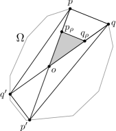
Figure 1. The area of the triangle $(op_{\rho},q_{\rho})$ is bounded by $C\rho^{2}$.

Then the volume of the triangle $(op_{\rho}q_{\rho})$ with respect to the Hilbert geometry of $\Omega$ is less than or equal to its volume with respect to the Hilbert geometry of the quadrilateral $(pqp^{\prime}q^{\prime})$. However, the distances of $p_{\rho}$ and $q_{\rho}$ from $o$ remain the same in both Hilbert geometries.

Up to a change of chart, we can suppose that this quadrilateral is actually a square. This allows us to use Theorem 1 from [Ver11] which states that the Hilbert geometry of the square is bi-lipschitz to the product of the Hilbert geometries of its sides, using the identity as a map. In other words it is bi-lipschitz to the Euclidean plane, with a lipschitz constant equal to $C_{0}>1$, independent of our initial conditions.

Therefore our affine triangle is inside a Euclidean disc of radius $C_{0}\rho$, which implies that its area with respect to the Hilbert geometry of $\Omega$ is less than $C_{0}^{4}\times\pi\times\rho^{2}$. ∎

To prove that the volume entropy is bounded from below by the approximabilty we will need to bound from below the length of certain segments in a given Hilbert geometry $\Omega$. To do so will compare their length in the initial convex with their length in a convex projectively equivalent to a triangle, and containing the initial convex $\Omega$.

Let us make this precise. Consider four points $a$, $b$, $c$ and $d$ in the Euclidean plane $({\mathbb{R}}^{2},\langle\cdot\rangle)$ such that $\mathcal{Q}=(abcd)$ is a convex quadrilateral. We assume that the scalar products $\langle\vec{ab},\vec{bc}\rangle$ and $\langle\vec{bc},\vec{cd}\rangle$ are positive and we let $q$ be the intersection point between the straight lines $(ab)$ and $(cd)$.

Suppose that $\Omega$ is a convex domain such that the segments $[a,b]$, $[b,c]$ and $[c,d]$ belong to its boundary.

Given $p$ a point in the convex domain $\Omega$ we denote by $p^{\prime}$ the intersection between the straight line $(pq)$ and the segment $[b,c]$, and we define $s={bp^{\prime}}/{bc}.$

We then denote by $[b(r),c(r)]$ the image of the segment $[b,c]$ under the dilation centred at $p$ with ratio $0<\tanh(r)<1$. The image of the segment $[b,c]$ under the dilation centred at $q$ sending $p^{\prime}$ on $p$ will be denoted by $[B,C]$.

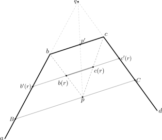
Figure 2. Distance estimate of Claim 10

Claim 10.

The following inequality is satisfied under the above assumption:

(16) $$\begin{split}d_{\Omega}\bigl{(}b(r),c(r)\bigr{)}\geq\frac{1}{2}\ln\biggl{(}\frac{bc}{s\cdot BC}&\frac{\tanh(r)}{1-\tanh(r)}+1\biggr{)}\\ &+\frac{1}{2}\ln\biggl{(}\frac{bc}{(1-s)\cdot BC}\frac{\tanh(r)}{1-\tanh(r)}+1\biggr{)}\text{.}\end{split}$$

Proof.

Straightforward computation, using the fact that the convex domain $\Omega$ is inside the convex $Q$ obtained as the intersection of the half planes defined by the lines $(ab)$, $(bc)$ and $(cd)$, and therefore

$$d_{\Omega}\bigl{(}b(r0,c(r)\bigr{)}\geq d_{Q}\bigl{(}b(r),c(r)\bigr{)}.$$

Let $b^{\prime}(r)$ be the intersection of the lines $(ab)$ and $\bigl{(}b(r)c(r)\bigr{)}$, and let $c^{\prime}(r)$ be the intersection of the lines $(cd)$ and $\bigl{(}b(r)c(r)\bigr{)}$. Then we have

$$d_{Q}\bigl{(}b(r0,c(r)\bigr{)}=\frac{1}{2}\ln\biggl{(}\frac{b(r)c^{\prime}(r)}{c(r)c^{\prime}(r)}\cdot\frac{c(r)b^{\prime}(r)}{b(r)b^{\prime}(r)}\biggr{)}.$$

Let us focus on the first ratio. On the one hand $b(r)c^{\prime}(r)=b(r)c(r)+c(r)c^{\prime}(r)$, and on the second hand following Thales’s theorem

(17) $$\begin{split}&b(r)c(r)=\tanh(r)bc\\ &c(r)c^{\prime}(r)=(1-\tanh(r))pC.\end{split}$$

But $pC=BC\cdot(p^{\prime}c/bc)=(1-s)BC$, and therefore we obtain

$$\ln\biggl{(}\frac{b(r)c^{\prime}(r)}{c(r)c^{\prime}(r)}\biggr{)}=\ln\biggl{(}\frac{bc}{(1-s)\cdot BC}\frac{\tanh(r)}{1-\tanh(r)}+1\biggr{)}.$$

The second ratio is treated in the same way. ∎

1.4. Intrinsic and extrinsic Hausdorff topologies of Hilbert Geometries

We describe the link between the Hausdorff topology induced by an Euclidean metric with the Hausdorff topology induced by the Hilbert metric on compact subset of an open convex set.

We recall that the Lowner ellipsoid of a compact set, is the ellipsoid with least volume containing that set. In this section we will suppose, without loss of generality, that $\Omega$ is a bounded open convex set, whose Lowner ellipsoid $\mathcal{E}$ is the Euclidean unit ball and $o$ is the center of that ball. It is a standard result that $(1/n)\mathcal{E}$ is then contained in $\Omega$, i.e., we have the following sequence of inclusions

(18) $$\frac{1}{n}\mathcal{E}\subset\Omega\subset\mathcal{E}$$

Definition 11 (Asymptotic ball and sphere).

We call asymptotic ball of radius $R$ centred at $o$ the image of $\Omega$ by the dilation of ratio $\tanh R$ centred at $o$, and we denote it by $AsB(o,R)$. The image of the boundary $\partial\Omega$ by the same dilation will be called the asymptotic sphere of radius $R$ centred at $o$ and denoted by $AsS(o,R)$.

Recall that the Hausdorff distance is a distance between non empty compact subsets in a metric space. We shall use both the Euclidean and Hilbert distance and we will use the terminology Hausdorff-Euclidean and Hausdorff-Hilbert to distinguish both cases.

We would like to relate the Hausdorff-Hilbert neighbourhoods of the asymptotic ball $AsB(o,R)$ with its Hausdorff-Euclidean neighbourhoods.

Proposition 12.

Let $\Omega$ be a convex domain and let $o$ be the centre of its Lowner ellipsoid, which is supposed to be the unit Euclidean ball.

1. The $(1-\tanh(R))/2n$-Hausdorff-Euclidean neighborhood of the asymptotic ball $AsB(o,R)$ is contained in its $\bigl{(}(\ln 3)/2\bigr{)}$-Hausdorff-Hilbert neighborhood.

2. For any $K>0$, the $K$-Hausdorff-Hilbert neighborhood of the asymptotic ball $AsB(o,R)$ is contained in its $\bigl{(}1-\tanh(R)\bigr{)}$-Hausdorff-Euclidean neighborhood.

Proof.

For any point $p\in\partial\Omega$ on the boundary of $\Omega$, and for $0<t<1$ let $\varphi_{t}(p)=o+t\cdot\overrightarrow{op}$. This map sends $\partial\Omega$ bijectively on the asymptotic sphere $AsS(o,\operatorname{arctanh}t)$ centred at $o$ with radius $\operatorname{arctanh}t$.

Proof of part (i) of the Proposition:

Any point of a compact set in the $(1-\tanh(R))/2n$-Hausdorff-Euclidean neighborhood of $AsB(o,R)$, either lies inside $AsB(o,R)$, or is contained in an Euclidean ball of radius $(1-\tanh(R))/2n$ centred on a point of $AsB(o,R)$.

We recall that the ball of radius $1/n$ is a subset of $\Omega$, and thus so is the ball of radius $1/2n$, that is

$$\frac{1}{2n}\mathcal{E}\subset\frac{1}{n}\mathcal{E}\subset\Omega\text{.}$$

Let $p\in\partial\Omega$ be a point on the boundary. By convexity, the interior of $K(p)$ the convex hull of $p$ and $1/n\mathcal{E}$ is a subset of $\Omega$ — it is the projection of a cone of basis $1/n\mathcal{E}$. Hence $\mathcal{E}_{p,\alpha}$, the image of $1/n\mathcal{E}$ by the dilation of ratio $0<\alpha<1$ centred at $p$, lies in the ”cone” $K(p)$. The set $\mathcal{E}_{p,\alpha}$ is therefore an Euclidean ball of radius $\alpha/n$ centred at $\varphi_{1-\alpha}(p)$, and it is a subset of $\Omega$.

A point in the Euclidean ball of radius $\alpha/2n$ centred at $\varphi_{1-\alpha}(p)$ is at a distance less or equal to $1/2\ln 3$ from $\varphi_{1-\alpha}(p)$ with respect to the Hilbert distance of $\mathcal{E}_{p,\alpha}$.

Now a standard comparison arguments states that for any two points $x$ and $y$ in $\mathcal{E}_{p,\alpha}\subset\Omega$ the following inequality occurs

$$d_{\Omega}(x,y)\leq d_{\mathcal{E}_{p,\alpha}}(x,y)\text{.}$$

From this inequality it follows that any point in the Euclidean ball of radius $\alpha/2n$ centred at $\varphi_{1-\alpha}(p)$ is in the Hilbert metric ball centred at $\varphi_{1-\alpha}(p)$ of radius $1/2\ln 3$.

Now for any $1\geq\alpha>1-\tanh R$, the Euclidean ball of radius $\alpha/2n$ contains the Euclidean ball of radius $(1-\tanh R)/2n$.

This implies that for any point $x$ in the asymptotic ball $AsB(o,R)$, the Euclidean ball of radius $(1-\tanh R)/2n$ centred at $x$ is contained in the Hilbert ball of radius $1/2\ln 3$ centred at the $x$, which allows us to obtain the first part of our claim.

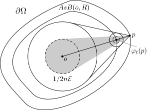
Figure 3. Illustration of Proposition 12’s proof

Proof of part (ii) of the Proposition: This follows from the fact that under our assumptions, $\Omega$ itself is in the $(1-\tanh R)$ Hausdorff-Euclidean neighborhood of the asymptotic ball $AsB(o,R)$. ∎

Corollary 13.

Let $\Omega$ be a convex domain and let $o$ be the centre of its Lowner ellipsoid, which is supposed to be the unit Euclidean ball.

1. The $(1-\tanh(R+\ln 2))/2n$-Hausdorff-Euclidean neighborhood of $B(o,R)$ is contained in its $\ln\bigl{(}3(n+1)\bigr{)}$-Hausdorff-Hilbert neighborhood.

2. For any $K>0$, the $K$-Hausdorff-Hilbert neighborhood of $B(o,R)$ is contained in its $\Bigl{(}1-\tanh\bigl{(}R+K-\ln(n+1)\bigr{)}\Bigr{)}$-Hausdorff-Euclidean neighborhood.

The proof of this corrollary is a straightforward consequence of the following lemma applied to the conclusion of the Proposition 12.

Lemma 14.

Let $\Omega$ be a convex domain, and suppose that $o$ is a point in the interior of $\Omega$ such that the unit Euclidean open ball centred at $o$ contains $\Omega$, and $\Omega$ contains the Euclidean closed ball centred at $o$ of radius $1/(2n)$. Then we have

(19) $$\begin{split}B(o,R)\subset AsB(o,R+\ln 2)\text{, and}\\ AsB(o,R)\subset B\bigl{(}o,R+\ln(n+1)\bigr{)}.\end{split}$$

This lemma is a refinement of a result of [CV04] in our case.

Proof of Lemma 14.

Let $x$ be a point on the boundary $\partial\Omega$ of $\Omega$, and let $x^{*}$ be the second intersection of the straight line $(ox)$ with $\partial\Omega$. Then our assumption implies the next two inequalities.

(20) $$\begin{split}1/2n<xo\leq 1\\ 1/2n<ox^{*}\leq 1\end{split}$$

Actually the first inclusion is always true. Indeed suppose $y$ is on the half line $[ox)$ such that $d_{\Omega}(o,y)\leq R$ which in other words implies that we have

$$\frac{ox}{yx}\frac{yx^{*}}{ox^{*}}\leq e^{2R}$$

therefore

$$ox\leq e^{2R}\frac{ox^{*}}{yx^{*}}(ox-oy)\leq e^{2R}(ox-oy)$$

which implies in turn that

$$oy\leq\frac{e^{2R}-1}{e^{2R}}ox\leq\bigl{(}1-e^{-2R}\bigr{)}ox\leq\tanh(R+\ln 2)ox\text{.}$$

Now regarding the second inclusion: consider $y$ a point on the half line $[ox)$ such that $oy\leq\tanh(R)ox$. On the one hand we have

$$\frac{ox}{yx}=\frac{ox}{ox-oy}\leq\frac{1}{1-\tanh(R)}=\frac{e^{2R}+1}{2}\text{.}$$

and, on the other hand thanks to the inequalities (20) we get

(21) $$\frac{yx^{*}}{ox^{*}}\leq\frac{ox+ox^{*}}{ox^{*}}\leq 1+\frac{ox}{ox^{*}}\leq 1+2n\text{,}$$

which implies that

(22) $$\frac{ox}{yx}\frac{yx^{*}}{ox^{*}}\leq\frac{e^{2R}+1}{2}(1+2n)\leq(1+2n)e^{2R}\leq(1+n)^{2}e^{2R}\text{.}$$

The conclusion follows. ∎

1.5. Distance function to a sphere in a Hilbert geometry

This section is an adaptation in the realm of Hilbert geometries of a result concerning the spheres in a Minkowski space provided to the author by A. Thompson [Tom].

Let us first start by recalling the following important fact regarding the distance of a point to a geodesic in a Hilbert geometry (see Busemann [Bus55], chapter II, section 18, page 109):

Proposition 15.

Let $(\Omega,d_{\Omega})$ be a Hilbert Geometry. The distance function of a straight geodesic (that is given by an affine line) to a point is a peakless function, i.e., if $\gamma\colon[t_{1},t_{2}]\to\Omega$ is a geodesic segment, then for any $x\in\Omega$ and $t_{1}\leq s\leq t_{2}$ one has

$$d_{\Omega}\bigl{(}x,\gamma(s)\bigr{)}\leq\max\biggl{\{}d_{\Omega}\bigl{(}x,\gamma(t_{1})\bigr{)},d_{\Omega}\bigl{(}x,\gamma(t_{2})\bigr{)}\biggr{\}}\text{.}$$

Let us now turn our attention to metric spheres in a two dimensional Hilbert geometry.

Proposition 16.

Let $(\Omega,d_{\Omega})$ be a two dimensional Hilbert Geometry. Suppose $o$ is a point of $\Omega$, and $p$ and $q$ are two points on the intersection of the metric sphere $S(o,R)$ centred at $o$ and radius $R$ with a line passing by $o$. If $C$ denotes one of the arcs of the sphere $S(o,R)$ from $p$ to $q$, then for any point $p^{\prime}$ on the half line $[o,p)$, the function $\varphi(x)=d_{\Omega}(p^{\prime},x)$ is monotonic on $C$.

Proof.

Let $p,x,y,q$ be points on that order on $C$. We have to show that

$$d_{\Omega}(p^{\prime},x)\leq d_{\Omega}(p^{\prime},y)\text{.}$$

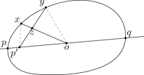
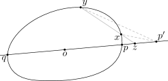
Figure 4. Monotonicity of the distance of a point to a sphere

Suppose first that that the line segments $[o,x]$ and $[p^{\prime},y]$ intersects at a point $z$. Hence we have

$$d_{\Omega}(o,x)+d_{\Omega}(p^{\prime},y) = \bigl{(}d_{\Omega}(o,z)+d_{\Omega}(z,x)\bigr{)}+\bigl{(}d_{\Omega}(p^{\prime},z)+d_{\Omega}(z,y)\bigr{)}$$

$$= \bigl{(}d_{\Omega}(p^{\prime},z)+d_{\Omega}(z,x)\bigr{)}+\bigl{(}d_{\Omega}(o,z)+d_{\Omega}(z,y)\bigr{)}$$

$$\geq d_{\Omega}(p^{\prime},x)+d_{\Omega}(o,y)\text{.}$$

now, as $d_{\Omega}(o,y)=d_{\Omega}(o,x)=R$, the result follows.

Suppose now that $[o,x]$ and $[p^{\prime},y]$ do not intersect, which implies that $p^{\prime}$ is outside the ball $B(o,R)$. Then the line $(yx)$ intersects $(op)$ at $z$. Because $x$ and $y$ lie on the sphere of radius $R$, $d_{\Omega}(o,z)>R$. Also, as $p$ is one of the nearest points to $p^{\prime}$ on $C$, we have $d_{\Omega}(p^{\prime},z)\leq d_{\Omega}(p^{\prime},p)\leq d_{\Omega}(p^{\prime},y)$ Hence if apply the proposition 15 to the segment $[z,y]$ and $p^{\prime}$, as $x\in[z,y]$ we get

$$d_{\Omega}(p^{\prime},x)\leq\max\bigl{\{}d_{\Omega}(p^{\prime},z),d_{\Omega}(p^{\prime},y)\bigr{\}}=d_{\Omega}(p^{\prime},y).$$

∎

2. Volume entropy and approximability

This section is devoted to the proof of the main theorem. This is done in two steps. The first step consists in bounding the entropy from above in dimension 2 and 3 by the approximability thanks to the study of the volume growth in polytopes. The second step is to bound from below the entropy. This is done by exhibiting a separated subset of the Hilbert geometry whose growth is bigger than the approximability. We conclude this section with the various corollaries implied.

Theorem 17.

Let $\Omega$ be a bounded convex domain in ${\mathbb{R}}^{2}$ or ${\mathbb{R}}^{3}$. The double of the approximabilities of $\Omega$ are bigger than the volume entropies, i.e.,

$$\operatorname{\underline{Ent}}(\Omega)\leq 2\underline{a}(\Omega)\text{, and }\operatorname{\overline{Ent}}(\Omega)\leq 2\overline{a}(\Omega)\text{.}$$

The proof of this theorem relies on the following stronger statement which is a sort of uniform bound on the volume of metric balls and metric spheres in a polytopal Hilbert geometry. The key fact is that this bound depends, in a coarse sense, linearly on the number of verticies of the polytope.

Theorem 18.

Let $n=2$ or $n=3$. There are affine maps $a_{n},b_{n}$ from ${\mathbb{R}}\to{\mathbb{R}}$ and polynomials $q_{n},p_{n-1}$ of degree $n$ and $n-1$ such that for any open convex polytope ${\mathcal{P}}_{N}$ with $N$ vertices inside the unit Euclidean ball of ${\mathbb{R}}^{n}$ and containing the ball of radius $1/2n$, one has

(23) $$\begin{array}[]{rcl}{\rm Vol}_{n-1,{\mathcal{P}}_{N}}S_{{\mathcal{P}}_{N}}(o,R)&\leq&a_{n}(N)p_{n-1}(R)\\ {\rm Vol}_{{\mathcal{P}}_{N}}B_{{\mathcal{P}}_{N}}(o,R)&\leq&b_{n}(N)q_{n}(R)\text{.}\end{array}$$

The same result holds for the asymptotic balls.

Let us stress out that our method also yields a control in terms of the vertices in higher dimension as well, using the so called upper bound conjecture proved by McMullen [McM71, MS71], but alas a polynomial of degree strictly bigger than $1$ replaces the affine functions $a_{n}$ and $b_{n}$. This is why we can’t state the equality in the Main Theorem in higher dimensions.

Notice that this theorem is still valid if we replace the Hausdorff measures by any measures defined by a pair of proper densities $f\in\mathcal{PD}_{n}$ and $g\in\mathcal{PD}_{n-1}$. The change of measures will only impact the values of the constants.

Proof of theorem 18.

We will have to deal with the dimension two and the dimension three separately, even if both cases follow the same main steps.

The first step of our proof consists in proving the first inequality of (23) for the Holmes-Thompson measure and for an asymptotic sphere. The uniform inclusion of metric balls into asymptotic balls (19) imply then the result for the metric spheres thanks to the monotonicity of the Holmes-Thompson measure lemma 6.

The second step is an integration using the co-area inequality (25), wich allows us to get the second inequality of (23) for metric balls with respect to the Buseman measure.

Let us now make all this more precise. We fix a Polytope ${\mathcal{P}}_{N}$ with $N$ verticies and for any real $R>0$ we let $P_{R}$ be the asymptotic ball of radius $R$ centred at $o$, and let $\partial P_{R}$ be the associated asymptotic sphere. We also introduce the constant $c_{n}=\ln(n+1)$.

Two dimensional case: The idea is to found an upper bound on the length of each eadge of the asymptotic sphere $\partial P_{R}$, depending only on $R$.

To do so, we can use the fact that eadge edge belongs to the triangle defined by joining its extremities to the point $o$. Hence, thanks to the triangular inequality its length is less than the sum of these two other segments. However, using the second inclusion (19) of lemma 14, we know that the asymptotic ball $P_{R}$ is inside the Hilbert ball of radius $R+c_{2}$ centred at $o$ of the convex polygon $\mathcal{P}_{N}$. Hence the length of each edge is less than $2\cdot(R+c_{2})$. Therefore the length of the polygon $\partial P_{R}$ is less than $N\cdot 2\cdot(R+c_{2})$.

Following the first inclusion (19) of Lemma 14, the metric ball of radius $r$ centred at $o$ is a subset of the asymptotic ball of radius $r+\ln 2$ centred at $o$. Therefore, we can use the monotonicity of the Holmes-Thompson length (see Lemma 6) to get for all $r>0$,

(24) $$\text{length}_{\mathcal{P}_{N}}(S_{\mathcal{P}_{N}}(o,r))\leq\text{length}_{\mathcal{P}_{N}}(\partial P_{r+\ln(2)})\leq N\cdot 2(r+\ln 2+c_{2})\text{.}$$

Now using the co-area inequality of Lemma 8, taking into account that the Busemann length is equal to the Holmes-Thompson length one gets

(25) $$\frac{\partial}{\partial r}{\rm Vol}_{\mathcal{P}_{N}}(B_{\mathcal{P}_{N}}(o,r))\leq\frac{\pi}{4}\cdot N\cdot 2(r+\ln 2+c_{2})\text{.}$$

Hence, integrating the inequality (25) over the interval $[0,R]$, we finally obtain the following inequality for the ball of radius $R>0$

(26) $${\rm Vol}_{\mathcal{P}_{N}}(B_{\mathcal{P}_{N}}(o,R))\leq\frac{\pi}{4}\cdot N\cdot(R^{2}+2(\ln 2+c_{2})R)\text{.}$$

The inequalities (24) and (26) are the expected results in dimension two.

Three dimensional case: Once again the idea is to found an upper bound on the area of faces of the asymptotic sphere $\partial P_{R}$. Alas, contrary to the two dimensional cases, there is not a unique type of faces, and is therefore pointless to look for an upper bound depending only on the radius $R$.

However, each face can be seen as the basis of a pyramid with apex the point $o$. All other faces are then triangles, whose areas can be bounded thanks to the lemma  9. The analog of the triangle inequality is available in the form of the minimality of the Holmes-Thompson area (see Berck [Ber09]). In other words, the Holmes-Thompson area of each face of $\partial P_{R}$ is less than the sum of the Holmes-Thompson areas of the triangles obtained as the convex hull of $o$ and an edge of the given face of $\partial P_{R}$. Let us call $\mathcal{T}_{o}$ such a triangle (the subscript $o$ is to stress the fact that the point $o$ is one of its verticies)

To bound the area of the triangle $\mathcal{T}_{o}$ it suffices to focus on the intersection of the polytope ${\mathcal{P}}_{N}$ with the affine plane containing the triangle $\mathcal{T}_{o}$. This is a polygon $\tilde{P}$, to which we can apply the Lemma 9 which bounds from above the area of a two dimensional triangles inside a metric ball centred on one of its vertex. Which is exactly the situation of our triangle $\mathcal{T}_{o}$ with respect to the Hilbert geometry associated to the polygon $\tilde{P}$. Indeed it is included in the asymptotic ball of radius $R$, and again thanks to lemma 14 we know that it is inside the metric ball of radius $R+c_{3}$ with respect to Hilbert geometry of $\mathcal{P}_{N}\in{\mathbb{R}}^{3}$. As $\tilde{P}$ is a plane section of $\mathcal{P}_{N}\in{\mathbb{R}}^{3}$, this still holds for $\mathcal{T}_{o}$ seen as a subset of $\tilde{P}$. Hence Lemma 9 implies that the area of the triangle $\mathcal{T}_{o}$ is less than $C(R+c_{3})^{2}$, for some constant $C>1$ independent of $R$.

Therefore, if $e(N)$ is the number of edges of $\mathcal{P}_{N}$, the area of the asymptotic sphere $\partial P_{R}$ is less than $2e(N)C(R+c_{3})^{2}$.

Let $f(N)$ be the number of faces of $\mathcal{P}_{N}$ and let us recall Euler’s formula:

$$N-e(N)+f(N)=2\text{.}$$

Each face being surrounded by at least three edges and each edge belonging to two faces, one has the classical inequality (where equality is obtained in a simplex),

$$3f(N)\leq 2e(N)\text{.}$$

Combining the previous two inequalities we get a linear upper bound of the number of edges by the number of vertexes as follows:

$$2\leq N-(1/3)e(N)\Rightarrow e(N)\leq 3N-6\text{.}$$

Hence the area of of the asymptotic sphere $\partial P_{R}$ is less than $(3N-6)\cdot 2C\cdot(R+c_{3})^{2}$.

We can now conclude almost as in the two dimensional case. Following the first inclusion (19) of Lemma 14, the metric ball of radius $r$ centred at $o$ is a subset of the asymptotic ball of radius $r+\ln 2$ centred at $o$. Therefore, we can use the monotonicity of the Holmes-Thompson area measure (see Lemma 6) to get for all $r>0$,

(27) $${\rm Vol}_{2,\mathcal{P}_{N}}(S_{\mathcal{P}_{N}}(o,r))\leq{\rm Vol}_{2,\mathcal{P}_{N}}(\partial P_{r+\ln 2})\leq(3N-6)2C(r+\ln 2+c_{3})^{2}\text{.}$$

Notice that this inequality (27) corresponds to the first part of the inequality (23).

The rough monotonicity of the Busemann measure (see the right hand side of the inequality (15) in Lemma 7) states that the Busemann area is smaller that the Holmes-Thompson one, hence combined with the inequality (27) above, we get that for all $r>0$

(28) $$\operatorname{Area}_{\mathcal{P}_{N}}(S_{\mathcal{P}_{N}}(o,r))\leq(3N-6)\cdot 2C\cdot(r+\ln 2+c_{3})^{2}\text{.}$$

Taking into account the co-area inequality (see Lemma 8) in conjunction with the inquality (28) leads to the following differential inequality

(29) $$\frac{\partial}{\partial r}{\rm Vol}_{\mathcal{P}_{N}}(B_{\mathcal{P}_{N}}(o,r))\leq 2\cdot(3N-6)\cdot 2C\cdot(r+\ln 2+c_{3})^{2}\text{,}$$

which we can integrate over the interval $[0,R]$ to finally obtain that for all $R>0$

(30) $${\rm Vol}_{\mathcal{P}_{N}}(B_{\mathcal{P}_{N}}(o,R))\leq 2\cdot(N-2)\cdot 2C\cdot\bigl{(}(r+\ln 2+c_{3})^{3}-c_{3}^{3}\bigr{)}\text{.}$$

This concludes our proof in the three dimensional case. ∎

Le us remark that if we link this to our study of the asymptotic volume of the Hilbert geometry of polytopes [Ver13] we obtain the following corollary

Corollary 19.

Let ${\mathcal{P}}_{N}$ be an open convex polytope with $N$ vertices in ${\mathbb{R}}^{n}$, for $n=2$ or $3$, then there are three constants $\alpha_{n}$, $\beta_{n}$ and $\gamma_{n}$ such that for any point $p\in{\mathcal{P}}_{N}$ one has

$$\alpha_{n}\cdot N\leq\liminf_{R\to+\infty}\frac{{\rm Vol}_{\mathcal{P}_{N}}B_{{\mathcal{P}}_{N}}(p,R)}{R^{n}}\leq\beta_{n}\cdot N+\gamma_{n}$$

Now let us come back to our initial problem and see how theorem 18 implies theorem 17.

Proof of theorem 17 .

We remind the reader that ${\rm Vol}_{n-1,\Omega}$ stands for the $n-1$-dimensional Holmes-Thompson measure. Let $o$ be the centre of the Lowner ellipsoid of $\Omega$ which is supposed to be the unit Euclidean ball. We consider $R$ large enough in order to have the Euclidean ball of radius $1/2n$ inside all the asymptotic balls involved in the sequel.

The idea of the proof consists in replacing for all $R$ large enough the convex set $\Omega$ by a convex polytope $\mathcal{P}_{R}$ such that

• $\mathcal{P}_{R}$ is a subset of $\Omega$;

• The asymptotic ball $P_{R}$ of the polytope $\mathcal{P}_{R}$ is inside the $\bigl{(}1-\tanh(R)\bigr{)}/2n$-Euclidean neighborhood of the corresponding asymptotic ball $AsB_{\Omega}(o,R)$ of $\Omega$.

• the exponential volume growth, with respect to the geometry of $\Omega$, of the two families of asymptotic balls $(P_{R})_{R\in{\mathbb{R}}}$ and $(AsB_{\Omega}(o,R))_{R\in{\mathbb{R}}}$ are the same.

Let us insist on the fact that the convex polytope $\mathcal{P}_{R}$ depends on $R$.

Then using Theorem 18 we will bound from above the area in dimension three or the perimeter in dimension two of the convex polytope $P_{R}$ by a function depending linearly on the number of verticies of $P_{R}$ and polynomialy on $R$. This will allow us to conclude.

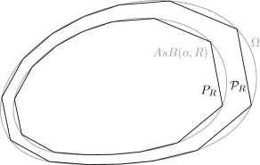
Figure 5. The asymptotic ball and an approximating polytope

Fix $R$. Among all polytopes included both in the asymptotic ball $AsB_{\Omega}(o,R)$ and its $\bigl{(}1-\tanh(R)\bigr{)}/2n$ Euclidean-Hausdorff neighborhood pick a polytope $P_{R}$ with the minimal number of verticies $N(R)$. Notice that we have

(31) $$N(R)=N\biggl{(}\frac{1-\tanh(R)}{2n\tanh(R)},\Omega\biggr{)}\text{.}$$

Claim: There exists a constant $C>0$ such that for all $R$ the following inclusions occur

(32) $$AsB_{\Omega}\bigl{(}o,R-C\bigr{)}\subset P_{R}\subset AsB_{\Omega}(o,R)\text{.}$$

To prove this claim, on the one hand we deduce from the first inclusion of Lemma 14 that

$$B_{\Omega}(o,R-\ln 2)\subset AsB_{\Omega}(o,R)\text{.}$$

On the other hand the comparison of both Hilbert and Euclidean-Hausdorff neighborhoods, as stated in Proposition 12, implies that the convex polytope $P_{R}$ lies in the $(\ln 3)/2$-Hilbert-Hausdorff neighborhood of the asymptotic ball $AsB_{\Omega}(o,R)$. From these we deduce the inclusion

(33) $$B_{\Omega}\bigl{(}o,R-\ln 6\bigr{)}\subset P_{R}\subset AsB_{\Omega}(o,R)\text{.}$$

Taking into account the second inclusion of Lemma 14 we finaly get

(34) $$AsB_{\Omega}\bigl{(}o,R-\ln 6-\ln(n+1)\bigr{)}\subset P_{R}\subset AsB_{\Omega}(o,R)\text{,}$$

which proves our claim with $C=\ln 6+\ln(n+1)$.

Thanks to the monotonicity of the Holmes-Thompson measure (see Lemma 6) we know that the area of the boundary $\partial P_{R}$ is less than the area of the asymptotic sphere $AsS_{\Omega}(o,R)$, but larger than the area of the asymptotic sphere of radius $R-C$, that is:

(35) $${\rm Vol}_{n-1,\Omega}\bigl{(}AsS_{\Omega}(o,R-C)\bigr{)}\leq{\rm Vol}_{n-1,\Omega}(\partial P_{R})\leq{\rm Vol}_{n-1,\Omega}\bigl{(}AsS_{\Omega}(o,R)\bigr{)}\text{.}$$

From the equation (35) we deduce that the logarithms of the areas of $\partial P_{R}$ and $AsS_{\Omega}(o,R)$ are asymptotically the same in the following sense

(36) $$\lim_{R\to+\infty}\dfrac{\ln{\rm Vol}_{n-1,\Omega}\bigl{(}AsS_{\Omega}(o,R)\bigr{)}}{\ln{\rm Vol}_{n-1,\Omega}(\partial P_{R})}=1\text{.}$$

Let us denote by ${\mathcal{P}}_{R}$ the image of $P_{R}$ by the dilation of ratio $1/(\tanh R)$. This is the dilation sending $AsB_{\Omega}(o,R)$ to $\Omega$. Hence, by construction, ${\mathcal{P}}_{R}\subset\Omega$ and therefore we have

(37) $${\rm Vol}_{n-1,\Omega}(\partial P_{R})\leq{\rm Vol}_{n-1,{\mathcal{P}}_{R}}(\partial P_{R})\text{.}$$

Now thanks to Theorem 18, for $n=2$ or $n=3$ and $R>0$ such that $\tanh(R)>3/4$, there are two constants $a_{n}$, $b_{n}$ and a polynomial $Q_{n}$ of degree $n$ such that

(38) $${\rm Vol}_{n-1,\Omega}(\partial P_{R})\leq(a_{n}N(R)+b_{n})Q_{n}(R)\text{.}$$

To conclude remark that

$$\liminf_{R\to+\infty}\frac{\ln(N(R))}{R}=2\underline{a}(\Omega)\text{, and }\limsup_{R\to+\infty}\frac{\ln(N(R))}{R}=2\overline{a}(\Omega)\text{,}$$

and use it with the inequality (38) to get for instance

$$\limsup_{R\to+\infty}\dfrac{\ln{\rm Vol}_{n-1,\Omega}(\partial P_{R})}{R}\leq 2\overline{a}(\Omega).$$

Finally the limit (36) implies that

$$\limsup_{R\to+\infty}\dfrac{\ln{\rm Vol}_{n-1,\Omega}\bigl{(}AsS_{\Omega}(o,R)\bigr{)}}{R}\leq 2\overline{a}(\Omega).$$

The left hand sides of this last inequality is easily seen to be the spherical entropy (see (13)), which ends our proof. ∎

The following corollary follows from Brons̆teĭn and Ivanov’s Theorem 31 which states that $2\overline{a}\leq n-1$.

Corollary 20.

Let $\Omega$ be an open bounded convex set in ${\mathbb{R}}^{n}$, for $n=2$ or $3$, then

$$\operatorname{\overline{Ent}}(\Omega)\leq n-1\text{.}$$

We are now going to study the reverse inequality.

Theorem 21.

Let $\Omega$ be an bounded convex domain in ${\mathbb{R}}^{n}$. The volume entropies of $\Omega$ are bigger or equal to twice the approximabilities of $\Omega$, i.e.,

$$2\underline{a}(\Omega)\leq\operatorname{\underline{Ent}}(\Omega)\text{ and }2\overline{a}(\Omega)\leq\operatorname{\overline{Ent}}(\Omega)\text{.}$$

Proof of Theorem 21.

Without loss of generality we suppose that the Euclidean unit ball is the Lowner ellipsoid of $\Omega$, and $o$ is the centre of that ball.

The idea of the proof is the following:

• We will show that for a good positive $\delta$ and any positive real number $R$ there exists a $\delta$-separated set $\mathcal{S}_{R}$ in the metric ball of radius $B(o,R+2\delta)$, such that the convex closure $P_{R}$ of that set contains the ball $B(o,R)$.

• We will then use the fact that the cardinal of this $\delta$-separated set will be larger than the cardinal of the set of verticies of a vertex minimising convex polytope included in the annulus $B(o,R+2\delta)\setminus B(o,R)$.

  In other words, the number of points in the $\delta$-separated will be bounded from below by the number $N\bigl{(}\varepsilon(R),\Omega\bigr{)}$ from the introduction. Here $\varepsilon$ will be a function of $R$.

• To conclude we will take into account that the union of the open metric balls of radius $\delta/2$ centred at the point of the $\delta$-separated set $\mathcal{S}_{R}$ are disjoints and are in the ball $B(o,R+3\delta)$. Thus getting a lower bound on the volume of the ball $B(o,R+3\delta)$ in terms of $N\bigl{(}\varepsilon(R),\Omega\bigr{)}$ times a constant depending on the dimension.

Let us now start the proof. Consider the $(\ln 3)/2$-Hilbert neighborhood of the metric ball $B(o,R)$, that is

$$V(R)=B(o,R+(\ln 3)/2)\text{,}$$

and take a maximal $\delta=(\ln 3)/4$-separated set $\mathcal{S}_{R}$ on its boundary. This set contains $\#\mathcal{S}_{R}$ points.

Now let us take the convex hull $\mathcal{C}_{R}$ of these points. This is a polytope with $N_{2}(R)\leq\#\mathcal{S}_{R}$ vertices.

Claim 22.

The polytope $\mathcal{C}_{R}$ is included in the $2\delta$-Hilbert neighborhood of $B(o,R)$ and contains $B(o,R)$.

Notice that if the claim holds, then for some real constant $c$ independent of $R$ (see corollary 13 once again), we have

(39) $$\#\mathcal{S}_{R}\geq N_{2}(R)\geq\widetilde{N}(R-c):=N\bigl{(}1-\tanh(R-c)/4,AsB(o,R-c)\bigr{)}.$$

Proof of claim 22.

First notice that $V(R)$ is a convex set (see Busemann [Bus55], chapter II, section 18, page 105). Therefore the convex hull is inside the $2\delta$-Hilbert neighborhood of $B(o,R)$, that is $V(R)$.

Now let us suppose by contradiction that $\mathcal{C}_{R}$ does not contain $B(o,R)$. Hence there exists some points $q$ in $B(o,R)$ which is not in $\mathcal{C}_{R}$.

We will show that we can find a point on the sphere $S(o,R+2\delta)$ which is at a distance bigger that $\delta$ from all points of $\mathcal{S}_{R}$, which will contradict its maximality.

Under our assumption, the Hahn-Banach separation theorem asserts that there exists a linear form $a$, some constant $c$ and a hyperplane $H=\{x\mid a(x)=c\}$ which separates $q$ and $\mathcal{C}_{R}$, i.e., $a(q)>c$ and $a(x)<c$ for all $x\in\mathcal{C}_{R}$. Consider then $H_{q}=\{x\mid a(x)=a(q)\}$ the parallel hyperplane to $H$ containing $q$. Let us say that a point $x$ such that $a(x)\geq a(q)$ is above the hyperplane $H_{q}$.

Then let us define by $V_{o}^{\prime}=\{x\in\partial V(R)\mid a(x)\geq a(q)\}$ the part of the boundary of $V(R)$ which is above $H_{q}$.

Now we want to metrically project each point of $V_{o}^{\prime}$ onto $H_{q}$, that is to say that to each point of $V_{o}^{\prime}$ we associate its closest point on $H_{q}$.

However if $\Omega$ is not strictly convex, the projection might not be unique (see the appendix A), that is why we are going to distinguish two cases.

First case: The convex set $\Omega$ is strictly convex, then the metric projection is a map from $V_{o}^{\prime}$ to $H_{q}$ and it is continuous, furthermore the point on $H_{q}\cap V_{o}^{\prime}$ are fixed and by convexity $H_{q}\cap V_{o}^{\prime}$ is homeomorphic to a $n-2$-dimensional sphere. Therefore by Borsuk-Ulam’s theorem (or its version known as the antipodal map theorem), there is a point $p$ on $V_{o}^{\prime}$ whose metric projection is $q$.

Now as $p$ is on the boundary of $V(R)$, that is the sphere $B(o,R+2\delta)$, and $q$ is in $B(o,R)$ we necessarily have

$$d_{\Omega}(p,q)\geq(\ln 3)/2\text{.}$$

hence for all points $x$ in $H_{q}\cap V_{o}^{\prime}$, we have

$$d_{\Omega}(p,x)\geq d_{\Omega}(p,q)\geq(\ln 3)/2\text{.}$$

Second case: The convex set $\Omega$ is not strictly convex. Then let us approximate it by a smooth and strictly convex set $\Omega^{\prime}$ such that $\Omega\subset\Omega^{\prime}$, and for all pair of points $x,y\in V(R)$,

(40) $$\frac{2}{3}\times d_{\Omega^{\prime}}(x,y)\geq d_{\Omega}(x,y)\geq d_{\Omega^{\prime}}(x,y).$$

Then metrically project $V_{o}^{\prime}$ onto $H_{q}$ with respect to $\Omega^{\prime}$. By the same argument as in the first case, we obtain a point $p$ such that for all $x$ in $H_{q}\cap V_{o}^{\prime}$ we have

$$d_{\Omega^{\prime}}(p,x)\geq d_{\Omega^{\prime}}(p,q)\geq\frac{3}{2}d_{\Omega}(p,q)\geq\frac{3}{4}(\ln 3)$$

which also implies by the inequalities (40) that for all $x$ in $H_{q}\cap V_{o}^{\prime}$ we have

$$d_{\Omega}(p,x)\geq 3(\ln 3)/4.$$

In either cases, using the Lemma 16 of the section 1.5, we deduce that all points on $\partial V_{R}$ at distance less or equal to $(\ln 3)/4$ from $p$ are above $H_{q}$ and are therefore contained in $V_{o}^{\prime}$. We then infer that there are no points of $\mathcal{S}_{R}$ at distance less or equal to $(\ln 3)/4$ from $p$, which contradicts the maximality of the set $\mathcal{S}_{R}$. ∎

Now consider the union of the balls of radius $\delta/2$ centred at the points of $\mathcal{S}_{R}$. This union is a subset of the ball $B(o,R+3\delta)$ and the balls are mutually disjoint. Now following our paper [Ver13], there exists a constant $a_{n}$ such that for any open proper convex $\Omega$ and $x\in\Omega$, the volume of the ball of radius $r$ centred at $x$ is at least $a_{n}r^{n}$. Hence from this fact and the inequality (39) we get that for all $R>0$,

(41) $${\rm Vol}_{\Omega}\bigl{(}B(o,R+3\delta)\bigr{)}\geq\#\mathcal{S}_{R}\cdot a_{n}\delta^{n}\\ \geq N(1-\tanh(R-c)/4,AsB(o,R-c))\cdot a_{n}\delta^{n}\text{.}$$

Now if we take the logarithm of the previous inequalities, divide by $R$ and take either the $\liminf$ or the $\limsup$ we conclude the proof of the Theorem 21. ∎

The proof of the main Theorem 1 is now complete, and we now turn to its corollaries.

A point $x$ of a convex body $K$ is called a farthest point of $K$ if and only if, for some point $y\in{\mathbb{R}}^{n}$, $x$ is farthest from $y$ among the points of $K$. The set of farthest points of $K$, which are special exposed points, will be denoted by $exp^{*}K$. Thus a point $x\in K$ belongs to $exp^{*}K$ if and only if there exists a ball which circumscribes $K$ and contains $x$ in its boundary.

In dimension $2$ we get the following corollary,

Corollary 23.

Let $\Omega$ be a plane Hilbert geometry, and let $d_{M}$ be the Minkowski dimension of extremal points and $d_{H}$ the Hausdorff dimension of the set $exp^{*}\Omega$ of farthest points then we have the following inequalities

(42) $$d_{H}\leq\operatorname{\underline{Ent}}(\Omega)\leq\operatorname{\overline{Ent}}(\Omega)\leq\frac{2}{3-d_{M}}\text{.}$$

The left hand side inequality remains valid for higher dimensional Hilbert geometries.

Proof.

The left hand side of inequality (42) comes from R. Schneider and J. A. Wieacker [SW81], whereas the right hand one is the First main Theorem in G. Berck, A. Bernig and C. Vernicos [BBV10]. ∎

Remark 24.

Inequality (42) induces a new result concerning the approximability in dimension $2$, as it implies that

$$\overline{a}(\Omega)\leq\frac{1}{3-d}.$$

Lastly we are also able to prove the following result which relates the entropy of a convex set and the entropy of its polar body.

Corollary 25.

Let $\Omega$ be a Hilbert geometry of dimension $2$ or $3$, then

$$\operatorname{\underline{Ent}}(\Omega)=\operatorname{\underline{Ent}}(\Omega^{*})\text{, and }\ \operatorname{\overline{Ent}}(\Omega)=\operatorname{\overline{Ent}}(\Omega^{*})$$

Proof.

It suffices to prove that the approximability of a convex body $\Omega$ containing the origin and its polar $\Omega^{*}$ are equal. Without loss of generality we can assum that the unit ball is $\Omega$’s John’s ellipsoid. Hence $\Omega$ is contained in the ball of radius the dimension and its polar contains the ball of radius the inverse of the dimension and is included in the unit ball. Now, notice that for $\varepsilon$ small enough, if $P_{k}$ is a polytope with $k$ vertexes inside the $\varepsilon$-Hausdorff neighborhood of $\Omega$, then its polar $P_{k}^{*}$ is a polytope with $k$ faces containing $\Omega^{*}$ and contained in its $\varepsilon\cdot C$-Hausdorff neighborhood, for some constant $C$ depending only on the dimension. A known fact (see Gruber [Gru07] section 11.2) states that the approximability can be computed either by minimising the vertexes or the faces. Hence $\underline{a}(\Omega)=\underline{a}(\Omega^{*})$ and $\overline{a}(\Omega)=\overline{a}(\Omega^{*})$. The statement therefore follows from the Main Theorem. ∎

3. Intermediate growth

In this section we focus on the two dimensional case.

The intermediate volume growth will follow from Theorem 18 and the following Proposition, which allows us to control both the length of sphere and their volume in dimension $2$ from below, thanks to the number of verticies of an ad-hoc approximating polytope, in the fashion of Theorem 18, except that here the lower bounds depend on $\Omega$.

Proposition 26.

Let $\Omega$ be an open bounded convex set in ${\mathbb{R}}^{2}$ whose Lowner ellipsoid is the Euclidean unit ball centered at $o\in\Omega$. Let $N(\epsilon,\Omega)$ be the minimal number of verticies of a polygon containing $\Omega$ at Euclidean-Hausdorff distance less that $\epsilon$ from $\Omega$, and to any positive real number $R$ let $N(R):=N(\frac{1-\tanh(R)}{4\tanh(R)},\Omega)$.

Then there exists three constants $R_{2}$, $K_{2}$ and $C_{2}$ independant of $\Omega$, such that for all real numbers $R>R_{2}$ we have

(43) $$\begin{array}[]{rcl}\text{Length}_{\Omega}\bigl{(}S_{\Omega}(o,R)\bigr{)}&\geq&\bigl{(}N\bigl{(}R-(3/2)\ln 3\bigr{)}-2\bigr{)}K_{2}\text{,}\\ {\rm Vol}_{\Omega}\bigl{(}B_{\Omega}(o,R+K_{2}/2)\bigr{)}&\geq&\bigl{(}N\bigl{(}R-(3/2)\ln 3\bigr{)}-2\bigr{)}C_{2}(K_{2})^{2}\text{.}\end{array}$$

The same result holds for the asymptotic balls with $R>R_{2}+\ln 2$.

We want to stress out once again that there is actually no loss in generality in supposing the Euclidean unit ball to be the Lowner ellipsoid of $\Omega$.

Proof.

For any real positive number $R$ let $\epsilon(R)=\bigl{(}1-\tanh(R)\bigr{)}/4$.

The idea is to built a convex polygone in the $\epsilon(R)$-neighborhood of an asymptotic ball of radius $R$ in a way we can control uniformly from below the length of the edges.

More precisely we have the following.

Claim 27.

There exist a convex polygone $\mathcal{P}_{R}$ such that

• $\mathcal{P}_{R}$ contains the asymptotic ball $AsB(o,R)$ and is in its $\epsilon(R)$ Hausdorff-Euclidean neighborhood;

• All the edges of $\mathcal{P}_{R}$ but one are tangent to $AsB(o,R)$ and all its vertexes belong to the boundary $\partial_{R}AsB$ of the $\epsilon(R)$-Hausdorff neighborhood of the asymptotic ball $AsB_{\Omega}(o,R)$.

This claim is a consequence of the following algorithm:

1. Draw one tangent to $AsB_{\Omega}(o,R)$, it will meet the boundary $\partial_{R}AsB$ of its $\epsilon(R)$-Hausdorff neighborhood at two points $x_{1}$ and $x_{2}$, where $\overrightarrow{ox_{1}}$, $\overrightarrow{ox_{2}}$ are positively oriented.

2. We start from $x_{2}$ and draw the second tangent to $AsB_{\Omega}(0,R)$ passing by $x_{2}$. This second tangent will meet the boundary $\partial_{R}AsB$ at a second point $x_{3}$.

3. for $k>2$, if the second tangent $t_{k+1}$ to $AsB_{\Omega}(0,R)$ passing by $x_{k}$ has its second intersection with $\partial_{R}AsB$ on the arc of from $x_{1}$ to $x_{k}$ (in the orientation of the construction), we stop and consider for $\mathcal{P}_{R}$ the convex hull of $x_{1},\ldots,x_{k}$, otherwise we take for $x_{k+1}$ that second intersection of the tangent $t_{k+1}$ with $\partial_{R}AsB$ and start again that step.

This algorithm will necessarily finish, because by convexity the arclength of $x_{i}x_{i+1}$ on $\partial_{R}AsB$ built this way is bigger than $2\epsilon(R)$. At the end of this algorithm we obtain, by minimality, a polygon which has at least $N(R)=N\bigl{(}\epsilon(R),AsB_{\Omega}(o,R)\bigr{)}=N\bigl{(}\epsilon(R)/\tanh(R),\Omega\bigr{)}$ edges.

Recall that Proposition 12 guaranties us that the $\epsilon(R)$-Euclidean neighborhood of the asymptotic ball $AsB_{\Omega}(o,R)$ is included in its $(\ln 3)/2$-Hausdorff-Hilbert neighborhood and therefore, taking into account the inclusions (19), we obtain

$$B_{\Omega}(o,R-\ln 2)\subset AsB_{\Omega}(o,R)\subset\mathcal{P}_{R}\subset B_{\Omega}\bigl{(}o,R+(3/2)\ln 3\bigr{)}\text{.}$$

Moreover, the length coincides with the Holmes-Thompson $1$-dimensional measure. Therefore, the monotonicity of the later, as seen in Lemma 6, implies the following inequalities:

(44) $$\begin{split}\text{length}_{\Omega}S_{\Omega}(o,R-\ln 2)\leq&\text{length}_{\Omega}\partial AsB_{\Omega}(o,R)\\ &\leq\text{length}_{\Omega}\partial\mathcal{P}_{R}\leq\text{length}_{\Omega}S_{\Omega}(o,R+3/2\ln 3)\text{.}\end{split}$$

Now let $\mathfrak{P}_{R}$ be the image of $\mathcal{P}_{R}$ under the dilation of ratio $\tanh(R)^{-1}$ centred at $o$. By construction $\mathfrak{P}_{R}$ contains $\Omega$, which implies

$$\text{Length}_{\mathfrak{P}_{R}}\partial\mathcal{P}_{R}\leq\text{length}_{\Omega}\partial\mathcal{P}_{R}\text{.}$$

Therefore it sufficies to prove the following claim:

Claim 28.

Let $I(R)\in\partial_{R}AsB$ be a vertex of $\mathcal{P}_{R}$, such that the two edges containing $I(R)$ are tangent to $AsB_{\Omega}(o,R)$ at $b(R)$ and $c(R)$. Then for any $R>\tanh^{-1}(1/2)=R_{2}$

$$d_{\Omega}(b(R),c(R))\geq d_{\mathfrak{P}_{R}}\bigl{(}b(R),c(R)\bigr{)}\geq\ln(6/5)=K_{2}\text{.}$$

Indeed, let us assume that claim 28 is true, and for $R>r_{2}$ consider a vertex $v$ of $\mathcal{P}_{R}$ whose incident edges are tangent to $AsB(o,R)$. Let $b$ and $c$ the two points of tangency, then by the triangle inequality,

$$d_{\Omega}(b,v)+d_{\Omega}(c,v)\geq d_{\Omega}(b,c)\geq K_{2}\text{.}$$

Therefore the length of $\mathcal{P}_{R}$ is bigger than $\bigl{(}\widetilde{N}(R)-2\bigr{)}K_{2}$, where $\widetilde{N}(R)$ is number of edges of $\mathcal{P}_{R}$ (because of the possible exception at $x_{1}$ and the last point of the construction above). Hence taking $R_{2}=r_{2}+(3/2)\ln 3$, thanks to the equation (44), we get for $R>R_{2}$

(45) $$\text{Length}_{\Omega}\bigl{(}S_{\Omega}(o,R)\bigr{)}\geq\Bigl{(}\widetilde{N}\bigl{(}R-(3/2)\ln 3\bigr{)}-2\Bigr{)}K_{2}\text{,}$$

and as $\widetilde{N}\bigl{(}R-(3/2)\ln 3\bigr{)}\geq N\bigl{(}R-(3/2)\ln 3\bigr{)}$ the first inequality in (43) is proved.

Now concerning the volume of the ball, Claim 28 and Proposition 16 imply that the contact points of the edges of $\mathcal{P}_{R}$ with $AsB_{\Omega}(o,R)$ form a $K_{2}$ separated set. Hence we can conclude in the same way as we did during the Proof of Theorem 21, i.e., the balls of radius $K_{2}/2$ centred at those points are disjoint and included in the metric ball $B_{\Omega}\bigl{(}o,R+(3/2)\ln 3+(K_{2}/2)\bigr{)}$. Now following [Ver13], there exists a constant $C$ depending only on the dimension such that the volume of the ball of radius $r$ is at least $C\cdot r^{2}$. Hence we obtain that

(46) $${\rm Vol}_{\Omega}B_{\Omega}\bigl{(}o,R+(3/2)\ln 3+(K_{2}/2)\bigr{)}\geq(\widetilde{N}(R)-2)\cdot C\cdot(K_{2}/2)^{2}\text{,}$$

and the last inequality (43) follows onece again from the inequality $\widetilde{N}(R)\geq N(R)$.

Proof of the Claim 28.

Let $a(R)$ (resp. $d(R)$) be the opposite vertex to $I(R)$ on the edge containing $b(R)$ (resp. $c(R)$).

Now let us consider the images $I$, $a$,$b$, $c$ and $d$ of the five points $I(R)$, $a(R)$, $b(R)$, $c(R)$ and $d(R)$ by the dilation of ratio $1/\tanh R$ centred at $o$. Then we are in the same configuration as in the claim 10, with $\mathfrak{P}_{R}$ instead of $\Omega$. Let $u(R)=\frac{bc}{BC}\frac{\tanh(R)}{1-\tanh(R)}$, then following (16) we have

$$d_{\mathfrak{P}_{R}}\bigl{(}b(R),c(R)\bigr{)}\geq\frac{1}{2}\ln\Bigl{(}1+\frac{u(R)+u(R)^{2}}{s(1-s)}\Bigr{)}\text{.}$$

Therefore we need to obtain a lower bound for $u(R)$. To do this, let $p$ be the intersection of the line $oI$ with the lines $(bc)$. Then thanks to Thales’s theorem we have

$$\frac{BC}{bc}=\frac{oI}{pI}=\frac{op+pI}{pI}=1+\frac{op}{pI}$$

Concerning the distance $op$, recall that the unit ball centred at $o$ is the Lowner ellipsoid of $\Omega$ and therefore we get $op\leq\frac{1}{\tanh(R)}$, because by convexity $p$ is in $\Omega$.

Regarding the distance $pI$, as $I(R)$ is on the boundary of the $(1-\tanh(R))/4$ Euclidean neighborhood of $AsB(o,R)$, $I$ is on the boundary of the $\bigl{(}1-\tanh(R)\bigr{)}/4\tanh(R)$ neighborhood of $\Omega$. Hence we obtain

$$pI\geq\bigl{(}1-\tanh(R)\bigr{)}/4\tanh(R)\text{,}$$

because the segment $[p,I]$ intersects $\Omega$. This way we obtain

$$\frac{BC}{bc}\leq 1+\frac{4}{1-\tanh(R)}$$

which in turn implies that

$$1\leq\frac{5-\tanh(R)}{1-\tanh(R)}\frac{bc}{BC}\leq\frac{5}{1-\tanh(R)}\frac{bc}{BC}\text{.}$$

Hence

(47) $$\frac{\tanh(R)}{5}\leq u(R)$$

Therefore if $\tanh(R_{2})=1/2$ then for all $R>R_{2}$ we get $10u(R)>1$.

Finally using the fact that $s(1-s)\leq 1/4$ and taking $R>R_{2}$ we get

$$d_{\mathfrak{P}_{R}}\bigl{(}b(R),c(R)\bigr{)}\geq\frac{1}{2}\ln\biggl{(}1+\frac{2}{5}+\frac{1}{25}\biggr{)}=\ln(6/5)>0.18\text{.}$$

∎

Proof of the intermediate volume growth theorem.

Following Schneider and Wieacker [SW81, theorem 4, p. 154] and its proof, for any increasing function $f\colon{\mathbb{R}}^{+}\to{\mathbb{R}}^{+}$ such that

$$\liminf_{r\to+\infty}\frac{e^{r}}{f(r)}>0$$

there exists a convex set $\Omega_{f}$ such that

(48) $$0<\liminf_{r\to+\infty}\frac{N\bigl{(}1-\tanh(r),\Omega_{f}\bigr{)}}{f(r)}\leq\limsup_{r\to+\infty}\frac{N\bigl{(}1-\tanh(r),\Omega_{f}\bigr{)}}{f(r)}<+\infty\text{.}$$

In the sequel we will denote $N(r)=N\bigl{(}1-\tanh(r),\Omega_{f}\bigr{)}$ and drop the the subscript $\Omega_{f}$ in the notation of metric and asymptotic balls.

Now let $o$ be the center of the lowner ellipsoid of $\Omega_{f}$. Following Proposition 26 for $K_{2}=\ln(6/5)$ and $r>0$ satisfying

$$\tanh\bigl{(}r-(3/2)\ln 3-K_{2}/2\bigr{)}\geq 1/2$$

we have that

(49) $$\begin{array}[t]{rcl}{\rm Vol}_{\Omega_{f}}\bigl{(}B(o,r)\bigr{)}&\geq&\Bigl{(}N\bigl{(}r-\frac{3}{2}\ln 3-K_{2}/2\bigr{)}-2\Bigr{)}C(K_{2})^{2}\text{.}\end{array}$$

This inequality implies that

(50) $$\liminf_{r\to+\infty}\frac{{\rm Vol}_{\Omega_{f}}\bigl{(}B(o,r)\bigr{)}}{f(r)}\geq C(K_{2})^{2}\liminf_{r\to+\infty}\frac{N\bigl{(}r-\frac{3}{2}\ln 3-K_{2}/2\bigr{)}-2}{f(r)}\text{.}$$

Now using inequalities (35) to (38) from Theorem 17 proof’s we get the existence of three constants $a$, $b$ and $c$ such that if $K=\ln 18$ and $r>0$ is a real number satisfying $\tanh(r-C)>3/4$ then

(51) $${\rm Vol}_{\Omega_{f}}\bigl{(}AsB(o,r-C)\bigr{)}\leq N\biggl{(}\frac{1-\tanh(r)}{4\tanh(r)},\Omega_{f}\biggr{)}(ar^{2}+br+c)\text{.}$$

The inclusion $B(o,r-\ln(2)-C)\subset AsB(o,r-C)$ given by (19) in Lemma 13 proof’s allow us to obtain the next inequality:

(52) $${\rm Vol}_{\Omega_{f}}\bigl{(}B(o,r-C-\ln 2)\bigr{)}\leq N\biggl{(}\frac{1-\tanh(r)}{4\tanh(r)},\Omega_{f}\biggr{)}(ar^{2}+br+c)\text{,}$$

which in turm implies that

(53) $$\limsup_{r\to+\infty}\frac{{\rm Vol}_{\Omega_{f}}\bigl{(}B(o,r)\bigr{)}}{r^{2}f(r)}\leq a\times\limsup_{r\to+\infty}\frac{N\bigl{(}\frac{1-\tanh(r)}{4\tanh(r)},\Omega_{f}\bigr{)}}{f(r)}\text{.}$$

Combining both inequalities (49) and 51) and using the asymptotic comparison( 48) we finally conclude that

$$\liminf_{r\to+\infty}\frac{\ln{\rm Vol}_{\Omega_{f}}\bigl{(}B(o,r)\bigr{)}}{r}=\liminf_{r\to+\infty}\frac{\ln f(r)}{r}\text{.}$$

In the above proofs we can replace $\liminf$ by $\limsup$.

To obtain the penultimate statement consider $f(r)=e^{r}/r^{3}$, and apply our result to get a convex set $\Omega_{f}$ whose entropy is $1$. However, by definition of the centro-projective area and our result in the two dimensional case [BBV10] we have

(54) $$\mathcal{A}_{o}(\Omega_{f})=\lim\frac{{\rm Vol}_{\Omega_{f}}\bigl{(}B(o,r)\bigr{)}}{\sinh r}=\limsup\frac{{\rm Vol}_{\Omega_{f}}\bigl{(}B(o,r)\bigr{)}}{\sinh r}\\ =\limsup\frac{{\rm Vol}_{\Omega_{f}}\bigl{(}B(o,r)\bigr{)}}{e^{r}r^{-1}}\times\frac{e^{r}}{r\sinh r}=0.$$

For the last statement take $f(r)=r^{3}$ and apply our result to get a convex $\Omega_{f}$ such that

$$\limsup{\frac{{\rm Vol}_{\Omega_{f}}\bigl{(}B(o,r)\bigr{)}}{r^{2}}}=\limsup{\frac{r{\rm Vol}_{\Omega_{f}}\bigl{(}B(o,r)\bigr{)}}{r^{3}}}=+\infty$$

hence following our paper [Ver13], $\Omega_{f}$ is not a polytope. Furthermore the entropy of such a $\Omega_{f}$ is zero as we have $\limsup_{\infty}\ln(r^{3})/r=0.$

∎

To conclude this section let us show how Corollary 4 related to the values attained by the lower and upper volume entropies easily follows: Suppose first that $0<\alpha\leq\beta\leq 1$, and start by considering a sequence $(U_{n})_{n\in{\mathbb{N}}}$ defined for some $x>0$ by $U_{0}=e^{bx}$, and for all $k\geq 0$ by

$$U_{2k+1}=e^{\alpha U_{2k}}\text{, and }U_{2k+2}=e^{\beta U_{2k+1}}\text{.}$$

Then take an increasing function $f\colon{\mathbb{R}}^{+}\to{\mathbb{R}}^{+}$ such that for all $r\in{\mathbb{R}}$,

$$e^{\alpha r}\leq f(r)\leq e^{\beta r}\text{,}$$

and $f(U_{n})=U_{n+1}$ for all $n\geq 0$. We can define such a function piecewise linearly.

If $\alpha=0$, replace $r\mapsto e^{\alpha r}$ by $r\mapsto 2r$ above and take $U_{2k+1}=2U_{2k}$ for all $k\geq 0$.

Appendix A Metric projection
in a Hilbert geometry

The following is a reformulation and a detailed proof of a statement found in section 21 and 28 of Busemann-Kelly’s book [BK53] in any dimension.

Proposition 29.

Let $(\Omega,d_{\Omega})$ be a Hilbert geometry in ${\mathbb{R}}^{n}$. Let $p$ be a point of $\Omega$ and $H$ an hyperplane intersecting $\Omega$. Then $q\in H\cap\Omega$ is a metric projection of $p$ onto $H$, i.e.,

$$d_{\Omega}(p,H)=d_{\Omega}(p,q)\text{,}$$

if and only if $\partial\Omega$ has, at its intersection with the straight line $(pq)$, supporting hyperplanes concurrent with $H$ (the intersection of these three hyperplanes is an $n-2$-dimensional affine space).

Proof.

Let us suppose first that such concurrent support hyperplanes exists. Let $x$ and $y$ be the intersections of the line $(pq)$ with $\partial\Omega$. Assume that $\xi$ and $\eta$ are supporting hyperplanes of $\partial\Omega$ respectively at $x$ and $y$ whose intersection with $H$ is the $n-2$-affine space $W$. Let us show that for any $p^{\prime}\in(pq)$ and any $q^{\prime}\in H$ we have

(55) $$d_{\Omega}(p^{\prime},q^{\prime})\geq d_{\Omega}(p^{\prime},q)\text{.}$$

Let us suppose that $x$ is on the half line $[qp^{\prime})$ and $y$ on the half line $[p^{\prime}q)$ and denote by $x^{\prime}$ and $y^{\prime}$ the intersection of $\partial\Omega$ with the half line $[q^{\prime}p^{\prime})$ and $[p^{\prime}q^{\prime})$ respectively. Then let $x_{0}$ be the intersection of $\xi$ with the line $(p^{\prime}q^{\prime})$ and $y_{0}$ the intersection of $(p^{\prime}q^{\prime})$ with $\eta$. By Thales’ theorem, the cross-ratio of $[x_{0},p^{\prime},q^{\prime},y_{0}]$ is equal to the cross ratio of $[x,p^{\prime},q,y]$ and standard computation shows that $[x_{0},p^{\prime},q^{\prime},y_{0}]\leq[x^{\prime},p^{\prime},q^{\prime},y^{\prime}]$, with equality if an only if $x_{0}=x^{\prime}$ and $y^{\prime}=y_{0}$. Hence the inequality (55) holds, and if the convex set is strictly convex, this inequality is always strict, for $q^{\prime}\neq q$.

Figure 6. Metric projection of $p$ on $H$.

Reciprocally: recall that when a point $q^{\prime}$ of $\Omega$ goes to the boundary, its distance to $p$ goes to infinity. Hence by continuity of the distance and compactness there exists a point $q$ on $H\cap\Omega$ such that $d_{\Omega}(p,H)=d_{\Omega}(p,q)$. Now consider the Hilbert ball $B_{\Omega}(p,r)$ of radius $r=d_{\Omega}(p,H)$ centred at $p$. Let once more $x$, $y$, $\xi$ and $\eta$ be defined as before, and let $H^{\prime}$ be the hyperplane passing by $q$ and $\xi\cap\eta=W$. Then this hyperplane has to be tangent to the ball $B_{\Omega}(p,r)$, otherwise one can find a point $q^{\prime}$ on $H^{\prime}$ inside the open ball (i.e. $d(p,q^{\prime})<r)$, however by the reasoning done in our first step we would conclude that this point is at a distance bigger or equal to $r$, which would be a contradiction. By minimality of the point $q$, $H$ is also a supporting hyperplane of $B_{\Omega}(p,r)$ at $q$. Hence we have to distinguish between two cases. If $\Omega$ is $C^{1}$, then by uniqueness of the tangent hyperplanes at every point $H=H^{\prime}$. Otherwise, $\Omega$ is not $C^{1}$ at $x$ or $y$. In that case it is possible to change one of the hyperplane, say $\xi$, with $\xi^{\prime}$ passing by $x$ and $H\cap\eta$ (which might be at infinity, which would mean that we consider parallel hyperplanes). ∎

Notice that there is no uniqueness of the metric projections (also called ”foot” by Busemann). However if the convex set is strictly convex, then we will have a unique projection, if furthermore the convex is $C^{1}$, this projection will be given by a unique pair of supporting hyperplanes.

A.1. Approximability of convex bodies seen as a dimension

In this appendix we relate our definition of approximability with the definition given in [SW81]

Recall that for a convex body $\Omega$ and $\varepsilon>0$, $N(\varepsilon,\Omega)$ denotes the smallest number of vertices of a polytope whose Hausdorff distance to $\Omega$ is less than $\varepsilon$.

The following result is due to R. Schneider and J. A. Wieacker [SW81]

Theorem 30 ([SW81]).

Let $\underline{a}_{s}:=\liminf_{\varepsilon\to 0^{+}}N(\varepsilon,\Omega)\varepsilon^{s}$, then $s\to\underline{a}_{s}$ admits a critical value $\underline{a}(\Omega)$ called approximability number of $\Omega$, such that, if $s>\underline{a}(\Omega)$ then $\underline{a}_{s}(\Omega)=0$ and if $s<\underline{a}(\Omega)$ then $\underline{a}_{s}(\Omega)=\infty$.

In the same way, we can introduce the upper approximability number of $\Omega$ , denoted by $\overline{a}(\Omega)$, as the critical value of $s\mapsto\overline{a}_{s}(\Omega)$, where

$$\overline{a}_{s}(\Omega):=\limsup_{\varepsilon\to 0^{+}}N(\varepsilon,\Omega)\varepsilon^{s}\text{.}$$

The reader familiar with the definition of the ball box dimension (also known as Minkowski dimension) will have no difficulty seeing that this definitions coincide with the one given in the introduction of this paper.

Now the main result by E. M. Brons̆teĭn and L. D. Ivanov [BI75] asserts that for any convex set $\Omega$ inscribed in the unit Euclidean ball, there are no more than $c(n)\varepsilon^{(1-n)/2}$ points whose convex hull is no more than $\varepsilon$ away from $\Omega$ in the Hausdorff topology. Which gives

Theorem 31 (E. M. Brons̆teĭn and L. D. Ivanov [BI75]).

Let $\Omega$ be a convex body in ${\mathbb{R}}^{n}$, then

$$\overline{a}(\Omega)\leq\dfrac{n-1}{2}$$

References

- [Ale39] A. D. Alexandroff. Almost everywhere existence of the second differential of a convex function and some properties of convex surfaces connected with it. Leningrad State Univ. Annals [Uchenye Zapiski] Math. Ser., 6:3–35, 1939.
- [AB09] J.C Álvarez Paiva and G. Berck. What is wrong with the Hausdorff measure in Finsler spaces. Adv. Math. 204(2):647–663, 2006.
- [AF98] J.C Álvarez Paiva and E. Fernandes. Crofton formulas in projective Finsler spaces. Electron. Res. Announc. Amer. Math. Soc. 4:91–100, 1998,
- [Ben03] Y. Benoist. Convexes hyperboliques et fonctions quasi symétriques. Publ. Math. Inst. Hautes Études Sci., 97:181–237, 2003
- [Ben06] Y. Benoist. A survey on divisible convex sets. Written for the Morningside center conference in Beijing 2006.
- [Ben60] J.-P. Benzécri Sur les variétés localement affines et localement projectives Bull. Soc. Math. France 88:p. 229–332, 1960.
- [BBV10] G. Berck, A. Bernig and C. Vernicos. Volume Entropy of Hilbert Geometries. Pacific J. of Math., 245(2):201–225, 2010.
- [Ber77] M. Berger. Géométrie, volume 1/actions de groupes, espaces affines et projectifs. Cedic/Fernand Nathan, 1977.
- [Ber09] G. Berck. Minimality of totally geodesic submanifolds in Finsler geometry. Math. Ann. 343(4):955–973, 2009.
- [BO08] A. A. Borisenko and E. A. Olin. Asymptotic Properties of Hilbert Geometry. Zh. Mat. Fiz. Anal. Geom. 5 4(3):327–345, 443, 2008.
- [BO11] A. A. Borisenko and E. A. Olin. Curvatures of spheres in Hilbert geometry. Pacific J. Math. 254(2):257–273, 2011.
- [BI75] E. M. Bronshteyn and L. D. Ivanov. The approximation of convex sets by polyhedra Siberian Math. J., 16(5):852–853, 1975.
- [BBI01] D. Burago, Y. Burago and S. Ivanov. A Course in Metric Geometry, volume 33 of Graduate Studies in Mathematics. American Mathematical Society, 2001.
- [Bus55] H. Busemann. The geometry of geodesics, Academic Press Inc., New York, N. Y., 1955.
- [BK53] H. Busemann and P. J. Kelly – Projective geometry and projective metrics, Academic Press Inc., New York, N. Y., 1953.
- [CV07] B. Colbois and C. Vernicos. Les géométries de Hilbert sont à géométrie locale bornée Annales de l’institut Fourier, 57(4):1359–1375, 2007.
- [CV04] B. Colbois and P. Verovic. Hilbert geometry for strictly convex domain. Geom. Dedicata, 105:29–42, 2004
- [CVV04] B. Colbois, C. Vernicos and P. Verovic. L’aire des triangles idéaux en géométrie de Hilbert. Enseign. Math., 50(3–4):203–237, 2004.
- [CVV06] B. Colbois, C. Vernicos and P. Verovic. Area of ideal triangles and gromov hyperbolicity in Hilbert geometries. Illinois J. of Math., 52(1):319–343, 2008.
- [CLT] D. Cooper, D. Long and S. Tillmann. On Convex Projective Manifolds and Cursps arXiv:1109.0585v2 to appear in Advances in Math.
- [Cra09] M. Crampon. Entropies of compact strictly convex projective manifolds. Journal of Modern Dynamics, Volume 3, No. 4, 2009.
- [CM14] M. Crampon and L. Marquis. Le flot géodésique des quotients géométriquement finis des géométries de Hilbert. Pacific J. Math. 268(2):313–369, 2014.
- [dlH93] P. de la Harpe. On Hilbert’s metric for simplices. in Geometric group theory, Vol. 1 (Sussex, 1991), pages 97–119. Cambridge Univ. Press, 1993.
- [FT48] L. Fejes Tóth Approximation by polygons and polyhedra. Bull. Amer. Math. Soc., 54:431–438, 1948.
- [FK05] T. Foertsch and A. Karlsson. Hilbert metrics and Minkowski norms. J. Geom., 83(1-2):22–31, 2005.
- [Gol90] W. Goldman. Convex real projective structures on compact surfaces J. Differential Geom. 31:126–159, 1990.
- [Gru07] P. M. Gruber Convex and discrete geometry, Grundlehren der Mathematischen Wissenschaften [Fundamental Principles of Mathematical Sciences], 336. Springer, Berlin, 2007. xiv+578 pp. ISBN: 978-3-540-71132-2
- [Hil71] D. Hilbert. Les fondements de la Géométrie, édition critique préparée par P. Rossier. Dunod, 1971.
- [Joh48] F. John. Extremum problems with inequalities as subsidiary conditions. in Studies and Essays Presented to R. Courant on his 60th Birthday, January 8, 1948, pages 187–204. Interscience Publishers, Inc., New York, 1948.
- [Kay67] D. C. Kay. The ptolemaic inequality in Hilbert geometries. Pacific J. Math., 21:293–301, 1967.
- [KN02] A. Karlsson and G.A. Noskov. The Hilbert metric and Gromov hyperbolicity. Enseign. Math., 48(1-2):73–98, 2002.
- [Kim05] I. Kim. Compactification of strictly convex real projective structures. Geom. Dedicata 113:185–195, 2005.
- [LW11] B. Lemmens and C. Walsh. Isometries of polyhedral Hilbert geometries. J. Topol. Anal. 3(2):213–241, 2011.
- [Lev97] S. Levy. Flavors of Geometry, volume 31 of Mathematical Sciences Research Institute Publications. Cambridge Univ. Press, 1997.
- [LN08] B. Lins and R. Nussbaum. Denjoy-Wolff theorems, Hilbert metric nonexpansive maps and reproduction-decimation operators. J. Funct. Anal. 254(9):2365–2386, 2008.
- [Mar12] L. Marquis. Surface projective convexe de volume fini. Ann. Inst. Fourier (Grenoble) 62(1):325–392, 2012.
- [McM71] P. McMullen. On the upper bound conjecture for convex polytopes. Journal of Combinatorial Theory, 10(3):187–200, 1971.
- [MS71] P. McMullen and G.C. Shephard. Convex polytopes and the upper bound conjecture, volume 3 of London mathematical society lecture notes series. Cambridge Univ. Press, 1971.
- [Nas61] Y. Nasu. On Hilbert geometry. Math. J. Okayama Univ., 10:101–112, 1961.
- [Nie] X. Nie On the Hilbert geometry of simplicial Tits sets. arXiv:1111.1288v4, july 2014.
- [Hbk14] Handbook of Hilbert geometry editors A. Papadopoulos and M. Troyanov, European Mathematical Society Publishing House Zürich, 2014.
- [SW81] R. Schneider and J. A. Wieacker. Approximation of convex bodies by Polytopes. Bull. London Math. Soc., 13:149–156, 1981.
- [SM02] E. Socié-Methou. Caractérisation des ellipsoïdes par leurs groupes d’automorphismes. Ann. Sci. de l’ÉNS, 35(4):537–548, 2002.
- [Tom] A. Thompson. essay 17: Lengths of curves. in a book in progress, 2012.
- [Ver09] C. Vernicos. Spectral Radius and amenability in Hilbert Geometry. Houston Journal of Math., 35(4):1143-1169, 2009.
- [Ver11] C. Vernicos. On the Hilbert geometry of product. arXiv:1109.0187v1, to appear in Proceedings of the AMS.
- [Ver13] C. Vernicos. The asymptotic volume in Hilbert geometries. Indiana U. J. of math., 62(5):1431-1441, 2013.