Soliton surfaces associated with sigma models; differential and algebraic aspects

Abstract

In this paper, we consider both differential and algebraic properties of surfaces associated with sigma models. It is shown that surfaces defined by the generalized Weierstrass formula for immersion for solutions of the ${{{\mathbb{C}}}P^{N-1}}$ sigma model with finite action, defined in the Riemann sphere, are themselves solutions of the Euler-Lagrange equations for sigma models. On the other hand, we show that the Euler-Lagrange equations for surfaces immersed in the Lie algebra $\mathop{\mathfrak{su}(n)}\nolimits,$ with conformal coordinates, that are extremals of the area functional subject to a fixed polynomial identity are exactly the Euler-Lagrange equations for sigma models. In addition to these differential constraints, the algebraic constraints, in the form of eigenvalues of the immersion functions, are treated systematically. The spectrum of the immersion functions, for different dimensions of the model, as well as its symmetry properties and its transformation under the action of the ladder operators are discussed. Another approach to the dynamics is given, i.e. description in terms of the unitary matrix which diagonalizes both the immersion functions and the projectors constituting the model.

1 Introduction

The last few decades have seen important developments in the investigation and construction of soliton surfaces associated with integrable models. Their continuous deformations under various types of dynamics have been the subject of extensive research, extending across the many areas of nonlinear physical phenomena. In particular, the study of general properties of nonlinear ${{{\mathbb{C}}}P^{N-1}}$ sigma models and methods for finding associated surfaces immersed in Lie algebras remains among the essential subjects of investigation in several branches of mathematics and physics.

The ${{{\mathbb{C}}}P^{N-1}}$ models originated from the works of Gell-Mann and Levy [8], in the middle of the previous century, in order to explain the problem of the lifetime of charged pions by introducing a new boson field. Later, this subject was treated by Callan, Coleman, Wess and Zumino [2, 4] in the low energy limit, where the authors included nonlinearity terms in the pion field $\phi.$ The main feature of this approach is that the transformed pion field admits a very simple Lagrangian density

$$\mathcal{L}=c\partial_{\mu}\phi^{T}\partial^{\mu}\phi,$$ (1)

under the algebraic constraint

$$\phi^{T}\phi=\mathbb{I},$$ (2)

where $\mathbb{I}$ is the $N\!\times\!N$ unit matrix and $c$ is some constant. The Lagrangian approach (1) proved to be a useful tool even in the case of a two-dimensional domain since it appears in many areas of application in physics (e.g. string theory [28], two-dimensional gravity [13, 29], quantum field theory [26], statistical physics [27], fluid dynamics [5] etc), chemistry and biophysics (e.g. the Canham-Helfrich membrane model [6, 23]). This subject has been generalized by many authors (e.g. [1, 3, 20, 22, 31, 32, 33, 34]) and more recently surveys of these developments have been treated in several books (e.g. [18, 19, 24, 25, 35] and references therein).

The differential algebraic approach to completely integrable ${{{\mathbb{C}}}P^{N-1}}$ sigma models in two dimensions and their associated surfaces provides a rich class of geometric objects of study (see e.g. [10, 12, 14, 15, 16, 30, 20, 21]). In the description of the ${{{\mathbb{C}}}P^{N-1}}$ model and all Grassmannian models, it is more convenient to use projection operators as variables, more specifically Hermitian projectors mapping onto individual directions in ${{{\mathbb{C}}}P^{N-1}}$ (rank-one) or on the appropriate subspaces in Grassmannians (higher-rank). A Hermitian projection matrix which maps onto a one-dimensional subspace $P(\xi,\overline{\xi})\in Aut({{\mathbb{C}}}^{N})$ satisfies

$$P^{\dagger}=P=P^{2},\qquad\qquad{\mathrm{tr}}(P)=1.$$

The dynamics of the ${{{\mathbb{C}}}P^{N-1}}$ sigma model defined on the Riemann sphere are determined by the stationary points of the action functional [35]

$$S=\int_{{{\mathbb{C}}}}{\mathrm{tr}}\left[({\partial}P{\bar{\partial}}P)+\mu(P^{2}-P)\right]d\xi d\overline{\xi},\quad\mu\in Aut({{\mathbb{C}}}^{N}),$$ (3)

where the Lagrangian density is

$$\mathcal{L}={\mathrm{tr}}({\partial}P{\bar{\partial}}P).$$ (4)

The variation of the action $S$ yields the Euler-Lagrange (E-L) equations

$$[{\partial}{\bar{\partial}}P,P]=0.$$ (5)

It is a well known fact that any ${{{\mathbb{C}}}P^{N-1}}$ solution of the E-L equations (5) with finite action, or equivalently extendable to infinity, can be written in terms of raising and lowering operators acting on a holomorphic or anti-holomorphic solution respectively. This fact was first proven by Din and Zakrzewski [7] and later extended to ladder operators for the projectors [10]

$$\Pi_{+}(P)=\frac{{\partial}PP{\bar{\partial}}P}{tr({\partial}PP{\bar{\partial}}P)},\qquad\Pi_{-}(P)=\frac{{\bar{\partial}}PP{\partial}P}{tr({\bar{\partial}}PP{\partial}P)}.$$ (6)

The operators $\Pi_{\pm}$ map between finite action solutions of the E-L equations and further, on this class of solutions, the raising and lowering operators are mutual inverses and contracting operators [10, 30]. These facts imply that any rank-one Hermitian projector $P$ which is a solution of the E-L equations can be written as a repeated application of the raising operator on a holomorphic projector or, equivalently, the lowering operator on an anti-holomorphic projector. Recall [30], a holomorphic projector is a projector which maps onto a direction in $\mathbb{C}P^{N-1}$ which has a holomorphic representative. This condition is equivalent to the property that the projector be annihilated by the lowering operator. The anti-holomorphic condition is equivalent to the projector being annihilated by the raising operator. Thus, any finite action solution of the E-L equations is a member of some finite set of projector solutions of the E-L equations defined by

$$P_{k}\equiv\Pi_{+}^{k}P_{0},\qquad k=0,\dots,N-1$$

where $P_{0}$ is a holomorphic projector, i.e.

$$\Pi_{-}P_{0}=0.$$ (7)

Note that these projectors are mutually orthogonal and, without loss of generality, provide a basis for ${{{\mathbb{C}}}P^{N-1}}$

$$P_{k}P_{j}=\delta_{kj}P_{j},\qquad P_{k}^{\dagger}=P_{k},\qquad\sum_{j=0}^{N-1}P_{j}=\mathbb{I}.$$ (8)

It is possible to express the E-L equations (5) as a conservation law [17]

$${\partial}[{\bar{\partial}}P,P]+{\bar{\partial}}[{\partial}P,P]=0.$$ (9)

This conservation law allows for the construction of a closed one-form

$$dX=i\left(-[{\partial}P,P]d\xi+[{\bar{\partial}}P,P]d\overline{\xi}\right).$$ (10)

Hence, the integral

$$X(\xi,\overline{\xi})=i\int_{\gamma}\left(-[{\partial}P,P]d\xi^{\prime}+[{\bar{\partial}}P,P]d\overline{\xi}^{\prime}\right),\qquad X^{\dagger}=-X,$$ (11)

depends only on the endpoints $(\xi,\overline{\xi})$ of the curve $\gamma$ in ${{\mathbb{C}}}$ (i.e. it is independent of the trajectory in the complex plane), its other endpoint $(\xi_{0},\overline{\xi}_{0})$ is assumed to be fixed. The function $X$ can be identified as a two-dimensional surface immersed in a real $(N^{2}-1)$-dimensional Euclidean space. The mapping $X:\mathbb{C}\ni(\xi,\overline{\xi})\rightarrow X(\xi,\overline{\xi})\in\mathop{\mathfrak{su}(N)}\nolimits$ is known in the literature [20] as the generalized Weierstrass formula for immersion (GWFI) of two-dimensional surfaces in ${\mathbb{R}}^{N^{2}-1}\equiv\mathop{\mathfrak{su}(N)}\nolimits.$

Consider now surfaces $X_{k}$ associated with finite action solutions of the ${{{\mathbb{C}}}P^{N-1}}$ sigma model given by the GWFI. The surface is defined, up to affine transformations, by its tangent vectors

$${\partial}X_{k}=-i[{\partial}P_{k},P_{k}],\qquad{\bar{\partial}}X_{k}=i[{\bar{\partial}}P_{k},P_{k}],$$ (12)

whose compatibility conditions are equivalent to the E-L equations (30). The integrated form of the surfaces can be given explicitly [17]

$$X_{k}=-i\left(P_{k}+2\sum_{j=0}^{k-1}P_{j}-c_{k}\mathbb{I}\right),\qquad c_{k}=\frac{1+2k}{N}.$$ (13)

As was shown in [30], the surface $X_{k}$ (13) is conformally parameterized and the first fundamental form is proportional to the Lagrangian density. Hence, the area of the surface is proportional to the action of the physical model.

Finally, we mention that equation (13) can be inverted to solve for the projectors $P_{k}$ either as a linear combination of the surfaces $X_{1},\ldots,X_{k}$

$$P_{k}=i\left(\sum_{j=1}^{k}(-1)^{k-j}(X_{j}-X_{j-1})+(-1)^{k}X_{0}\right)+\frac{1}{N}\mathbb{I},$$ (14)

or by a nonlinear formula which depends on $X_{k}$ only [10]

$$P_{k}=X_{k}^{2}-2i\left(\frac{2k+1}{N}-1\right)X_{k}-\frac{2k+1}{N}\left(\frac{2k+1}{N}-2\right)\mathbb{I}.$$ (15)

The projective property $P_{k}^{2}=P_{k}$ then imposes a polynomial constraint on the surfaces $X_{k}$. For any mixed solution of the ${{{\mathbb{C}}}P^{N-1}}$ model (5) the minimal polynomial for the matrix-valued function $X_{k}$ is the following cubic equation

$$\left[X_{k}-ic_{k}\mathbb{I}\right]\left[X_{k}-i(c_{k}-1)\mathbb{I}\right]\left[X_{k}-i(c_{k}-2)\mathbb{I}\right]=\emptyset,\qquad 0<k<N-1.$$ (16)

For holomorphic ($k\!=\!0$) or anti-holomorphic ($k\!=\!N\!-\!1$) solutions, the minimal polynomials are quadratic

$$\left[X_{0}-ic_{0}\mathbb{I}\right]\left[X_{0}-i(c_{0}-1)\mathbb{I}\right]=\emptyset,$$ (17)

and

$$\left[X_{N-1}-i(c_{N-1}-1)\mathbb{I}\right]\left[X_{N-1}-i(c_{N-1}-2)\mathbb{I}\right]=\emptyset,$$ (18)

respectively [11, 14].

The main goal of this paper is to provide a self-contained, comprehensive approach to such surfaces, namely two-dimensional soliton surfaces associated with ${{{\mathbb{C}}}P^{N-1}}$ sigma models immersed in the $\mathop{\mathfrak{su}(N)}\nolimits$ Lie algebra. We begin our discussion by considering a variational problem for the surfaces. We show that the variational problem for the ${{{\mathbb{C}}}P^{N-1}}$ sigma model is equivalent to a variational problem for surface in conformal coordinates defined by the area functional subject to a fixed polynomial identity. In particular, surfaces defined by the GWFI for finite action solutions of the ${{{\mathbb{C}}}P^{N-1}}$ model defined on the Riemann sphere are conditional extremals of this variational problem. We further show that arbitrary immersion functions for a surface in $\mathop{\mathfrak{su}(N)}\nolimits$ in conformal coordinates which are extremals of the area functional subject to some polynomials constraint $f_{n}(X)$ satisfy the same E-L equations as the ${{{\mathbb{C}}}P^{N-1}}$ model; namely,

$$[{\partial}{\bar{\partial}}X,X]=0.$$

Next we give a combinatorial description of the distribution of these quantized eigenvalues and the action of the raising and lowering operators on the spectrum.

The paper is organized as follows. In Section 2, we show that the GWFI for surfaces associated with the ${{{\mathbb{C}}}P^{N-1}}$ sigma model with finite action, defined on the Riemann sphere, satisfy the E-L equations. On the other other hand, we show that conformally parameterized surfaces in $\mathop{\mathfrak{su}(N)}\nolimits$ that are extremals of the area functional, subject to any polynomial identity, satisfy the same E-L equations. Finally we propose another formalism for description of the dynamics, namely a description in terms of a unitary matrix $V$ which at the same time diagonalizes all the surface immersion functions $X_{k}$ and the projectors $P_{k}$. Section 3, is devoted to the analysis of eigenvalues of the GWFI for surface immersed in $\mathop{\mathfrak{su}(N)}\nolimits$. We establish explicit formulae for the distributions of eigenvalues for different dimensions, $N$ of the ${{{\mathbb{C}}}P^{N-1}}$ model. The last section contains remakes and suggestions regarding future developments.

2 Euler-Lagrange equations for surfaces immersed in $\mathop{\mathfrak{su}(N)}\nolimits$

As described in Section 1, the surfaces defined by the GWFI are conformally parameterized with the first fundamental form proportional to the Lagrangian density and the surface area proportional to the action of the model. In Subsection 1, we show that the immersion functions themselves, $X_{k},$ are conditional extremals of the area. We then consider general immersion functions into $\mathop{\mathfrak{su}(N)}\nolimits$ that are subject to an arbitrary polynomial identity and are stationary points of the area and show that such immersion functions also satisfy the same E-L equations for the ${{{\mathbb{C}}}P^{N-1}}$ sigma model and in particular the surfaces $X_{k}$ satisfy this equation. Another E-L formalism, in terms of the unitary matrix diagonalizing both the projectors $P_{k}$ and the immersion functions $X_{k}$, is given in Subsection 2.

2.1 Direct Lagrangian description of the surfaces

Recall that the the immersion functions $X_{k}$ defined as in (13) are conformally parameterized by $(\xi,\overline{\xi})$ and their area is given by the action functional. Indeed, using the Killing form on $\mathop{\mathfrak{su}(N)}\nolimits$

$$\langle X,Y\rangle=-\frac{1}{2}{\mathrm{tr}}(XY),\qquad X,Y\in\mathop{\mathfrak{su}(N)}\nolimits$$ (19)

as a metric on the tangent vectors to the surface, the area of the surfaces, which are conformally parameterized in the domain $(\xi,\overline{\xi})\in\Omega\subset{{\mathbb{C}}}$ is

$$A(X)=-\frac{1}{2}\int_{\Omega}{\mathrm{tr}}({\partial}X{\bar{\partial}}X)d\xi d\overline{\xi}.$$ (20)

In the following proposition, we show that the the variational problem associated with the ${{{\mathbb{C}}}P^{N-1}}$ sigma model is equivalent to a variational problem for surfaces in terms of their area. Furthermore, surfaces defined by the GWFI for solutions of the ${{{\mathbb{C}}}P^{N-1}}$ with finite action, defined on the Riemann sphere are conditional stationary points of such a variational problem.

Proposition 1

Let $P$ be a rank-one Hermitian projector which is a solution of the ${{{\mathbb{C}}}P^{N-1}}$ sigma model with finite action, defined on the Riemann sphere. Then, the immersion function $X$ defined by (11) is a conditional stationary point of the area (which up to a constant factor is also the action integral)

$$A(X)=-\frac{1}{2}\int_{\Omega}{\mathrm{tr}}({\partial}X{\bar{\partial}}X)d\xi d\overline{\xi},$$ (21)

under the condition $f(X)=0$, where $f$ is a given polynomial of at most $3^{\mathrm{rd}}~{}$degree, with constant coefficients.

Proof: Recall [9], that the immersion function $X$ defined as by (11) with $P$ be a rank-one Hermitian projector which is a solution of the ${{{\mathbb{C}}}P^{N-1}}$ sigma model with finite action, defined on the Riemann sphere, are conformally parameterized and so (21) is the area of the surface. From the definition of $X$ (11) we have

$${\partial}X{\bar{\partial}}X = [{\partial}P,P][{\bar{\partial}}P,P]$$ (22)

$$= {\partial}PP{\bar{\partial}}P-P{\partial}P{\bar{\partial}}PP-{\partial}PP^{2}{\bar{\partial}}P+P{\partial}PP{\bar{\partial}}P.$$

Using the properties of projectors

$${\partial}PP=(\mathbb{I}-P){\partial}P,\quad{\bar{\partial}}PP=(\mathbb{I}-P){\bar{\partial}}P,$$ (23)

which follow directly from differentiation of the projective property $P^{2}=P$ [9, 10], we see that the first and the last components of (22) vanish, while the remaining two reduce to

$$-P{\partial}P{\bar{\partial}}P-(\mathbb{I}-P){\partial}P{\bar{\partial}}P=-{\partial}P{\bar{\partial}}P.$$ (24)

But solutions of the ${{{\mathbb{C}}}P^{N-1}}$ sigma models are conditional stationary points of the action integral (3), which consists of integrated (24) and the component corresponding to the condition $P^{2}-P=0$.

It remains to show that this algebraic condition $P^{2}=P$ is equivalent to a fixed polynomial of at most at most $3^{\mathrm{rd}}~{}$degree, whenever $P$ is a finite action solutions of a ${{{\mathbb{C}}}P^{N-1}}$ model, defined on the Riemann sphere. Under these conditions, the immersion function $X_{k}$ can be integrated (13) and the projectors $P_{k},$ $k=0,...,N\!-\!1,$ can be expressed as at most quadratic functions of the corresponding $X_{k}$ (14). Then the condition of (21), $P_{k}^{2}-P_{k}=0$ is apparently $4^{\mathrm{th}}~{}$degree in $X_{k}$

$$[X_{k}-i(c_{k}-1)\mathbb{I}]^{2}(X_{k}-ic_{k}\mathbb{I})[X_{k}-i(c_{k}-2)\mathbb{I}]=0,$$ (25)

but the first factor is a total square, hence the minimal polynomial of $X_{k}$ is the $3^{\mathrm{rd}}~{}$degree polynomial of (16).

$\square$

For the surfaces corresponding to holomorphic and antiholomorphic solutions of the ${{{\mathbb{C}}}P^{N-1}}$ models, it further reduces to a $2^{\mathrm{nd}}~{}$degree polynomial (17) or (18) respectively.

Conversely, let us consider an arbitrary smooth immersion function for a surface $X:\Omega\subset{{\mathbb{C}}}\rightarrow\mathop{\mathfrak{su}(N)}\nolimits,$ where the Lie algebra $\mathop{\mathfrak{su}(N)}\nolimits$ is realized as the set of anti-Hermitian traceless $N\!\times\!N$ matrices. Suppose further that $X$ is a conformal parameterization in terms of the complex variables $\xi$ and $\overline{\xi},$

$${\mathrm{tr}}({\partial}X{\partial}X)={\mathrm{tr}}({\bar{\partial}}X{\bar{\partial}}X)=0.$$

The variational problem to be considered is concerning conditional stationary points of this functional with a constraint given by some polynomial equation

$$f_{n}(X)=\sum_{j=0}^{n}a_{j}X^{j}=0,$$ (26)

with coefficients as smooth functions on $\Omega\subset{{\mathbb{C}}}$. This choice of polynomial is equivalent to specifying the eigenvalues of the matrix $X$. The extended functional, including a Lagrange multiplier $\mu\in Aut({{\mathbb{C}}}^{N})$ is thus

$$A(X)=-\frac{1}{2}\int_{\Omega}{\mathrm{tr}}\left({\partial}X{\bar{\partial}}X+\mu\left(\sum_{j=0}^{n}a_{j}X^{j}\right)\right)d\xi d\overline{\xi}.$$ (27)

A variation of the functional (27) yields the following E-L equations,

$$2{\partial}{\bar{\partial}}X+\sum_{j=0}^{n}\sum_{k=0}^{j-1}a_{j}X^{j-1-k}\mu X^{k}=0.$$ (28)

Taking (28) multiplied by $X$ on the left minus itself multiplied on the right gives

$$2[X,{\partial}{\bar{\partial}}X]+\left(\sum_{j=0}^{n}a_{j}X^{j}\right)\mu-\mu\left(\sum_{j=0}^{n}a_{j}X^{j}\right),$$ (29)

which reduces to the Euler-Lagrange equation

$$[{\partial}{\bar{\partial}}X,X]=0,$$ (30)

modulo the characteristic equation (26). We thus have the following proposition.

Proposition 2

Let $f_{n}(\cdot)$ be a polynomial with coefficients that vary smoothly on some domain $\Omega\subset{{\mathbb{C}}}$. Consider the set of all smooth immersion functions from $\Omega$ to the Lie algebra $\mathop{\mathfrak{su}(N)}\nolimits$ which are parameterized by conformal coordinates $\xi$ and $\overline{\xi}$ and which fulfill the requirement $f_{n}(X)=0$. The elements of this set that are extremals of the area functional satisfy the Euler-Lagrange equation (30).

It is a direct consequence of the projective property of the set of orthogonal projectors that the surface $X_{k}$ also satisfies the E-L equations (30).

Corollary 1

Let $P$ be a rank-one Hermitian projector which is a solution of the ${{{\mathbb{C}}}P^{N-1}}$ sigma model with finite action, defined on the Riemann sphere. Then, the immersion function $X$ defined by (11) satisfies (30)

Proof: As mentioned above, the immersion functions $X$ defined by (11) for $P$ be a rank-one Hermitian projector which is a solution of the ${{{\mathbb{C}}}P^{N-1}}$ sigma model with finite action, defined on the Riemann sphere are conformally parameterized and satisfy an at most $3^{\mathrm{rd}}~{}$degree polynomial. Thus, they are conditional stationary points of the variational problem defined by the area functional and its minimal polynomial. The previous proposition therefore says that the functions $X$ satisfy the E-L equations (30).

$\square$

2.2 Description in terms of the unitary diagonalizing matrix

Since the projectors are Hermitian matrices, they are diagonalizable by a unitary transformation. Being orthogonal to one another, they commute and thus a common diagonalizing unitary matrix exists for all of them. The same matrix diagonalizes also the surface immersion functions $X_{k}$ as they may be expressed as linear combinations of the projectors $P_{k}$ and the unit matrix (13). Moreover, the eigenvalues of the projectors $P_{k}$ are constants: 0 or 1, hence it is the diagonalizing matrix, which contains the whole dynamics including differential properties of all the projectors and surfaces. Therefore it seems worthwhile to find the equations which govern its dynamics and to derive the corresponding Lagrangian formalism.

Let $V(\xi^{1},\xi^{2})$ (where $\xi=\xi^{1}+i\xi^{2}$) be a unitary matrix such that

$$V^{\dagger}P_{k}V=\mathbb{I}_{k},~{}\mathrm{~{}for~{}all}~{}k=0,...,N\!-\!1,$$ (31)

where $\mathbb{I}_{k}$ is a diagonal matrix consisting of $1$ in the $k$-th place and zeros otherwise. Then the dynamics of $V$ can be derived from the equations of the dynamics at any other level e.g. from the dynamics of projectors (5) or directly from the equation of dynamics in terms of the inhomogeneous normalized variables $z(\xi^{1},\xi^{2})$, with $P=z\otimes z^{\dagger}$, which reads

$$(\mathbb{I}-z\otimes{z^{\dagger}})[{\partial}_{\mu}{\partial}_{\mu}z-2({z^{\dagger}}{\partial}_{\mu}z){\partial}_{\mu}z]=0,\qquad z^{\dagger}z=1,$$ (32)

(the summation convention has been assumed for repeating Greek indices). Equation (32) has a compact form in terms of the covariant derivative [35]

$$D_{\mu}\psi={\partial}_{\mu}\psi-({z^{\dagger}}{\partial}_{\mu}z)\psi,$$ (33)

namely

$$D_{\mu}D_{\mu}z+(D_{\mu}{z^{\dagger}}D_{\mu}z)z=0,\qquad z^{\dagger}z=1.$$ (34)

From the equivalent equations (32), (34) and (5), we choose the last one as a starting point for our derivation. The equation (5) in terms of the diagonalizing matrix reads

$$[{\partial}_{\mu}{\partial}_{\mu}(V\mathbb{I}_{k}{V^{\dagger}}),\,V\mathbb{I}_{k}{V^{\dagger}}]=0.$$ (35)

We perform the differentiation replacing all the derivatives of ${V^{\dagger}}$ by the corresponding derivatives of $V$, using the identity

$${V^{\dagger}}V=V{V^{\dagger}}=\mathbb{I}~{},\mathrm{~{}whence~{}}{\partial}_{\mu}{V^{\dagger}}=-{V^{\dagger}}{\partial}_{\mu}V{V^{\dagger}}.$$ (36)

Making use of the property of $\mathbb{I}_{k}$

$$\mathbb{I}_{k}A\mathbb{I}_{k}=A_{kk}\mathbb{I},\quad~{}\mathrm{for~{}any~{}N\!\times\!N~{}matrix}~{}A,$$ (37)

we obtain (after a right-multiplication by $V$) an intermediate product, from which two different nontrivial $2^{\mathrm{nd}}~{}$order equations can be derived. The intermediate product reads

$$-{\partial}_{\mu}{\partial}_{\mu}V\mathbb{I}_{k}-V\mathbb{I}_{k}{V^{\dagger}}{\partial}_{\mu}{\partial}_{\mu}V+2({V^{\dagger}}{\partial}_{\mu}{\partial}_{\mu}V)_{kk}V\mathbb{I}_{k}$$

$$+2V\mathbb{I}_{k}{V^{\dagger}}{\partial}_{\mu}V{V^{\dagger}}{\partial}_{\mu}V-2({V^{\dagger}}{\partial}_{\mu}V{V^{\dagger}}{\partial}_{\mu}V)_{kk}V\mathbb{I}_{k}$$

$$-2({V^{\dagger}}{\partial}_{\mu}V)_{kk}V\mathbb{I}_{k}{V^{\dagger}}{\partial}_{\mu}V+2({V^{\dagger}}{\partial}_{\mu}V)_{kk}{\partial}_{\mu}V\mathbb{I}_{k}=0.$$ (38)

The first form of the $V$-dynamics equation is obtained by summing up equations (2.2) for $k=0,...,N\!-\!1$ over $k$. Bearing in mind that $\sum\,\mathbb{I}_{k}=\mathbb{I}$ (the unit matrix), we get (after dividing by $-2$)

$${\partial}_{\mu}{\partial}_{\mu}V-V\mathrm{diag}({V^{\dagger}}{\partial}_{\mu}{\partial}_{\mu}V)-{\partial}_{\mu}V{V^{\dagger}}{\partial}_{\mu}V+V\mathrm{diag}\left(({V^{\dagger}}{\partial}_{\mu}V)^{2}\right)$$

$$-{\partial}_{\mu}V\mathrm{diag}({V^{\dagger}}{\partial}_{\mu}V)+V\mathrm{diag}({V^{\dagger}}{\partial}_{\mu}V){V^{\dagger}}{\partial}_{\mu}V=0,$$ (39)

(for a square matrix $B$, $\mathrm{diag}(B)$ denotes its diagonal part, with zeros outside the diagonal).

Equation (2.2) may be cast into a compact form if we extend the definition of the covariant derivative to square matrices, namely:

$$D_{\mu}A={\partial}_{\mu}A-A\,\mathrm{diag}({V^{\dagger}}{\partial}_{\mu}V).$$ (40)

This definition is consistent with the definition of the covariant derivative for vectors (33), namely if we regard the matrix $A$ as built of column vectors, then the columns of its covariant derivative (40) are covariant derivatives of its columns, in the usual sense (33). In terms of the covariant derivatives (40), equation (2.2) reads simply as

$$D_{\mu}D_{\mu}V-(D_{\mu}V){V^{\dagger}}D_{\mu}V=0.$$ (41)

Another nontrivial form of the dynamic equation for $V$ may be obtained if we right-multiply each of the equations (2.2) for $k=0,...,N\!-\!1$ by $\mathbb{I}_{k}$ before summing them over $k$. Then the result reads

$${\partial}_{\mu}{\partial}_{\mu}V-V\mathrm{diag}({V^{\dagger}}{\partial}_{\mu}{\partial}_{\mu}V)-2{\partial}_{\mu}V\mathrm{diag}({V^{\dagger}}{\partial}_{\mu}V)+2V\,[\mathrm{diag}({V^{\dagger}}{\partial}_{\mu}V)]^{2}=0.$$ (42)

Equation (42) is naturally obtained if we start from the $z$-equation (34). To get a compact form of this equation we define for a square matrix $A$

$${\mathrm{var}}(A)=\mathrm{diag}(A^{2})-[\mathrm{diag}(A)]^{2},$$ (43)

which allows us to write equation (42) as

$$D_{\mu}D_{\mu}V-V{\mathrm{var}}({V^{\dagger}}{\partial}_{\mu}V)=0.$$ (44)

i

It will be clear from the Lagrangian approach to the dynamics that the version (2.2) contains both the information on the orthogonality of the projectors $P_{k}$ and their projective property, while equation (42) only that of the normalization of the vectors $z_{k}$, which is equivalent to the projective property of $P_{k}$ but it does not impose their orthogonality.

Equations (2.2) may easily be derived from the Lagrangian density

$$\mathcal{L} = {\mathrm{tr}}\left[\left(D_{\mu}V\right)^{\dagger}D_{\mu}V-\nu{V^{\dagger}}V\right]$$ (45)

$$= {\mathrm{tr}}\left[{\partial}_{\mu}{V^{\dagger}}{\partial}_{\mu}V-\mathrm{diag}\left({\partial}_{\mu}{V^{\dagger}}V\right)\mathrm{diag}\left({V^{\dagger}}{\partial}_{\mu}V\right)\right],$$

where $\nu\in Aut({{\mathbb{C}}}^{N})$ is the Lagrange multiplier corresponding to the unitarity condition ${V^{\dagger}}V=\mathbb{I}$. The multiplier $\nu$ may be restricted to Hermitian matrices as both $\left(D_{\mu}V\right)^{\dagger}D_{\mu}V$ and ${V^{\dagger}}V$ are Hermitian (note that for Hermitian $\nu$, the $2^{\mathrm{nd}}~{}$component ${\mathrm{tr}}(\nu{V^{\dagger}}V)={\mathrm{tr}}\left[(1/2)(\nu{V^{\dagger}}V+{V^{\dagger}}V\nu)\right]$ is a trace of a Hermitian operator).

The E-L equations corresponding to the Lagrangian density (45) read

$$-{\partial}_{\mu}{\partial}_{\mu}V+V\mathrm{diag}({V^{\dagger}}{\partial}_{\mu}{\partial}_{\mu}V)-2V\mathrm{diag}\left(({V^{\dagger}}{\partial}_{\mu}V)^{2}\right)$$

$$+2{\partial}_{\mu}V\mathrm{diag}({V^{\dagger}}{\partial}_{\mu}V)-\frac{1}{2}V\nu=0.$$ (46)

Left multiplication by $2{V^{\dagger}}$ allows us to extract the Lagrange multiplier $\nu$. Under the assumption that $\nu$ is Hermitian, similar operations on the Hermitian conjugate of (2.2) yield the same matrix $\nu$. The condition that both expressions for $\nu$ are equal, it is exactly equation (2.2), provided that we express the ${\partial}_{\mu}{\partial}_{\mu}{V^{\dagger}}$ and ${\partial}_{\mu}{V^{\dagger}}$ in terms of the derivatives of $V$ (by means of (36) and its derivative with respect to $\xi_{\mu}$).

The diagonalizing matrix may be constructed out of the inhomogeneous variables $z_{k}$. Namely, the matrix $V$ takes the form

$$V=\left(\begin{array}[]{lll}z_{0}^{0}&...&z_{N-1}^{0}\\ \dotfill&...&\dotfill\\ z_{0}^{N-1}&...&z_{N-1}^{N-1}\end{array}\right),$$ (47)

where the lower index at $z_{0},z_{1}...$ numbers the vectors $z_{k}$ while the upper one numbers the components of each vector.

Substituting the above form of $V$ in the Lagrangian (45), we obtain

$$\mathcal{L}=\sum\limits_{i}{\partial}_{\mu}z_{i}(\mathbb{I}-z_{i}\otimes{z^{\dagger}}_{i}){\partial}_{\mu}z_{i}-\sum\limits_{i,j}\nu_{ij}{z^{\dagger}}_{j}z_{i},$$ (48)

i.e. the Lagrangian density is a sum of the Lagrangian densities

$$\mathcal{L}_{i}={\partial}_{\mu}{z^{\dagger}}_{i}(\mathbb{I}-z_{i}\otimes{z^{\dagger}}_{i}){\partial}_{\mu}z_{i}-\sigma{z^{\dagger}}z,$$ (49)

except for the constraint term $\sigma{z^{\dagger}}z$, which imposes weaker constraints than those in (48). The constraints in (48) contain both normalization and orthogonality of $z_{i}$, while those of (49) – only the normalization. If we sum up the Lagrangians (49) for $i=0...N\!-\!1$, then the constraint term may be written as $\mathrm{diag}({V^{\dagger}})\mathrm{diag}(V)=\mathbb{I}$, which requires only a diagonal matrix as the Lagrange multiplier, $\sigma$. In such a case, we do not have to subtract the Hermitian conjugate of (2.2). The multiplier $\nu$ may be obtained by simple taking the diagonal part of (2.2) to give

$$\nu=4\,\left\{[\mathrm{diag}({V^{\dagger}}{\partial}_{\mu}V)]^{2}-\mathrm{diag}\left(({V^{\dagger}}{\partial}_{\mu}V)^{2}\right)\right\}=-4\,{\mathrm{var}}({V^{\dagger}}{\partial}_{\mu}V).$$ (50)

Substitution of this $\nu$ to (2.2) yields exactly the $2^{\mathrm{nd}}~{}$form of the equation governing the dynamics of $V$, namely (42).

Summarizing, equation (2.2), which governs the dynamics of the diagonalizing matrix $V$, has built-in orthogonality of the ${{{\mathbb{C}}}P^{N-1}}$ vectors $z_{k}$, because they are columns of a unitary matrix and the unitarity condition is imposed in the Lagrangian as a constraint (45). In this aspect the description in terms of the diagonalizing matrix differs from all the previous descriptions (in terms of the inhomogeneous vectors $z_{k}$, the homogeneous vectors $f_{k}$ or the projectors $P_{k}$) where the orthogonality was proven.

3 Eigenvalues of the generalized Weierstrass immersion function for surfaces

It can be seen from the above discussion, that the choice of the eigenvalues for the immersion functions (or equivalently the minimal polynomials) is fundamental to the model described. In the following section, we shall investigate the eigenvalues in depth including their distribution and the action of the ladder operators on the spectrum.

3.1 Eigenvalues of the immersion functions $X_{k}$ for a fixed $N$

In this section, we fix $N$, the dimensions of the space ${{{\mathbb{C}}}P^{N-1}},$ and consider the eigenvectors of the immersion functions $X_{k}$. The decomposition of unity

$$\mathbb{I}=\sum_{j=0}^{N-1}P_{j}$$ (51)

is used to express the surfaces as linear combinations of the eigenvectors [12]

$$X_{k}=-i\left((2-c_{k})\sum_{j=0}^{k-1}P_{j}+(1-c_{k})P_{k}-c_{k}\sum_{l=k+1}^{N-1}P_{l}\right)\in\mathop{\mathfrak{su}(N)}\nolimits.$$ (52)

The corresponding eigenvalues of the immersion functions $X_{k}$ take one of the following forms

$$i.) \quad ic_{k}=\frac{1}{N}+\frac{2k}{N}, \quad k=0,1,..,N-2,$$

$$ii.) \quad i(c_{k}-1)=\frac{1-N}{N}+\frac{2k}{N}, \quad k=0,1,...,N-1,$$

$$iii.) \quad i(c_{k}-2)=\frac{1-2N}{N}+\frac{2k}{N}, \quad k=1,...,N-1.$$

Thus, for each $k,$ the eigenvectors are given by the set $P_{j}$ with eigenvalues

$$X_{k}P_{j}=i\lambda P_{j},\qquad\lambda=\left\{\begin{array}[]{cc}c_{k}-2&j<k,\\ c_{k}-1&j=k,\\ c_{k}&j>k.\end{array}\right.$$ (53)

Note that this implies that $[X_{k},P_{j}]=0$ as can be directly observed from the form of $X_{k}$ given in (52). The eigenspaces, for a fixed $k,$ are

$$E_{c_{k}-2}=\{P_{0}e,\ldots,P_{k-1}e\},$$

$$E_{c_{k}-1}=\{P_{k}e\},$$

$$E_{c_{k}}=\{P_{k+1}e,\ldots,P_{N-1}e\},$$ (54)

where $e$ is any unit vector not orthogonal to any $P_{k}.$ Note that for $k=0,$ $E_{c_{0}-2}=\emptyset$ and for $k=N-1,$ $E_{c_{N-1}}=\emptyset.$ The degeneracy of $c_{k}$ is $N-k-2,$ that of $c_{k}-1$ is 1 and that of $c_{k}-2$ is $k.$ Let us define

$$S_{k}=\{c_{k},c_{k}-1,c_{k}-2\}$$ (55)

to be the set of eigenvalues of $-iX_{k}.$ Here we have normalized out the constant $i$ for each eigenvalue. Also, note that $P_{j}e$ is an eigenvector for each $X_{k},$ though generally with different eigenvalues.

Recall, from [10], that there exist raising and lowering operators $\chi_{\pm}$, based on the raising and lowering operators (6) which are maps from the surface $X_{k}$ to $X_{k\pm 1}$

$$\chi_{\pm}(X_{k})=X_{k}\mp\left(\Pi_{\pm}(P_{k})+P_{k}\right)\pm\frac{2i}{N}\mathbb{I}.$$ (56)

Repeated application of the raising and lowering operators $\chi_{\pm}$ generates the union of the set of eigenvalues for each of the surfaces $X_{k}$. That is, let $S(N)$ be the union of the set of eigenvalues for each $X_{k}$ for $k=0,\ldots,N-1$ for a fixed $N$. Here, we denote $S(N)=S$ where the dimension $N$ is fixed.

Starting from $X_{0},$ the surface has two eigenvalues $c_{0}-1$ and $c_{0}.$ In order to generate the next set of eigenvalues, we put a “ghost” eigenvalue at $c_{0}-2.$ To obtain the next set of eigenvalues, we simply raise each eigenvalue by $2/N$ and the ghost eigenvalue becomes real. The surface $X_{1}$ thus has three distinct eigenvalues. The interpretation of the “ghost” eigenvalue is that it is the pre-image of $c_{1}-2$ under the mapping $\chi_{+}$ or alternatively it is the annihilated image of $c_{1}-2$ under the mapping $\chi_{-}.$

If we continue the procedure $N-1$ times, we obtain the set

$$S(N)=S=\cup_{k=0}^{N-1}S_{k}.$$ (57)

In this process, the highest eigenvalue $c_{N-1}$ is also annihilated and so produces another “ghost” eigenvalue at the opposite end of the spectrum. Note that the procedure could have begun at the top of the spectrum by applying the lowering operator to the eigenvalues of $X_{N-1}$ plus a ghost dot at the top of the spectrum. Figure 1 shows this process where we denote $c_{k}$ and $c_{k}-2$ by dots, $c_{k}-1$ by $x$’s and the action of $\chi_{+}$ by arrows at the top. The “ghost” dots at either end of the spectrum are filled in.

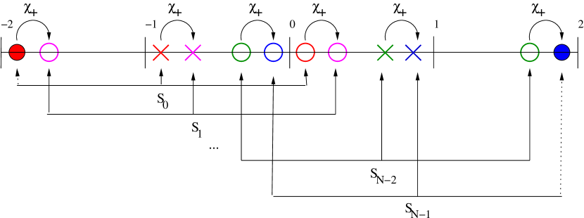
Figure 1: Action of $\chi_{\pm}$ on the eigenvalues: $\chi_{\pm}$ is the mapping between surfaces $X_{k\pm 1}.$ Its action is denoted by the arrows. The filled circles are “ghost” eigenvalues and the empty circles correspond to eigenvalues which are realized for some $k$. Here we have omitted the sets $S_{2}$ through $S_{N-2}$ as denoted by the ellipses.

Let us consider the set $S$ of all eigenvalues of immersion functions, $X_{k}$ for $k=0,...,N-1$ for a fixed $N.$ Further, let us define the following sets

$$\begin{array}[]{l}D^{+}\equiv\{c_{k}\}=\left\{\left.\frac{1}{N}+\frac{2k}{N}\right|k=0,1,..,N-2\right\},\\ D^{0}\equiv\{c_{k}-1\}=\left\{\left.\frac{1-N}{N}+\frac{2k}{N}\right|k=0,..,N-1\right\},\\ D^{-}\equiv\{c_{k}-2\}=\left\{\left.\frac{1-2N}{N}+\frac{2k}{N}\right|k=1,..,N-1\right\},\end{array}$$ (61)

and

$$D\equiv D^{+}\cup D^{-},\qquad S\equiv D\cup D^{0}.$$ (62)

Proposition 3

For the sets $D^{\pm}$ and $D^{0}$ defined above, we have the following restrictions, for all $N$

$$D^{+}\subset[\frac{1}{N},2-\frac{3}{N}],$$

$$D^{0}\subset[-1+\frac{1}{N},1-\frac{1}{N}],$$

$$D^{-}\subset[-2+\frac{3}{N},-\frac{1}{N}].$$

Proof: These follow from direct observations. The lowest element of $D^{+}$ is achieved for $k=0$ and has a value of $\frac{1}{N}$ whereas the highest element is achieved for $k=N-2$ and has the value of $2-\frac{3}{N}.$ The lowest element of $D^{0}$ is achieved for $k=0$ and has a value of $-1+\frac{1}{N},$ whereas the highest element is achieved for $k=N-1$ and has the value of $1-\frac{1}{N}.$ The lowest element of $D^{-}$ is achieved for $k=1$ and has a value of $-2+\frac{1}{N}$ whereas the highest element is achieved for $k=N-1$ and has the value of $-\frac{1}{N}.$ Also note that

$$S=D^{+}\cup D^{0}\cup D^{-}\subset[-2+\frac{3}{N},2-\frac{3}{N}],$$

and the distance between the highest and lowest eigenvalue is $d=2(2-\frac{3}{N}).$

$\square$

3.1.1 Symmetries of the sets $D^{\pm}$ and $D^{0}$

Here we shall prove that $D^{0}$ is symmetric about the origin and that the image of $D^{+}$ under multiplication by $-1$ is $D^{-},$ i.e. for any $x\in D^{+},$ $-x\in D^{-}.$

Proposition 4

$D^{0}$ is symmetric about the origin.

Proof: Let $x\in D^{0}$. Then

$$x = \frac{1-N+2k}{N},$$

$$-x = \frac{1-N-2l}{N},\qquad l=N-k-1.$$

This implies that $-x\in D^{0}.$

$\square$

Proposition 5

For any $x$ in $D^{+},$ $-x\in D^{-}.$

Proof: Let $x\in D^{+}.$

$$x = \frac{2k+1}{N},$$

$$-x = \frac{1-2N+2l}{N},\qquad l=N-k.$$

This implies that $-x\in D^{-}$

$\square$

3.1.2 Intersections of the sets $D^{\pm}$ and $D^{0}$

Here we claim that, for $N$ even, $D^{0}\subset D$ and, for $N$ odd, $D\cap D^{0}=\emptyset.$

Proposition 6

For $N$ odd, $D^{0}\cap D=\emptyset.$

Proof: Let $x\in D^{0}$ and $N=2n+1,$ then

$$x=\frac{1+2k-2n-1}{2n+1}.$$

Now, if $x\in D^{+}$ there exists some $k$ such that

$$\frac{2k-2n}{2n+1}=\frac{1+2k}{2n+1},$$

which is impossible because of the parity of the numerators. On the other hand, for $x$ to be in $D^{-}$ we require

$$\frac{2k-2n}{2n+1}=\frac{1+2k-4n-2}{2n+1},$$

which is also a contradiction because of the parity of the numerators. Thus, $D^{0}\cap D=\emptyset.$

$\square$

Proposition 7

For $N$ even, $D^{0}\subset D$

Proof: Suppose that $N$ is even, i.e. $N=2n$ with $n=1....$ Let $x\in D^{0},$ then

$$x = \frac{1-2n+2k}{2n},\qquad k\in\{0,..,2n\}.$$

Suppose also, without loss of generality, that $x\geq 0$ then $k$ must be greater than $n$ and so it is possible to define $l=k-n$. Since $n\geq k\leq 2n-1,$ $0\geq l=k-n\leq 2n-2$ and so

$$x=\frac{1+2l}{2n},\qquad l=k-n\in\{0,..,2n-2\}.$$

That is, $x\in D^{+}.$ By the symmetry arguments in Section 3.2, if $x$ is negative then $x\in D^{-}$ and so in either case $x\in D=D^{+}\cup D^{-}.$

$\square$

3.1.3 Spacing between elements of $S$

It can be directly observed from the definition of the $c_{k}$’s that the difference between each $c_{k}$ is $2/N.$ Thus the spacing between elements in $D^{+}$, $D^{-}$ and $D^{0}$ is always $2/N.$

Proposition 8

For $N$ even, the step size between elements of $S$ is $2/N$.

Proof: From Proposition 7, $D^{0}\subset D$ and so $S=D.$ Further, we know that $D^{+}\subset[\frac{1}{N},2-\frac{3}{N}]$ and $D^{-}\subset[-2+\frac{3}{N},-\frac{1}{N}]$ and so these sets are disjoint and the elements within each of them are at a distance $2/N$ apart. Finally, the highest element of $D^{-}$ is $-1/N$ and the lowest element of $D_{+}$ is $1/N$ and so they are at a distance of $2/N$ apart. Thus, all elements of $S$ are at a distance of $2/N$ from their nearest neighbor.

$\square$

Proposition 9

For $N$ odd, on the interval $[-1,1]$, the step size between elements of $S$ is $1/N.$ On the intervals $[1,2-\frac{3}{N}]$ and $[-2+\frac{3}{N},-\frac{1}{N}]$ the step size is $2/N.$

Proof: First we show that, for $N$ odd, $1\in D^{+}$ and $-1\in D^{-}.$ Assume that $N=2n+1,$ then

$$1=\frac{1}{2n+1}+\frac{2n}{2n+1}=c_{n}\in D^{+},$$

$$-1=1-2=c_{n}-2\in D^{-}.$$

Thus, for $N=2n+1$ odd,

$$D\cap[-1,1] =\left\{-1,-1+\frac{2}{2n+1},...,1-\frac{2}{2n+1},1\right\}$$

$$=\left\{\left.-1+\frac{2\ell}{2n+1}\right|\ell=1,...,2n+1\right\}.$$

On the other hand

$$D^{0}=\left\{\left.-1+\frac{2\ell+1}{2n+1}\right|\ell=1,...,2n+1\right\},$$

and so, for $N$ odd,

$$S\cap[-1,1] = (D\cap[-1,1])\cup D^{0}$$

$$= \left\{\left.-1+\frac{k}{2n+1}\right|k=1,...,2n+1\right\},$$

and in particular, the difference between the energy values is $1/N.$

However, on the intervals $[1,2-\frac{3}{N}]$ and $[-2+\frac{3}{N},-\frac{1}{N}],$ $S$ is comprised solely of $D^{+}$ and $D^{-}$ respectively and so the the step size is $2/N$ as remarked above.

$\square$

3.1.4 Counting elements of S

Define $|A|$ to be the number of elements in the set, then the following identities hold:

$$D^{+}\cap D^{-}=\emptyset,\qquad|D^{+}|=N-1,\quad|D^{-}|=N-1.$$

We can immediately see that:

1. If $N$ is odd,

   $$|S|=|D|+|D^{0}|=2N-2+N=3N-2.$$

2. If $N$ is even,

   $$|S|=|D|=2N-2.$$

Note that, counting repeated eigenvalues, the number of eigenvalues is $3N-2$. For $N$ odd, as was proven in Proposition 6, no eigenvalues are repeated and so there are $3N-2$ distinct eigenvalues. For $N$ even, as was proven in Proposition 7, all of the values in $D^{0}$ are also in $D$ and so there are $N$ repeated eigenvalues (i.e. shared by two different surfaces) and so only $2N-2$ are distinct.

3.1.5 Graphs

Let us display the eigenvalues of $X_{k}$ for $k=0,\ldots,N-1$, i.e. the set $S=D\cup D^{0}$, on the real line in the following graphs, figures 2 and 3. Here we represent the elements of $D$ by dots and the elements of $D^{0}$ by $x$’s. We also include the two “ghost” values of dots by filled in circles. Note that the set of points distributed along the real line is symmetric with respect to the origin. Therefore, it is sufficient to consider only the right or left half of the set $S$.

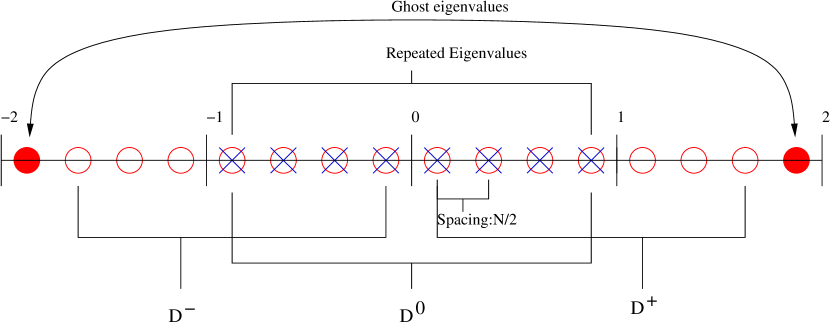
Figure 2: Eigenvalues for $N=8$ (even): The elements of $D$ are represented by hollow dots and the eigenvalues of $D^{0}$ are represented by $x$’s. The filled in circles represent ghost eigenvalues.

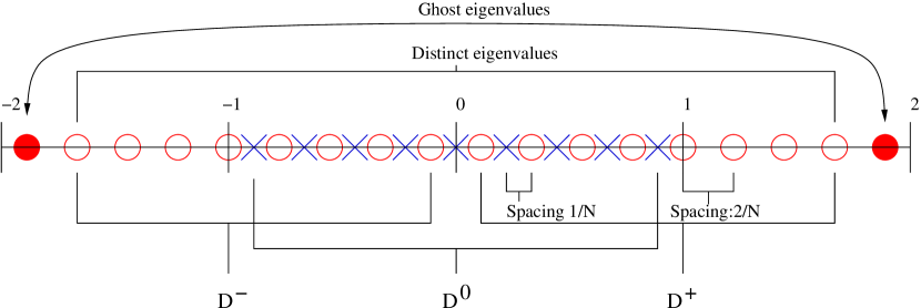
Figure 3: Eigenvalues for $N=9$ (odd): The elements of $D$ are represented by hollow dots and the eigenvalues of $D^{0}$ are represented by $x$’s. The filled in circles represent ghost eigenvalues.

3.2 Mapping between sets of eigenvalues for different $N$

The question to be answered in this section is whether there exists an operator $A_{\pm}$ such that

$$A_{+}S(N)=S(N+1),\qquad A_{-}S(N)=S(N-1),$$

which lowers or raises the number of dots? Here the answer is affirmative.

Recall, the eigenvalues of each surface $X_{k}$ depend on the dimension of the space $N$

$$S_{k}(N)=\{c_{k},c_{k}-1,c_{k}-2\},\qquad c_{k}=\frac{1+2k}{N},$$

and hence the union of these values depends on $N$ not only in the summation but also in the values of the individual $S_{k}$’s i.e.

$$S(N)=S=\bigcup_{k=0}^{N-1}S_{k}(N).$$

In this section, we will outline a simple procedure for performing the induction on $N$ which maps from $S(N)$ to $S(N\pm 1)$. Let us consider the sets $D^{\pm}$ and $D^{0}$ and describe them in a way that is conducive to performing induction on $N$. We denote $D^{\pm}=D^{\pm}(N)$ and $D^{0}=D^{0}(N)$ to make explicit the dependence on $N$.

We describe each set in the following way. For each set, we place in the interval $M$ points such that

• the points are evenly spaced throughout the interval at a maximal distance

• the points are at least a distance $1/M$ from the end points of the interval where $M$ is the number of points in the interval.

Thus, $D^{-}(N)$ is the set of $N$ points satisfying conditions 1 and 2, where $M=N,$ on the interval $[-2,0]$ where the lowest point is designated a “ghost” point. Similarly, $D^{+}(N)$ is the set of $N$ points satisfying conditions 1 and 2 on the interval $[0,2]$ where the highest point is designated a “ghost” point. The set $D^{0}(N)$ is the set of $N$ points on the interval $[-1,1]$ satisfying conditions 1 and 2. Then

$$S(N)=D^{-}(N)\cup D^{0}(N)\cup D^{+}(N).$$

The same conditions hold for $M=N+1.$ That is $D^{-}(N+1)$ is the set of $N+1$ points satisfying conditions 1 and 2 on the interval $[-2,0]$ where the lowest point is designated a “ghost” point. Similarly, $D^{+}(N+1)$ is the set of $N+1$ points satisfying conditions 1 and 2 on the interval $[0,2],$ where the highest point is designated a “ghost” point. The set $D^{0}(N+1)$ is the set of $N+1$ points on the interval $[-1,1]$ satisfying conditions 1 and 2. Then

$$S(N+1)=D^{-}(N+1)\cup D^{0}(N+1)\cup D^{+}(N+1).$$

With this description we can immediately see the induction step. To describe $S(N+1)$ in terms of the configurations of $S(N)$, we need only add a point to each interval and require the same conditions, 1 and 2, on the arrangement of the points. For the set $S(N-1)$ we subtract one point from each interval and require that 1 and 2 hold.

Note that this description does not depend on the parity of $N$ and in particular, the points in each set may overlap, depending on the parity of $N$, and result in repeated eigenvalues.

3.3 Completeness of the set of eigenvalues

It is apparent that the surfaces $X_{k},~{}k=0,\dots,N\!-\!1$ are too few to make a basis in the Lie algebra $\mathop{\mathfrak{su}(N)}\nolimits$. However, for each $(\xi,\overline{\xi})\in\Omega\subset{{\mathbb{C}}},$ we have the following result,

Proposition 10

1. The vector subspace spanned by the surfaces $X_{k}~{}(k=0,\dots N\!-\!1)$, exhausts all the possible spectra for elements of the Lie algebra $\mathop{\mathfrak{su}(N)}\nolimits$.

2. The projectors $P_{k}$ are not traceless, therefore they span a larger subspace, whose spectra may assume all the values from $\mathbb{C}^{N}$.

Proof: The surfaces $X_{k}$ as well as the projectors $P_{k}$ are diagonalizable (the first ones as antihermitian matrices, the second ones as hermitian matrices). As before, let $V$ be the diagonalizing matrix for the projectors (31) and let $\lambda_{0},...,\lambda_{N-1}$ be an arbitrary sequence of complex numbers. Consider a linear combination of the projectors

$$S=\sum_{k=0}^{N-1}\lambda_{k}P_{k}=V^{-1}\left(\sum_{k=0}^{N-1}\lambda_{k}\mathbb{I}_{k}\right)V.$$

The matrix S has eigenvalues $\lambda_{0},\ldots\lambda_{N}$ and so this completes the proof of the part part (ii) of the proposition. Part part (i) follows from the fact that each of the projectors $P_{k}$ may be expressed as a linear combination of the traceless matrices $X_{k},~{}k=1,\dots,N\!-\!1$ and the unit matrix $\mathbb{I}$ (14). Thus the matrix $S$ can be expressed as a linear combination of the $X_{k}$’s and the unit matrix. The eigenvalues satisfy $\lambda_{0}+\ldots\lambda_{N-1}=0$ if and only if $S$ is traceless and so the coefficient of $\mathbb{I}$ is zero. Hence the matrix $S$ is a linear combination of $X_{k}$ and thus it is an element of the subalgebra spanned by the $X_{k}$.

$\square$

Similarly, we have the following result.

Proposition 11

Each diagonalizable $N\!\times\!N$ matrix is conjugate to a linear combination of the projectors $P_{k},~{}k=0,\dots N\!-\!1$; each $\mathop{\mathfrak{su}(N)}\nolimits$ matrix is conjugate to a linear combination of the surfaces $X_{k},\quad k=0,\dots N\!-\!1$.

Proof: Indeed, let $W$ be the diagonalizing matrix of a given $N\!\times\!N$ matrix $M$, i. e.

$$W^{-1}MW=\sum_{k=0}^{N-1}\lambda_{k}\mathbb{I}_{k}.$$

Again, the matrix $V$ (31) is the matrix which diagonalizes the projectors $P_{k}$ and so

$$M=WV^{-1}\left(\sum_{k=0}^{N-1}\lambda_{k}P_{k}\right)VW^{-1}.$$

If we limit the sequences to those which satisfy $\lambda_{0}+\ldots\lambda_{N-1}=0$, a similar argument shows that each of the $\mathop{\mathfrak{su}(N)}\nolimits$ matrices is conjugate to a linear combination of the surfaces $X_{k}$.

$\square$

The matrices which represent spins are subalgebras of $\mathop{\mathfrak{su}(N)}\nolimits$ ; more specifically, the usual quantum mechanics spins are representations of $\mathop{\mathfrak{su}(2)}\nolimits$ in $\mathbb{C}^{N}$. The eigenvalues of a matrix representing particles of spin $s$ are $-s,-s+1,\dots,s$. Hence $s=(N-1)/2$. For such matrices we have the following.

Proposition 12

The matrices which represent spins are conjugate to $-(i/2)\sum_{k=0}^{N-1}X_{k}$, i. e. every spin field is conjugate, up to the factor $-i/2$, to a sum of all the surfaces $X_{k},\,k=0,\dots,N\!-\!1$.

Proof: Substituting $X_{k}$ from (13) into $-(i/2)\sum_{k=0}^{N-1}X_{k}$, expressing the unit matrix inherent in (13) as a sum of all the projectors $\mathbb{I}=\sum_{k=0}^{N-1}P_{k}$, and collecting the terms at each of $P_{k}$, we obtain

$$-\frac{i}{2}\sum\limits_{k=0}^{N-1}X_{k}=\sum\limits_{k=0}^{N-1}\left(-\frac{1}{2}P_{k}-\sum\limits_{j=0}^{k-1}P_{j}+\frac{1+2k}{2\,N}\sum\limits_{j=0}^{N-1}P_{j}\right)=\sum\limits_{k=0}^{N-1}\left(-\frac{N-1}{2}+k\right)P_{k}\,.$$ (63)

According to the above Proposition, the expression on the right-hand-side is conjugate to any $\mathop{\mathfrak{su}(N)}\nolimits$ matrix whose eigenvalues are $-(N-1)/2,-(N-1)/2+1,\dots,(N-1)/2$.

$\square$

Finally, note that the surface immersion functions $X_{k}$ span a Cartan subalgebra of the $\mathop{\mathfrak{su}(N)}\nolimits$ algebra, i.e. not only do all the $X_{k}$ commute with one another, but also any $N\!\times\!N$ matrix which commutes with all the $X_{k},~{}k=0,...,N\!-\!1$ is their linear combination. The latter property stems directly from the fact that being a Cartan subalgebra is invariant under conjugation, while the $X_{k}$ are conjugate to the Abelian Lie algebra of diagonal traceless $N\!\times\!N$ matrices.

4 Conclusion

In this paper, we considered soliton surfaces associated with ${{{\mathbb{C}}}P^{N-1}}$ sigma models. We show (Proposition 1) that the GWFI for surfaces associated with ${{{\mathbb{C}}}P^{N-1}}$ sigma models with finite action defined on the Riemann sphere satisfies the E-L equations (30) Such surfaces are known to be conformally parameterized and to have surface area proportional to the action functional. Conversely, we have shown (Proposition 2) that the immersion functions into $\mathop{\mathfrak{su}(N)}\nolimits$ in conformal coordinates that are extremals of the area functional subject to any polynomial identity satisfy the same E-L equations (30). This discussion emphasized the importance of the eigenvalues of the immersion functions in determining the class of solutions. In particular, an immersion function $X$ is given by the GWFI for solutions of the ${{{\mathbb{C}}}P^{N-1}}$ sigma models with finite action defined on the Riemann sphere if and only if it satisfies the E-L equations (30) and has eigenvalues as indicated by (16), (17) and (18).

These quantized eigenvalues have a rich structure which was elucidated in Section 3. In that section, we performed a systematic analysis of the eigenvalues, including the action of the raising and lowering operators ($X_{k}\rightarrow X_{k\pm 1}$) on the eigenvalues. We also described the symmetries in the distribution as well as degeneracies of eigenvalues. Finally, we discussed the distributions of eigenvalues for different dimensions ($N$). Additionally, we show that any diagonalizable matrix is conjugate to a linear combination of the projectors and any $\mathop{\mathfrak{su}(N)}\nolimits$ matrix is conjugate to a linear combintation of the surfaces $X_{k}$; in particular matrices which represent spins can be written as a linear combination of the $X_{k}$’s. Furthermore, the immersion functions $X_{k}$ form a Cartan subalgebra of $\mathop{\mathfrak{su}(N)}\nolimits$.

In the future, it would be interesting to consider a physical interpretation for these eigenvalues in connection with spin statistics as well as the connections with the orthogonal polynomials associated with these distributions. These topics will be explored in our future work.

References

References

- [1] Bobenko A 1994 Surfaces in terms of 2 by 2 matrices Harmonic Maps and Integrable systems, eds. A Fordy and J C Wood (Braunschweig: Vieweg)
- [2] Callan C G, Coleman S, Wess J and Zumino B 1969 Structure of phenomenological Lagrangians. II Phys. Rev. 177 2247–2250
- [3] Carrol R and Konopelchenko B 1996 Generalized Weierstrauss-Enneper inducing conformal immersions and gravity Int. J. Mod. Phys. 11 1183–1261
- [4] Coleman S, Wess J and Zumino B 1969 Structure of phenomenological Lagrangians. I Phys. Rev. 177 2239–2247
- [5] David F, Ginsparg P and Zinn-Justin Y, eds. 1996 Fluctuation Geometries in Statistical Mechanics and Field Theory (Amsterdam: Elsevier)
- [6] Davydov A 1999 Solitons in Molecular Systems (New York: Springer)
- [7] Din A M and Zakrzewski W J 1980 General classical solutions in the model Nucl. Phys. B 174 397–406
- [8] Gell-Mann M and Lévy M 1960 The axial vector current in beta decay Nuovo Cimento 16 1729–50
- [9] Goldstein P P and Grundland A M 2009 Invariant formulation of surfaces associated with models Arxiv 10022906
- [10] Goldstein P P and Grundland A M 2010 Invariant recurrence relations for models. J. Phys. A 43 265206
- [11] Goldstein P P and Grundland A M 2011 Invariant description of sigma models Theor. Math. Phys. 168 939–950
- [12] Goldstein P P and Grundland A M 2011 On the surfaces associated with models Journal of Physics: Conference Series 284 012031
- [13] Gross D G, Piran T and Weinberg S 1992 Two Dimensional Quantum Gravity and Random Surfaces (Singapore: World Scientific)
- [14] Grundland A M and Post S 2011 Solition surfaces associated with generalized symmetries of integrable equations. J. Phys. A 44 165203
- [15] Grundland A M and Post S 2012 Soliton surfaces via zero-curvature representation of differential equations J. Phys. A 45 115204
- [16] Grundland A M, Strasburger A and Zakrzewski W 2005 Surfaces immersed in Lie algebras obtained from sigma models. J. Phys. A 39 9187–9213
- [17] Grundland A M and Yurdusen I 2009 On analytic discriptions of two-dimensional surfaces associated with the sigma models. J. Phys. A 42 172001
- [18] Guest M A 1997 Harmonic Maps, Loop groups and Integrable systems. (Cambridge: Cambridge University Press)
- [19] Helein F 2002 Harmonic Maps, Conservation Laws and Moving Frames (Cambridge: Cambridge University Press)
- [20] Konopelchenko B 1996 Induced surfaces and their integrable dynamics. Stud. Appl. Math. 96 9–51
- [21] Konopelchenko B and Landolfi G 1999 Induced surfaces and their integrable dynamics: II. Generalized Weierstrauss representations in 4-d spaces and deformations via DS hierarchy. Stud. Appl. Math. 96 129–169
- [22] Konopelchenko B and Taimanov I 1996 Constant mean curvature surfaces via an integrable dynamical system J. Phys. A 29 1261–1265
- [23] Landolfi G 2003 On the Canham-Helfrich membrane model. J. Phys. A 36 4699–4715
- [24] Manton N and Sutcliffe P 2004 Topological Solitons Cambridge Monographs on Mathematical Physics (Cambridge: Cambridge University Press)
- [25] Mikhailov A V 1986 Integrable magnetic models Solitons, vol. 17 of Modern Problems in Condensed Matter, eds. S E Trullinger, V E Zakharov and V L Pokrovsky (Amsterdam: North-Holland) pp. 623–690
- [26] Nelson D, Piran T and Weinberg S 1992 Statistical Mechanics of Membranes and Surfaces (Singapore: World Scientific)
- [27] Ou-Yang Z, Lui J and Xie Y 1999 Geometric Methods in Elastic Theory of Membranes in Liquid Crystal Phases (Singapore: World Scientific)
- [28] Polchinski J and Strominger A 1991 Effective string theory Phys. Rev. Lett. 67 1681–1684
- [29] Polyakov A M 1987 Gauge Fields and Strings (New Jersey: Harwood Academic)
- [30] Post S and Grundland A M 2012 Analysis of sigma models via projective structure Nonlinearity 25 1
- [31] Sasaki R 1983 General class of solutions of the complex Grassmannian and sigma models. Phys. Lett. B 130 69–72
- [32] Uhlenbeck K 1989 Harmonic maps into Lie groups (classical solutions of the Chiral model) J. Diff. Geom. 30 1–50
- [33] Ward R 1994 Sigma models in 2+1 dimensions Harmonic Maps and Integrable Systems, eds. A Fordy and J C Wood (Braunschweig: Vieweg)
- [34] Zakharov V E and Mikhailov A V 1979 Relativistically invariant two-dimensional models of field theory which are integrable by means of the inverse scatterting method. Sov. Phys. JETP 40 1017–1049
- [35] Zakrzewski W J 1989 Low Dimensional Sigma Models (Bristol: Adam Hilger)