Abstract

Ability to find and get services is a key requirement in the development of large-scale distributed systems. We consider dynamic and unstable environments, namely Peer-to-Peer (P2P) systems. In previous work, we designed a service discovery solution called Distributed Lexicographic Placement Table (Dlpt), based on a hierarchical overlay structure. A self-stabilizing version was given using the Propagation of Information with Feedback (PIF) paradigm. In this paper, we introduce the self-stabilizing CoPIF (for Collaborative PIF) scheme. An algorithm is provided with its correctness proof. We use this approach to improve a distributed P2P framework designed for the services discovery. Significantly efficient experimental results are presented.

1 Introduction

Computing abilities (or services) offered by large distributed systems are constantly increasing. Cloud environment grows in this way. Ability to find and get these services (without the need for a centralized server) is a key requirement in the development of such systems. Service discovery facilities in distributed systems led to the development of various overlay structures built over Peer-to-Peer (P2P) systems, e.g., [12, 18, 26, 27]. Some of them rely on spanning tree structures [12, 27], mainly to handle range queries, automatic completion of partial search strings, and to extend to multi-attribute queries.

Although fault-tolerance is a mandatory feature of systems targeted for large scale platforms (to avoid data loss and to ensure proper routing), tree-based distributed structures, including tries, offer only a poor robustness in dynamic environment. The crash of one or more nodes may lead to the loss of stored objects, and may split the tree into several subtrees.

The concept of self-stabilization [16] is a general technique to design distributed systems that can handle arbitrary transient faults. A self-stabilizing system, regardless of the initial state of the processes and the initial messages in the links, is guaranteed to converge to the intended behavior in finite time.

In [10], a self-stabilizing message passing protocol to maintain prefix trees over practical P2P networks is introduced. The protocol is based on self-stabilizing PIF (Propagation of Information with Feedback) waves that are used to evaluate the tree maintenance progression. The scheme of PIF can be informally described as follows: a node, called initiator, initiates a PIF wave by broadcasting a message m into the network. Each non-initiator node acknowledges to the initiator the receipt of m. The wave terminates when the root has received an acknowledgment from all other nodes. In arbitrary distributed systems, any node may need to initiate a PIF wave. Thus, any node can be the initiator of a PIF wave and several PIF protocols may run concurrently (in that case, every node maintains locally a data structure per initiator).

Contribution.

We first present the scheme of collaborative PIF (referred as CoPIF). The main thrust of this scheme is to ensure that different waves may collaborate to improve the overall parallelism of the mechanism of PIF waves. In other words, the waves merge together so that they do not have to visit parts of the network already visited by other waves. Of course, this scheme is interesting in environments were several PIF waves may run concurrently. Next, we provide a self-stabilizing CoPIF protocol with its correctness proof. To the best of our knowledge, it is the first self-stabilizing solution for this problem. Based on the snap-stabilizing PIF algorithm in [8], it merges waves initiated at different points in the network. In the worst case where only one PIF wave runs at a time, our scheme does not slow down the normal progression of the wave. Finally, we present experimental results showing the efficiency of our scheme use in a large scale P2P tree-based overlay designed for the services discovery.

Roadmap.

The related works are presented in Section 2. Section 3 provides the conceptual and computational models of our framework. In Section 4, we present and prove the correctness of our self-stabilizing collaborative protocol. In Section 5, experiments show the benefit of the CoPIF approach. Finally, concluding remarks are given in Section 6.

2 Related Work

2.1 Self-stabilizing Propagation of Information

PIF wave algorithms have been extensively proposed in the area of self-stabilization, e.g., [2, 5, 8, 14, 30] to quote only a few. Except [5, 14, 30], all the above solutions assume an underlying self-stabilizing rooted spanning tree construction algorithm. The solutions in [8, 14] have the extra desirable property of being snap-stabilizing. A snap-stabilizing protocol guarantees that the system always maintains the desirable behavior. This property is very useful for wave algorithms and other algorithms that use PIF waves as the underlying protocols. The basic idea is that, regardless of the initial configuration of the system, when an initiator starts a wave, the messages and the tasks associated with this wave will work as expected in a normal computation. A snap-stabilizing PIF is also used in [11] to propose a snap-stabilizing service discovery tool for P2P systems based on prefix tree.

2.2 Resource Discovery

The resource discovery in P2P environments has been intensively studied [20]. Although DHTs [24, 25, 28] were designed for very large systems, they only provide rigid mechanisms of search. A great deal of research went into finding ways to improve the retrieval process over structured peer-to-peer networks. Peer-to-peer systems use different technologies to support multi-attribute range queries [6, 18, 26, 27]. Trie-structured approaches outperform others in the sense that logarithmic (or constant if we assume an upper bound on the depth of the trie) latency is achieved by parallelizing the resolution of the query in several branches of the trie.

2.3 Trie-based related work

Among trie-based approaches, Prefix Hash Tree (PHT) [22] dynamically builds a trie of the given key-space (full set of possible identifiers of resources) as an upper layer mapped over any DHT-like network. Fault-tolerance within PHT is delegated to the DHT layer. Skip Graphs, introduced in [3], are similar to tries, and rely on skip lists, using their own probabilistic fault-tolerance guarantees. P-Grid is a similar binary trie whose nodes of different sub-parts of the trie are linked by shortcuts like in Kademlia [19]. The fault-tolerance approach used in P-Grid [15] is based on probabilistic replication.

In our approach, the Dlpt was initially designed for the purpose of service discovery over dynamic computational grids and aimed at solving some drawbacks of similar previous approaches. An advantage of this technology is its ability to take into account the heterogeneity of the underlying physical network to build a more efficient tree overlay, as detailed in [13].

3 P2P Service Discovery Framework

In this section we present the conceptual model of our P2P service discovery framework and the Dlpt data structure on which it is based. Next, we convert our framework into the computational model on which our proof is based.

3.1 Conceptual Model

The two abstraction layers that compose our P2P service discovery framework are organized as follow: ($i$) a $P2P$ network which consists of a set of asynchronous peer (physical machines) with distinct identifiers. The peer communicate by exchanging messages. Any peer $P1$ is able to communicate with another peer $P2$ only if $P1$ knows the identifier of $P2$. The system is seen as an undirected graph $G=(V,E)$ where $V$ is the set of peers and $E$ is the set of bidirectional communication link; ($ii$) an overlay that is built on the P2P system, which is considered as an undirected connected labeled tree $G^{\prime}=(V^{\prime},E^{\prime})$ where $V^{\prime}$ is the set of nodes and $E^{\prime}$ is the set of links between nodes. Two nodes $p$ and $q$ are said to be neighbors if and only if there is a link $(p,q)$ between the two nodes. To simplify the presentation we refer to the link $(p,q)$ by the label $q$ in the code of $p$. The overlay can be seen as an indexing system whose nodes are mapped onto the peers of the network. Henceforth, to avoid any confusion, the word node refers to a node of the tree overlay, i.e., a logical entity, whereas the word peer refers to a physical node part of the $P2P$ system.

Reading and writing features of our service discovery framework are ensured as follow. Nodes are indexed with service name and resource locations are stored on nodes. So, client requests are treated by any node, rooted to the targeted service labeled node along the overlay abstraction layer, indexed resource locations are returned to the clients or updated . A more detailed description of the implementation of our framework is given in [9] and briefly reminded in Section 5.1.

The Distributed Lexicographic Placement Table (Dlpt [12, 13]) is the hierarchical data structure that ensures request routing across overlay layer. Dlpt belongs to the category of overlays that are distributed prefix trees, e.g.,  [4, 23, 1]. Such overlays have the desirable property of efficiently supporting range queries by parallelizing the searches in branches of the tree and exhibit good complexity properties due to the limited depth of the tree. More particularly, Dlpt is based on the particular Proper Greatest Common Prefix Tree (Pgcp tree) overlay structure. A Proper Greatest Common Prefix Tree (a.k.a radix tree in [21]) is a labeled rooted tree such that the following properties are true for every node of the tree: ($i$) the node label is a proper prefix of any label in its subtree; ($ii$) the greatest common prefix of any pair of labels of children of a given node are the same and equal to the node label.

Designed to evolve in very dynamic systems, the Dlpt integrates a self-stabilization mechanisms [10], providing the ability to recover a functioning state after arbitrary transient failures. As such, the truthfulness of information returned to the client needs to be guaranteed. We use the PIF mechanism to check whether Dlpt is currently in a recovering phase or not.

3.2 Computational Model

In a first step, we abstract the communication model to ease the reading and the explanation of our solution. We assume that every pair of neighboring nodes communicate in the overlay by direct reading of variables. So, the program of every node consists in a set of shared variables (henceforth referred to as variables) and a finite number of actions. Each node can write in its own variables and read its own variables and those of its neighbors. Each action is constituted as follow: $<Label>::<Guard>\rightarrow<Statement>$. The guard of an action is a Boolean expression involving the variables of $p$ and its neighbors. The statement is an action which updates one or more variables of the node $p$. Note that an action can be executed only if its guard is true. Each execution is decomposed into steps. Let $y$ be an execution and $A$ an action of $p$ ($p$ $\in$ $V$). $A$ is enabled for $p$ in $y$ if and only if the guard of $A$ is satisfied by $p$ in $y$. Node $p$ is enabled in $y$ if and only if at least one action is enabled at $p$ in $y$.

The state of a node is defined by the value of its variables. The state of a system is the product of the states of all nodes. The local state refers to the state of a node and the global state to the state of the system. Each step of the execution consists of two sequential phases atomically executed: ($i$) Every node evaluates its guard; ($ii$) One or more enabled nodes execute their enabled actions. When the two phases are done, the next step begins.

Formal description (Section 4.2) and proof of correctness of the proposed collaborative propagate information feedback algorithm will be done using this computational model. Nevertheless, experiments are implemented using the classical message-passing model over an actual peer-to-peer system [7, 17].

4 Collaborative Propagation of Information with Feedback Algorithm

In this section, we first present an overview of the proposed Collaborative Propagation of Information with Feedback Algorithm (CoPIF). Next, we provide its formal description.

4.1 Overview of the CoPIF

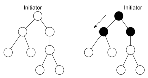
(a) Broadcast step.

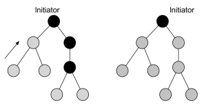
(b) Feedback step.

Figure 1: The PIF Wave.

Before explaining the idea behind CoPIF, let us first recall the well-known PIF wave execution. Starting from a configuration where no message has been broadcast yet, a node, also called initiator, initiates the broadcast phase and all its descendant except the leaf participate in this task by sending also the broadcast message to their descendants. Once the broadcast message reaches a leaf node of the network, they notify their ancestors of the end of the broadcast phase by initiating the feedback phase. During both broadcast and feedback steps, it is possible to collect information or perform actions on the entire data structure. Once all the nodes of the structure have been reached and returned the feedback message, the initiator retrieve collected information and executes a special action related to the termination of the PIF-wave. In the sequel, we will refer to this mechanism as classic-PIF.

However, the PIF mechanism is a costly broadcast mechanism that involves the whole platform. In this paper, we aim to increase the parallelism of the PIF by making several PIF waves collaborating together. Let us now define some notions that will be used in the description of our solution:

Let an ordered alphabet $A$ be a finite set of letters. Lets define $\prec$ an order on $A$. A non empty word $w$ over $A$ is a finite sequence of letters $a_{1}$, … , $a_{i}$, …, $a_{l}$ such as $l>0$. The concatenation of two words $u$ and $v$, denoted as $uv$, is equal to the word $a_{1}$, …, $a_{i}$, …, $a_{k}$, $b_{1}$, …, $b_{j}$, …, $b_{l}$ such that $u=a_{1}$, …, $a_{i}$, …, $a_{k}$ and $v=b_{1}$, …, $b_{j}$, …, $b_{l}$. A word $u$ is a prefix (respectively, proper prefix) of a word $v$ if there exists a word $w$ such that $v=uw$ (respectively, $v=uw$ and $u\neq v$). The Greatest Common Prefix (respectively, Proper Greatest Common Prefix) of $w_{1}$ and $w_{2}$, denoted $GCP(w_{1},w_{2})$ (respectively $PGCP(w_{1},w_{2})$, is the longest prefix $u$ shared by $w_{1}$ and $w_{2}$ (respectively, such that $\forall i\geq 1$, $u\neq w_{i}$).

Let us now describe the outline of the proposed solution through the P2P framework use case.

Use Case.

The idea of the algorithm is the following: When a user is looking for a service, it sends a request to the Dlpt to check whether the service exists or not. Once the request is on one node of the Dlpt, it is routed according to the labelled tree in the following manner: let $l_{request}$ be the label of the service requested by the user and let $l_{p}$ be the label of the current node $u_{p}$. In the case of $PGCP(l_{request},l_{p})$ is true, $u_{p}$ checks whether there exists a child $u_{q}$ in the Dlpt having a label $l_{q}$ such that $PGCP(l_{request},l_{q})$ is satisfied. If such a node exists, then $u_{p}$ forwards the request to its child $u_{q}$. Otherwise ($PGCP(l_{request},l_{p})$ is not satisfied), if we keep exploring the sub-tree routed in $u_{p}$, the service will not be found. $u_{p}$ sends in this case the request to its father node in the Dlpt. By doing so, either ($i$) the request is sent to one node $u_{p}$ such that $l_{p}=l_{request}$, or ($ii$) the request reaches a node $u_{p}$ such that it cannot be routed anymore. In the former case, the service being found, a message containing the information about the service is sent to the user. In the latter case, the service has not been found and the message “no information about the service” is sent to the user. However, the node has no clue to trust the received information or not. In other words, in the former case, $u_{p}$ does not know whether it contains the entire service information or if a part of the information is on a node being at a wrong position in the tree due to transient faults. In the latter case, $u_{p}$ does not know whether the service is really not supported by the system or if the service is missed because it is at a wrong position.

In order to solve this problem, $u_{p}$ initiates a PIF wave to check the state of all the nodes part of the Dlpt. Note that several PIF waves can be initiated concurrently since many requests can be made in different parts of the system. The idea of the solution is to make the different PIF waves collaborating in order to check whether the tree is under construction or not. For instance, assume that two PIF waves, $PIF1$ and $PIF2$, are running concurrently on two different parts of the tree, namely on the subtrees $T1$ and $T2$, respectively. Our idea is to merge $PIF1$ and $PIF2$ so that $PIF1$ (respectively, $PIF2$) do not traverse $T2$ (resp., $T1$) by using data collected by $PIF2$ (resp.$PIF1$). Furthermore, our solution is required to be self-stabilizing.

CoPIF.

Basically, the CoPIF scheme is a mechanism enabling the collaboration between different PIF waves. Each node $u_{p}$ of the Dlpt has a state variable $S_{p}$ that includes three parameters $S_{p}=(Phase,id_{f},id_{PIF})$. Parameter $id_{PIF}$ refers to the identifier of the PIF wave which consists of the couple ($id_{peer}$,$l_{u_{i}}$), where $id_{peer}$ is the identifier of the peer hosting the node $u_{i}$ that initiated the PIF wave and $l_{u_{i}}$ is the label of the node $u_{i}$. The value $id_{f}$ refers to the identifier of the neighbor from which $u_{p}$ received the broadcast. It is set at NULL in the case $u_{p}$ is the initiator. $Phase$ can have four values: $C$, $B$, $FC$ and $FI$. The value $C$ (Clean) denotes the initial state of any node before it participates in a PIF wave. The value $B$ (Broadcast) or $FC$ (Feedback correct) or $FI$ (Feedback incorrect) means that the node is part of a PIF wave. Observe that in the case there is just a single PIF wave that is executed on the Dlpt, then its execution is similar to the previously introduce classic-PIF.

When more than one PIF wave are executed, four cases are possible while the progression of the CoPIF wave. First ($i$), if there is a node $u_{p}$ in the $C$ state having only one neighboring node $q$ in the $B$ state and no other neighboring node in the $FI$ or $FC$ state, then $p$ changes its state to $B$. Second ($ii$), if there exists a leaf node $u_{p}$ in the $C$ state having a neighbor $u_{q}$ in the $B$ state, then $u_{p}$ changes its state to $FC$ (resp. $FI$) if its position in the Dlpt is correct (resp. incorrect). Next ($iii$), if there is a node $u_{p}$ in $C$-phase having two neighboring nodes $u_{q}$ and $u_{q^{\prime}}$ in the $B$ state with different $id_{PIF}$ then, $u_{p}$ changes its state to $B$ and sets its $id_{f}$ to $u_{q}$ such that the $id_{PIF}$ of $u_{q}$ is smaller than $id_{PIF}$ of $u_{q^{\prime}}$. Finally ($iv$), if there exists a node $u_{p}$ that is already in the $B$ state such that its $id_{f}$ is $u_{q}$ and there exists another neighboring node $u_{q^{\prime}}$ which is in the $B$ state with a smaller $id_{PIF}$ and a different $id_{f}$, then $u_{p}$ changes its father by setting $id_{f}$ at $u_{q^{\prime}}$.

Notice that in the fourth cases, $u_{q}$ (previously, the $id_{f}$ of $u_{p}$) will have to change its $id_{f}$ as well since it has now a neighbor $u_{p}$ in the $B$ state with a smaller $id_{peer}$. By doing so, the node $u_{i}$ that initiated a PIF wave with a smaller $id$ will change its $id_{peer}$. Similarly, notice that $u_{i}$ is not an initiator anymore. Hence it changes its $id_{f}$ from NULL to the $id$ of its neighbor with a smallest $id_{PIF}$. So, only one node will get the answer (the feedback of the CoPIF), this node being the one with the smallest $id_{PIF}$. Therefore, when an initiator sets its $id_{f}$ to a value different from NULL (as $u_{i}$ previously), it sends a message to the new considered initiator (can be deduced from $id_{PIF}$) to subscribe to the answer. So, when an initiator node receives the feedback that indicates the state of the tree, it notifies all its subscribers of the answer.

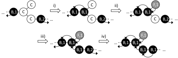
Figure 2: 4 CoPIF wave transition.

4.2 Formal Description

In the following we first define the data and variables that are used for the description of our algorithm. We then present the formal description in Algorithm 1.

• Predicates

  • $Request_{PIF}$: Set at true when the peer wants to initiate a PIF wave (There is a $Service-Request$ which could not find the desired service).

• Variables

  • $S_{p}=(A,q,q^{\prime})$: refers to the state of the node $p$ such that: A corresponds to the phase of the PIF wave $p$ is in. $A\in\{B,FI,FC,C\}$ for respectively Broadcast, Feedback State-Incorrect, Feedback State-Correct, Clean. q refers to the identity of the peer that initiates the PIF wave. q’ refers to the identity of the neighboring node of $p$ in the Dlpt from which $p$ got the Broadcast.

  • $N_{p}$: refers to the set of the identities of the nodes that are neighbor to $p$

  • $State_{DLPT}$: refers to the state of the Dlpt

  • $min_{p}$: $q$ $\in N_{p}$, $S_{q}=(B,id_{q},z)$ $\wedge$ $z\neq p$ $\wedge$ $id_{p}=min${$id_{q^{\prime}}$, $q^{\prime}\in N_{p}$, $S_{q^{\prime}}=(B,id_{q^{\prime}},z^{\prime})$ $\wedge$ $z^{\prime}\neq p$}.

• Functions

  • Send(@dest,@source, Msg): @source sends the message Msg to @dest.

  • Add(Mylist, item): Add to my list the subject item.

Character ’-’ in the algorithm means any value.

Algorithm 1 CoPIF

• PIF Initiation

  • R1: $Request_{PIF}$ $\wedge$ $S_{p}=(C,-,-)$ $\wedge$ $\forall$ $q\in N_{p}$, $S_{q}\neq(-,-,p)$ $\rightarrow$ $S_{p}=(B,(id_{peer},l_{p}),NULL)$, $State_{DLPT}=Unknown$

  • R2: $Request_{PIF}$ $\wedge$ $S_{p}=(B,id,q)$ $\wedge$ $q\neq NULL$ $\rightarrow$ $Send(@id,idpeer,Interested)$, $State_{DLPT}=Unknown$
    

• Broadcast propagation

  • R3: $S_{p}=(C,-,-)$ $\wedge$ $\neg Request_{PIF}$ $\wedge$ $\exists$ $q\in N_{p}$, ($S_{q}=(B,k,-)$ $\wedge$ $q=min_{p}$ $\wedge$ $\neg\exists$ $q^{\prime}\in N_{p}$, $q\neq q^{\prime}$, $S_{q^{\prime}}=(B,k,-)$) $\wedge$ $\forall$ $q^{\prime\prime}\in N_{p}$, $S_{q^{\prime\prime}}\neq$ $(FI\vee FC,-,p)$ $\rightarrow$ $S_{p}=(B,k,q)$
    

• Father-Switch

  • R4: $\exists$ $q\in N_{p}$, $S_{p}=(B,id,q)$ $\wedge$ $\exists$ $q^{\prime}\in N_{p}$, ($q\neq q^{\prime}$ $\wedge$ $S_{q^{\prime}}=(B,id^{\prime},?)$ $\wedge$ $id^{\prime}<id$ $\wedge$ $q=min_{p}$ ) $\rightarrow$ $S_{p}=(B,id^{\prime},q^{\prime})$
    

• initiator resignation

  • R5: $S_{p}=(B,id,NULL)$ $\wedge$ $\exists$ $q\in N_{p}$, $S_{q}=(B,id^{\prime},?)$ $\wedge$ $id^{\prime}<id$ $\wedge$ $q=min_{p}$) $\rightarrow$ $S_{p}=(B,id^{\prime},q)$, $Send(@id,id^{\prime}peer,Interested)$

• Feedback initiation

  • R6: $|N_{p}|=1$ $\wedge$ $State=Correct$ $\wedge$ $\exists$ $q\in N_{p}$, $S_{q}=(B,id,?)$ $\rightarrow$ $S_{p}=(FC,id,q)$

  • R7: $|N_{p}|=1$ $\wedge$ $State=Incorrect$ $\wedge$ $\exists$ $q\in N_{p}$, $S_{q}=(B,id,?)$ $\rightarrow$ $S_{p}=(FI,id,q)$
    

• Feedback propagation

  • R8: $\exists$ $q\in N_{p}$, $S_{q}=(B,id,-)$ $\wedge$ $S_{p}=(B,-,q)$ $\wedge$ $\forall$ $q^{\prime}\in N_{p}/\{q\}$, $S_{q}^{\prime}=(FC,-,p)$ $\rightarrow$ $S_{p}=(FC,id,q)$

  • R9: $\exists$ $q\in N_{p}$, $S_{q}=(B,id,-)$ $\wedge$ $S_{p}=(B,-,q)$ $\wedge$ $\forall$ $q^{\prime}\in N_{p}/\{q\}$, $S_{q}^{\prime}=(FI\vee FC,-,p)$ $\wedge$ $\exists$ $q^{\prime\prime}\in N_{p}/\{q\}$ $S_{q}^{\prime}=(FI,?,p)$ $\rightarrow$ $S_{p}=(FI,id,q)$
    

• Cleaning phase initiation

  • R10: $\forall$ $q\in N_{p}$, $S_{q}=(FC,id^{\prime},p)$ $\wedge$ $S_{p}=(B,id,NULL)$ $\wedge$ $id=(id_{peer},l_{p})$ $\rightarrow$ $State_{DLPT}=Correct$, $Request_{PIF}=false$, $S_{p}=(C,NULL,NULL)$, $Send(@ListToContact$, ’DLPT Correct’), $State_{DLPT}=Unknown$

  • R11: $\forall$ $q\in N_{p}$, $S_{q}=(FI\vee FC,id^{\prime},p)$ $\wedge$ $S_{p}=(B,id,NULL)$ $\wedge$ $id=(id_{peer},l_{p})$ $\wedge$ $\exists$ $q^{\prime\prime}\in N_{p}/\{q\}$ $S_{q}^{\prime}=(FI,-,p)$ $\rightarrow$ $State_{DLPT}=Incorrect$, $Request_{PIF}=false$, $S_{p}=(C,NULL,NULL)$, $Send(@ListToContact$, ’DLPT Incorrect’), $State_{DLPT}=Unknown$
    

• Cleaning phase propagation

  • R12: $\exists$ $q\in N_{p}$, $S_{p}=(FI\vee FC,id,q)$ $\wedge$ ($S_{q}=(C,-,-)$ $\vee$ $q=NULL$) $\rightarrow$ $S_{p}=(C,NULL,NULL)$
    

• Correction Rules

  • R13: $S_{p}=(B,id,NULL)$ $\wedge$ $id\neq(idpeer,l_{p})$ $\rightarrow$ $S_{p}=(C,NULL,NULL)$

  • R14: $\exists q\in N_{p}$ $S_{p}=(FI\vee FC,id,q)$ $\wedge$ $\exists$ $q^{\prime}\in N_{p}$, $q\neq q^{\prime}$ $\wedge$ $S_{q^{\prime}}\neq(FI\vee FC,-,-)$ $\rightarrow$ $S_{p}=(C,NULL,NULL)$

  • R15: $S_{p}=(B,id,q)$ $\wedge$ ($S_{q}\neq(B,-,-)$ $\vee$ [$S_{q}\neq(B,id^{\prime},-)$ $\wedge$ $id^{\prime}>id$] $\rightarrow$ $S_{p}=(C,NULL,NULL)$

  • R16: $S_{p}=(B,-,q)$ $\wedge$ $S_{q}=(FI\vee FC,-,-)$ $\rightarrow$ $S_{p}=(C,NULL,NULL)$

  • R17: $\exists q\in N_{p}$, $S_{p}=(B,id,q)$ $\wedge$ $S_{q}=(B,id,p)$ $\rightarrow$ $S_{p}(C,NULL,NULL)$

  • R18: $\exists$ $q,q^{\prime}\in N_{p}$, $S_{p}=(B,id,q)$ $\wedge$ $q\neq q^{\prime}$ $\wedge$ $S_{q^{\prime}}=(B,id,z)$ $\wedge$ $z\neq p$ $\rightarrow$ $S_{p}=(F,id,q)$

  • R19: $\exists$ $q,q^{\prime}\in N_{p}$, $S_{p}=(C,NULL,NULL)$ $\wedge$ $S_{q}=(B,id,z)$ $\wedge$ $z\neq p$ $\wedge$ $S_{q^{\prime}}=(B,id,z^{\prime})$ $\wedge$ $z^{\prime}\neq p$ $\rightarrow$ $S_{p}=(F,id,q)$

  • R20: $\exists$ $q,q^{\prime}\in N_{p}$, $S_{p}=(B,id,q)$ $\wedge$ $S_{q}=(B,id^{\prime},z)$ $\wedge$ $z\neq p$ $\wedge$ $id^{\prime}<id$ $\wedge$ $S_{q^{\prime}}=(B,id^{\prime\prime},z^{\prime})$ $\wedge$ $z^{\prime}\neq p$ $\wedge$ $id^{\prime}<id^{\prime\prime}$ $\rightarrow$ $S_{p}=(B,id^{\prime},q)$
    

• Event: Message reception

  • Message ’idpeer,Interested’: $Add(ListToContact,idpeer)$

  • Message ’Contact id for an answer’: $Send(@id,idpeer,Interested)$

  • Message ’DLPT Correct’: $State_{DLPT}=Correct$

  • Message ’DLPT Incorrect’: $State_{DLPT}=Incorrect$

4.3 Correctness Proof.

In the following, we prove the correctness of our algorithm.

Let us first define our self-stabilizing $CoPIF$ wave:

Definition 1

($CoPIF$ wave)
A finite computation $e$ is called $CoPIF$ wave if and only if the following conditions hold:

• Each node in the system is able to initiate a $PIF$ wave in a finite time.

• All the nodes of the system are visited by $CoPIF$ wave.

• Exactly one node of the system (that initiated a $PIF$ wave) receives the acknowledgement from all the other nodes.

Let us now define some notions that will be used later.

Definition 2

(abnormal sequences of type $A$)
We say that a configuration contains an abnormal sequence of type $A$ if there exists a node $p$ of state $S_{p}=(B,id,q)$ such as one of these conditions holds:

1. $q=NULL$ $\wedge$ $id\neq(id_{peer},lp)$.

2. $q\neq NULL$ $\wedge$ $S_{q}=(B,id^{\prime},z)$ $\wedge$ $id^{\prime}>id$ $\wedge$ $z\neq p$.

3. $q\neq NULL$ $\wedge$ $S_{q}=(B,id,p)$.

4. $q\neq NULL$ $\wedge$ $S_{q}\neq(B,-,-)$.

In the following we refer to each case by type $Ai$ where $1\leq i\leq 4$.

Definition 3

(abnormal sequences of type $B$)
We say that a configuration contains an abnormal sequence of type $B$ if there exists a node $p$ of state $S_{p}=(C,NULL,NULL)$ such as $\exists$ $q,q^{\prime}\in N_{p}$, $S_{q}=(B,id,z)$ $\wedge$ $S_{q^{\prime}}=(B,id,z^{\prime})$ $\wedge$ $z\neq p$ $\wedge$ $z^{\prime}\neq p$.

Definition 4

(Dynamic abnormal sequence)
We say that a configuration contains a dynamic abnormal sequence if there exists two nodes $p$ and $q$ such as $S_{p}=(B,id,z)$ with $z\neq q$ and $S_{p}=(B,id,z^{\prime})$ with $z^{\prime}\neq p$.

Definition 5

(Trap sequence)
We say that a configuration contains a trap sequence if there exists a sequence of nodes $p_{0}$, $p_{1}$, …, $p_{k}$ such that the following three conditions hold: $(i)$ $S_{p_{0}}=(B,id,z)$ $\wedge$ $z\neq p_{1}$. $(ii)$ $S_{p_{k}}=(B,id,z^{\prime})$ $\wedge$ $z\neq p_{k-1}$. $(iii)$ $\forall$ $1\leq i\leq k-1$, $S_{p_{i}}=(C,NULL,NULL)$.

Definition 6

(Path)
The sequence of nodes $P_{id}=p_{0}$, $p_{1}$, …, $p_{k}$ is called a path if $\forall$ $1\leq i\leq k$, $S_{p_{i}}=(B,id,p_{i-1})$ $\wedge$ $S_{p_{0}}=(B,id,NULL)$. $p_{0}$ is said to be the extremity of the path.

Definition 7

(FullPath)
For any node $p$ such as $S_{p}\neq(C,NULL,NULL)$, a unique path $PN=p_{0}$, $p_{1}$, …, $p_{k}$ is called FullPath, if and only if $\forall$ $1\leq i\leq k$, $S_{p_{i}}=(B\vee F,-,p_{i-1})$ $\wedge$ $S_{p_{0}}=(B\vee F,-,p)$. $p$ is said to be the extremity of the path.

Definition 8

(SubTree)
For any node $p$, we define a set of $SubTree(p)$ of nodes as follow: for any node $q$, $q$ $\in SubTree(p)$ if and only if $p$ and $q$ are part of the same FullPath such as $p$ is the extremity of the path.

In the following, we say that a node $p$ clean its state if it updates its state to $S_{p}=(C,NULL,NULL)$.

Let us first show that a configuration without abnormal sequences of type $A$ and $B$ is reached in a finite time.

Lemma 1

No abnormal sequence of type $A$ can be created dynamically.

Proof

Let consider each abnormal sequence of type $A$ separately:

1. Type $A1$. Note that the only rule in the algorithm that allows $p$ to set its state to $S_{p}=(B,id,NULL)$ is $R1$. Note also that when $R1$ is executed on $p$, $id=(id_{peer},lp)$. Thus we are sure that the abnormal sequence $A1$ is never created dynamically.

2. Type $A2$. Note that the only case where $p$ sets its state to $S_{p}=(B,id,q)$ such as $q\neq NULL$ is when $S_{q}=(B,id^{\prime},z)$ such as $id^{\prime}<id$ and $z\neq p$ (see Rules $R3$, $R4$ and $R5$). Thus we are sure that no abnormal sequence of type $A2$ is created dynamically.

3. Type $A3$. To create this abnormal sequence dynamically either $p$ or $q$ or both are in the clean state $(C,NULL,NULL)$. In the three cases the node that has a clean state $(C,NULL,NULL)$ (let this node be $p$) never change its state to set it to the broadcast phase $(B,id,q)$ when $S_{q}=(C,NULL,NULL)$ $\vee$ $S_{q}=(B,id,p)$. Thus we are sure that no abnormal sequence of type $A3$ is created dynamically.

4. Type $A4$. The properties of the $PIF$ algorithm ensure that when a node $p$ is in a broadcast phase $(B,id,q)$ (refer to [8]), then $S_{q}=(B,-,-)$. Thus we are sure that no abnormal sequence of type $A4$ is created dynamically.

From Lemmas 1, we can deduce that the number of abnormal sequences does not increase.

Lemma 2

Every execution of Algorithm 1 contains a suffix of configurations containing no abnormal sequence of type $A1$.

Proof

Note that in a case of an abnormal sequence of type $A1$, there exists a node $p$ whom state $Sp=(B,id,q)$ such as $q=NULL$ $\wedge$ $id\neq(id_{peer},lp)$. Note that $R13$ is enabled on $p$. When the rule is executed on $p$, $S_{p}=(C,NULL,NULL)$ and the Lemma holds.

Lemma 3

Every execution of Algorithm 1 contains a suffix of configurations containing no abnormal sequence of type $A2$.

Proof

Note that in a case of an abnormal sequence of type $A2$, there exists a node $p$ whom state $Sp=(B,id,q)$ such as $q\neq NULL$ $\wedge$ $S_{q}=(B,id^{\prime},z)$ $\wedge$ $id^{\prime}>id$ $\wedge$ $z\neq p$. Note that $R15$ is enabled on $p$. When the rule is executed $S_{p}=(C,NULL,NULL)$ and the Lemma holds.

Lemma 4

Every execution of Algorithm 1 contains a suffix of configurations containing no abnormal sequence of type $A3$.

Proof

Note that in a case of an abnormal sequence of type $A3$, there exists a node $p$ whom state $Sp=(B,id,q)$ such as $q\neq NULL$ $\wedge$ $S_{q}=(B,id,p)$. Note that $R17$ is enabled on $p$. When the rule is executed $S_{p}=(C,NULL,NULL)$ and the Lemma holds.

Lemma 5

Every execution of Algorithm 1 contains a suffix of configurations containing no abnormal sequence of type $A4$.

Proof

Let $S=n_{1},n_{2},...,n_{k}$ be the sequence of node on the tree overlay such as $S_{n_{1}}=(B,-,p)$ and $S_{n_{i}}=(B,-,n_{i-1})$. Note that in a case of an abnormal sequence of type $A3$, there exists a node $p$ whom state $Sp=(B,id,q)$ such as $q\neq NULL$ $\wedge$ $S_{q}\neq(B,-,-)$. In this case $R15$ is enabled on $p$. When the rule is executed $S_{p}=(C,NULL,NULL)$. Note that the state of $n_{1}$ is the same as $p$ is the previous round, thus when $n_{1}$ executes $R15$, $S_{n_{1}}=(C,NULL,NULL)$. $R15$ becomes then enabled on $n_{2}$ and so on. Thus we are sure to reach in a finite time a configuration without any abnormal sequence of type $A4$.

Lemma 6

Every execution of Algorithm 1 contains a suffix of configurations containing no abnormal sequence of type $B$.

Proof

Note that in the case of an abnormal sequence of type $B$ there is in the configuration at least one node $p$ such that the following properties hold: $S_{p}=(C,NULL,NULL)$ $\wedge$ $\exists$ $q,q^{\prime}\in N_{p}$, $S_{q}=(B,id,z)$ $\wedge$ $S_{q^{\prime}}=(B,id,z^{\prime})$ $\wedge$ $z\neq p$ $\wedge$ $z^{\prime}\neq p$. Note that in this case $R19$ is enabled on $p$. When the rule is executed, $S_{p}=(F,id,q)$ (the scheduler will make the choice between $q$ and $q^{\prime}$). When all the nodes on which $R19$ is enabled execute $R19$. A configuration without any abnormal sequence of type $B$ is reached and the lemma holds.

Let us show now that a configuration without dynamic abnormal sequences is reached in a finite time.

Lemma 7

If the configuration contains a trap sequence, then this sequence was already in the system in the starting configuration.

Proof

The proof is by contradiction. We suppose that the trap sequence can be created during the execution using the $PIF$ waves that were initiated after the starting configuration.
First of all note that since the identifier of each $PIF$ wave is unique, there is only one initiator for each $PIF$ wave. Thus, there is at most one $PIF$ wave that can be executed for each $id$ (considering only the $PIF$ waves that were executed after the initial configuration). On the other hand, when a $PIF$ wave is executed, the only rules that makes a node change its father $id$ are $R4$ and $R5$. Note that when one of these rules is enabled on $p$, $p$ has a neighboring node $q$ in the broadcast phase with a smaller $PIF$ $id$. When one of these rules is executed, $p$ changes both the identifier of its father and the identifier of the $PIF$ wave. Thus we are sure that if the configuration contains a trap sequence then, this sequence was already in the system in the starting configuration.

Lemma 8

No dynamic abnormal sequence is created dynamically eventually.

Proof

The two cases bellow are possible:

1. There is a node $p$ that has a clean state $S_{p}=(C,NULL,NULL)$ such as it has two neighboring nodes $q$ and $q^{\prime}$ with $S_{q}=(B,id,z)$, $S_{q^{\prime}}=(B,id,z^{\prime})$, $z\neq p$ and $z^{\prime}\neq p$. In this case $R19$ is enabled on $p$. When the rule is executed, $p$ sets its state directly to the feedback phase $S_{p}=(F,id,q\vee q^{\prime})$ (the adversary will choose between $q$ and $q^{\prime}$). Thus we are sure that no dynamic abnormal sequence is reached in this case.

2. There are two neighboring nodes $p$ and $p^{\prime}$ such as the two following condition hold: $(i)$ $\exists q\in N_{p}$, $S_{q}=(B,id,z)$ $\wedge$ $z\neq p$ and $(ii)$ $\exists q^{\prime}\in N_{p^{\prime}}$, $S_{q^{\prime}}=(B,id,z^{\prime})$ $\wedge$ $z^{\prime}\neq p^{\prime}$. Note that on both $p$ and $p^{\prime}$, $R3$ is enabled. When the rule is executed only on one node, we retrieve Case 1. Thus, no dynamic abnormal configuration is reached. In the case $R3$ is executed on both $p$ and $p^{\prime}$ then a dynamic abnormal sequence is created. However, observe that the latter case cannot happen infinitely often since in a correct execution, it is impossible to reach a configuration where two $PIF$ waves with the same id are executed on two disjoint sub-trees (refer to Lemma 7). So we are sure that a limited number of dynamic abnormal sequences can be created (due to the arbitrary starting configuration). Thus we are sure that, after a finite time, no dynamic abnormal configuration is reached.

From the cases above, we can deduce that no dynamic abnormal sequence is created dynamically eventually and the lemma holds.

Lemma 9

Every execution of Algorithm 1 contains a suffix of configurations containing no dynamic abnormal sequences.

Proof

From Lemma 8, a limited number of dynamic abnormal sequences can be created. Let’s consider the system when all the dynamic abnormal sequences have been created (no other Dynamic abnormal sequence can be created). Note that when the configuration contains a dynamic abnormal sequence, there are at least two nodes $p$ and $q$ that are neighbors such as $S_{p}=(B,id,z)$, $S_{q}=(B,id,z^{\prime})$, $z\neq q$ and $z^{\prime}\neq p$. Note that $R18$ is enabled on both $p$ and $q$. When the rule is executed on at least one of the two nodes (let this node be the node $p$), $S_{p}=(F,id,z)$ and the lemma holds.

From the lemmas above we can deduce that a configuration without any abnormal sequences of (type $A$ and $B$), any dynamic abnormal sequences is reached in a finite time.

In the following we consider the system when there are no abnormal sequences (Dynamic, Type $A$ and $B$). We have the following lemma:

Lemma 10

Let $P_{id}=p_{0}$, $p_{1}$, …, $p_{k}$ be a path. If there exist $1\leq i\leq k$ such as $p_{i}$ changes its state to $S_{p_{i}}=(B,id^{\prime},q)$ with $q\neq p_{i-1}$ and $id^{\prime}<id$ then, $\forall$ $0\leq j\leq i$, $p_{j}$ will also updates their state to $S_{p_{j}}=(B,id^{\prime},p_{j+1})$ in a finite time.

Proof

Note that when $p_{i}$ changes its state to $S_{p_{i}}=(B,id^{\prime},q)$ with $q\neq p_{i-1}$ and $id^{\prime}<id$, $p_{i-1}$ becomes neighbor of a node ($p_{i}$) that is in the broadcast phase with a smallest $id$, $p_{i-1}$ changes its state to $S_{p_{i-1}}=(B,id^{\prime},p_{i})$ by executing $R4$. Note that now $R15$ now is enabled on $p_{i-1}$ and so on, thus we are sure that $\forall$ $1\leq j\leq i$, $p_{j}$ will updates their state to $S_{p_{j}}=(B,id^{\prime},p_{j+1})$. Note that when $p_{1}$ updates its state, $R5$ becomes enabled on $p_{0}$, when $R5$ is executed, $p_{0}=(B,id,p_{1})$. Thus the lemma holds.

Let us refer by $Initial-PIF$ waves, the set of $PIF$ waves that were already in execution in the initial configuration (they were not initiated after the faults). Recall that the starting configuration can be any arbitrary configuration. Thus, some $PIF$ waves can be separated by nodes that are in the feedback phase: $PIF_{id}$ and $PIF_{id^{\prime}}$ are said to be separated by nodes in the feedback phase if there exists a sequence of nodes $p_{0},p_{1},...,p_{k}$ such that $S_{p_{0}}=(B,id,z)$ with $z\neq p_{1}$ and $S_{p_{k}}=(B,id^{\prime},z^{\prime})$ with $z^{\prime}\neq p_{k-1}$ and ($S_{p_{1}}=(F,id,p_{0})$ $\vee$ $S_{p_{-1}}=(F,id^{\prime},p_{k})$). Let refer by $PIF$ friendly set $S_{i}$, the set of nodes that are part of $PIF$ waves that are not separated by nodes in the feedback phase. Note that $1\leq i\leq k$.

In the following, we say that there is a Partial-Final sequence in a $PIF$ friendly set $S_{i}$, if there exists a node $p$ such that $S_{p}=(B,id,NULL)$ and $\forall$ $q\in S_{i}/\{p\}$, $q\in SubTree(p)$ and $S_{q}=(F,-,-)$ (refer to Figure 3).

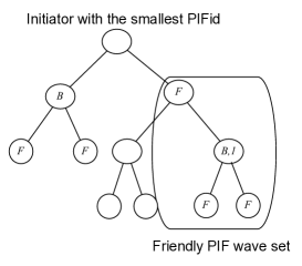
Figure 3: Partial-Final sequence in a $PIF$ Friendly Set

We can state the follow lemma:

Lemma 11

In every $PIF$ friendly set, Partial-Final sequence is reached in finite

Proof

Let consider a single $PIF$ friendly set $S_{i}$. It is clear that if in $S_{i}$ there is only one $PIF$ wave that is executed, then the lemma holds since the $PIF$ wave in $S_{i}$ behaves as the $PIF$ wave described in [8]. In the following we suppose that there are at least two $PIF$ waves that are executed in each $PIF$ friendly set.

Observe that the behavior of $PIF$ waves when they are alone (when they do not meet any other $PIF$ wave) is similar to the well now $PIF$ schema in [8], thus, we will not discuss their progression in this case. Let us consider the $PIF$ wave that has the smallest identifier $id$ in the set $S_{i}$ (let refer to its initiator by $InitTarget$). The cases bellow are then possible:

1. There exists a node $p$ such as $S_{p}=(C,NULL,NULL)$ $\wedge$ $\exists$ $q,q^{\prime}\in N_{p}$, $S_{q}=(B,id,z)$ $\wedge$ $S_{q^{\prime}}=(B,id^{\prime},z^{\prime})$. Note that $id<id^{\prime}$. In this case $p$ sets its state to the broadcast phase and chooses $q$ as its father $S_{p}=(B,id,q)$. Note that for the node $q^{\prime}$ we retrieve case 2.

2. There exists a node $p$ such as $S_{p}=(B,id^{\prime},q)$ $\wedge$ $\exists$ $q^{\prime}\in N_{p}$, $S_{q^{\prime}}=(B,id,z)$ $\wedge$ $z\neq p$. Note that $id<id^{\prime}$. In this case we are sure that $S_{q}=(B,id^{\prime\prime},z)$ with $id^{\prime\prime}\leq id^{\prime}$ and $z\neq p$ (recall that there in no more abnormal sequences). Thus, $p$ changes its state to $S_{p}=(B,id,q^{\prime})$. Note that $p$ was part of path $P_{id^{\prime}}$. From Lemma 10, all the nodes on the path will updates their state as well. Thus the initiator of the $PIF$ wave of identifier $id^{\prime}$ will be able to know that there is another $PIF$ wave with a smaller $id$ that is being executed (let refer to such a node by $Init_{id^{\prime}}$). $Init_{id^{\prime}}$ updates it state to be part of the $PIF$ wave of identifier $id$ (refer to Rule $R5$). Note that only the node that are on the path of both $p$ and $Init_{id^{\prime}}$ updates their state. The other nodes (that were part of $PIF_{id^{\prime}}$) don’t have to update their state since when the nodes of the path update their state, they are already part of $SubTree(p)$.
   Observe that since some of the nodes that are part of $SubTree(p)$ do not change their state, Some $PIF$ waves can be seen as $PIF$ waves with smaller $id$. Refer to Figure 4. (From the figure (case ($c$)) we can observe that $p^{\prime}$ is not aware of the presence of the $PIF$ wave of $id=0$ since it did not change its state). Let $p_{0}$ be the node that is neighbor to the initiator of the $PIF$ wave $PIF1$ that has the smallest $id$. Note that $S_{p_{0}}=(B,id,z)$ ($p$ in Figure 4) and let $p_{k}$ be the node that is neighbor to the initiator of the other $PIF$ (the one that can be considered as the $PIF$ wave with the smallest $id$, the $PIF$ wave with $id=1$ in Figure 4). Observe that $S_{p_{k}}=(B,id^{\prime},z^{\prime})$. Let $P=p_{1},p_{2},p_{3},...p_{k-1}$ be the sequence of nodes between $p_{0}$ and $p_{k}$ such as $S_{p_{i}}=(B,id^{\prime\prime},p_{i-1})$ and $id^{\prime\prime}>id$. Note that on $p_{k-1}$, $R4$ is enabled. When the rule is executed, $p_{k-1}$ updates its state to $S_{p_{k-1}}=(B,id^{\prime},p_{k})$. Note that on $p_{k-2}$, $R4$ becomes enabled thus, $p_{k-2}$ will have the same behavior, it updates its state to $S_{p_{k-2}}=(B,id^{\prime},p_{k-2})$ and so on. Hence, all the nodes on $P$ except $p_{1}$ will updates their state and set it at $(B,id^{\prime},p_{i+1})$. Note that $p_{1}$ is able to detect the presence of the two $PIF$ waves since it has two neighboring nodes that are part of different $PIF$ waves, it is able to detect that $p_{2}$ think that the $PIF$ with the identifier $id^{\prime}$ is the smallest one. Thus, $p_{1}$ updates its state by changing the identifier of the $PIF$ waves to set it at the smallest one. ($S_{p_{1}}=(B,id,z)$). By doing so, $R4$ becomes enabled on $p_{2}$. When the rule is executed, $p_{2}$ updates its state and so on.

Let $p_{init}$ be the node that initiates a $PIF$ wave that has the smallest $id$ within the $PIF$ friendly $S_{i}$. From the two cases above, we can deduce that all the nodes part of the same $S_{i}$ will be part of the $SubTree(p_{init})$. Note that when the feedback phase finished its execution, all the nodes in $S_{i}$ except $p_{init}$ will be in the feedback phase. Thus a Partial-Final configuration is reached and the lemma holds.

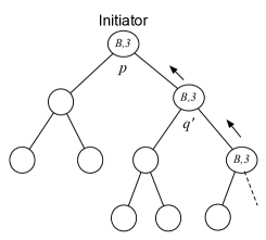
(a) A PIF wave with id=3 is being executed.

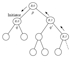
(b) a $PIF$ wave with $id=0$ is initiated. p updates its state.

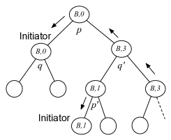
(c) A $PIF$ wave with $id=1$ is initiated. $p^{\prime}$ believe that it is the smallest one and updates its state.

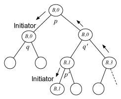
(d) q’ notices the situation and updates the $id_{PIF}$.

Figure 4: Special Case.

From the two cases above, we can deduce that after a finite time, a final-partial configuration is reached in a finite time and the lemma holds.

Lemma 12

Every node belonging to a $PIF$ friendly set eventually clean its state.

Proof

Note that when the configuration of type partial-Final is reached in each set, there is only one node $p$ that is enabled. Observe that $S_{p}=(B,id,NULL)$ (refer to the Rules $R10$ and $R11$). When $p$ executes $R10$, it updates its state to $S_{p}=(C,NULL,NULL)$. Let $N_{1}$ be the set of nodes that are neighbor of $p$. Recursively, let $N_{i}$ be the set of nodes that are neighbor of one node that is part of $N_{i-1}$. Note that $R12$ becomes enabled on all the nodes part of $S1$, when the rule is executed, each node clean its state. In the same manner, $R12$ becomes enabled on the nodes part of $S_{2}$, and so on. Thus we are sure all the nodes part of each $PIF$ friendly set will eventually clean their state and the lemma holds.

From Lemma 12, all the nodes part of $Initial-PIF$ waves clean their state in a finite time. Thus we are sure that a configuration without any $Initial-PIF$ wave is reached in a finite time.

Let us now consider the system at that time (without $Initial-PIF$ waves). In the following we extend the notion of Partial-Final configuration as follow: we say that a configuration is of type Final-Configuration if there exists in the system a single $PIF$ friendly set such that there exists a node $p$ that verifies the following condition: $S_{p}=(B,id,NULL)$ and $\forall$ $q\in S_{i}/\{p\}$, $q\in SubTree(p)$ and $S_{q}=(F,-,-)$

The following lemma follows:

Lemma 13

If there are many $PIF$ waves that are executed then after a finite time, Final Configuration is reached.

Proof

Note that since all the $PIF$ waves that are on the system were initiated by nodes, there is exactly one $PIF$ friendly set i.e., there are no $PIF$ waves that are separated by nodes in the feedback phase (since the Feedback phase is initiated from the leaves of the tree overlay and a node $p$ is allowed to change its to the feedback phase only if all its neighboring nodes except his father are already in the feedback phase). Observe that all the nodes of the system are part of the $PIF$ friendly set. Observe also that the partial-Final configuration in this case is exactly the same as the Final configuration. Thus, we can deduce from Lemma 11 that Final configuration is reached in a finite time. and the lemma holds.

Lemma 14

Starting from a final configuration, all the nodes of the system eventually clean their state.

Proof

Can be deduce directly from Lemma 12 (since Partial-Final configuration is the same as Final configuration when there is a single $PIF$ friendly set in the system). Thus, the lemma holds.

Theorem 4.1

Every node is infinitely often able to initiate a $PIF$ wave

Proof

Directly follows from Lemma 14 and the fact that if Rule $R1$ becomes enabled on $p$, then it remains enabled until $R1$ is executed—$R3$ cannot be enabled while $Request_{PIF}=true$.

We can now state the following result:

Theorem 4.2

Algorithm $1$ is a self-Stabilizing $CoPIF$ algorithm.

Proof

From Theorem 4.1, each node is able to generate a $PIF$ waves in a finite time. From Lemma 13, all the nodes of the system were visited by the $CoPIF$ wave. Thus, all of them acknowledge the receipt of the question (whether the tree overlay is in a correct state or not) and give an answer to the latter. Finally, from Lemma 13 one node $p$ of the system receives the answer ($S_{p}=(B,id,NULL)$). Hence we can deduce that Algorithm $1$ is a self-Stabilizing $CoPIF$ algorithm and the theorem holds.

5 Evaluation

In order to evaluate qualitatively and quantitatively the efficiency of CoPIF, we drive a set of experiments. As mentioned before, the Dlpt approach and its different features have been validated through analysis and simulation [29]. The scalability and performance of its implementation, Sbam (Spades BAsed Middleware) has ever been improved in [9]. Our goal is now to show the efficiency of the previously described QoS algorithm (Section 4). We will focus on the size of the tree, and number of PIF that collaborate simultaneously. We will observe the behavior not only from the number of exchanged messages point of view but also in term of duration needed to performs CoPIFs.

5.1 Sbam

We use the term peer to refer to a physical machine that is available on the network. In our case, a peer is an instantiated Java Virtual Machine connected to other peers through the communication bus. We call nodes the vertices of the prefix tree.

Sbam is the Java implementation of the Dlpt. Sbam proposes $2$-abstraction layers in order to support the distributed data structure: the peer-layer and the agent-layer. The peer-layer is the closest to the hardware layer. It relies on the Ibis Portability Layer (IPL) [17] that enables the P2P communication. We instantiate one JVM per machine, also called peer. JVM communicate all together as a P2P fashion using the IPL communication bus. The agent-layer supports the data structure. Each node of the Dlpt is instantiated as a Sbam agent. Agents are uniformly distributed over peers and communicate together in a transparent way using a proxy interface. Since we want to guarantee truthfulness of information exchanged between Sbam-agents, the implementation of an efficient mechanism ensuring quality of large scale service discovery is quite challenging. In the state model described in the section 3.2 a node has to read the state and the variables of its neighbors. In Sbam, the feature is implemented using synchronous message exchange between agents. Indeed, when a node has to read its neighbor states, it sends a message to each and wait all responses. Despite the fact that this kind of implementation is expensive, especially on a large distributed data structure, experiment (Section 5.6) shown that our model implementation stays efficient, even on a huge prefix tree.

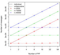
(a) Evolution of number of exchanged messages.

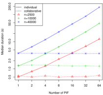
(b) Evolution of duration.

Figure 5: CoPIF behavior

5.2 Experimental platform

Experiments were run on the Grid’5000 platform [7], more precisely on a dedicated cluster HP Proliant DL165 G7 $17$ units, each of them equipped with 2 AMD Opteron 6164 HE (1.7GHz) processors, each processor gathering 12 cores, thus offering a 264-cores platform for these experiments. Each unit consists of 48 GB of memory. Units are connected through two Gigabit Ethernet cards. For each experiment, we deployed one peer per unit.

5.3 Scenario of experiments

The initialization of an experiment works in three phases: ($i$) the communication bus is started on a computing unit (Section 5.2), ($ii$) $16$ peers are launched and connected together through the communication bus, and ($iii$) a pilot is elected using the elect feature of the communication bus.

After the initialization, the pilot drives the experiment. It consists in two sequential steps. First, it sends $n$ insertion requests to the distributed tree structure. An insertion request leads to the addition of a new entry in the Dlpt tree (Section 3). The insertion requests are sent to a random node of the tree and routed following the lexicographic pattern to the targeted node. Doing so, the node sharing the greatest common prefix with the service name is reached. If the targeted label does not exist, a new node is created on a randomly chosen peer and linked to the existing tree.

In the final step, the pilot selects a set of nodes to initiate classic-PIFs and CoPIFs (Section 4). In order to observe distributions, $10$ replications of this basic scenario are executed.

5.4 Failures

At this level of description we can distinguish two kind of failure: ($i$) failures in the Dlpt data structure, when the prefix tree data structure is corrupted; ($ii$) failures in the CoPIF state variables, when state variable dedicated to CoPIF feature are corrupted.

In our experiments, we consider that the Dlpt data structure is not corrupt. It corresponds to the worst case in term of CoPIF truthfulness check. Indeed, if the entire Dlpt data structure is correct, the CoPIF has to explore the entire Dlpt data structure to check it.

Next, remind that the objective of our experiment is to evaluate the efficiency of CoPIF compared to classic-PIF. So, we consider that the CoPIF state variables are not corrupted and we measure the number of messages and the duration of CoPIF when the self-stabilization CoPIF has converged, it means after the clean part of the CoPIF state variables.

5.5 Parameters and indicators

The experiments conducted are influenced by two main parameters. First, $n$ denotes the number of inserted services in the tree. Second, $k$ refers to the number of PIF waves that are collaborating together.

In these experiments, three trees were created with $n$ in the set $\{2500,10000,$
$40000\}$. The number of PIF that collaborate ($k$) was taken from the set $\{1,2,4,8,$
$16,32,64\}$. For each couple $(n,pif)$, $10$ replications are performed. Thus, $210$ experiments were conducted.

Strings used to label the nodes of the trees were randomly generated with an alphabet of $2$ digits and a maximum length of $18$ (in a set of $524287$ key).

For each experiment we observe two indicators: ($i$) the total number of exchanged messages observed and ($ii$) the time required to perform $k$ classic-PIFs or CoPIFs over distributed data structure, i.e., the time between the issue of the PIFs and the receipt of the response on all nodes that initiate PIFs.

For each indicator we obtain $21$ sets of $10$ values. We present evolution of the $median$-value of the $10$-replication according to $k$, the number of PIFs (Figures 5(a) and 5(b)). The comparison of these indicators for classic-PIFs and CoPIFs provides us a qualitative overview of the gain obtain using CoPIF.

In order to quantitatively evaluate the efficiency of the CoPIF strategy, for an indicator ($I$) and for a given number of PIFs $k$, we compute the efficiency criterion with the following formula:

$$E_{I,pif}=\frac{I_{\text{ind},pif}}{pif\times I_{\text{coll},pif}},$$

where $I_{\text{classic},pif}$ (resp. $I_{\text{CoPIF},pif}$) is the value of the indicator $I$ for a given $k$ and in an classic-PIF (resp. CoPIF) context. The evolution of this efficiency criterion are shown in Figures 6(a) and 6(b).

5.6 Results

Figure 5(a) (resp. 5(b)) presents the evolution of the number of messages (resp. duration) needs to execute PIFs according to number of PIFs ($k$) that are simultaneously performed and the size of the data structure on which PIFs are performed. The $y$-axis represents the number of exchanged messages (resp. the duration). On these figures, classic-PIFs and CoPIFs strategies are compared. On both curve, the $x$-axis represents the number of PIF ($k$) that are simultaneously performed. On these figures, we present $2$ curve triplets. Solid (resp. dashed) curves triplet describes indicator in an classic-PIF (resp. CoPIF) context. For each triplet, red-triangle-curve (resp. green-$+$-curve and blue-$x$-curve) describes behavior of indicator for $n=2500$ (resp. $n=10000$ and $n=40000$).

When the indicators explode in for classic-PIF strategy, they stay stable for CoPIF strategy. It qualitatively demonstrates gain of the CoPIF strategy over classic-PIF approach. The introduction of the efficiency criterion in Section 5.5 allows us to measure quantitatively this gain and its behavior.

Figure 6(a) and 6(b) present the efficiency of CoPIF according to the number of exchanged messages and the duration. On these figures we want to observe the impact of the size of the data structure on the efficiency of CoPIF. Figure 6(a) reveals us that, in term of number exchanged messages, on small data structure, the collaborative mechanism is less efficient than on huge one. This result was expected because on small data structure the number of messages due to collision between collaborative PIFs (overhead) represents a more important part of the entire number of exchanged messages. So, the bigger the data structure, the more efficient CoPIF.

More interesting is the analyze of the Figure 6(b). Indeed we can observe the same tendency in term of duration but the efficiency decrease faster with the number of PIFs that are simultaneously performed. It is explain by the fact that overhead messages introduced by CoPIF are particularly expensive messages in term of duration. It quantitatively demonstrates gain of the CoPIF strategy over classic-PIF approach.

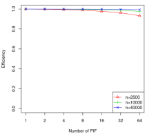
(a) Number of PIF according to the number of exchanged messages.

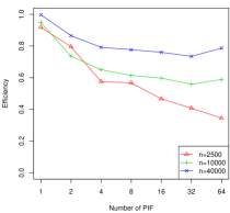
(b) Number of PIF according to the duration.

Figure 6: CoPIF Efficiency

6 Conclusion and Future Work

In this paper we provide a self-stabilized collaborative algorithm called CoPIF allowing to check the truthfulness of a distributed prefix tree. CoPIF implementation in a P2P service discovery framework is experimentally validate, in qualitative and in quantitative terms. Experiment demonstrates the efficiency of CoPIF w.r.t. classic-PIF. CoPIF overhead represents a small part of the number of exchange messages and of the time spend, specially on huge data structures.

We conjecture that the stabilization time is in $O(h^{2})$ rounds and the worst case time to merge several classic-PIF waves is in $O(h)$ rounds, $h$ being the height of the tree. We plan to experimentally validate this two complexities. Indeed, experiment were driven considering no corrupted CoPIF variables. In order to do that, we need to define a model of failure, implement or reuse a fault injector and couple it with Sbam before driving a new experiment campaign.

References

- [1] Karl Aberer, Philippe Cudré-Mauroux, Anwitaman Datta, Zoran Despotovic, Manfred Hauswirth, Magdalena Punceva, and Roman Schmidt. P-grid: a self-organizing structured P2P system. SIGMOD Record, 32(3):29–33, 2003.
- [2] A Arora and MG Gouda. Distributed reset. IEEE Transactions on Computers, 43:1026–1038, 1994.
- [3] J. Aspnes and G. Shah. Skip Graphs. In Fourteenth Annual ACM-SIAM Symposium on Discrete Algorithms, January 2003.
- [4] James Aspnes and Gauri Shah. Skip graphs. ACM Transactions on Algorithms, 3(4), 2007.
- [5] B Awerbuch, S Kutten, Y Mansour, B Patt-Shamir, and G Varghese. Time optimal self-stabilizing synchronization. In STOC93 Proceedings of the 25th Annual ACM Symposium on Theory of Computing, pages 652–661, 1993.
- [6] A. Bharambe, M. Agrawal, and S. Seshan. Mercury: Supporting Scalable Multi-Attribute Range Queries. In Proceedings of the SIGCOMM Symposium, August 2004.
- [7] Raphaël Bolze, Franck Cappello, Eddy Caron, Michel Daydé, Frederic Desprez, Emmanuel Jeannot, Yvon Jégou, Stéphane Lanteri, Julien Leduc, Noredine Melab, Guillaume Mornet, Raymond Namyst, Pascale Primet, Benjamin Quetier, Olivier Richard, El-Ghazali Talbi, and Touché Irena. Grid’5000: a large scale and highly reconfigurable experimental grid testbed. International Journal of High Performance Computing Applications, 20(4):481–494, November 2006.
- [8] Alain Bui, Ajoy Kumar Datta, Franck Petit, and Vincent Villain. Snap-stabilization and PIF in tree networks. Distributed Computing, 20(1):3–19, 2007.
- [9] Eddy Caron, Florent Chuffart, Haiwu He, and Cédric Tedeschi. Implementation and evaluation of a P2P service discovery system. In Proceedings of the the 11th IEEE International Conference on Computer and Information Technology, pages 41–46, 2011.
- [10] Eddy Caron, Ajoy K. Datta, Franck Petit, and Cédric Tedeschi. Self-Stabilization in Tree-Structured Peer-to-Peer Service Discovery Systems. In Proc. of the 27th Int. Symposium on Reliable Distributed Systems (SRDS 2008), Napoli, Italy, October 2008.
- [11] Eddy Caron, Frédéric Desprez, Franck Petit, and Cédric Tedeschi. Snap-stabilizing prefix tree for peer-to-peer systems. Parallel Processing Letters, 20(1):15–30, 2010.
- [12] Eddy Caron, Frédéric Desprez, and Cédric Tedeschi. A Dynamic Prefix Tree for Service Discovery Within Large Scale Grids. In Proc. of the 6th Int. Conference on Peer-to-Peer Computing (P2P’06), pages 106–113, Cambridge, UK, September 2006.
- [13] Eddy Caron, Frédéric Desprez, and Cédric Tedeschi. Efficiency of Tree-Structured Peer-to-Peer Service Discovery Systems. In Proc. of the 5th Int. Workshop on Hot Topics in Peer-to-Peer Systems (Hot-P2P’08), Miami, USA, April 2008.
- [14] Alain Cournier, Ajoy Kumar Datta, Franck Petit, and Vincent Villain. Snap-stabilizing PIF algorithm in arbitrary networks. In 22rd International Conference on Distributed Computing Systems (ICDCS 2002), IEEE Computer Society, pages 199–206, Vienna, Austria, 2002.
- [15] A. Datta, M. Hauswirth, R. John, R. Schmidt, and K. Aberer. Range Queries in Trie-Structured Overlays. In The Fifth IEEE International Conference on Peer-to-Peer Computing, 2005.
- [16] Shlomi Dolev. Self-Stabilization. The MIT Press, 2000.
- [17] Niels Drost, Rob V. van Nieuwpoort, Jason Maassen, Frank Seinstra, and Henri E. Bal. JEL: Unified Resource Tracking for Parallel and Distributed Applications. Concurrency and Computation: Practice and Experience, 2010.
- [18] M. Cai and M. Frank and J. Chen and P. Szekely. Maan: A multi-attribute addressable network for grid information services. Journal of Grid Computing, 2(1):3–14, March 2004.
- [19] P. Maymounkov and D. Mazieres. Kademlia: A Peer-to-Peer Information System Based on the XOR Metric. In Proceedings of IPTPS02, Cambridge, USA, March 2002.
- [20] Elena Meshkova, Janne Riihijärvi, Marina Petrova, and Petri Mähönen. A survey on resource discovery mechanisms, peer-to-peer and service discovery frameworks. Comput. Netw., 52(11):2097–2128, 2008.
- [21] Donald R. Morrison. PATRICIA–Practical Algorithm To Retrieve Information Coded in Alphanumeric. J. ACM, 15:514–534, October 1968.
- [22] S. Ramabhadran, S. Ratnasamy, J. M. Hellerstein, and S. Shenker. Prefix Hash Tree: an Indexing Data Structure over Distributed Hash Tables. In Proceedings of the 23rd ACM Symposium on Principles of Distributed Computing, 2004.
- [23] Sriram Ramabhadran, Sylvia Ratnasamy, Joseph Hellerstein, and Scott Shenker. Prefix hash tree: an indexing data structure over distributed hash table. In Proc. of the 23rd ACM Symposium on Principles of Distributed Computing (PODC’04), page 368, St John’s, Canada, July 2004.
- [24] S. Ratnasamy, P. Francis, M. Handley, R. Karp, and S. Shenker. A Scalable Content-Adressable Network. In ACM SIGCOMM, 2001.
- [25] A. Rowstron and P. Druschel. Pastry: Scalable, Distributed Object Location and Routing for Large-Scale Peer-To-Peer Systems. In International Conference on Distributed Systems Platforms (Middleware), November 2001.
- [26] C. Schmidt and M. Parashar. Enabling Flexible Queries with Guarantees in P2P Systems. IEEE Internet Computing, 8(3):19–26, 2004.
- [27] Y. Shu, B. C. Ooi, K. Tan, and A. Zhou. Supporting Multi-Dimensional Range Queries in Peer-to-Peer Systems. In Peer-to-Peer Computing, pages 173–180, 2005.
- [28] I. Stoica, R. Morris, D. Karger, M. Kaashoek, and H. Balakrishnan. Chord: A Scalable Peer-to-Peer Lookup service for Internet Applications. In ACM SIGCOMM, pages 149–160, 2001.
- [29] Cédric Tedeschi. Peer-to-Peer Prefix Tree for Large Scale Service Discovery. PhD thesis, École normale supérieure de Lyon, October 2008.
- [30] G Varghese. Self-stabilization by counter flushing. In PODC94 Proceedings of the Thirteenth Annual ACM Symposium on Principles of Distributed Computing, pages 244–253, 1994.