Advances on Matroid Secretary Problems:
Free Order Model and Laminar Case

Abstract

The most important open conjecture in the context of the matroid secretary problem claims the existence of an $O(1)$-competitive algorithm applicable to any matroid. Whereas this conjecture remains open, modified forms of it have been shown to be true, when assuming that the assignment of weights to the secretaries is not adversarial but uniformly at random [25, 22]. However, so far, no variant of the matroid secretary problem with adversarial weight assignment is known that admits an $O(1)$-competitive algorithm. We address this point by presenting a $4$-competitive procedure for the free order model, a model suggested shortly after the introduction of the matroid secretary problem, and for which no $O(1)$-competitive algorithm was known so far. The free order model is a relaxed version of the original matroid secretary problem, with the only difference that one can choose the order in which secretaries are interviewed.

Furthermore, we consider the classical matroid secretary problem for the special case of laminar matroids. Only recently, an $O(1)$-competitive algorithm has been found for this case, using a clever but rather involved method and analysis [13] that leads to a competitive ratio of $16000/3$. This is arguably one of the most involved special cases of the matroid secretary problem for which an $O(1)$-competitive algorithm is known. We present a considerably simpler and stronger $3\sqrt{3}e\approx 14.12$-competitive procedure, based on reducing the problem to a matroid secretary problem on a partition matroid. Furthermore, our procedure is order-oblivious, which, as shown in [1], allows for transforming it into a $3\sqrt{3}e$-competitive algorithm for single-sample prophet inequalities.

1 Introduction

The secretary problem is a classical online selection problem of unclear origin [7, 9, 10, 11, 19]. In its original form, the task is to choose the best out of $n$ secretaries, also called elements or items. Secretaries arrive (or are interviewed) one by one in random order. As soon as a secretary arrives, she can be ranked against all previously seen secretaries. Then, before the next one arrives, one has to decide irrevocably whether to choose the current secretary or not. There is a classical algorithm that selects the best secretary with probability $1/e$ [7], and this is known to be asymptotically optimal. In its initial form, the secretary problem was essentially a stopping time problem, and not surprisingly, it mainly attracted the interest of probabilists.

Recently, secretary problems enjoyed a revival, and various generalizations have been studied. These developments are strongly motivated by a close connection to online mechanism design, where a good is sold to agents arriving online [16, 2]. Here, the agents correspond to the secretaries and they reveal prices that they are willing to pay in exchange for goods. This leads to secretary problems where more than one secretary can be chosen. The most canonical generalization asks to hire $k$ out of $n$ secretaries, each revealing a non-negative weight upon arrival, and the goal is to hire a maximum weight subset of $k$ secretaries. This interesting variant was introduced and studied by Kleinberg [16], who presented a $(1-O(1/\sqrt{k}))$-competitive algorithm for this setting. However, in many applications, additional constraints have to be imposed on the elements that can be chosen. A very general class of constrained secretary problems, where the chosen elements have to form an independent set of a given matroid $M=(N,\mathcal{I})$, was introduced by Babaioff, Immorlica and Kleinberg [2]. This setting, now generally termed matroid secretary problem, covers at the same time many interesting cases and has a rich structure that can be exploited to design algorithms with strong competitive ratios.

To give a concrete example of a matroid secretary problem, and to motivate some of our results, consider the following connection problem. Given is an undirected graph $G=(V,E)$, representing a communication network, with non-negative edge-capacities $c:E\rightarrow\mathbb{Z}_{\geq 0}$ and a server $r\in V$. Clients, which are the equivalent of candidates in the secretary problem, reside at vertices of the graph and are interested in being connected to the server $r$ via a unit-capacity path. The number of clients and their locations are known. Each client has a price that she is willing to pay to connect to the server. These prices are unknown and no assumptions are made on them except for being non-negative. Clients then reveal themselves one by one in random order, announcing their price. Whenever a client reveals herself, the network operator has to decide irrevocably before the next client appears whether to serve this client and receive the announced price. The goal is to choose a maximum weight subset of clients that can be served simultaneously without exceeding the given capacities $c$. It is well-known that the constraints imposed by the limited capacity on the clients that can be chosen is a special type of matroid constraint, namely a gammoid constraint [23].

For the classical matroid secretary problem, as discussed above, the currently asymptotically best competitive algorithm is an $O(\sqrt{\log{\rho}})$-competitive method by Chakraborty and Lachish [4], where $\rho$ is the rank of the matroid. This improved on an earlier $O(\log{\rho})$-competitive algorithm of Babaioff, Immorlica and Kleinberg [2]. Babaioff et al. [2] asked about the existence of an $O(1)$-competitive algorithm for the matroid secretary problem. This question remains open and is arguably the currently most important open question regarding the matroid secretary problem.

Motivated by this conjecture, many interesting advances have been made to obtain $O(1)$-competitive methods, either for special cases of the matroid secretary problem or variants thereof. In particular, $O(1)$-competitive algorithms have been found for graphic matroids [2, 18] (currently best competitive ratio: $2e$), transversal matroids [2, 5, 18] ($8$-competitive), co-graphic matroids [25] ($3e$-competitive), linear matroids with at most $k$ non-zero entries per column [25] ($ke$-competitive), laminar matroids [13] ($16000/3$-competitive), regular matroids ($9e$-competitive) [6], and some types of decomposable matroids, including max-flow min-cut matroids [6] ($9e$-competitive). For most of the above special cases, strong competitive algorithms have been found, typically based on very elegant techniques. However for the laminar matroid, only a considerably higher competitive ratio is known due to Im and Wang [13], using a very clever but quite involved method and analysis.

Furthermore, variants of the matroid secretary problem have been investigated that assume random instead of adversarial assignment of the weights, and for which $O(1)$-competitive algorithms can be obtained without any restriction on the underlying matroid. Recall that the classical matroid secretary problem does not make any assumptions on how weights are assigned to the elements, which means that we have to assume a worst-case, i.e., adversarial, weight assignment. However, the order in which the elements reveal themselves is assumed to be random. Soto [25] considered the variant where not only the arrival order of the elements is assumed to be uniformly random but also the assignment of the weights to the elements, and presented a $5.7187$-competitive algorithm for this case. More precisely, in this model, the weights can still be chosen by an adversary, but are then assigned uniformly at random to the elements of the matroid. Building upon earlier work of Soto [24], Vondrák and Oveis Gharan [22] showed that a $40e/(e-1)$-competitive algorithm can even be obtained when the arrival order of the elements is adversarial and the assignment of weights remains uniformly at random. This was later improved to a $16e/(e-1)$-competitive algorithm by Soto [25]. Hence, this model is somehow the opposite of the classical matroid secretary problem, where assignment is adversarial and arrival order is random.

However, so far, no progress has been made in variants with adversarial assignment. One such variant, suggested shortly after the introduction of the matroid secretary problem [17], assumes that the appearance order of elements can be chosen by the algorithm. More precisely, in this model, which we call the free order model, whenever a next element has to reveal itself, the algorithm can choose the element to be revealed. For example, in the above network connection problem, one could decide at each step which is the next client to reveal its price, by using for this decision the network structure and the elements observed so far. A main further complication when dealing with adversarial assignments—as in the free order model—contrary to random assignment, is that the knowledge of the initial structure of the matroid seems to be of little help. This is due to the fact that an adversary can assign a weight of zero to most elements of the matroid, and only give a non-negative weight to a selected subset $A\subseteq N$ of elements. Hence, the problem essentially reduces to the restriction $M|_{A}$ of the matroid $M$ over the elements $A$. However, the structure of $M|_{A}$ is essentially impossible to guess from $M$. This is in stark contrast to models with random assignment, e.g., in the model considered by Soto, the mentioned $2e^{2}/(e-1)$-competitive algorithm exploits the given structure of the matroid $M$, by partitioning $N$ and solving a standard single secretary problem on each part of the partition. Different approaches are needed for adversarial weight assignments.

In this paper we are interested in the following two questions. First, is there an $O(1)$-competitive algorithm for the free order model? Second, can we get a better understanding of the laminar case of the classical secretary problem, with the goal to find considerably stronger and simpler procedures?

As is common in this context, we use competitive analysis to judge the quality of algorithms. More precisely, an algorithm is $c$-competitive if it returns a (random) solution whose expected value is at least $\frac{1}{c}\operatorname{OPT}$, where $\operatorname{OPT}$ is the value of an offline optimum solution, i.e., a maximum weight independent set. Hence, the goal is to find $c$-competitive algorithms with $c\geq 1$ being as close as possible to $1$.

Our results and techniques

We present a $4$-competitive algorithm for the free order model, thus obtaining the first $O(1)$-competitive algorithm for a variant of the matroid secretary problem with adversarial weight assignment, without any restriction on the underlying matroid. This algorithm is in particular applicable to the previously mentioned network connection problem, when the order, in which the network operator negotiates with the clients, can be chosen.

On a high level, our algorithm follows a quite intuitive idea, which, interestingly, does not work in the traditional matroid secretary problem. In a first phase, we draw each element with probability $0.5$ to obtain a set $A\subseteq N$, without selecting any element of $A$. Let $\operatorname{OPT}_{A}$ be the best offline solution in $A$. We call an element $f\in N\setminus A$ good, if it can be used to improve $\operatorname{OPT}_{A}$, in the sense that either $\operatorname{OPT}_{A}\cup\{f\}$ is independent or there is an element $g\in\operatorname{OPT}_{A}$ such that $(\operatorname{OPT}_{A}\setminus\{g\})\cup\{f\}$ is independent and has a higher value than $\operatorname{OPT}_{A}$. In the second phase, we go through the remaining elements $N\setminus A$, drawing element by element in a well-chosen way to be specified soon. We accept an element $f\in N\setminus A$ if it is good and does not destroy independence when added to the elements accepted so far. Our approach fails if elements are drawn randomly in the second phase. The main problem when drawing randomly, is that we may accept good elements of relatively low value that may later block some high-valued good elements, in the sense that they cannot be added anymore without destroying independence of the selected elements. To overcome this problem, we determine after the first phase a specific order of how elements will be drawn in the second phase. The idea is to first draw elements of $N\setminus A$ that are in the span of elements of $A$ of high weight. More precisely, let $A=\{a_{1},\dots,a_{m}\}$ be the numbering of the elements of $A$ according to decreasing weights. In the second phase we start by drawing elements of $(N\setminus A)\cap\operatorname{span}(\{a_{1}\})$, then $(N\setminus A)\cap\operatorname{span}(\{a_{1},a_{2}\})$, and so on. One particular situation, where the above ordering becomes very intuitive, is if there is a set $S\subseteq N$ with a high density of high-valued elements. In this case it is likely that many elements of $S$ are part of $A$. Hence, high-valued elements of $A$ span further high-valued elements in $S$. Thus, by the above order, we are likely to draw high-valued elements of $S$ early, before they can be blocked by the inclusion of lower-valued elements.

Similar to previous secretary algorithms, we show that our algorithm is $O(1)$-competitive by proving that each element $f\in\operatorname{OPT}$ of the global offline optimum $\operatorname{OPT}$ will be chosen with probability at least $1/4$. However, the way we prove this is based on a novel approach. Broadly speaking, we show that an element $f\in\operatorname{OPT}$ gets selected if additionally to $f\not\in A$, the following property holds: either $f\not\in\operatorname{span}((N\setminus A)\setminus\{f\})$, or the maximum value $\beta\geq 0$ such that $f$ is spanned by elements in $(N\setminus A)\setminus\{f\}$ of weight $\geq\beta$ is smaller than the maximum value $\alpha\geq 0$ such that $f$ is spanned by elements in $N\cap A$ of weight $\geq\alpha$. Exploiting that the distributions of $A$ and $N\setminus A$ are identical, we show that the above conditions happens with probability at least $1/4$.

In an earlier short version of this paper [14], we only proved that our algorithm is $9$-competitive. Our proof was later refined and simplified by Azar, Kleinberg and Weinberg [1] to show $4$-competitiveness of our procedure. Due to this recent development, we present here the refined analysis of [1]. We are thankful to the authors of [1] for their agreement to include this analysis in the present paper.

Furthermore, we present a new approach to deal with laminar matroids in the classical matroid secretary model. Our technique leads to a $3\sqrt{3}e\approx 14.12$-competitive procedure, thus considerably improving on the $16000/3\approx 5333$-competitive algorithm of Im and Wang [13]. Our main contribution here is to present a simple way to transform the matroid secretary problem on a laminar matroid $M$ to one on a unitary partition matroid $M_{P}$ by losing only a small constant factor of $3\sqrt{3}\approx 5.2$. The secretary problem on $M_{P}$ can then simply be solved by applying the classical $e$-competitive algorithm for the standard secretary problem to each partition of $M_{P}$. We first observe a constant fraction of all elements, on the basis of which a partition matroid $M_{P}$ on the remaining elements is then constructed. To assure feasibility, $M_{P}$ is defined such that each independent set of $M_{P}$ is also an independent set of $M$. To best convey the main ideas of our procedure, we first present a very simple method to obtain a weaker $27e/2\approx 36.7$-competitive algorithm, which already improves considerably on the $16000/3$-competitive algorithm of Im and Wang. The $3\sqrt{3}e$-competitive algorithm is then obtained through a strengthening of this approach by using a stronger partition matroid $M_{P}$ and a tighter analysis.

A further advantage of our procedure for laminar matroids is the fact that it leads to $O(1)$-competitive algorithms in the context of single-sample matroid prophet inequalities, which in turn implies strong algorithms for order-oblivious posted pricing mechanisms, as shown by Azar, Kleinberg and Weinberg [1]. More precisely, prophet inequalities are a setting that is closely related to the matroid secretary problem. The key difference is that the weight of each element comes from a distribution that depends on the element, and depending on the setting may or may not be known in advance. In single-sample prophet inequalities, one only knows a single sample from each distribution, and the order in which the elements arrive is adversarial, which is another key difference to the classical matroid secretary problem. It was shown in [1] that an $\alpha$-competitive matroid secretary algorithm can be transformed into an $\alpha$-competitive algorithm for single-sample prophet inequalities, if the secretary algorithm is order-oblivious. Loosely speaking, an order-oblivious procedure is one that consists of two phases, where in a first phase a subset of the elements is observed without choosing any element, and furthermore, the competitive ratio does not dependent on the order in which elements appear in the second phase. Hence, the algorithm does not need the random order assumption during the second phase. Contrary to the previous $O(1)$-competitive laminar secretary algorithm [13], and also a subsequently introduced $O(1)$-competitive algorithm for this case [21], our algorithm is order-oblivious. We refer the reader to [1] for more information on order-oblivious algorithms and single-sample prophet inequalities. Furthermore, [1] also discusses the implications of our algorithm for laminar matroids in this context.

We remark that the algorithms we present do not need to observe the exact weights of the items when they reveal themselves, but only need to be able to compare the weights of elements observed so far. This is a common feature of many matroid secretary algorithms and matroid algorithms more generally.

To simplify the exposition, we assume that all weights are distinct, i.e., they induce a linear order on the elements. This implies in particular, that there is a unique maximum weight independent set. The general case with possibly equal weights easily reduces to this case by breaking ties arbitrarily between elements of equal weight, to obtain a linear order.

Related work

Recently, matroid secretary problems with submodular objective functions have been considered. For this setting, $O(1)$-competitive procedures have been found for knapsack constraints, uniform matroids, and, if the submodular objective is furthermore monotone, for partition matroids, and more generally for intersections of laminar matroids, and transversal matroids (see [3, 8, 12, 21]).

Additionally, variations of the matroid secretary problem have been studied with restricted knowledge on the underlying matroid type. This includes the case where no prior knowledge of the underlying matroid is assumed except for the size of the ground set. Or even more extremely, the case without even knowing the size of the ground set. For more information on such variations we refer to the excellent overview in [22].

Subsequent results

We would like to highlight that very recently, after a previous version [15] of this article, Ma, Tang and Wang [20, 21] further improved the competitive ratio for the secretary problem on laminar matroids by presenting a $9.6$-competitive algorithm. They use an interesting and natural algorithmic idea, including elements only if they are part of the offline optimum of all elements seen so far. The description of their algorithm is nice and elegant, however, its analysis is somewhat involved. Unfortunately, their algorithm is not order-oblivious and therefore cannot be used in the context of single-sample prophet inequalities.

Organization of the paper

Our $4$-competitive algorithm for the free order model is presented in Section 2. Section 3 discusses our algorithms for the classical matroid secretary problem. We start by presenting in Section 3.1 our simple $27e/2$-competitive method, and then show in Section 3.2 how to strengthen the algorithm and its analysis to obtain the claimed $3\sqrt{3}e$-competitiveness.

2 A $4$-competitive algorithm for the free order model

To simplify the writing we use “$+$” and “$-$” for the addition and subtraction of single elements from a set, i.e., $S+f-g=(S\cup\{f\})\setminus\{g\}$. Furthermore, for $k\in\mathbb{Z}_{\geq 1}$ we use the shorthand $[k]:=\{1,\dots,k\}$. Algorithm 1 describes our $4$-competitive algorithm for the free order model.

Algorithm 1 A $4$-competitive algorithm for the free order model.

1. Draw each element with probability $0.5$ to obtain $A\subseteq N$, without selecting any element of $A$. We number the elements of $A=\{a_{1},\dots,a_{m}\}$ in decreasing order of weights. Define $A_{i}=\{a_{1},\dots,a_{i}\}$, with $A_{0}=\emptyset$.
   Initialize: $I\leftarrow\emptyset$.

2. For $i=1$ to $m$:
       draw one by one (in any order) all elements $f\in(\operatorname{span}(A_{i})\setminus\operatorname{span}(A_{i-1}))\setminus A$:
          if $I+f\in\mathcal{I}$ and $\mathrm{w}(f)>\mathrm{w}(a_{i})$, then $I=I+f$.
   For all remaining elements $f\in N\setminus\operatorname{span}(A)$ (drawn in any order):
       if $I+f\in\mathcal{I}$, then $I=I+f$.
   Return $I$

To analyze Algorithm 1, we introduce some additional notation. Let $\{e_{1},\dots,e_{n}\}=N$ be the numbering of the elements of the ground set satisfying $\mathrm{w}(e_{1})>\dots>\mathrm{w}(e_{n})$. Furthermore, for each $j\in[n]$, we define $N_{j}:=\{e_{1},\dots,e_{j}\}$.

As mentioned previously, a good element $f\in N\setminus A$ is an element that allows for improving the maximum weight independent set in $A$, i.e., the unique maximum weight independent set in $A+f$ includes $f$. An element $f$ being good thus means that it gets selected when applying the greedy algorithm to $A+f$. Hence, $f$ is good if and only if $f\not\in\operatorname{span}(\{a\in A\mid\mathrm{w}(a)>\mathrm{w}(f)\})$, which can be rephrased as $f$ is good if either $f\not\in\operatorname{span}(A)$, or if there is an index $i\in[m]$ such that $f\in\operatorname{span}(A_{i})\setminus\operatorname{span}(A_{i-1})$ and $\mathrm{w}(f)>\mathrm{w}(a_{i})$. Hence, our algorithm indeed only accepts good elements. Furthermore, whenever any element $f$ of the offline optimum $\operatorname{OPT}$ is considered in some iteration $i\in[m]$ in the first for-loop of step 2—i.e., $f\in(\operatorname{span}(A_{i})\setminus\operatorname{span}(A_{i-1}))\setminus A$—then we always have $\mathrm{w}(f)>\mathrm{w}(a_{i})$. Hence, an element $f\in\operatorname{OPT}$ gets selected by Algorithm 1 if and only if $I+f\in\mathcal{I}$, where $I$ is the set of already selected elements at the time when $f$ is considered.

To show that Algorithm 1 is $4$-competitive, we show that each element $f\in\operatorname{OPT}$ will be contained in the set $I$ returned by the algorithm with probability at least $1/4$. Hence, let $f\in\operatorname{OPT}$, and define

$$j_{1} :=\operatorname{argmin}\{j\in[n]\mid f\in\operatorname{span}((N_{j}\cap A)-f)\},$$

$$j_{2} :=\operatorname{argmin}\{j\in[n]\mid f\in\operatorname{span}((N_{j}\setminus A)-f)\},$$

where, if $f\not\in\operatorname{span}(A-f)$ we set $j_{1}=\infty$, and and $f\not\in\operatorname{span}((N\setminus A)-f)$ then $j_{2}=\infty$. Notice that both $j_{1}$ and $j_{2}$ are random variables that depend on the random set $A$. The following lemma provides a simple property under which $f$ gets selected.

Lemma 1.

If $j_{1}\leq j_{2}$ and $f\not\in A$ then $f$ gets selected by Algorithm 1.

Proof.

We first handle the case $j_{2}=\infty$. Consider the moment when $f$ is considered in the second step of Algorithm 2, either in the first or second for-loop, and let $I$ be the elements selected so far by the algorithm. As discussed above, since $f\in\operatorname{OPT}$, we only have to show $I+f\in\mathcal{I}$ for $f$ to be selected, which holds because

$$f\overset{j_{2}=\infty}{\not\in}\operatorname{span}((N\setminus A)-f)\overset{I\subseteq(N\setminus A)-f}{\supseteq}\operatorname{span}(I),$$

and hence, $f\not\in\operatorname{span}(I)$.

Now assume $j_{2}<\infty$, and therefore also $j_{1}<\infty$ since $j_{1}\leq j_{2}$. Consider the moment when $f$ is considered in the second step of Algorithm 1, and let $I$ be the set of elements selected so far by the algorithm. Notice that since $j_{1}<\infty$, we have $f\in\operatorname{span}(A-f)$, and therefore, $f$ is considered at some iteration $i\in[m]$ during the first for-loop of step 2 of the algorithm. Furthermore, $i$ is the smallest index in $[m]$ such that $f\in\operatorname{span}(A_{i})$, and thus, $a_{i}=e_{j_{1}}$. Hence, $I$ only contains elements of weight strictly larger than $\mathrm{w}(e_{j_{1}})$, i.e., $I\subseteq N_{j_{1}-1}$. Furthermore, since $I\subseteq N\setminus A$, this implies $I\subseteq N_{j_{1}-1}\setminus A$. Again we have $I+f\in\mathcal{I}$ since

$$f\overset{\text{def.~{}of $j_{2}$}}{\not\in}\operatorname{span}((N_{j_{2}-1}\setminus A)-f)\overset{j_{1}\leq j_{2}}{\supseteq}\operatorname{span}((N_{j_{1}-1}\setminus A)-f)\overset{I\subseteq(N_{j_{1}-1}\setminus A)-f}{\supseteq}\operatorname{span}(I).$$

∎

Leveraging Lemma 1, we can now prove the correctness of the algorithm by showing that $j_{1}\leq j_{2}$ with probability at least $0.5$.

Theorem 2.

Algorithm 1 selects each element $f\in\operatorname{OPT}$ with probability at least $1/4$, and is therefore $4$-competitive.

Proof.

The key observation is that for every $S\subseteq N$, either $j_{1}\leq j_{2}$ for $A=S$ or $j_{1}\leq j_{2}$ for $A=N\setminus S$. Since the two events $A=S$ and $A=N\setminus S$ occur with the same probability, we obtain $\Pr[j_{1}\leq j_{2}]\geq 0.5$. Furthermore, whether $f\in A$ or not is independent of the two random variables $j_{1}$ and $j_{2}$. Thus,

$$\Pr[f\not\in A\text{ and }j_{1}\leq j_{2}]=\Pr[f\not\in A]\cdot\Pr[j_{1}\leq j_{2}]\geq\frac{1}{2}\cdot\frac{1}{2}=\frac{1}{4},$$

and by Lemma 1, the probability of $f$ being selected by Algorithm 1 is at least $1/4$. ∎

3 Classical secretary problem for laminar matroids

Let $M=(N,\mathcal{I})$ be a laminar matroid whose constraints are defined by the laminar family $\mathcal{L}\subseteq 2^{N}$ with upper bounds $b_{L}$ for $L\in\mathcal{L}$ on the number of elements that can be chosen from $\mathcal{L}$, i.e., $\mathcal{I}=\{I\subseteq N\mid|I\cap L|\leq b_{L}\;\forall L\in\mathcal{L}\}$. Without loss of generality we assume $b_{L}\geq 1$ for $L\in\mathcal{L}$, since otherwise we can simply remove all elements of $L$ from $M$. Furthermore, we assume $N\in\mathcal{L}$, since otherwise a redundant constraint $|I\cap N|\leq b_{N}$ can be added by choosing a sufficiently large right-hand side $b_{N}$.

3.1 A simple $27e/2$-competitive algorithm for the laminar secretary problem

To reduce the matroid secretary problem on $M$ to a problem on a partition matroid, we first number the elements $N=\{f_{1},\dots,f_{n}\}$ such that for any set $L\in\mathcal{L}$, the elements in $L$ are numbered consecutively, i.e., $L=\{f_{p},\dots,f_{q}\}$ for some $1\leq p<q\leq n$. Figure 1 shows an example of such a numbering.

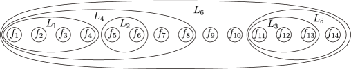
Figure 1: An example of a numbering of the elements of the ground set such that each set $L\in\mathcal{L}=\{L_{1},\dots,L_{6}\}$ of the laminar family contains consecutively numbered elements.

For the sake of exposition, we start by presenting a conceptually simple algorithm and analysis, based on the introduced numbering of the ground set, that leads to a competitive ratio of $27e/2$. The claimed $3\sqrt{3}e$-competitive algorithm follows the same ideas, but strengthens both the approach and analysis. Algorithm 2 describes our $27e/2$-competitive procedure.

Algorithm 2 A $27e/2$-competitive algorithm for laminar matroids.

1. Observe $\operatorname{Binom}(n,2/3)$ elements of $N$, which we denote by $A\subseteq N$.
   Determine maximum weight independent set $\operatorname{OPT}_{A}=\{f_{i_{1}},\dots,f_{i_{p}}\}$ in $A$ where $1\leq i_{1}<\dots<i_{p}\leq n$. Define $P_{j}=\{f_{k}\mid k\in\{i_{j-1},\dots,i_{j}\}\}\setminus A$ for $j\in\{1,\dots,p+1\}$, where we set $i_{0}=0,i_{p+1}=n$. Let

   $$\mathcal{P}_{\operatorname{odd}}(A) =\{P_{j}\mid j\in[p+1],j\text{ odd}\},$$

   $$\mathcal{P}_{\operatorname{even}}(A) =\{P_{j}\mid j\in[p+1],j\text{ even}\}.$$

   If $\operatorname{OPT}_{A}=\emptyset$ then set $\mathcal{P}=\{N\setminus A\}$,
   else set $\mathcal{P}=\mathcal{P}_{\operatorname{odd}}(A)$ with probability $0.5$, otherwise set $\mathcal{P}=\mathcal{P}_{\operatorname{even}}(A)$.

2. Apply to each set $P\in\mathcal{P}$ an $e$-competitive classical secretary algorithm to obtain an element $g_{P}\in P$.
   Return $\{g_{P}\mid P\in\mathcal{P}\}$.

Notice that applying a standard secretary algorithm to the sets of $\mathcal{P}$ in step 2 can easily be performed by running $|\mathcal{P}|$ many $e$-competitive secretary algorithms in parallel, one for each set $P\in\mathcal{P}$. Elements are drawn one by one in the second phase, and they are forwarded to the secretary algorithm corresponding to the set $P$ that contains the drawn element, and are discarded if no set of $\mathcal{P}$ contains the element. Furthermore, observe that $A$ contains each element of $N$ independently with probability $2/3$.

We start by observing that Algorithm 2 returns an independent set.

Lemma 3.

Let $A\subseteq N$ with $\operatorname{OPT}_{A}\neq\emptyset$ and let $\mathcal{P}\in\{\mathcal{P}_{\operatorname{even}}(A),\mathcal{P}_{\operatorname{odd}}(A)\}$. For each $P\in\mathcal{P}$, let $g_{p}$ be any element in $P$. Then $\{g_{P}\mid P\in\mathcal{P}\}\in\mathcal{I}$.

Proof.

Let $I=\{g_{P}\mid P\in\mathcal{P}\}$ be a set as stated in the lemma. Notice that for any two elements $f_{k},f_{\ell}\in I$ with $k<\ell$ we have $|\operatorname{OPT}_{A}\cap\{f_{k},f_{k+1},\dots,f_{\ell}\}|\geq 2$. Now consider a set $L\in\mathcal{L}$ corresponding to one of the constraints of the underlying laminar matroid. By the above observation and since $L$ is consecutively numbered, at least one of the following holds: (i) $|L\cap I|=1$, or (ii) $|L\cap\operatorname{OPT}_{A}|\geq|L\cap I|$. If case (i) holds, then the constraint corresponding to $L$ is not violated since we assumed $b_{L}\geq 1$. If (ii) holds, then $L$ is also not violated since $|L\cap I|\leq|L\cap\operatorname{OPT}_{A}|\leq b_{T}$ because $\operatorname{OPT}_{A}\in\mathcal{I}$. Hence $I\in\mathcal{I}$. ∎

Theorem 4.

Algorithm 2 is $27e/2$-competitive for the laminar matroid secretary problem.

Proof.

Let $\operatorname{OPT}\in\mathcal{I}$ be the maximum weight independent set in $N$, i.e., the offline optimum. Furthermore, let $I$ be the set returned by Algorithm 2, and let $f\in\operatorname{OPT}$. We say that $f$ is solitary if $\exists\>P\in\mathcal{P}$ with $P\cap\operatorname{OPT}=\{f\}$. Similarly we call $P\in\mathcal{P}$ solitary if $|P\cap\operatorname{OPT}|=1$. We prove the theorem by showing that each element $f\in\operatorname{OPT}$ is solitary with probability $\geq 2/27$. This indeed implies the theorem since we can do the following type of accounting. Let $X_{f}$ be the random variable which is zero if $f$ is not solitary, and otherwise equals the weight of the element $g\in I$ that was chosen by the algorithm from the set $P$ that contains $f$. By only considering the weights of elements chosen in solitary sets $\mathcal{P}$ we obtain

$${\bf E}[w(I)]\geq\sum_{f\in\operatorname{OPT}}{\bf E}[X_{f}].$$ (1)

However, if each element $f\in\operatorname{OPT}$ is solitary with probability $2/27$, we obtain ${\bf E}[X_{f}]\geq\frac{2w(f)}{27e}$, because the classical secretary algorithm will choose with probability $1/e$ the maximum weight element of the set $P$ that contains the solitary element $f$. Combining this with (1) yields ${\bf E}[w(I)]\geq\frac{2}{27e}w(\operatorname{OPT})$ as desired. Let us then show that each $f\in\operatorname{OPT}$ is solitary with probability $\geq 2/27$.

Let $f_{i}\in\operatorname{OPT}$. We assume that $\operatorname{OPT}$ contains an element with a lower index than $i$ and one with a higher index than $i$. The cases of $f_{i}$ being the element with highest or lowest index in $\operatorname{OPT}$ follow analogously. Let $f_{j}\in\operatorname{OPT}$ by the element of $\operatorname{OPT}$ with the largest index $j<i$. Similarly, let $f_{k}\in\operatorname{OPT}$ be the element of $\operatorname{OPT}$ with the smallest index $k>i$. One well-known matroidal property that we use is $\operatorname{OPT}\cap A\subseteq\operatorname{OPT}_{A}$. Hence, if $f_{j},f_{k}\in A$ then $f_{j},f_{k}\in\operatorname{OPT}_{A}$, and if furthermore $f_{i}\not\in A$, then $f_{i}$ will be the only element of $\operatorname{OPT}$ in the set $P\in\mathcal{P}_{\operatorname{odd}}(A)\cup\mathcal{P}_{\operatorname{even}}(A)$ that contains $f_{i}$. Hence, if the coin flip in Algorithm 2 chooses the family $\mathcal{P}\in\{\mathcal{P}_{\operatorname{odd}}(A),\mathcal{P}_{\operatorname{even}}(A)\}$ that contains $P$, then $f_{i}$ is solitary. To summarize, $f_{i}$ is solitary if $f_{j},f_{k}\in A$, $f_{i}\not\in A$ and the coin flip for $\mathcal{P}$ turns out right. This happens with probability $\left(\frac{2}{3}\right)^{2}\cdot\left(1-\frac{2}{3}\right)\cdot\frac{1}{2}=\frac{2}{27}$. ∎

3.2 A $3\sqrt{3}e$-competitive algorithm for the laminar matroid secretary problem

One conservative aspect of the proof of Theorem 4 is that we only consider the contribution of solitary elements. Additionally, a drawback of Algorithm 2 itself is that about half of the elements of $N\setminus A$ are ignored as we only select from either $\mathcal{P}_{\operatorname{odd}}(A)$ or $\mathcal{P}_{\operatorname{even}}(A)$. In this section, we address these two weaknesses to obtain a $3\sqrt{3}e$-competitive algorithm.

We start by describing a stronger way to define a partition $\mathcal{P}$ of $N\setminus A$ and reduce the problem to a matroid secretary problem on the unitary partition matroid defined on $\mathcal{P}$.

For any independent set $I\in\mathcal{I}$, we define a partition $\widetilde{\mathcal{P}}(I)$ of $N$ as follows. If $I=\emptyset$, we set $\widetilde{\mathcal{P}}(I)=\{N\}$. Otherwise $\widetilde{\mathcal{P}}(I)$ contains a set $N_{f}\subseteq N$ for each element $f\in I$, i.e., $\widetilde{\mathcal{P}}(I)=\{N_{f}\mid f\in I\}$. To define the partition $\widetilde{\mathcal{P}}(I)$, we specify to which set $N_{f}$ an element $f_{i}\in N$ belongs. Let $L\in\mathcal{L}$ be the smallest set that contains $f_{i}$ and such that $L\cap I\neq\emptyset$. Such a set must exist since $N\in\mathcal{L}$ by assumption. If $L\cap I$ contains at least one element $f_{j}$ with $j\leq i$, then let $j$ be the largest index such that $j\leq i$ and $f_{j}\in L\cap I$. Otherwise let $j$ be the smallest index satisfying $j>i$ and $f_{j}\in L\cap I$. We assign the element $f_{i}$ to $N_{f_{j}}$.

Notice that in any case, $j$ is either the largest index $j\leq i$ with $f_{j}\in I$ or the smallest index $j>i$ with $f_{j}\in I$. Again, we are interested to define a partition only on elements $N\setminus A$ not drawn in the first phase. We therefore define for any $A\subseteq N$ the partition $\mathcal{P}(A)=\{\widetilde{P}\setminus A\mid\widetilde{P}\in\widetilde{\mathcal{P}}(\operatorname{OPT}_{A})\}$. Algorithm 3 describes our $3\sqrt{3}e$-competitive procedure.

Algorithm 3 A $3\sqrt{3}e$-competitive algorithm for laminar matroids.

1. Observe $\operatorname{Binom}(n,1/\sqrt{3})$ elements of $N$, which we denote by $A\subseteq N$.
   Determine maximum weight independent set $\operatorname{OPT}_{A}$ in $A$.

2. Apply to each set $P\in\mathcal{P}(A)$ an $e$-competitive classical secretary algorithm to obtain $g_{P}\in P$.
   Return $\{g_{P}\mid P\in\mathcal{P}(A)\}$.

We first show that the set returned by Algorithm 3 is indeed independent. For this, we start by observing a basic property of the sets $N_{f}$ forming the underlying partition $\widetilde{\mathcal{P}}(\operatorname{OPT}_{A})=\{N_{f}\mid f\in\operatorname{OPT}_{A}\}$.

Lemma 5.

Let $I\in\mathcal{I}$ with $I\neq\emptyset$. Each set $N_{f_{i}}$ of the partition $\widetilde{\mathcal{P}}(I)=\{N_{f_{i}}\mid f_{i}\in I\}$ is of the form $N_{f_{i}}=\{f_{j},f_{j+1},\dots,f_{k}\}$ for some $1\leq j\leq i\leq k\leq n$.

Proof.

By definition of $N_{f_{i}}$, we clearly have $f_{i}\in N_{f_{i}}$. Hence, all that remains to be shown is that whenever $f_{p}\in N_{f_{i}}$, then $f_{q}\in N_{f_{i}}$ for any $q$ between $i$ and $p$, i.e., either $i<q<p$ or $p<q<i$. In the following we distinguish these two cases. For any element $f\in N$, we denote by $L_{f}\in\mathcal{L}$ the smallest set $L\in\mathcal{L}$ that contains $f$ and satisfies $I\cap L\neq\emptyset$.

Case $p<q<i$. Since $f_{p}\in N_{f_{i}}$, there is no element $f_{\ell}\in L_{f_{p}}\cap I$ with $\ell<i$. Furthermore, $f_{p},f_{i}\in L_{f_{p}}$ implies $f_{q}\in L_{f_{p}}$, because $L_{f_{p}}$ contains a sequence of consecutively numbered elements. As a consequence, there is also no element $f_{\ell}\in L_{f_{q}}\cap I$ with $\ell<i$, because $L_{f_{q}}\subseteq L_{f_{p}}$ due to laminarity and the fact that $L_{f_{q}}$ is the smallest set in $\mathcal{L}$ containing $f_{q}$ and satisfying $I\cap L_{f_{q}}\neq\emptyset$. Hence $f_{q}\in N_{f_{i}}$.

Case $i<q<p$. As in the previous case we have $f_{i}\in L_{f_{q}}\subseteq L_{f_{p}}$, and there is no $\ell$ with $i<\ell<p$ such that $f_{\ell}\in I$, using again $f_{p}\in N_{f_{i}}$. Thus, $f_{q}\in N_{f_{i}}$. ∎

The next lemma implies that Algorithm 3 returns an independent set.

Lemma 6.

Let $I\subseteq\mathcal{I}$ and let $J\subseteq N$ with $|J\cap\widetilde{P}|\leq 1$ $\forall\widetilde{P}\in\widetilde{\mathcal{P}}(I)$. Then $J\in\mathcal{I}$.

Proof.

To show $J\in\mathcal{I}$ we fix any $L\in\mathcal{L}$ and show that $J$ satisfies the constraint imposed on $L$, i.e., $|J\cap L|\leq b_{L}$. If $I\cap L=\emptyset$, then all elements in $L$ belong to the same set of the partition $\widetilde{\mathcal{P}}(I)$. Hence $|J\cap L|\leq 1$, and the constraint corresponding to $L$ is not violated since by assumption $b_{L}\geq 1$. Hence, assume $I\cap L\neq\emptyset$. Notice that in this case every element in $L$ will be assigned to a set $N_{f}$ for $f\in I\cap L$, i.e.,

$$L\subseteq\bigcup_{f\in I\cap L}N_{f}.$$ (2)

Since at most one element is chosen out of each $N_{f}$ we have

$$|J\cap L|\leq|I\cap L|\leq b_{L},$$

where the second inequality follows from $I\in\mathcal{I}$. ∎

As the family $\mathcal{P}(A)$ consists of subsets of the partition $\widetilde{\mathcal{P}}(\operatorname{OPT}_{A})$, the above lemma implies:

Corollary 7.

Algorithm 3 returns an independent set.

It remains to show the claimed competitiveness.

Theorem 8.

Algorithm 3 is $3\sqrt{3}e$-competitive for the laminar matroid secretary problem.

Proof.

Let $\operatorname{OPT}_{\mathcal{P}(A)}$ be the optimum solution of the matroid secretary problem on $N\setminus A$ constrained by the partition matroid $\mathcal{P}(A)$. Let $I$ be the solution returned by Algorithm 3. Since Algorithm 3 applies an $e$-competitive secretary algorithm to each set of $\mathcal{P}(A)$, we have

$${\bf E}[\mathrm{w}(I)]\geq\frac{1}{e}\cdot{\bf E}[\mathrm{w}(\operatorname{OPT}_{\mathcal{P}(A)})].$$ (3)

For $f\in N\setminus A$, we denote by $P_{f}$ the set in the family $\mathcal{P}(A)$ that contains $f$. We have,

$${\bf E}[\mathrm{w}(\operatorname{OPT}_{\mathcal{P}(A)})] ={\bf E}\left[\sum_{P\in\mathcal{P}(A)}\max_{f\in P}\mathrm{w}(f)\right]\geq{\bf E}\left[\sum_{\begin{subarray}{c}P\in\mathcal{P}(A),\\ |P\cap\operatorname{OPT}|\geq 1\end{subarray}}\max_{f\in P}\mathrm{w}(f)\right]$$

$$\geq{\bf E}\left[\sum_{\begin{subarray}{c}P\in\mathcal{P}(A),\\ |P\cap\operatorname{OPT}|\geq 1\end{subarray}}\;\sum_{f\in P\cap\operatorname{OPT}}\frac{\mathrm{w}(f)}{|P\cap\operatorname{OPT}|}\right]$$

$$={\bf E}\left[\sum_{f\in\operatorname{OPT}\setminus A}\frac{\mathrm{w}(f)}{|P_{f}\cap\operatorname{OPT}|}\right].$$ (4)

Similar to the proof of Theorem 4 we use an accounting based on the elements of the offline optimum $\operatorname{OPT}$. For each $f\in\operatorname{OPT}$ we define a random variable $Z(f)$ as follows:

$$Z(f)=\begin{cases}0&\text{if }f\in A,\\ \frac{1}{|P_{f}\cap\operatorname{OPT}|}&\text{otherwise}.\end{cases}$$

Together with (3) and (4) we thus obtain

$${\bf E}[\mathrm{w}(I)]\geq\frac{1}{e}\sum_{f\in\operatorname{OPT}}\mathrm{w}(f){\bf E}[Z(f)].$$

Hence, to show that Algorithm 3 is $3\sqrt{3}e$-competitive, is suffices to show

$${\bf E}[Z(f)]\geq\frac{1}{3\sqrt{3}}\quad\forall f\in\operatorname{OPT}.$$ (5)

For proving (5), we want to be able to treat all elements $f_{i}\in\operatorname{OPT}$ the same way, independently of the index $i$. In particular, we want to avoid special treatments for indices $i$ that are close to the border, i.e., either close to $1$ or $n$. Therefore we make the following assumptions, which do not change the way in which the algorithm behaves: assume that there are infinitely many dummy coloop elements (with zero weight) denoted as $C=\{\dots,f_{-2},f_{-1},f_{0}\}\cup\{f_{n+1},f_{n+2},\dots\}$. The new (infinite) laminar matroid $M^{\prime}$ is associated to the laminar family $\mathcal{L}^{\prime}=\mathcal{L}\cup\{N\cup C\}$, where $N\cup C$ has no bound on the cardinality.

The optimum $\operatorname{OPT}^{\prime}$ of $M^{\prime}$ equals $C$ union the optimum $\operatorname{OPT}=\{f_{i_{1}},\dots,f_{i_{p}}\}$ of the original matroid. If we run the algorithm on this modified infinite matroid—assuming that every element, original or dummy, belongs to $A$ with probability $1/\sqrt{3}$—and then remove the dummy elements from its output, we recover the output that we would have obtained had we used the real matroid.

We fix an element $f_{i_{r}}\in\operatorname{OPT}$ and prove (5) for this element in the following. To have $f_{i_{j}}$ defined for every integer $j$, even outside of $\{1,\dots p\}$, we set $i_{j}=j$ for $j\leq 0$, and $i_{j}=n-p+j$ for $j>p$. Hence, $\operatorname{OPT}^{\prime}=\{f_{i_{j}}\mid j\text{ integer}\}$. Furthermore, to simplify the exposition and to explain later why $1/\sqrt{3}$ was chosen to be the probability of including elements in $A$, we denote by $q$ the probability that an element is contained in $A$.

For every pair of natural numbers $s,t\geq 0$, define $\mathcal{E}_{s,t}$ as the event that the following occurs simultaneously:

1. $f_{i_{r}}\notin A$,

2. $f_{i_{r-1-s}}$ is the last element of $\operatorname{OPT}^{\prime}$ before $f_{i_{r}}$ that is in $A$, and

3. $f_{i_{r+1+t}}$ is the first element in $\operatorname{OPT}^{\prime}$ after $f_{i_{r}}$ that is in $A$.

In other word, $\mathcal{E}_{s,t}$ is the event that $f_{i_{r-(s+1)}}\in A$; $f_{i_{r-s}},\dots,f_{i_{r+t}}\not\in A$; and $f_{i_{r+(t+1)}}\in A$.

From this point on we condition on the event $\mathcal{E}_{s,t}$. Consider $\mathcal{L}^{\prime}_{f_{i_{r}}}=\{L\in\mathcal{L}^{\prime}\mid f_{i_{r}}\in L\}$. Since $\mathcal{L}^{\prime}$ is a laminar family, $\mathcal{L}^{\prime}_{f_{i_{r}}}$ is a chain. Let $L\in\mathcal{L}^{\prime}_{f_{i}}$ be the smallest set in $\mathcal{L}^{\prime}_{f_{i}}$ with $(L\cap\operatorname{OPT}^{\prime})\setminus A\neq\emptyset$; or equivalently, $\{f_{i_{r-(s+1)}},f_{i_{r+(t+1)}}\}\cap L\neq\emptyset$. We claim that

$${\bf E}[Z(f_{i_{r}})\,|\,\mathcal{E}_{s,t}]\geq q\sum_{k=0}^{\infty}\frac{1}{s+t+1+k}(1-q)^{k}.$$ (6)

To prove (6), we distinguish two cases: (a) $f_{i_{r-(s+1)}}\not\in L$ and (b) $f_{i_{r-(s+1)}}\in L$.

In the first case, let $K\geq 0$ be the random variable counting the number of consecutive elements in $(f_{i_{j}})_{j}$ immediately after $f_{i_{r+t+1}}$ that are not contained in $A$. In other words, $f_{i_{r+(t+1)+K+1}}$ is the first element of $\operatorname{OPT}^{\prime}$ after $f_{i_{r+(t+1)}}$ that is in $A$. Note that conditioned on $\mathcal{E}_{s,t}$ and on the variable $K$, the set $P\in\mathcal{P}(A)$ to which $f_{i_{r}}$ belongs must be a subset of $Q=\{f_{i_{r-(s+1)}+1},\dots,f_{i_{r+t+K+2}-1}\}$.

In particular, $Q\cap\operatorname{OPT}^{\prime}\subseteq\{f_{i_{r-s}},\dots,f_{i_{r+t+K+1}}\}$. Recalling that $f_{i_{r+t+1}}\in A$ and $P(f_{i_{r}})\subseteq N\setminus A$, we conclude $|P(f_{i_{r}})\cap\operatorname{OPT}^{\prime}|\leq|Q\cap\operatorname{OPT}^{\prime}|-1$, and hence

$$Z(f_{i_{r}})=\frac{1}{|P(f_{i_{r}})\cap\operatorname{OPT}^{\prime}|}\geq\frac{1}{|Q\cap\operatorname{OPT}|-1}=\frac{1}{t+s+1+K}\;.$$

Therefore,

$${\bf E}[Z(f_{i_{r}})\,|\,\mathcal{E}_{s,t}] \geq\sum_{k=0}^{\infty}{\bf E}[Z(f_{i_{r}})\,|\,\mathcal{E}_{s,t},K=k]\cdot\Pr(K=k)$$

$$\geq\sum_{k=0}^{\infty}\frac{1}{t+s+1+k}q(1-q)^{k},$$

which proves (6) for case (a). The proof of the claim in case (b) is analogous, but in that case we define $K\geq 0$ as the random variable counting the number of consecutive elements in $(f_{i_{j}})_{j}$ immediately before $f_{i_{r-(s+1)}}$ that are outside $A$.

Based on (6), we can conclude the proof of the theorem as follows. Since all events $(\mathcal{E}_{s,t})_{s,t\geq 0}$ are disjoint and $\Pr(\mathcal{E}_{s,t})=q^{2}(1-q)^{s+t+1}$, we have

$${\bf E}[Z(f_{i_{r}})] =\sum_{s=0}^{\infty}\sum_{t=0}^{\infty}{\bf E}[Z(f_{i_{r}})\,|\,\mathcal{E}_{s,t}]\Pr(\mathcal{E}_{s,t})$$ (7)

$$\geq q^{3}\sum_{s=0}^{\infty}\sum_{t=0}^{\infty}\sum_{k=0}^{\infty}\frac{1}{s+t+k+1}(1-q)^{s+t+k+1}$$

$$=q^{3}\sum_{\ell=0}^{\infty}\binom{\ell+2}{2}\frac{1}{\ell+1}(1-q)^{\ell+1}=\frac{q^{3}}{2}\sum_{\ell=0}^{\infty}(\ell+2)(1-q)^{\ell+1}$$

$$\overset{(\star)}{=}\frac{q^{3}}{2}\frac{(1-q)(1+q)}{q^{2}}=\frac{1}{2}q(1-q^{2}),$$ (8)

where equality $(\star)$ is obtained by setting $x=1-q$ in

$$\sum_{\ell=0}^{\infty}(\ell+2)x^{\ell+1}=\frac{d}{dx}\left(\sum_{\ell=0}^{\infty}x^{\ell+2}\right)=\frac{d}{dx}\frac{x^{2}}{1-x}=\frac{x(2-x)}{(1-x)^{2}}.$$

Finally, $q=1/\sqrt{3}$ is chosen to maximize $q(1-q^{2})/2$ among all values in $[0,1]$, and implies by (8),

$${\bf E}[Z(f_{i_{r}})]\geq\frac{1}{3\sqrt{3}},$$

thus proving (5). ∎

4 Conclusions

We presented a $4$-competitive algorithm for the free order model, which is a relaxed version of the classical matroid secretary problem. To the best of our knowledge, this is the first $O(1)$-competitive algorithm of a variant of the matroid secretary problem with adversarial weight assignments. The central question of whether there is a $O(1)$-competitive algorithm for the classical matroid secretary problem remains open.

Furthermore, a new approach to design $O(1)$-competitive algorithms for the classical version of the matroid secretary problem restricted to laminar matroids was presented. For this special case, a $16000/3$-competitive algorithm has been found only very recently, using a rather involved method and analysis. Whereas relatively elegant and simple $O(1)$-competitive procedures have been known for a variety of special cases of the matroid secretary problem, the $O(1)$-competitive algorithm for the laminar case was one of the most sophisticated procedures. Our approach leads to simpler procedures with considerably better competitiveness. Furthermore, contrary to the previous approach for laminar matroid [13] and the very recent 9.6-competitive algorithm [21], our algorithm is order-oblivious, and therefore implies a constant-competitive algorithm for single-sample prophet inequalities as shown in [1]. A straightforward application of our high-level idea already leads to a competitiveness of $27e/2$. Additionally, we presented an improved version of the algorithm and its analysis to obtain a $3\sqrt{3}e\approx 14.12$-competitive algorithm.

References

- [1] P. D. Azar, R. Kleinberg, and S. M. Weinberg. Prophet inequalities with limited information. In Proceedings of the 25th Annual ACM -SIAM Symposium on Discrete Algorithms (SODA), pages 1358–1377, 2014.
- [2] M. Babaioff, N. Immorlica, and R. Kleinberg. Matroids, secretary problems, and online mechanisms. In Proceedings of the 18th Annual ACM-SIAM Symposium on Discrete Algorithms (SODA), pages 434–443, 2007.
- [3] M. Bateni, M. Hajiaghayi, and M. Zadimoghaddam. Submodular secretary problem and extensions. In Proceedings of the 13th International Workshop and 14th International Workshop on Approximation, Randomization, and Combinatorial Optimization. Algorithms and Techniques (APPROX/RANDOM), 2010.
- [4] S. Chakraborty and O. Lachish. Improved competitive ratio for the matroid secretary problem. In Proceedings of the 23rd Annual ACM-SIAM Symposium on Discrete Algorithms (SODA), pages 1702–1712, 2012.
- [5] N. B. Dimitrov and C. G. Plaxton. Competitive weighted matching in transversal matroids. In Proceedings of the 35th International Colloquium on Automata, Languages and Programming (ICALP), Part I, pages 397–408, Berlin, Heidelberg, 2008. Springer-Verlag.
- [6] M. Dinitz and G. Kortsarz. Matroid secretary for regular and decomposable matroids. In Proceedings of the 24th Annual ACM-SIAM Symposium on Discrete Algorithms (SODA), pages 108–117, 2013.
- [7] E. B. Dynkin. The optimum choice of the instant for stopping a markov process. Soviet Mathematics, Doklady 4, 1963.
- [8] M. Feldman, J. Naor, and R. Schwartz. Improved competitive ratios for submodular secretary problems. In Proceedings of the 14th International Workshop and 15th International Workshop on Approximation, Randomization, and Combinatorial Optimization. Algorithms and Techniques (APPROX/RANDOM), 2011.
- [9] T. S. Ferguson. Who solved the secretary problem? Statistical Science, 4(3):282–296, 1989.
- [10] M. Gardner. Mathematical games column. Scientific American, 202(2):150–154, February 1960.
- [11] M. Gardner. Mathematical games column. Scientific American, 202(3):172–182, March 1960.
- [12] A. Gupta, A. Roth, G. Schoenebeck, and K. Talwar. Constrained non-monotone submodular maximization: offline and secretary algorithms. In Proceedings of the 6th International Conference on Internet and Network Economics (WINE), pages 246–257, Berlin, Heidelberg, 2010. Springer-Verlag.
- [13] S. Im and Y. Wang. Secretary problems: Laminar matroid and interval scheduling. In Proceedings of the 22nd Annual ACM -SIAM Symposium on Discrete Algorithms (SODA), pages 1265–1274, 2011.
- [14] P. Jaillet, J. A. Soto, and R. Zenklusen. Advances on matroid secretary problems: Free order model and laminar case. In Proceedings of the 16th international conference on Integer Programming and Combinatorial Optimization (IPCO), pages 254–265, Berlin, Heidelberg, 2013. Springer-Verlag.
- [15] P. Jaillet, Jo. A. Soto, and R. Zenklusen. Advances on matroid secretary problems: Free order model and laminar case, July 2012. http://arxiv.org/abs/1207.1333v1.
- [16] R. Kleinberg. A multiple-choice secretary algorithm with applications to online auctions. In Proceedings of the 16th Annual ACM-SIAM Symposium on Discrete Algorithms (SODA), pages 630–631, 2005.
- [17] R. Kleinberg. Personal communication, 2012.
- [18] N. Korula and M. Pál. Algorithms for secretary problems on graphs and hypergraphs. In Proceedings of the 36th International Colloquium on Automata, Languages and Programming (ICALP): Part II, pages 508–520, Berlin, Heidelberg, 2009. Springer-Verlag.
- [19] D. V. Lindley. Dynamic programming and decision theory. Journal of the Royal Statistical Society. Series C (Applied Statistics), 10(1):39–51, March 1961.
- [20] T. Ma, B. Tang, and Y. Wang. The simulated greedy algorithm for several submodular matroid secretary problems, September 2012. http://arxiv.org/abs/1107.2188v2.
- [21] T. Ma, B. Tang, and Y. Wang. The simulated greedy algorithm for several submodular matroid secretary problems. In Proceedings of the 30th International Symposium on Theoretical Aspects of Computer Science (STACS), pages 478–489, 2013.
- [22] S. Oveis Gharan and J. Vondrák. On variants of the matroid secretary problem. In Proceedings of the 19th European Conference on Algorithms (ESA), pages 335–346, Berlin, Heidelberg, 2011. Springer-Verlag.
- [23] A. Schrijver. Combinatorial Optimization, Polyhedra and Efficiency. Springer, 2003.
- [24] J. A. Soto. Matroid secretary problem in the random assignment model. In Proceedings of the 22nd Annual ACM -SIAM Symposium on Discrete Algorithms (SODA), pages 1275–1284, 2011.
- [25] J. A. Soto. Matroid secretary problem in the random-assignment model. SIAM Journl on Computing, 42(1):178–211, 2013.