Proximity effects and triplet correlations in Ferromagnet/Ferromagnet/Superconductor nanostructures

Abstract

We report the results of a study of superconducting proximity effects in clean Ferromagnet/Ferromagnet/Superconductor (${\rm F_{1}F_{2}S}$) heterostructures, where the pairing state in S is a conventional singlet $s$-wave. We numerically find the self-consistent solutions of the Bogoliubov-de Gennes (BdG) equations and use these solutions to calculate the relevant physical quantities. By linearizing the BdG equations, we obtain the superconducting transition temperatures $T_{c}$ as a function of the angle $\alpha$ between the exchange fields in $\rm F_{1}$ and $\rm F_{2}$. We find that the results for $T_{c}(\alpha)$ in ${\rm F_{1}F_{2}S}$ systems are clearly different from those in ${\rm F_{1}SF_{2}}$ systems, where $T_{c}$ monotonically increases with $\alpha$ and is highest for antiparallel magnetizations. Here, $T_{c}(\alpha)$ is in general a non-monotonic function, and often has a minimum near $\alpha\approx 80^{\circ}$. For certain values of the exchange field and layer thicknesses, the system exhibits reentrant superconductivity with $\alpha$: it transitions from superconducting to normal, and then returns to a superconducting state again with increasing $\alpha$. This phenomenon is substantiated by a calculation of the condensation energy. We compute, in addition to the ordinary singlet pair amplitude, the induced odd triplet pairing amplitudes. The results indicate a connection between equal-spin triplet pairing and the singlet pairing state that characterizes $T_{c}$. We find also that the induced triplet amplitudes can be very long-ranged in both the S and F sides and characterize their range. We discuss the average density of states for both the magnetic and the S regions, and its relation to the pairing amplitudes and $T_{c}$. The local magnetization vector, which exhibits reverse proximity effects, is also investigated.

I Introduction

Superconducting proximity effects in ferromagnet/superconductor heterostructures (F/S) have received much attention in the past few decades both for their important applications in spintronicscite:zutic and because of the underlying physicscite:buzdin . Although ferromagnetism and $s$-wave superconductivity are largely incompatible because of the opposite nature of the spin structure of their order parameters, they can still coexist in nanoscale F/S systems via superconducting proximity effectscite:buzdin ; cite:hv1 . The fundamental feature of proximity effects in F/S heterostructures is the damped oscillatory behavior of the superconducting order parameter in the F regionscite:demler . Qualitatively, the reason is that a spin singlet Cooper pair acquires a finite momentum when it encounters the exchange field as it enters the ferromagnet. This affects the momenta of individual electrons that compose the Cooper pairs, and modifies both ordinary and Andreevandreev reflection. The interference between the transmitted and reflected Cooper pair wave functions in the F regions leads to an oscillatory behavior of the dependence of the superconducting transition temperature, $T_{c}$, on the thickness $d_{F}$ of the ferromagnet in F/S bilayerscite:buzdin ; cite:radovic ; cite:jiang . Because of these oscillations the superconductivity may even disappear in a certain range of F thicknesses. Indeed, this reentrant superconductivity with geometry was theoretically predicted and experimentally confirmed.cite:khusainov ; cite:garifullin ; zdravkov ; fominov ; buzdin3 ; hv3 ; hv4

Another remarkable fact related to F/S proximity effects is that triplet pairing correlations may be induced in F/S systems where S is in the ordinary $s$-wave pairing state.berg86 ; berg85 ; lof ; cite:hv2 ; hv2p These correlations can be long ranged, extending deep into both the F and S regions. The Pauli principle requires the corresponding condensate wavefunction (in the $s$-channel) to be odd in frequencyberez or timecite:hv2 . The magnetic inhomogeneity arising from the presence of the ferromagnet in F/S systems is responsible for this type of triplet pairing. The components of the triplet pairing correlations are restricted, because of conservation laws, by the magnetic structure in the F layers: only the total spin projection corresponding to the $m=0$ component can be induced when the exchange fields arising from the ferromagnetic structure are all aligned in the same direction, while all three components ($m=0,\pm 1$) can arise when the exchange fields are not aligned. Because of the exchange fields, singlet pairing correlations decay in F with a short range decay length. On the other hand, the induced triplet pairing correlations can be long ranged, with their length scale being comparable to that of the usual slow decay associated with nonmagnetic metal proximity effects. Early experiments revealed a long range decay length in the differential resistance in a ferromagnetic metallic wire (Co) which can be well explained within a framework that accounts for triplet pairing correlations.cite:giroud More recently, experimental observations of long range spin triplet supercurrents have been reported in several multilayer systems, khaire ; gu ; sprungmann and also in Nb/Ho bilayers.cite:robinson In the last case, the requisite magnetic inhomogeneity arises from the spiral magnetic structure inherent to the rare earth compound, Ho, which gives rise also to oscillationsusprl in $T_{c}$. Other theoretical workcite:eschrig ; eschrig2 in the semiclassical limit shows that in the half metallic ferromagnet case spin flip scattering at the interface provides a mechanism for conversion between a short range singlet state and an ordinary (even in frequency or time) triplet one in the $p$-wave channel. This holds alsogrein for strongly polarized magnets.

Both the short and long spatial range of the oscillatory singlet and odd triplet correlations in the ferromagnetic regions permit control over the critical temperature, $T_{c}$, that is, the switching on or off of superconductivity. The long range propagation of equal spin triplet correlations in the ferromagnetic regions was shown to contribute to a spin valve effect that varies with the relative magnetization in the F layersgolubov . With continual interest in nonvolatile memories, a number of spin valve type of structures have been proposed. These use various arrangements of S and F layers to turn superconductivity on or off. Recent theoretical work suggests that when two ferromagnet layers are placed in direct contact and adjacent to a superconductor, new types of spin valvesoh ; golubov ; karmin or Josephson junctionscheng ; berg86 ; knezevic with interesting and unexpected behavior can ensue. For an $\rm F_{1}F_{2}S$ superconducting memory deviceoh , the oscillatory decay of the singlet correlations can be manipulated by switching the relative magnetization in the F layers from parallel to antiparallel by application of an external magnetic field. It has also been showngolubov using quasiclassical methods that for these $\rm F_{1}F_{2}S$ structures the critical temperature can have a minimum at a relative magnetization angle that lies between the parallel and antiparallel configuration. This is in contrast with $\rm F_{1}SF_{2}$ trilayers, where (as indicated by bothcite:zhu ; cite:tagirov ; cite:buzdin4 ; buzdin3 theory and experimentcite:gu ; cite:potenza ; cite:moraru )the behavior of $T_{c}$ with relative angle is strictly monotonic, with a minimum when the magnetizations are parallel and a maximum when antiparallel. For $\rm SF_{1}F_{2}S$ type structures, the exchange field in the magnets can increase the Josephson current,berg86 or, in the case on non-collinear alignment,knezevic induce triplet correlations and discernible signatures in the corresponding density of states.

Following up on this work, an ${\rm F_{1}F_{2}S}$ spin switch was experimentally demonstratedleksin using ${\rm CoO_{x}/Fe1/Cu/Fe2/In}$ multilayers. Supercurrent flow through the sample was completely inhibited by changing the mutual orientation of the magnetizations in the two adjacent F layers. A related phenomenon was reportedleksin2 for a similar multilayer spin valve, demonstrating that the critical temperature can be higher for parallel orientation of relative magnetizations. A spin valve like effect was also experimentally realizedwest ; nowak in $\rm FeV$ superlattices, where antiferromagnetic coupling between the Fe layers permits gradual rotation of the relative magnetization direction in the $\rm F_{1}$ and $\rm F_{2}$ layers.

As already mentioned, the $T_{c}(\alpha)$ behavior in the $\rm F_{1}F_{2}S$ geometry is in stark contrast to that observed in the more commonly studied spin switch structures involving $\rm F_{1}SF_{2}$ configurations. There, as the angle $\alpha$ between the (coplanar) magnetizations increases from zero (parallel, P, configuration) to $180^{\circ}$ (antiparallel, AP, configuration) $T_{c}$ increases monotonically. For these systems it has been demonstrated too that under many conditions they can be made to switch from a superconducting state (at large $\alpha$) to a normal one hv4 ; cite:gu in the P configuration, by flipping the magnetization orientation in one of the F layers. The AP state however is robust: it is always the lowest energy state regardless of relative strength of the ferromagnets, interface scattering, and geometrical variations. The principal reason for this stems from the idea that the average exchange field overall is smaller for the AP relative orientation of the magnetization. Early experimental data on $T_{c}^{AP}$ and $T_{c}^{P}$, where $T_{c}^{AP}$ and $T_{c}^{P}$ are the transition temperatures for the AP and P configurations, was obtained in CuNi/Nb/CuNicite:gu . There $\Delta T_{c}\equiv T_{c}^{AP}-T_{c}^{P}>0$, was found to be about 6 mK. Later, it was found that $\Delta T_{c}$ can be as large as 41 mK in Ni/Nb/Ni trilayerscite:moraru . Recently, the angular dependence of $T_{c}$ of $\rm F_{1}SF_{2}$ systems was also measured in CuNi/Nb/CuNi trilayers and its monotonic behavior found to be in good agreement with theorycite:zhu . In addition to the experimental work, the thermodynamic properties of $\rm F_{1}SF_{2}$ nanostructures were studied quasiclassically by solving the Usadel equationscite:buzdin4 . It was seen that these properties are strongly dependent on the mutual orientation of the F layers. The difference in the free energies of the P and AP states can be of the same order of magnitude as the superconducting condensation energy itself. In light of the differences between $\rm F_{1}F_{2}S$ and $\rm F_{1}SF_{2}$, it appears likely that a full microscopic theory is needed that accounts for the geometric interference effects and quantum interference effects that are present due to the various scattering processes.

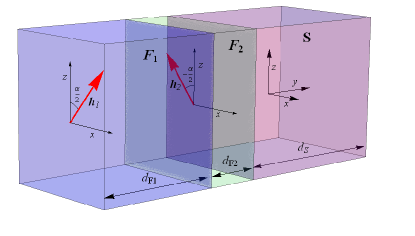
Figure 1: (Color online) Schematic of the F₁F₂S trilayer. The outer ferromagnetic layer $\rm F_{1}$ has a magnetization oriented at an angle $\alpha/2$ in the $x-z$ plane, while the inner ferromagnet, $\rm F_{2}$, has a magnetization orientation at an angle $-\alpha/2$ in the $x-z$ plane. All relevant widths are labeled.

In this paper, we consider several aspects to the proximity effects that arise in $\rm F_{1}F_{2}S$ spin switch nanostructures: We consider arbitrary relative orientation of the magnetic moments in the two F layers and study both the singlet and the induced odd triplet correlations in the clean limit through a fully self-consistent solution of the microscopic Bogoliubov-de Gennes (BdG) equations. We also calculate the critical temperature by solving the linearized BdG equations. As a function of the angle $\alpha$, it is often non-monotonic, possessing a minimum that lies approximately midway between the parallel and antiparallel configurations. Reentrant behavior occurs when this minimum drops to zero. We find that there are induced odd triplet correlations and we study their behavior. These correlations are found to be often long ranged in both the S and F regions. These findings are consistent with the single particle behavior exhibited by the density of states and magnetic moment in these structures.

II Methods

We consider a trilayer ${\rm F_{1}F_{2}S}$ structure infinite in the $x-z$ plane, and with total length $d$ in the $y$ direction, which is normal to the interfaces. The inner ferromagnet layer ($\rm F_{2}$) of width $d_{F2}$ is adjacent to the outer ferromagnet ($\rm F_{1}$) of width $d_{F1}$, and the superconductor has width $d_{S}$ (see Fig. 1). The magnetizations in the ${\rm F_{1}}$ and ${\rm F_{2}}$ layers form angles $\alpha/2$ and $-\alpha/2$, respectively, with the axis of quantization $z$. The superconductor is of the conventional $s$-wave type. We describe the magnetism of the F layers by an effective exchange field ${\bf h}(y)$ that vanishes in the S layer. We assume that interface scattering barriers are negligible, in particular that there is no interfacial spin flip scattering. Our methods are described in Ref. cite:hv2, ; hv2p, and details that are not pertinent to the specific problem we consider here will not be repeated.

To accurately describe the behavior of the quasiparticle ($u_{n\sigma}$) and quasihole ($v_{n\sigma}$) amplitudes with spin $\sigma$, we use the Bogoliubov-de Gennesbdg (BdG) formalism. In our geometry, the BdG equations can be written down after a few stepshv2p in the quasi-one-dimensional form:

$$\begin{pmatrix}{\cal H}_{0}-h_{z}&-h_{x}&0&\Delta(y)\\ -h_{x}&{\cal H}_{0}+h_{z}&\Delta(y)&0\\ 0&\Delta(y)&-({\cal H}_{0}-h_{z})&-h_{x}\\ \Delta(y)&0&-h_{x}&-({\cal H}_{0}+h_{z})\\ \end{pmatrix}\begin{pmatrix}u_{n\uparrow}(y)\\ u_{n\downarrow}(y)\\ v_{n\uparrow}(y)\\ v_{n\downarrow}(y)\end{pmatrix}$$

$$=\epsilon_{n}\begin{pmatrix}u_{n\uparrow}(y)\\ u_{n\downarrow}(y)\\ v_{n\uparrow}(y)\\ v_{n\downarrow}(y)\end{pmatrix},$$ (1)

where ${\cal H}_{0}$ is the usual single particle Hamiltonian, ${\bf h}(y)=(h_{x}(y),0,h_{z}(y))$ is the exchange field in the F layers, $\Delta(y)$ is the pair potential, taken to be real, and the wavefunctions $u_{n\sigma}$ and $v_{n\sigma}$ are the standard coefficients that appear when the usual field operators $\psi_{\sigma}$ are expressed in terms of a Bogoliubov transformation:

$$\psi_{\sigma}({\bf r},t)=\sum_{n}\left(u_{n\sigma}({\bf r})\gamma_{n}e^{-i\epsilon_{n}t}+\eta_{\delta}v_{n\sigma}({\bf r})\gamma_{n}^{\dagger}e^{i\epsilon_{n}t}\right),$$ (2)

where $\eta_{\delta}\equiv 1(-1)$ for spin down (up). We must include all four spin components since the exchange field in the ferromagnets destroys the spin rotation invariance.

To ensure that the system is in an, at least locally, thermodynamically stable state, Eq. (1) must be solved jointly with the self consistency condition for the pair potential:

$$\Delta(y)=\frac{g(y)}{2}{\sum_{n}}^{\prime}\bigl{[}u_{n}^{\uparrow}(y)v^{\downarrow}_{n}(y)+u_{n}^{\downarrow}(y)v^{\uparrow}_{n}(y)\bigr{]}\tanh\Bigl{(}\frac{\epsilon_{n}}{2T}\Bigr{)},\,$$ (3)

where the primed sum is over eigenstates corresponding to positive energies smaller than or equal to the “Debye” characteristic energy cutoff $\omega_{D}$, and $g(y)$ is the superconducting coupling parameter that is a constant $g_{0}$ in the intrinsically superconducting regions and zero elsewhere.

With the above assumptions on interfacial scattering, the triplet correlations are odd in time, in agreement with the Pauli principle and hence vanish at $t=0$. Therefore we will consider the time dependence of the triplet correlation functions, definedcite:hv2 in terms of the usual field operators as,

$$f_{0}({\bf r},t) \equiv\frac{1}{2}[\langle\psi_{\uparrow}({\bf r},t)\psi_{\downarrow}({\bf r},0)\rangle+\langle\psi_{\downarrow}({\bf r},t)\psi_{\uparrow}({\bf r},0)\rangle],$$ (4a)

$$f_{1}({\bf r},t) \equiv\frac{1}{2}[\langle\psi_{\uparrow}({\bf r},t)\psi_{\uparrow}({\bf r},0)\rangle-\langle\psi_{\downarrow}({\bf r},t)\psi_{\downarrow}({\bf r},0)\rangle],$$ (4b)

These expressions can be conveniently written in terms of the quasiparticle amplitudes:cite:hv2 ; hv2p

$$f_{0}(y,t) =\frac{1}{2}\sum_{n}\left[u_{n\uparrow}(y)v_{n\downarrow}(y)-u_{n\downarrow}(y)v_{n\uparrow}(y)\right]\zeta_{n}(t),$$ (5a)

$$f_{1}(y,t) =\frac{1}{2}\sum_{n}\left[u_{n\uparrow}(y)v_{n\uparrow}(y)+u_{n\downarrow}(y)v_{n\downarrow}(y)\right]\zeta_{n}(t),$$ (5b)

where $\zeta_{n}(t)\equiv\cos(\epsilon_{n}t)-i\sin(\epsilon_{n}t)\tanh(\epsilon_{n}/(2T))$, and all positive energy states are in general summed over.

Besides the pair potential and the triplet amplitudes, we can also determine various physically relevant single-particle quantities. One such important quantity is the local magnetization, which can reveal details of the well-known (see among many others, Refs. fryd, ; koshina, ; usold, ; bergeretve, ) reverse proximity effect: the penetration of the magnetization into S. The local magnetic moment ${\bf m}$ will depend on the coordinate $y$ and it will have in general both $x$ and $z$ components, ${\bf m}=(m_{x},0,m_{z})$. We define ${\bf m}=-\mu_{B}\langle\sum_{\sigma}\Psi^{\dagger}{\bm{\sigma}}\Psi\rangle$, where $\Psi^{\dagger}\equiv(\psi_{\uparrow},\psi_{\downarrow})$. In terms of the quasiparticle amplitudes calculated from the self-consistent BdG equations we have,

$$m_{x}(y)= -2\mu_{B}\sum_{n}\biggl{\{}u^{\uparrow}_{n}(y)u^{\downarrow}_{n}(y)f_{n}-v^{\uparrow}_{n}(y)v^{\downarrow}_{n}(y)(1-f_{n})\biggr{\}},$$ (6a)

$$m_{z}(y)= -\mu_{B}\sum_{n}\biggl{\{}(|u^{\uparrow}_{n}(y)|^{2}-|u^{\downarrow}_{n}(y)|^{2})f_{n}$$

$$+(|v^{\uparrow}_{n}(y)|^{2}-|v^{\downarrow}_{n}(y)|^{2})(1-f_{n})\biggr{\}},$$ (6b)

where $f_{n}$ is the Fermi function of $\epsilon_{n}$ and $\mu_{B}$ is the Bohr magneton.

A very useful tool in the study of these systems is tunneling spectroscopy, where information, measured by an STM, can reveal the local DOS (LDOS). Therefore we have computed here also the LDOS $N(y,\epsilon)$ as a function of $y$. We have $N(y,\epsilon)\equiv N_{\uparrow}(y,\epsilon)+N_{\downarrow}(y,\epsilon)$, where,

$$N_{\sigma}(y,\epsilon)=\sum_{n}[u_{n\sigma}^{2}(y)\delta(\epsilon-\epsilon_{n})+v_{n\sigma}^{2}(y)\delta(\epsilon+\epsilon_{n})],\quad\sigma=\uparrow,\downarrow.$$ (7)

The transition temperature can be calculated for our system by finding the temperature at which the pair potential vanishes. It is much more efficient, however, to find $T_{c}$ by linearizingbvh the self-consistency equation near the transition, leading to the form

$$\Delta_{i}=\sum_{q}J_{iq}\Delta_{q},$$ (8)

where the $\Delta_{i}$ are expansion coefficients of the position dependent pair potential in the chosen basis and the $J_{iq}$ are the appropriate matrix elements with respect to the same basis. The somewhat lengthy details of their evaluation are given in Ref. bvh, .

To evaluate the free energy, $F$, of the self-consistent states we use the convenient expression,kos

$$F=-2T\sum_{n}\ln\left[2\cosh\left(\frac{\epsilon_{n}}{2T}\right)\right]+\left\langle\frac{\Delta^{2}(y)}{g(y)}\right\rangle_{s},$$ (9)

where here $\langle\ldots\rangle_{s}$ denotes spatial average. The condensation free energy, $\Delta F$, is defined as $\Delta F\equiv F_{S}-F_{N}$, where $F_{S}$ is the free energy of the superconducting state and $F_{N}$ is that of the non-superconducting system. We compute $F_{N}$ by setting $\Delta\equiv 0$ in Eqs. (1) and (9).

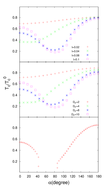
Figure 2: (Color online) Calculated transition temperatures $T_{c}$, normalized to $T_{c}^{0}$. In this figure the two F layers are identical, $D_{F1}=D_{F2}\equiv D_{F}$ and $I_{1}=I_{2}\equiv I$. In the top panel this ratio is shown vs $\alpha$ for different exchange fields at $D_{F}=10$ . In the middle panel the same ratio is plotted again vs $\alpha$ for different values of $D_{F}$ at $I=0.1$. In the bottom panel $T_{c}$ vs $\alpha$ is shown for $D_{F}=6$ and $I=0.15$, a case where reentrance with angle occurs.

III Results

In presenting our results below we measure all lengths in units of the inverse of $k_{F}$ and denote by a capital letter the lengths thus measured. Thus for example $Y\equiv k_{F}y$. The exchange field strength is measured by the dimensionless parameter $I\equiv h/E_{F}$ where $E_{F}$ is the band width in S and $h$ the magnitude of the exchange field ${\bf h}$. In describing the two F layers the subscripts 1 and 2 denote (as in Fig. 1) the outer and inner layers respectively. Whenever the two F layers are identical in some respect the corresponding quantities are given without an index: thus $I_{2}$ would refer to the inner layer while simply $I$ refers to both when this is appropriate. We study a relatively wide range of thicknesses $D_{F1}$ for the outer layer but there would be little purpose in studying thick inner layers beyond the range of the standard singlet proximity effect in the magnets. In all cases we have assumed a superconducting correlation length corresponding to $\Xi_{0}=100$ and measure all temperatures in units of $T_{c}^{0}$, the transition temperature of bulk S material. The quantities $\Xi_{0}$ and $T_{c}^{0}$ suffice to characterize the BCS singlet material we consider. We use $D_{S}=1.5\Xi_{0}$ unless, as otherwise indicated, a larger value is needed to study penetration effects. Except for the transition temperature itself, results shown were obtained in the low temperature limit. For the triplet amplitudes, dimensionless times $\tau$ are defined as $\tau\equiv\omega_{D}t$. Except for this definition, the cutoff frequency plays no significant role in the results.

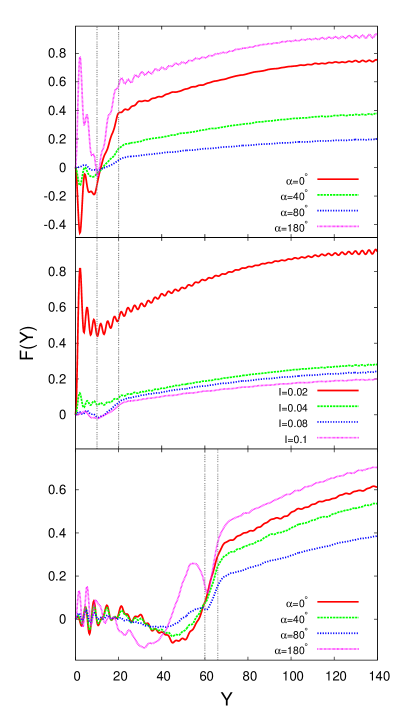
Figure 3: (Color online) Calculated singlet pair amplitude $F(Y)$, normalized to its value in bulk S material, plotted vs $Y\equiv k_{F}y$. In the top panel, results are shown for different $\alpha$ at $I=0.1$ and $D_{F}=10$. The central panel depicts results for the same $D_{F}$, and illustrates the effect of different magnetic strengths, $I$, at fixed $\alpha=80^{\circ}$. The bottom panel shows $F(Y)$ for different $\alpha$ as in the top panel, except for a structure of differing magnet thicknesses: $D_{F1}=60$, and $D_{F2}=6$. The dashed vertical lines represent in each case the location of the ${\rm F_{1}F_{2}}$ and ${\rm F_{2}S}$ interfaces.

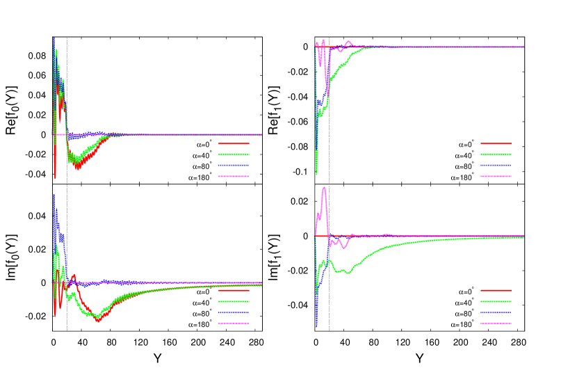
Figure 4: (Color online) The Real and Imaginary parts of the normalized triplet amplitudes $f_{0}$ and $f_{1}$ (see text) plotted vs $Y$ for a sample with $D_{F}=10$, $D_{S}=300$ and $I=0.1$, at dimensionless time $\tau=4.0$. Results are plotted for different values of $\alpha$ as indicated. See text for discussion. Vertical lines indicate, in this and the next three figures, the ${\rm F_{2}S}$ interface. For clarity, the $\rm F_{1}F_{2}$ interface is not included.

III.1 Transition Temperature

The transition temperature $T_{c}$ is calculated directly from the linearization method described in Sec. II. Some of the results are shown in Fig. 2. In this figure we have taken both F layers to be identical and hence both relatively thin. All three panels in the figure display $T_{c}$, normalized to $T_{c}^{0}$, as a function of the angle $\alpha$. The figure dramatically displays, as anticipated in the Introduction, that as opposed to ${\rm F_{1}SF_{2}}$ trilayers, $T_{c}$ does not usually, in our present case, monotonically increase as $\alpha$ increases from 0 to $180^{\circ}$, but on the contrary it has often a minimum at a value of $\alpha$ typically below $90^{\circ}$.

The top panel, which shows results for several intermediate values of $I$ with $D_{F}=10$, illustrates the above statements. $T_{c}$ is found in this case to be monotonic only at the smallest value of $I$ ($I=0.02$) considered. The non-monotonic behavior starts to set in at around $I=0.04$ and then it continues, with the minimum $T_{c}$ remaining at about $\alpha=80^{\circ}$. This is not a universal value: we have found that for other geometric and material parameters the position of the minimum can be lower or higher. In the middle panel we consider a fixed value of $I=0.1$ and several values of $D_{F}$. This panel makes another important point: the four curves plotted in the top panel and the four ones in this panel correspond to identical values of the product $D_{F}I$. The results, while not exactly the same, are extremely similar and confirm that the oscillations in $T_{c}$ are determined by the overall periodicity of the Cooper pair amplitudes in $F$ materials as determined by the difference between up and down Fermi wavevectors, which is approximately proportionalhvlast to $1/I$ in the range of $I$ shown.

In the lowest panel of the figure we show that reentrance with $\alpha$ can occur in these structures. The results there are for $D_{F}=6$ and at $I=0.15$, a value a little larger than that considered in the other panels. While such reentrance is not the rule, we have found that it is not an exceptional situation either: the minimum in $T_{c}$ at intermediate $\alpha$ can simply drop to zero, resulting in reentrance. The origin of this reentrance stems from the presence of triplet correlations due to the inhomogeneous magnetization and the usual $D_{F}$ reentrance in F/S bilayerscite:buzdin ; cite:khusainov ; fominov ; buzdin3 ; hv3 ; hv4 ; bvh , that is, the periodicity of the pair amplitudes mentioned above.

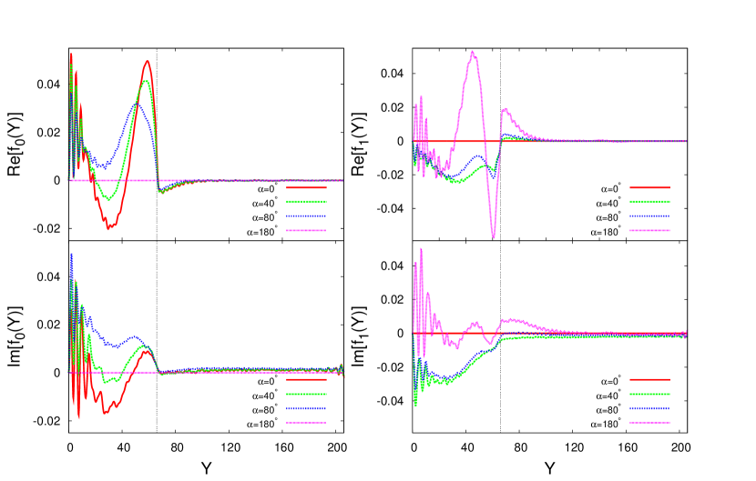
Figure 5: (Color online) The real and imaginary parts of the triplet amplitudes, plotted as in the previous figure except that the sample has $D_{F1}=60,D_{F2}=6$ and $D_{S}=150$. See text for discussion.

III.2 Pair amplitude: singlet

We turn now to the behavior of the standard, singlet pair amplitude $F(y)$, defined as usual via $\Delta(y)\equiv g(y)F(y)$ and Eq. (3), as evaluated from the self consistent calculations described in Sec. II. The behavior of $F(y)$ is rather straightforwardly described and has some features representative of conventional proximity effects found in other ferromagnet-superconductor configurations, such as F/S or ${\rm F_{1}SF_{2}}$ structures. An example is shown in Fig. 3, where that spatial behavior of $F(y)$ is shown for a few cases of exchange fields differing in orientation and magnitude, as well as ferromagnet widths.

The top panel shows results for $F(Y)$ as a function of position, at $I=0.1$ and for several values of $\alpha$, at $D_{F}=10$. We see that in the S layer, the pair amplitude rises steadily over a length scale of order of the correlation length. The variation of the overall amplitude in S with $\alpha$ reflects that of the transition temperature, as was depicted for this case by the (purple) squares in the top panel of Fig. 2. One sees that the non-monotonic trends observed in the critical temperature correlate well with the zero temperature pair amplitude behavior. In the F layers, we observe a more complicated behavior and oscillations with an overall smaller amplitude. These oscillations are characteristic of conventional F/S proximity effects, which in this case appear somewhat chaotic because of reflections and interference at the ${\rm F_{1}F_{2}}$ and end boundaries. This irregular spatial behavior is also due to the chosen value of $I$ and the characteristic spatial periodicity $\approx 2\pi/I$ not matching $D_{F}$. These geometric effects can in some cases, result in the amplitudes of the singlet pair oscillations in ${\rm F_{2}}$ exceeding those in the superconductor near the interface.

In the central panel results for several values of $I$ and the same geometry as the top one are shown where the typical location of the minimum in $T_{c}$ may occur at a relative magnetization angle of $\alpha\approx 80^{\circ}$. We see that for the case $I=0.02$, where $T_{c}$ is high and monotonic with $\alpha$, singlet correlations are significant and they are spread throughout the entire structure. This is consistent with the top panel of Fig. 2, where the critical temperature is highest, and increases only slightly with $\alpha$. For the other values of $I$, there is a strong $T_{c}$ minimum near $\alpha=80^{\circ}$ and consequently, the pair amplitude is much smaller. The weakening of the superconductivity in S inevitably leads to its weakening in the F layers.

The bottom panel demonstrates how the pair amplitude in the structure becomes modified when $\alpha$ is varied, in a way similar to the top panel, except in this case the inner layer is thinner with $D_{F2}=6$ and the outer layer is thicker with $D_{F1}=60$. Comparing the top and bottom panels, we see that clearly geometric effects can be quite influential on the spatial behavior of singlet pairing correlations. In this case the ${\rm F_{2}}$ layer is too thin for $F(Y)$ to exhibit oscillations within it.

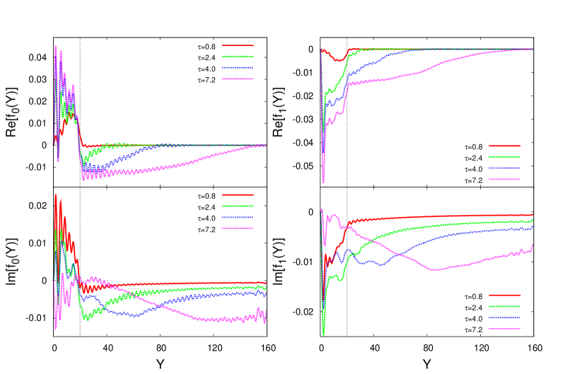
Figure 6: (Color online) The real and imaginary parts of the triplet amplitudes plotted vs $Y$ for the same parameter values and conventions as in Fig. 4, at fixed $\alpha=40^{\circ}$ for several values of $\tau$ as indicated.

III.3 Triplet amplitudes

In this subsection, we discuss the induced triplet pairing correlations in our systems. As mentioned in the Introduction, the triplet pairing correlations may coexist with the usual singlet pairs in F/S heterostructures and their behavior is in many ways quite different: in particular the characteristic proximity length can be quite large. As a function of the angle $\alpha$ the possible existence of the different triplet amplitudes is restrictedcite:hv2 ; hv2p by conservation laws. For instance, at $\alpha=0$ (parallel exchange fields) the $m=\pm 1$ component along our $z$ axis of quantization, $f_{1}(y,t)$, must identically vanish, while $f_{0}$ is allowed. This is because at $\alpha=0$ the $S_{z}$ component of the total Cooper pair spin is conserved, although the total spin quantum number $S$ is not. Neither quantity is conserved for arbitrary $\alpha$. For directions other than $\alpha=0$ restrictions arising from the symmetry properties can be inferredhv2p most easily by projecting onto the $z$ axis the quasiparticle amplitudes along a different axis in the $x-z$ plane via a unitary spin rotation operator, $U$:

$${U}(\varphi)=\cos(\varphi/2)\hat{\bf 1}\otimes\hat{{\bf 1}}-i\sin(\varphi/2)\rho_{z}\otimes\sigma_{y},$$ (10)

where $\varphi$ is measured from the $z$-axis, and $\rho_{z}$ is a Pauli-like operator, acting in particle-hole space. For the anti-parallel case, $\alpha=180^{\circ}$, we have, following from the operation of spin rotation above, the inverse property that only $f_{1}$ components can be induced. In addition, the Pauli principle requires all triplet amplitudes to vanish at $t=0$. We note also that with the usual phase convention taken here, namely that the singlet amplitude is real, the triplet amplitudes may have, and in general they do have, both real and imaginary parts. The results of triplet amplitudes shown here are calculated at zero temperature and are normalized to the singlet pair amplitude of a bulk S material.

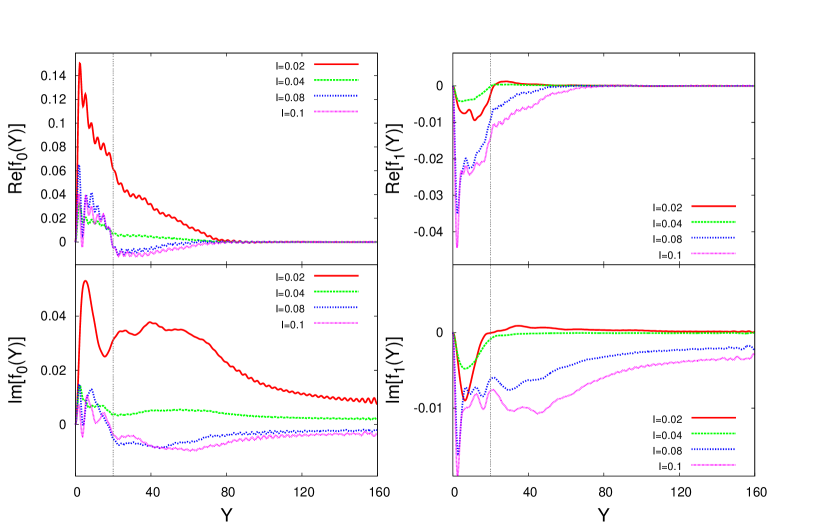
Figure 7: (Color online) The triplet amplitudes $f_{0}$ and $f_{1}$ plotted as a function of position at fixed $\alpha=40^{\circ}$ and $\tau=4$ for several values of $I$. We have here $D_{F}=10$, and $D_{S}=150$.

First, we present in Fig. 4 the case of a thick S layer ($D_{S}=300$) with two thin F layers ($D_{F}=10$). The two F layers have exchange fields of identical magnitude, corresponding to $I=0.1$, and the angle $\alpha$ is varied. The dimensionless time chosen is $\tau=4$, the behavior is characteristic of all times in the relevant range. Of course the results at $\tau=0$ are found to vanish identically. As observed in this figure, the results for $f_{1}$ vanish at $\alpha=0$ and those for $f_{0}$ at $\alpha=\pi$ in agreement with the conservation law restrictions. We see that the triplet amplitudes can be quite long ranged in S: this is evident, with our phase convention, for the imaginary parts of $f_{0}$ and $f_{1}$ at $\alpha=40^{\circ}$. Thus the triplet correlations for this particular magnetization orientation can penetrate all the way to the other end of the S side, even though the S layer is three coherence lengths thick. In addition, one can see that antiparallel magnetizations in the F layers lead to both the real parts and the imaginary parts of $f_{1}$ being short ranged. Non-collinear relative orientations of the exchange fields in the inner and outer F layers may induce both long range $f_{0}$ and $f_{1}$ components simultaneously. However, the triplet pairing correlations for $\alpha=80^{\circ}$ are not as long ranged as those for $\alpha=40^{\circ}$. This can be indirectly attributed to much weaker singlet amplitudes inside S in the former case: the overall superconductivity scale is still set by the singlet, intrinsic correlations. Considering now the real parts of $f_{0}$ and $f_{1}$, and other than parallel and antiparallel magnetizations, the penetration of $f_{0}$ correlations within the ferromagnet regions is weakly dependent on the angle $\alpha$, while $f_{1}$ is more sensitive to $\alpha$. Within the superconductor we see similar trends as for the imaginary parts except that the real components of $f_{1}$ and $f_{0}$ extend over a shorter distance within S at the same $\tau$ value.

Motivated by the long range triplet amplitudes found above for an ${\rm F_{1}F_{2}S}$ structure with relatively thin F layers and a thick S layer, we discuss next, in Fig. 5, the case of a thicker outer ferromagnet layer with $D_{F1}=60$, with $D_{S}=150$. The values of $\tau$ and $I$ are the same as in Fig. 4. Fig. 5 shows that the triplet amplitudes are more prominent in the F than in the S regions. There is also an underlying periodicity that is superimposed with apparent interference effects, with a shorter period than that found in the singlet pair amplitudes (see bottom panel, Fig. 3). Also, the imaginary component of $f_{0}$ penetrates the superconductor less than the imaginary $f_{1}$ component. For the real $f_{1}$ component, the exchange field of the inner layer produces a valley near the interface in the F regions. This feature is most prominent when the exchange fields are anti-parallel, in which case the equal-spin triplet correlations are maximized. Aside from this, the triplet amplitudes in S are smaller than in the case above with thicker S and thinner $F_{1}$, although their range is not dissimilar. This is mainly because the triplet penetration into S is appreciably affected by finite size effects: When one of the F layers is relatively thick, it is only after a longer time delay $\tau$ that the triplet correlations evolve. From Fig. 5, one can also see that the triplet $f_{0}$ correlations in S are nearly real (i.e. in phase with the singlet) and essentially independent of the angle $\alpha$.

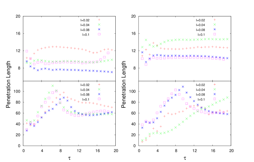
Figure 8: (Color online) Study of the triplet penetration lengths, see Eq. (11), vs $\tau$. In this figure, $D_{F}=10$, $D_{S}=150$, and $\alpha=40^{\circ}$. Left panels: lengths as extracted from $f_{0}(Y)$ for several values of $I$ in the $F$ regions (top panel) and in the $S$ region (bottom panel). The right panels contain the same information, arranged in the same way, but with the penetration length extracted from $f_{1}(Y)$. The lengths eventually saturate.

The triplet penetration is a function of the characteristic time $\tau$ scales. We therefore study the dependence of the triplet amplitudes on $\tau$ in Fig. 6, which shows results corresponding to $D_{F}=10$, $D_{S}=150$, $\alpha=40^{\circ}$, $I=0.1$, and at four different values of $\tau$. Again, the triplet amplitudes, particularly their imaginary parts, are long range. The plots clearly show that at short times, $\tau=0.8$, the triplet correlations generated at the interface reside mainly in the F region. At larger values of $\tau$, the triplet amplitudes penetrate more deeply into the S side, and eventually saturate. For the range of times shown, the magnitude of the real parts of $f_{0}$ and $f_{1}$, decays in the S region near the interface due to the phase decoherence associated with conventional proximity effects. For the largest value of $\tau=7.2$ in the figure, the imaginary parts of $f_{0}$ and $f_{1}$ do not display monotonic decrease on the S side of the interface but saturate. This is because for these values of $\tau$ the triplet amplitudes already pervade the entire S. This indicates that both triplet components infiltrate the superconductor more efficiently and at smaller values of $\tau$ when they are nearly out of phase with the singlet amplitude.

We also investigated the dependence of the triplet amplitudes on the magnitude of exchange field at a set time, $\tau=4$. Fig. 7 illustrates the real and imaginary parts of the complex $f_{0}$ (left panels) and $f_{1}$ (right panels). The geometric parameters are $D_{F}=10$, and $D_{S}=150$, and we consider four different $I$ values at fixed relative orientation, $\alpha=40^{\circ}$. In our discussion below, we divide these four different values into two groups, the first including the two smaller values, $I=0.02$ and $I=0.04$, and the second the two somewhat larger ones, $I=0.08$ and $I=0.1$. In each group, the triplet amplitudes are similar in shape but different in magnitude. For the first group, there are no nodes at the ${\rm F_{2}S}$ interface for the $f_{0}$ components, while the $f_{1}$ components cross zero near it. For the second group, the opposite occurs: the $f_{0}$ components cross zero while the $f_{1}$ components do not. Also, the ratio of ${\rm Re}[f_{0}]$ at $I=0.04$ to ${\rm Re}[f_{0}]$ at $I=0.02$ is comparable to the ratio for the corresponding singlet amplitudes. This can be inferred, see Fig. 2, from the transition temperatures for $I=0.02$, which are higher than $I=0.04$. Furthermore, the transition temperatures for the first group are monotonically increasing with $\alpha$, while for the second group, they are non-monotonic functions with a minimum around $\alpha=80^{\circ}$. Therefore, the $f_{0}$ triplet amplitudes are indeed correlated with singlet amplitudes and the transition temperatures also reflect their behaviors indirectly.

There is an interesting relationship involving the interplay between singlet and equal-spin triplet amplitudes: When $T_{c}$ is a non-monotonic function of $\alpha$, the singlet amplitudes (which are directly correlated with $T_{c}$) at the angle where $T_{c}(\alpha)$ has a minimum are partly transformed into equal spin triplet amplitudes. By looking at the central panel of Fig. 2, one sees that the transition temperatures for $I=0.08$ and $I=0.1$ nearly overlap, while the $I=0.02$ case has a much higher transition temperature around $\alpha=80^{\circ}$. The singlet pair amplitudes (at zero temperature) follow the same trend as well: at $I=0.02$, $F(Y)$ is much larger than the other pair amplitudes at different $I$ (see the middle panel of Fig. 3). The $f_{1}$ component for these cases however, shows the opposite trend (see, e.g., the right panels of Fig. 7): for $I=0.08$ and $I=0.1$, the equal spin correlations extend throughout the S region, but then abruptly plummet for $I=0.02$. This inverse relationship between ordinary singlet correlations and $f_{1}$ is suggestive of singlet-triplet conversion for these particular magnetizations in each ferromagnet layer.

Having seen that the triplet amplitudes generated by the inhomogeneous magnetization can extend throughout the sample in a way that depends on $\tau$, we proceed now to characterize their extension by determining a characteristic triplet proximity length. We calculate the characteristic lengths, $l_{i}$, from our data for the triplet amplitudes, by using the same definition as in previoushv2p work:

$$l_{i}=\dfrac{\int dy|f_{i}(y,\tau)|}{\max|f_{i}(y,\tau)|},\quad i=0,1,$$ (11)

where the integration is either over the superconducting or the magnetic region. The normalization means that these lengths measure the range, not the magnitude, of the induced correlations. In Fig. 8 we show results for the four lengths thus obtained, for a sample with $D_{F}=10$, $D_{S}=150$ and $\alpha=40^{\circ}$, at several values of $I$. The left panels show these lengths for the $f_{0}$ component, and the right panels show the results for the corresponding $f_{1}$ component. The triplet penetration lengths in the $F$ region are completely saturated, even at smaller values of $\tau$, for both $f_{0}$ and $f_{1}$. This saturation follows only in part from the relatively thin F layers used for the calculations in this figure: the same saturation occurs for the geometry of Fig. 5 where $D_{F1}+D_{F2}=66$, although of course at much larger values of $l_{i}$. The triplet correlations easily pervade the magnetic part of the sample. On the other hand, the corresponding penetration lengths for both triplet correlations, $f_{0}$ and $f_{1}$, in the S region are substantially greater and, because $D_{S}$ is much larger, do not saturate but possess a peak around $\tau=8$ in all cases except for $f_{1}$ at lager $I$ where it is beyond the figure range. The behavior for the sample with larger F thicknesses is, on the S side, qualitatively similar.

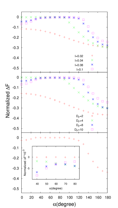
Figure 9: (Color online) Normalized condensation free energies $\Delta F$ vs $\alpha$, at $T=0$. The three panels are for the same geometry and parameter values as in Fig. 2, and the symbols have the same meaning. Thus the top panel corresponds to $D_{F}=10$ and several values of $I$, while the middle panel is for $I=0.1$ and several values of $D_{F}$. The bottom panel corresponds to the reentrant case shown in the corresponding panel of Fig. 2. The inset shows the difference between truly reentrant cases and those for which the condensation energy is small (see text) in the range of $\alpha=40^{\circ}$ to $\alpha=80^{\circ}$.

III.4 Thermodynamics

Given the self-consistent solutions, we are able to compute also the thermodynamic functions. In particular, we obtained the condensation free energies $\Delta F=F_{S}-F_{N}$ by using Eq. 9. In Fig. 9, we plot calculated results for $\Delta F$ at zero $T$, equivalent to the condensation energy. We normalize $\Delta F$ to $N(0)\Delta_{0}^{2}$, where $N(0)$ denotes the density of states at the Fermi level and $\Delta_{0}$ denotes the bulk value of the singlet pair potential in S: thus we would have $\Delta F=-0.5$ for pure bulk S. The three panels in this figure correspond to those in Fig. 2. The geometry is the same and the symbol meanings in each panel correspond to the same cases, for ease of comparison. In the top panel, we see that the $\Delta F$ curves for $I=0.02$ and $I=0.04$ are monotonically decreasing with $\alpha$. This corresponds to the monotonically increasing $T_{c}$. One can conclude that the system becomes more superconducting when $\alpha$ is changing from parallel to anti-parallel: the superconducting state is getting increasingly more favorable than the normal one as one increases the tilt from $\alpha=0$ to $\alpha=\pi$. The other two curves in this panel, which correspond to $I=0.08$ and $I=0.1$, show a maximum near $\alpha=80^{\circ}$. Again, this is consistent with the transition temperatures shown in Fig. 2. Comparing also with the middle panel of Fig. 3, we see that the singlet amplitude for $I=0.02$ is much larger than that for the other values of $I$. This is consistent with Fig. 9: $\Delta F$ is more negative at $I=0.02$ and the superconducting state is also more stable. The middle panel of Fig. 9 shows $\Delta F$ for different ferromagnet thicknesses. The curves are very similar to those in the top panel, just as the top two panels in Fig. 2 were found to be similar to each other. Therefore, both Fig. 2 and Fig. 9, show that the superconducting states are thermodynamically more stable at $\alpha=180^{\circ}$ than in the intermediate regions ($\alpha=40^{\circ}$ to $\alpha=80^{\circ}$). From the top two panels in Fig. 9, we also see that $\Delta F$ at $\alpha=180^{\circ}$ can be near $-0.3$ in this geometry: this is a very large value, quite comparable to that in pure bulk S. However, in the region of the $T_{c}$ minima near $\alpha=80^{\circ}$, the absolute value of the condensation energy can be over an order of magnitude smaller, although it remains (see below) negative. The bottom panel of Fig. 9 shows $\Delta F$ for the reentrant case previously presented in Fig. 2, for which $D_{F}=6$ and $I=0.15$. The main plot shows the condensation energy results, which vanish at intermediate angles. Because $\Delta F$ in the intermediate non-reentrant regions shown in the upper two panels can be very small, in the vertical scale shown, we have added to the lowest panel an inset where the two situations are contrasted. In the inset, the (red) plus signs represent $\Delta F$ for the truly reentrant case and the other three symbols have the same meaning as in the middle panel, where no reentrance occurs. The inset clearly shows the difference: $\Delta F$ vanishes in the intermediate region only for the reentrant $T_{c}$ case and remains slightly negative otherwise. The pair amplitudes for the reentrant region are found self-consistently to be identically zero. Thus one can safely say that in the intermediate region the system must stay in the normal state and no self-consistent superconducting solution exists. Evidence for reentrance with $\alpha$ in $\rm F_{1}F_{2}S$ is therefore found from both the microscopic pair amplitude and from $T_{c}$: it is also confirmed thermodynamically. That superconductivity in ${\rm F_{1}F_{2}S}$ trilayers can be reentrant with the angle between $\rm F_{1}$ and $\rm F_{2}$ layers, makes these systems ideal candidates for spin-valves.

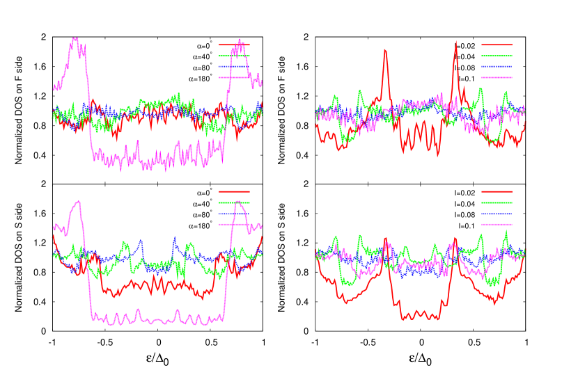
Figure 10: (Color online) LDOS integrated over the $F$ layers (top panels) and the $S$ layer (bottom panels). In all cases $D_{F}=10$, $D_{S}=150$, and $T=0.05T_{c}^{0}$. The left panels show results for $I=0.1$ and the indicated values of $\alpha$, while in the right panels we have $\alpha=40^{\circ}$ and several values of $I$.

III.5 DOS

Next, we present some results for the local DOS (LDOS) in $\rm F_{1}F_{2}S$ systems. All plots are normalized to the corresponding value in a bulk sample of S material in its normal state. The top panels in Fig. 10 show the normalized LDOS integrated over the entire magnetic portion of the sample, while in the bottom panels the LDOS is integrated over the S region. In all four cases we use $D_{F}=10$, $D_{S}=150$. In the left panels we have fixed $I=0.1$ and present results for several angles, while in the right panels we take a fixed $\alpha=40^{\circ}$ and show results for several values of $I$ as indicated. In the top left panel (F side) we see no energy gap for any value of $\alpha$, however a flat valley between two peaks for the case $\alpha=180^{\circ}$ resembles a characteristic feature of the DOS in bulk superconductors. However, the plots at the other three angles, where the transition temperature and condensation energies are much lower, are very near the value of the DOS in its normal state throughout all energies. This is also consistent with the top panel of Fig. 3, where the Cooper pair amplitudes in this case are larger inside F most significantly at $\alpha=180^{\circ}$. The singlet amplitudes at $\alpha=0$ are also larger than in the other non-collinear configurations, but the superconducting feature in the LDOS is not as prominent. This could be due to the contributions from the triplet pairing correlations: We know from the spin symmetry arguments discussed above that there is no $f_{1}$ component of the induced triplet amplitude at $\alpha=0^{\circ}$ and therefore it can not enhance the superconducting feature in the DOS. On the contrary, both singlet and triplet amplitudes can contribute when $\alpha=180^{\circ}$. Thus the LDOS results in the F side reflect the signature of induced triplet amplitudes in $\rm F_{1}F_{2}S$ systems.

The left bottom panel displays the integrated LDOS over the entire S layers for the same parameters as the top one. Again, the plot for $\alpha=180^{\circ}$, corresponding to the highest $T_{c}$ and most negative condensation energy, possesses a behavior similar to that in pure bulk S material, although the wide dip in the DOS does not quite reach down to zero. On the other hand, the LDOS at $\alpha=80^{\circ}$, the case with the most fragile superconductivity, has a shallow and narrow valley. The DOS plots on the left side are very similar to the normal state result both at $\alpha=40^{\circ}$ and at $\alpha=80^{\circ}$. In summary, the depth and the width of the dip are mostly correlated with the singlet pair amplitudes. The left panels also support our previous analysis: the slight difference between the normal states and superconducting states in the intermediate angle region is reflected in the DOS. The right panels reveal how the magnetic strength parameter, $I$, affects the integrated DOS. As we can see from the middle panel in Fig. 3, the singlet Cooper pair amplitudes for this case drop significantly when $I\geq 0.04$. The right panels in Fig. 10 confirm this information, that is the integrated DOSs in both the F and S sides have a very noticeable dip in the F side, and a near gap on the S region for $I=0.02$ , while for the other vaues of $I$ the eveidence for superconductivity in the DOS is much less prominent.

III.6 Local magnetization

Finally, it is also important to study the reverse proximity effects: not only can the superconductivity penetrate into the ferromagnets, but conversely the electrons in S near the interface can be spin polarized by the presence of the F layers. This introduction of magnetic order in S is accompanied by a corresponding decrease of the local local magnetization in ${\rm F_{2}}$ near the S interface. In Fig. 11, we show the components of the local magnetization, as defined in Eq. 6. The parameters used are $D_{F}=10$, $D_{S}=150$ and $I=0.1$ and results are shown for different values of $\alpha$. The local magnetization results shown are normalized by $-\mu_{B}(N_{\uparrow}+N_{\downarrow})$, where $N_{\uparrow}=k_{F}^{3}(1+I)^{3/2}/6\pi^{2}$ and $N_{\downarrow}=k_{F}^{3}(1-I)^{3/2}/6\pi^{2}$. From the figure one sees at once that both the sign and average magnitude of the $m_{x}$ and $m_{z}$ components inside the F material are in accordance with the values of the angle $\alpha$ and of the exchange field ($I=0.1$). As to the reverse proximity effect, we indeed see a nonzero value of the local magnetization in S near the the interface. The penetration depth corresponding to this reverse effect is independent of $\alpha$. Unlike the singlet and triplet amplitudes, which may spread throughout the entire structure, the local magnetizations can only penetrate a short distance. This is consistent with results from past workcite:hv2 .

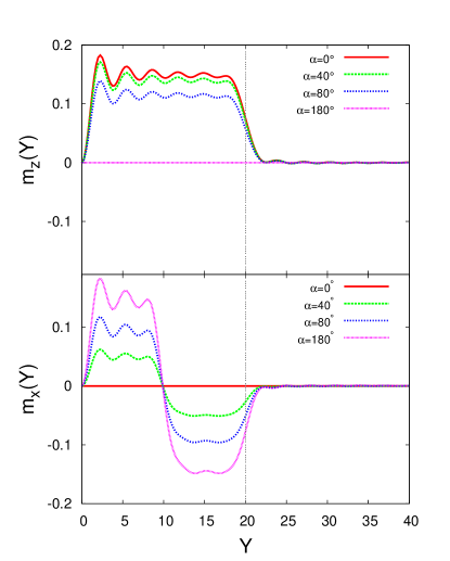
Figure 11: (Color online) The $z$ component (top panel) and the x component (bottom panel) of the local magnetization, plotted as a function of $Y$ for several $\alpha$ values. We use $D_{F}=10$, $D_{S}=150$, and $I=0.1$ in this figure.

IV Summary and Conclusions

In summary, we have investigated the proximity effects in ${\rm F_{1}F_{2}S}$ trilayers by self-consistently solving the BdG equations. One of the most prominent features of these systems, which make them different from $\rm F_{1}SF_{2}$ structures is the non-monotonicity of $T_{c}(\alpha)$, as the angle, $\alpha$, between adjacent magnetizations is varied. For $\rm F_{1}SF_{2}$ systems the critical temperature is always lowest for parallel ($\alpha=0^{\circ}$) orientations, due chiefly to the decreased average exchange field as $\alpha$ increases and the two F’s increasingly counteract one another. In contrast, we find that $\rm F_{1}F_{2}S$ configurations can exhibit for particular combinations of exchange field strengths and layer thicknesses, critical temperatures that are lowest for relative magnetization orientations at an intermediate angle between the parallel and antiparallel configurations. In some cases the drop in $T_{c}$ from the parallel state, as $\alpha$ is varied, is large enough that superconductivity is completely inhibited over a range of $\alpha$, and then reemerges again as $\alpha$ increases: the system exhibits reentrant superconductivity with $\alpha$. We also calculated the singlet pair amplitude and condensation energies at zero temperature, revealing behavior that is entirely consistent with these findings.

We have studied the odd triplet amplitudes that we find are generated, and found that both the opposite spin pairing (with $m=0$) amplitude, $f_{0}$, and the equal-spin pairing amplitude (with $m=\pm 1$), $f_{1}$, can be induced by the inhomogeneous exchange fields in the F layers. Also of importance, we have shown that the triplet pairing correlations can be very long ranged and extend throughout both the F and S regions, particularly for relatively thick S and F layers. We have characterized this penetration by calculating and analyzing properly defined characteristic lengths. We have also shown that the inner $\rm F_{2}$ layer, when its exchange field is not aligned with that of the outer $\rm F_{1}$ layer, plays an important role in generating the triplet amplitudes. When both magnets are thin, there is an indirect relationship between the singlet pairing amplitudes that govern $T_{c}$ and the $f_{1}$ amplitudes that govern the behavior of equal-spin pairing. We have also presented calculations of the energy resolved DOS, spatially averaged over the S or F regions, demonstrating clear signatures in the energy spectra, which can be identified depending on the relative magnetization vectors in the $\rm F_{1}$ and $\rm F_{2}$ regions. We have determined that the extent of magnetic leakage into the S region as extracted from a calculation of the components of the local magnetization, is rather short ranged. Throughout this paper, we have emphasized the potential of these structures as ideal candidates for spin valves.

- (1) I. Zutić, J. Fabian, and S. Das Sarma, Rev. Mod. Phys. 76, 323 (2004).
- (2) A. I. Buzdin, Rev. Mod. Phys. 77, 935 (2005).
- (3) K. Halterman and O. T. Valls, Phys. Rev. B 66, 224516 (2002).
- (4) E. A. Demler, G. B. Arnold, and M. R. Beasley, Phys. Rev. B 55, 15174 (1997).
- (5) A. F. Andreev, Sov. Phys. JETP 19, 1228 (1964).
- (6) Z. Radović, et al., Phys. Rev. B 44, 759 (1991).
- (7) J. S. Jiang, D. Davidović, D. H. Reich, and C. L. Chien, Phys. Rev. Lett. 74, 314 (1995).
- (8) M. G. Khusainov and Y. N. Proshin, Phys. Rev. B 56, R14283 (1997).
- (9) I. A. Garifullin et al., Phys. Rev. B 66, 020505(R) (2002).
- (10) V. Zdravkov et al., Phys. Rev. Lett. 97, 057004 (2006).
- (11) Y. V. Fominov, N. M. Chtchelkatchev, and A. A. Golubov, Phys. Rev. B 66, 014507 (2002)
- (12) I. Baladié and A. Buzdin, Phys. Rev. B 67, 014523 (2003).
- (13) K. Halterman and O. T. Valls, Phys. Rev. B 70, 104516 (2004).
- (14) K. Halterman and O. T. Valls, Phys. Rev. B 72, 060514(R) (2005).
- (15) F.S. Bergeret, A.F. Volkov, and K.B. Efetov, Phys. Rev. Lett. 86, 3140 (2001).
- (16) F.S. Bergeret, A.F. Volkov, and K.B. Efetov, Phys. Rev. B 68, 064513 (2003); Rev. Mod. Phys. 77, 1321 (2005).
- (17) T. Löfwander et al., Phys. Rev. Lett. 95, 187003 (2005).
- (18) K. Halterman, P. H. Barsic, and O. T. Valls, Phys. Rev. Lett. 99, 127002 (2007).
- (19) K. Halterman, O. T. Valls, P. H. Barsic, Phys. Rev. B 77, 174511, (2008).
- (20) V. L. Berezinskii, JETP Lett. 20, 287, (1974).
- (21) M. Giroud, et al., Phys. Rev. B 58, R11872 (1998).
- (22) T.S. Khaire et al., Phys. Rev. Lett. 104 137002 (2010).
- (23) J.Y. Gu, J. Kusnadi and C.-Y. You, Phys. Rev. B81, 214435 (2010).
- (24) D. Springmann et al. Phys. Rev. B82, 060505 (2010).
- (25) J. W. A. Robinson, J. D. S. Witt, and M. G. Blamire, Science 329, 59 (2010).
- (26) C.-T. Wu, O. T. Valls, and K. Halterman, Phys. Rev. Lett. 108, 107005 (2012).
- (27) M. Eschrig and T. Löfwander, Nature Physics 4, 138 (2008).
- (28) M. Eschrig et al, Phys. Rev. Lett. 90, 137003 (2003). J. Low temp. Phys, 147, 457 (2007).
- (29) M. Grein et al. Phys. Rev. Lett. 102, 227005 (2009).
- (30) Ya. V. Fominov, et al., JETP Letters 91, 308 (2010).
- (31) S. Oh, D. Youm, and M. R. Beasley, Appl. Phys. Lett. 71, 2376 (1997).
- (32) T. Y. Karminskaya, A. A. Golubov, and M. Y. Kupriyanov, Phys. Rev. B 84, 064531 (2011).
- (33) Q. Cheng, and B. Jin, Physica C 473, 29 (2012).
- (34) M. Knežević, L. Trifunovic, and Z. Radović, Phys. Rev. B 85, 094517 (2012).
- (35) J. Zhu, I. N. Krivorotov, K. Halterman, and O. T. Valls, Phys. Rev. Lett. 105, 207002 (2010) and references therein.
- (36) L. R. Tagirov., Phys. Rev. Lett. 83, 2058 (1999).
- (37) A. I. Buzdin, A. V. Vedyayev, and N. V. Ryzhanova, Europhys. Lett. 48, 686 (1999).
- (38) J. Y. Gu., et al., Phys. Rev. Lett. 89, 267001 (2002).
- (39) A. Potenza and C. H. Marrows, Phys. Rev. B 71, 180503(R) (2005).
- (40) I. C. Moraru, W. P. Pratt, Jr., and N. O. Birge, Phys. Rev. Lett. 96, 037004 (2006).
- (41) P. V. Leksin, et al., Appl. Phys. Lett. 97, 102505 (2010).
- (42) P. V. Leksin, et al., Phys. Rev. Lett. 106, 067005 (2011).
- (43) K. Westerholt, et al., Phys. Rev. Lett. 95, 097003 (2005).
- (44) G. Nowak, et al., Phys. Rev. B 78, 134520 (2008).
- (45) P. G. de Gennes, Superconductivity of Metals and Alloys (Addison-Wesley, Reading, MA, 1989).
- (46) A. Frydman and R.C. Dynes, Phys. Rev. B 59, 8432, (1999).
- (47) V.N. Krivoruchko and E. A. Koshina, Phys. Rev. B 66, 014521 (2002).
- (48) K. Halterman and O.T. Valls, Phys. Rev. B65, 014509 (2001); Phys. Rev. B69, 014517 (2004).
- (49) F.S. Bergeret, A.F. Volkov, and K.B. Efetov, Phys. Rev. B 69, 174504 (2004).
- (50) P. H. Barsic, O. T. Valls, and K. Halterman, Phys. Rev. B 75, 104502 (2007).
- (51) I. Kosztin, Š. Kos, M. Stone, A. J. Leggett, Phys. Rev. B 58, 9365 (1998).
- (52) K. Halterman and O. T. Valls, Phys. Rev. B 65, 014509, (2002).