New physics for muon anomalous magnetic moment and its electroweak precision analysis

(a)Shunichi Kanemitsu and (a,b)Kazuhiro Tobe


(a)Department of Physics, Nagoya University, Nagoya 464-8602, Japan

(b)Kobayashi-Maskawa Institute for the Origin of Particles and the Universe,
Nagoya University, Nagoya 464-8602, Japan


About 3σ𝜎\sigma deviation from the standard model prediction of muon anomalous magnetic moment (muon g-2) has been reported. We consider new physics beyond the standard model which has new Yukawa interactions with muon. We compute new contributions to muon g-2 and corrections to electroweak observables, and show the consistent region of parameter space. We find that in a simple model where the chirality flip of muon occurs only in the external muon line in one-loop muon g-2 diagrams, it is necessary to introduce the relatively large new Yukawa coupling and the electroweak scale new particles. On the other hand, in a model where the chirality flip can occur in the internal fermion line of one loop muon g-2 diagrams, we can obtain favorable g-2 contributions without large Yukawa coupling, and they are consistent with the precision electroweak observables. Finally, we discuss effects of new particles for muon g-2 on the Higgs boson decay hγγ𝛾𝛾h\rightarrow\gamma\gamma and direct productions of these particles at the LHC experiment.

1 Introduction

The standard model of elementary particles (SM) has been amazingly successful, and currently the Large Hadron Collider (LHC) experiment is searching for Higgs boson, which is the only particle that has not been observed yet in the framework of the SM. So far, some interesting hints of the Higgs boson with a mass of about 125 GeV have been reported at the LHC [1] and its discovery may not be in a far future. The Higgs boson with a mass of about 100 GeV is totally consistent with the electroweak (EW) precision measurements. Therefore, the SM well-describes the nature up to the EW scale.

We, however, think that the SM is not the final theory of elementary particles. The hierarchy problem has been a strong driving force to think of the physics beyond the SM, and many ideas, such as supersymmetry, extra-dimension, and technicolor, have been proposed to solve the problem. The LHC experiment is an ideal place to probe the models for the hierarchy problem, and the searches are currently going on. The first round of the LHC searches, however, does not show any serious deviations from the SM prediction. It seems that this negative search result starts creating a tension between new physics models and the requirements for the hierarchy problem. Therefore it will be good time to consider other approaches to think about new physics beyond the SM.

There is a different approach to consider the physics beyond the SM, based on a consideration for unexplained experimental results. The muon anomalous magnetic moment (muon g-2) is one of the most precisely measured observables [2]. The theoretical prediction from the SM by several groups has suggested that there is a discrepancy between the experimental result and the SM prediction [3]:

δaμaμexpaμSM=(26.1±8.0)×1010,𝛿subscript𝑎𝜇superscriptsubscript𝑎𝜇expsuperscriptsubscript𝑎𝜇SMplus-or-minus26.18.0superscript1010\displaystyle\delta a_{\mu}\equiv a_{\mu}^{\rm exp}-a_{\mu}^{\rm SM}=(26.1\pm 8.0)\times 10^{-10}, (1.1)

where δaμ𝛿subscript𝑎𝜇\delta a_{\mu} is a discrepancy between the experimental result (aμexp)superscriptsubscript𝑎𝜇exp(a_{\mu}^{\rm exp}) and the SM prediction (aμSM)superscriptsubscript𝑎𝜇SM(a_{\mu}^{\rm SM}). There are many discussions [3, 4] on uncertainties of the SM prediction to understand whether this anomaly is real or not. If the discrepancy can not be explained by the SM, this would be an evidence of the physics beyond the SM. At present, there seems no satisfactory explanation for this anomaly within the SM. Therefore, it is worth while considering the physics beyond the SM seriously in order to explain the anomaly.

It is interesting to note that the anomaly of muon g-2 is the same size as 1-loop contributions induced by the EW gauge bosons in the SM. This suggests that in order to explain the anomaly, new particles with masses of EW scale are required if the interactions are of order of EW gauge couplings.

Although the anomaly of muon g-2 has been discussed in the context of new physics models (for example, see Ref. [5] in MSSM, Ref. [6] in extra dimension model, and Ref. [7] in Little Higgs model) motivated mainly by the hierarchy problem, we take a “bottom-up” style approach #1#1#1 See also Ref. [8] for the recent related studies.. Starting from introducing new interactions with muon to generate new contribution to muon g-2, we try to capture important features of new physics models, although we can only discuss a part of complete models. In this paper, we consider models where muon has new Yukawa type interactions with new particles to generate new contributions to muon g-2. We find that in a model where the chirarity flip of muon occurs only in external line of muon g-2 diagrams, it is necessary to introduce the relatively large Yukawa coupling and the EW scale new particles. On the other hand, in a model where the chirality flip can happen in the internal lines of muon g-2 diagrams, we can obtain favorable g-2 contributions without large Yukawa couplings, and they are also consistent with the precision EW observables. We also expect these particles may be observed directly and/or indirectly at the LHC experiment.

This paper is organized as follows. In the next section, we consider new physics models where muon has new Yukawa couplings to explain the anomaly of muon g-2. One model is that only right-handed muon has new Yukawa coupling. Another one is that both right- and left- handed muons have new Yukawa interactions to enhance the contributions to the muon g-2. We show the consistent region of parameter space. In Sec. 3, we discuss effects of the new physics on EW observables and whether the parameter space which is consistent with the muon g-2 is also consistent with the precision measurements. In Sec. 4, we discuss phenomenology of these new physics models at the LHC. Especially we show the possible effect on the Higgs boson decay of hγγ𝛾𝛾h\rightarrow\gamma\gamma, and the direct production cross sections of new particles at the LHC. Sec. 5 is devoted to summary.

2 New physics models for anomaly of muon g-2

In order to explain the deviation from the SM prediction of muon g-2 by new physics, muon has to have new interactions with some charged particles. Since the effective operator for muon g-2 couples to photon, the loop effects via the new interactions of muon with charged particles could induce the extra contribution to the muon g-2.

In this paper, as such new interactions, we consider new Yukawa-type couplings with right-handed or/and left-handed muon. We consider two cases: (1) Model where only right-handed muon has new Yukawa interaction and (2) Model where both right-handed and left-handed muons have new Yukawa interactions.

2.1 Model where right-handed muon has new Yukawa interaction with SU(2) singlet scalar (ϕitalic-ϕ\phi) and singlet Dirac fermion (χ𝜒\chi)

We consider the following Yukawa interaction where the right-handed muon couples to new SU(2)Lsubscript2𝐿(2)_{L} singlet fermion χ𝜒\chi and singlet scalar ϕitalic-ϕ\phi:

=yNμ¯RχLϕmχχ¯RχL+h.c.mϕ2ϕϕ+.formulae-sequencesubscript𝑦𝑁subscript¯𝜇𝑅subscript𝜒𝐿italic-ϕsubscript𝑚𝜒subscript¯𝜒𝑅subscript𝜒𝐿hcsuperscriptsubscript𝑚italic-ϕ2superscriptitalic-ϕitalic-ϕ\displaystyle{\cal L}=-y_{N}\bar{\mu}_{R}\chi_{L}\phi-m_{\chi}\bar{\chi}_{R}\chi_{L}+{\rm h.c.}-m_{\phi}^{2}\phi^{\dagger}\phi+{\cdots}. (2.2)

Here μRsubscript𝜇𝑅\mu_{R} is the right-handed muon. QED charges of new fermion χ𝜒\chi and scalar ϕitalic-ϕ\phi are Qχsubscript𝑄𝜒Q_{\chi} and Qϕ=1Qχsubscript𝑄italic-ϕ1subscript𝑄𝜒Q_{\phi}=-1-Q_{\chi}, respectively, in order to have the gauge invariant Yukawa interaction. The masses of χ𝜒\chi and ϕitalic-ϕ\phi are denoted by mχsubscript𝑚𝜒m_{\chi} and mϕsubscript𝑚italic-ϕm_{\phi}, respectively. In order to simplify the model, we have assumed a Z2subscript𝑍2Z_{2} parity, under which the SM particles are even and new particles ϕitalic-ϕ\phi and χ𝜒\chi are odd. This type of the parity may be interesting for the dark matter. We also note that even if we impose the Z2subscript𝑍2Z_{2} parity, the right-handed electron, for example, can have similar Yukawa interaction with ϕitalic-ϕ\phi and χ𝜒\chi. This will cause severe flavor mixing problem. We will not discuss the complete model here, however, we implicitly assume that χ𝜒\chi or ϕitalic-ϕ\phi has approximate muon flavor number so that the flavor mixing is strongly suppressed.

Refer to caption

Figure 1: Feynman diagrams for muon g2𝑔2g-2

Since the right-handed muon couples to χ𝜒\chi and ϕitalic-ϕ\phi, their radiative corrections induce the muon g-2, aμnewsuperscriptsubscript𝑎𝜇newa_{\mu}^{\rm new} as shown in Fig. 1. The contribution aμnewsuperscriptsubscript𝑎𝜇newa_{\mu}^{\rm new} is given by

aμnewsuperscriptsubscript𝑎𝜇new\displaystyle a_{\mu}^{\rm new} =\displaystyle= yN2mμ216π2[Qχ(C11+C21)(ϕ,χ,χ;p,q)Qϕ(C12+C22)(ϕ,ϕ,χ;q,pq)],superscriptsubscript𝑦𝑁2superscriptsubscript𝑚𝜇216superscript𝜋2delimited-[]subscript𝑄𝜒subscript𝐶11subscript𝐶21italic-ϕ𝜒𝜒𝑝𝑞subscript𝑄italic-ϕsubscript𝐶12subscript𝐶22italic-ϕitalic-ϕ𝜒𝑞𝑝𝑞\displaystyle-\frac{y_{N}^{2}m_{\mu}^{2}}{16\pi^{2}}\left[Q_{\chi}(C_{11}+C_{21})(\phi,\chi,\chi;p,-q)-Q_{\phi}(C_{12}+C_{22})(\phi,\phi,\chi;q,p-q)\right], (2.3)

where p𝑝p and pq𝑝𝑞p-q are momenta of external muons and q𝑞q is a photon momentum and a limit q20superscript𝑞20q^{2}\rightarrow 0 is taken. Here CX(A,B,C;p1,p2)(X=11,21,12,22)subscript𝐶𝑋𝐴𝐵𝐶subscript𝑝1subscript𝑝2𝑋11211222C_{X}(A,B,C;p_{1},p_{2})~{}(X=11,~{}21,~{}12,~{}22) are so called Passarino-Veltman functions [9], and their definitions in this paper are shown in Appendix. The explicit forms are

(C11+C21)(ϕ,χ,χ;p,q)subscript𝐶11subscript𝐶21italic-ϕ𝜒𝜒𝑝𝑞\displaystyle(C_{11}+C_{21})(\phi,\chi,\chi;p,-q) =\displaystyle= 1mϕ223y6y2+y3+6ylogy6(1y)4,1superscriptsubscript𝑚italic-ϕ223𝑦6superscript𝑦2superscript𝑦36𝑦𝑦6superscript1𝑦4\displaystyle\frac{1}{m_{\phi}^{2}}\frac{2-3y-6y^{2}+y^{3}+6y\log y}{6(1-y)^{4}}, (2.4)
(C12+C22)(ϕ,ϕ,χ;q,pq)subscript𝐶12subscript𝐶22italic-ϕitalic-ϕ𝜒𝑞𝑝𝑞\displaystyle(C_{12}+C_{22})(\phi,\phi,\chi;q,p-q) =\displaystyle= 1mϕ216y+3y2+2y36y2logy6(1y)4,1superscriptsubscript𝑚italic-ϕ216𝑦3superscript𝑦22superscript𝑦36superscript𝑦2𝑦6superscript1𝑦4\displaystyle\frac{1}{m_{\phi}^{2}}\frac{1-6y+3y^{2}+2y^{3}-6y^{2}\log y}{6(1-y)^{4}}, (2.5)

where y=mχ2/mϕ2𝑦subscriptsuperscript𝑚2𝜒subscriptsuperscript𝑚2italic-ϕy=m^{2}_{\chi}/m^{2}_{\phi}, q2=0superscript𝑞20q^{2}=0 and the higher order terms of O(mμ2/mϕ2)𝑂superscriptsubscript𝑚𝜇2superscriptsubscript𝑚italic-ϕ2O(m_{\mu}^{2}/m_{\phi}^{2}) are neglected. The first term in Eq. (2.3) comes from Fig. 1(a) and the second is from Fig. 1(b).
Refer to caption

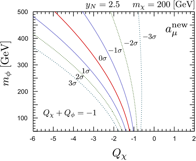
Figure 2: New physics contribution to muon g-2 (aμnewsuperscriptsubscript𝑎𝜇newa_{\mu}^{\rm new}) as a function of Qχsubscript𝑄𝜒Q_{\chi} and mϕsubscript𝑚italic-ϕm_{\phi}. Here we take yN=2.5subscript𝑦𝑁2.5y_{N}=2.5 and mχ=200subscript𝑚𝜒200m_{\chi}=200 GeV. We show contours for (aμnew/1010)=2.1,10.1,18.1,26.1,34.1,42.1superscriptsubscript𝑎𝜇newsuperscript10102.110.118.126.134.142.1(a_{\mu}^{\rm new}/10^{-10})=2.1,~{}10.1,~{}18.1,~{}26.1,~{}34.1,~{}42.1 and 50.150.150.1, from right to left, corresponding to 3σ,2σ,1σ,0σ,1σ,2σ3𝜎2𝜎1𝜎0𝜎1𝜎2𝜎-3\sigma,~{}-2\sigma,~{}-1\sigma,~{}0\sigma,~{}1\sigma,~{}2\sigma and 3σ3𝜎3\sigma deviation from the measured value, respectively.

In Fig. 2, we show the contribution to aμnewsuperscriptsubscript𝑎𝜇newa_{\mu}^{\rm new} as a function of Qχsubscript𝑄𝜒Q_{\chi} and mϕsubscript𝑚italic-ϕm_{\phi}. Here we take yN=2.5subscript𝑦𝑁2.5y_{N}=2.5 and mχ=200subscript𝑚𝜒200m_{\chi}=200 GeV. We show contours for (aμnew/1010)=2.1,10.1,18.1,26.1,34.1,42.1superscriptsubscript𝑎𝜇newsuperscript10102.110.118.126.134.142.1(a_{\mu}^{\rm new}/10^{-10})=2.1,~{}10.1,~{}18.1,~{}26.1,~{}34.1,~{}42.1 and 50.150.150.1, from right to left, corresponding to 3σ,2σ,1σ,0σ,1σ,2σ3𝜎2𝜎1𝜎0𝜎1𝜎2𝜎-3\sigma,~{}-2\sigma,~{}-1\sigma,~{}0\sigma,~{}1\sigma,~{}2\sigma and 3σ3𝜎3\sigma deviation from the measured value, respectively. We note that yNsubscript𝑦𝑁y_{N} dependence of aμnewsuperscriptsubscript𝑎𝜇newa_{\mu}^{\rm new} is trivial, that is, aμnewsuperscriptsubscript𝑎𝜇newa_{\mu}^{\rm new} is proportional to yN2superscriptsubscript𝑦𝑁2y_{N}^{2}, as shown in Eq. (2.3). For example, if one takes yN=1subscript𝑦𝑁1y_{N}=1, the values of aμnewsuperscriptsubscript𝑎𝜇newa_{\mu}^{\rm new} in Fig. 2 reduce by a factor (1/2.5)2=0.16superscript12.520.16(1/2.5)^{2}=0.16.

One can see that the region with Qχ>1subscript𝑄𝜒1Q_{\chi}>-1 (which corresponds to Qϕ<0subscript𝑄italic-ϕ0Q_{\phi}<0) is disfavored by the data of muon g-2. It is interesting to notice that the neutral fermion (Qχ=0subscript𝑄𝜒0Q_{\chi}=0, corresponding to Qϕ=1subscript𝑄italic-ϕ1Q_{\phi}=-1) is difficult to explain the anomaly in any values of mϕsubscript𝑚italic-ϕm_{\phi}, and on the other hand, the neutral scalar (Qϕ=0subscript𝑄italic-ϕ0Q_{\phi}=0, corresponding to Qχ=1subscript𝑄𝜒1Q_{\chi}=-1) can potentially accommodate the anomaly if the scalar ϕitalic-ϕ\phi is not so heavy. It is also interesting to note that the multi-charged fermion and scalar (such as Qχ=2,3,subscript𝑄𝜒23Q_{\chi}=-2,~{}-3,\cdots, corresponding to Qϕ=1,2,subscript𝑄italic-ϕ12Q_{\phi}=1,~{}2,\cdots) are also favored by the muon g-2 anomaly if mϕsubscript𝑚italic-ϕm_{\phi} is a right value for the anomaly. Therefore, the anomaly of muon g-2 constrains the QED charges as well as the mass scale of new particles.
Refer to caption Refer to caption

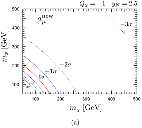
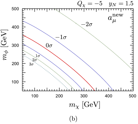
Figure 3: New physics contribution to muon g-2 (aμnewsuperscriptsubscript𝑎𝜇newa_{\mu}^{\rm new}) as a function of mχsubscript𝑚𝜒m_{\chi} and mϕsubscript𝑚italic-ϕm_{\phi} for (a) Qχ=1subscript𝑄𝜒1Q_{\chi}=-1 and and yN=2.5subscript𝑦𝑁2.5y_{N}=2.5 (b) Qχ=5subscript𝑄𝜒5Q_{\chi}=-5 and yN=1.5subscript𝑦𝑁1.5y_{N}=1.5, respectively. Contours for (aμnew/1010)=2.1,10.1,18.1,26.1,34.1,42.1superscriptsubscript𝑎𝜇newsuperscript10102.110.118.126.134.142.1(a_{\mu}^{\rm new}/10^{-10})=2.1,~{}10.1,~{}18.1,~{}26.1,~{}34.1,~{}42.1 and 50.150.150.1 (corresponding to 3σ,2σ,1σ,0σ,1σ,2σ3𝜎2𝜎1𝜎0𝜎1𝜎2𝜎-3\sigma,~{}-2\sigma,~{}-1\sigma,~{}0\sigma,~{}1\sigma,~{}2\sigma and 3σ3𝜎3\sigma deviation from the measured value) are shown, similar to Fig. 2.

In Fig. 3, we show aμnewsuperscriptsubscript𝑎𝜇newa_{\mu}^{\rm new} as a function of mχsubscript𝑚𝜒m_{\chi} and mϕsubscript𝑚italic-ϕm_{\phi} for (a) Qχ=1subscript𝑄𝜒1Q_{\chi}=-1 (correspondingtoQϕ=0)correspondingtosubscript𝑄italic-ϕ0({\rm corresponding~{}to}~{}Q_{\phi}=0) and yN=2.5subscript𝑦𝑁2.5y_{N}=2.5 and (b) Qχ=5subscript𝑄𝜒5Q_{\chi}=-5 (correspondingtoQϕ=4)correspondingtosubscript𝑄italic-ϕ4({\rm corresponding~{}to}~{}Q_{\phi}=4) and yN=1.5subscript𝑦𝑁1.5y_{N}=1.5. Contours for (aμnew/1010)=2.1,10.1,18.1,26.1,34.1,42.1superscriptsubscript𝑎𝜇newsuperscript10102.110.118.126.134.142.1(a_{\mu}^{\rm new}/10^{-10})=2.1,~{}10.1,~{}18.1,~{}26.1,~{}34.1,~{}42.1 and 50.150.150.1 (corresponding to 3σ,2σ,1σ,0σ,1σ,2σ3𝜎2𝜎1𝜎0𝜎1𝜎2𝜎-3\sigma,~{}-2\sigma,~{}-1\sigma,~{}0\sigma,~{}1\sigma,~{}2\sigma and 3σ3𝜎3\sigma deviation from the measured value) are shown, similar to Fig. 2.#2#2#2 If one changes the value of Yukawa coupling yNsubscript𝑦𝑁y_{N}, one should simply multiply the value of aμnewsuperscriptsubscript𝑎𝜇newa_{\mu}^{\rm new} in Fig. 3 (a) and (b) by a factor (yN2.5)2superscriptsubscript𝑦𝑁2.52(\frac{y_{N}}{2.5})^{2} and (yN1.5)2superscriptsubscript𝑦𝑁1.52(\frac{y_{N}}{1.5})^{2}, respectively. As one can see, new particles with their masses of about 100100100 GeV and the coupling yNO(1)similar-tosubscript𝑦𝑁𝑂1y_{N}\sim O(1) are strongly favored by the anomaly of muon g-2 when Qχ=1subscript𝑄𝜒1Q_{\chi}=-1. When the QED charge of χ𝜒\chi decreases further negatively (from 11-1 to 55-5), the muon g-2 gets larger even if the Yukawa coupling yNsubscript𝑦𝑁y_{N} gets smaller, as shown in Fig. 3 (b).

Since the anomaly of muon g-2 requires relatively light new particles (O(100GeV)similar-toabsent𝑂100GeV\sim O(100~{}{\rm GeV})) and/or relatively large Yukawa coupling (O(1)similar-toabsent𝑂1\sim O(1)) in this scenario, the EW precision observables can be affected by these new particles and new interactions. Therefore, we will check the effects of these particles on the EW observables in a next section.

We would also like to point out that the anomaly of muon g-2 suggests the existence of relatively light new particles and/or multi-charged particles. Therefore, it is very interesting to know whether these particles can be found directly or indirectly at the LHC. We will study the direct productions of these particles and the effects on Higgs decay to γγ𝛾𝛾\gamma\gamma at the LHC in a later section.

2.2 Model where both right- and left-handed muons have new Yukawa couplings

Unlike the previous case, here we consider that both right- and left-handed muons have new Yukawa interactions:

\displaystyle{\cal L} =\displaystyle= yLL¯2ΦχRyRμ¯RϕχLmχχ¯LχR+h.c.,formulae-sequencesubscript𝑦𝐿subscript¯𝐿2Φsubscript𝜒𝑅subscript𝑦𝑅subscript¯𝜇𝑅italic-ϕsubscript𝜒𝐿subscript𝑚𝜒subscript¯𝜒𝐿subscript𝜒𝑅hc\displaystyle-y_{L}\bar{L}_{2}\Phi\chi_{R}-y_{R}\bar{\mu}_{R}\phi\chi_{L}-m_{\chi}\bar{\chi}_{L}\chi_{R}+{\rm h.c.}, (2.6)

where L2(=(νμL,μL)T)annotatedsubscript𝐿2absentsuperscriptsubscript𝜈𝜇𝐿subscript𝜇𝐿TL_{2}~{}(=(\nu_{\mu L},~{}\mu_{L})^{\rm T}), Φ(=(ϕ1,ϕ2)T)annotatedΦabsentsuperscriptsubscriptitalic-ϕ1subscriptitalic-ϕ2T\Phi~{}(=(\phi_{1},\phi_{2})^{\rm T}) and ϕitalic-ϕ\phi are the second generation SU(2) doublet lepton, SU(2) doublet and singlet scalars, respectively, and χ𝜒\chi is SU(2) singlet fermion, whose mass is mχsubscript𝑚𝜒m_{\chi}. Here we have assumed the Z2subscript𝑍2Z_{2} parity again in order to simplify the model. Under the Z2subscript𝑍2Z_{2} parity, the SM particles are even, and new particles ϕitalic-ϕ\phi, ΦΦ\Phi and χ𝜒\chi are odd. We also implicitly assume the approximate muon flavor symmetry, under which χ𝜒\chi or (ϕ,Φitalic-ϕΦ\phi,~{}\Phi) has muon flavor number, so that the flavor mixing of this type of new Yukawa couplings are strongly suppressed. The model we discuss in this paper may be a part of the complete model. However, we think this part of the complete model is crucial for the muon g-2.#3#3#3In summary, we briefly comment on the possible completions of this type of model.

The QED charges of new particles are represented in term of QED charge of χ𝜒\chi field (Qχsubscript𝑄𝜒Q_{\chi}) as follows:

Q(ϕ1)𝑄subscriptitalic-ϕ1\displaystyle Q(\phi_{1}) \displaystyle\equiv Q1=Qχ,subscript𝑄1subscript𝑄𝜒\displaystyle Q_{1}=-Q_{\chi}, (2.7)
Q(ϕ2)𝑄subscriptitalic-ϕ2\displaystyle Q(\phi_{2}) \displaystyle\equiv Q2=1Qχ,subscript𝑄21subscript𝑄𝜒\displaystyle Q_{2}=-1-Q_{\chi}, (2.8)
Qϕsubscript𝑄italic-ϕ\displaystyle Q_{\phi} =\displaystyle= 1Qχ=Q2.1subscript𝑄𝜒subscript𝑄2\displaystyle-1-Q_{\chi}=Q_{2}. (2.9)

Since Qϕ=Q2subscript𝑄italic-ϕsubscript𝑄2Q_{\phi}=Q_{2}, ϕitalic-ϕ\phi and ϕ2subscriptitalic-ϕ2\phi_{2} can mix each other. For example, the following gauge invariant term induces the ϕ2ϕsubscriptitalic-ϕ2italic-ϕ\phi_{2}-\phi mixing mass terms after the electroweak symmetry is spontaneously broken:

=λM(HΦϕ)+h.c.=λMv2ϕ2ϕ+,\displaystyle{\cal L}=-\lambda M(H^{\dagger}\Phi\phi^{\dagger})+{\rm h.c.}=-\frac{\lambda Mv}{\sqrt{2}}\phi_{2}\phi^{\dagger}+\cdots, (2.10)

Here we parameterize the mass terms for ϕitalic-ϕ\phi and ϕ2subscriptitalic-ϕ2\phi_{2} as follows: #4#4#4When Qϕ=0subscript𝑄italic-ϕ0Q_{\phi}=0, mass term such as m2ϕϕ2superscript𝑚2italic-ϕsubscriptitalic-ϕ2-m^{2}\phi\phi_{2} is also possible. Here we neglect such a mass term for simplicity. Even if we include such a mass term, our result does not change qualitatively.

=(ϕ,ϕ2)(m112m122m122m222)(ϕϕ2).superscriptitalic-ϕsuperscriptsubscriptitalic-ϕ2subscriptsuperscript𝑚211subscriptsuperscript𝑚212subscriptsuperscript𝑚212subscriptsuperscript𝑚222italic-ϕsubscriptitalic-ϕ2\displaystyle{\cal L}=-\left(\phi^{\dagger},~{}\phi_{2}^{\dagger}\right)\left(\begin{array}[]{cc}m^{2}_{11}&m^{2}_{12}\\ m^{2}_{12}&m^{2}_{22}\end{array}\right)\left(\begin{array}[]{c}\phi\\ \phi_{2}\end{array}\right). (2.15)

Thus diagonalizing this mass matrix, we define the mass eigenstates si(i=1,2)subscript𝑠𝑖𝑖12s_{i}~{}(i=1,2) as

(ϕϕ2)i=Vijsj.subscriptitalic-ϕsubscriptitalic-ϕ2𝑖subscript𝑉𝑖𝑗subscript𝑠𝑗\displaystyle\left(\begin{array}[]{c}\phi\\ \phi_{2}\end{array}\right)_{i}=V_{ij}s_{j}. (2.18)

Here Vijsubscript𝑉𝑖𝑗V_{ij} is a mixing unitary matrix, which diagonalizes the mass matrix shown in Eq. (2.15). The mass eigen values are taken to be ms1<ms2subscript𝑚subscript𝑠1subscript𝑚subscript𝑠2m_{s_{1}}<m_{s_{2}}. This type of mixing terms are important to induce large contribution to muon g-2. The contributions to muon g-2 are summarized by

aμnewsuperscriptsubscript𝑎𝜇new\displaystyle a_{\mu}^{\rm new} =\displaystyle= Qχmμ216π2i{(yL2|V2i|2+yR2|V1i|2)(C11+C21)(si,χ,χ;p,q)\displaystyle-\frac{Q_{\chi}m_{\mu}^{2}}{16\pi^{2}}\sum_{i}\left\{\left(y_{L}^{2}|V_{2i}|^{2}+y_{R}^{2}|V_{1i}|^{2}\right)(C_{11}+C_{21})(s_{i},\chi,\chi;p,-q)\right. (2.19)
+2yLyRmχmμRe(V2iV1i)C11(si,χ,χ;p,q)}\displaystyle\left.\hskip 113.81102pt+2y_{L}y_{R}\frac{m_{\chi}}{m_{\mu}}{\rm Re}(V_{2i}V_{1i}^{*})C_{11}(s_{i},\chi,\chi;p,-q)\right\}
+\displaystyle+ Q2mμ216π2i{(yL2|V2i|2+yR2|V1i|2)(C12+C22)(si,si,χ;q,pq)\displaystyle\frac{Q_{2}m_{\mu}^{2}}{16\pi^{2}}\sum_{i}\left\{\left(y_{L}^{2}|V_{2i}|^{2}+y_{R}^{2}|V_{1i}|^{2}\right)(C_{12}+C_{22})(s_{i},s_{i},\chi;q,p-q)\right.
+2yLyRmχmμRe(V2iV1i)C12(si,si,χ;q,pq)},\displaystyle\left.\hskip 113.81102pt+2y_{L}y_{R}\frac{m_{\chi}}{m_{\mu}}{\rm Re}(V_{2i}V_{1i}^{*})C_{12}(s_{i},s_{i},\chi;q,p-q)\right\},

where p𝑝p and pq𝑝𝑞p-q are momenta of external muons, and q𝑞q is a photon momentum and a limit q20superscript𝑞20q^{2}\rightarrow 0 is taken. Here we show the explicit expressions of above Passarino-Veltman functions:

(C11+C21)(si,χ,χ;p,q)subscript𝐶11subscript𝐶21subscript𝑠𝑖𝜒𝜒𝑝𝑞\displaystyle(C_{11}+C_{21})(s_{i},\chi,\chi;p,-q) =\displaystyle= 1msi22+3yi6yi2+yi3+6yilnyi6(1yi)4,1subscriptsuperscript𝑚2subscript𝑠𝑖23subscript𝑦𝑖6superscriptsubscript𝑦𝑖2superscriptsubscript𝑦𝑖36subscript𝑦𝑖subscript𝑦𝑖6superscript1subscript𝑦𝑖4\displaystyle\frac{1}{m^{2}_{s_{i}}}\frac{2+3y_{i}-6y_{i}^{2}+y_{i}^{3}+6y_{i}\ln y_{i}}{6(1-y_{i})^{4}}, (2.20)
C11(si,χ,χ;p,q)subscript𝐶11subscript𝑠𝑖𝜒𝜒𝑝𝑞\displaystyle C_{11}(s_{i},\chi,\chi;p,-q) =\displaystyle= 1msi234yi+yi2+2lnyi2(1yi)3,1subscriptsuperscript𝑚2subscript𝑠𝑖34subscript𝑦𝑖superscriptsubscript𝑦𝑖22subscript𝑦𝑖2superscript1subscript𝑦𝑖3\displaystyle-\frac{1}{m^{2}_{s_{i}}}\frac{3-4y_{i}+y_{i}^{2}+2\ln y_{i}}{2(1-y_{i})^{3}}, (2.21)
(C22+C12)(si,si,χ;q,pq)subscript𝐶22subscript𝐶12subscript𝑠𝑖subscript𝑠𝑖𝜒𝑞𝑝𝑞\displaystyle(C_{22}+C_{12})(s_{i},s_{i},\chi;q,p-q) =\displaystyle= 1msi216yi+3yi2+2yi36yi2lnyi6(1yi)4,1subscriptsuperscript𝑚2subscript𝑠𝑖16subscript𝑦𝑖3superscriptsubscript𝑦𝑖22superscriptsubscript𝑦𝑖36superscriptsubscript𝑦𝑖2subscript𝑦𝑖6superscript1subscript𝑦𝑖4\displaystyle\frac{1}{m^{2}_{s_{i}}}\frac{1-6y_{i}+3y_{i}^{2}+2y_{i}^{3}-6y_{i}^{2}\ln y_{i}}{6(1-y_{i})^{4}}, (2.22)
C12(si,si,χ;q,pq)subscript𝐶12subscript𝑠𝑖subscript𝑠𝑖𝜒𝑞𝑝𝑞\displaystyle C_{12}(s_{i},s_{i},\chi;q,p-q) =\displaystyle= 1msi21yi2+2yilnyi2(1yi)3,1subscriptsuperscript𝑚2subscript𝑠𝑖1superscriptsubscript𝑦𝑖22subscript𝑦𝑖subscript𝑦𝑖2superscript1subscript𝑦𝑖3\displaystyle\frac{1}{m^{2}_{s_{i}}}\frac{1-y_{i}^{2}+2y_{i}\ln y_{i}}{2(1-y_{i})^{3}}, (2.23)

where yi=mχ2/msi2subscript𝑦𝑖subscriptsuperscript𝑚2𝜒subscriptsuperscript𝑚2subscript𝑠𝑖y_{i}=m^{2}_{\chi}/m^{2}_{s_{i}} and we neglected the higher order of O(mμ2/msi2)𝑂subscriptsuperscript𝑚2𝜇subscriptsuperscript𝑚2subscript𝑠𝑖O(m^{2}_{\mu}/m^{2}_{s_{i}}).

The effective operator which expresses the muon g-2 is written by

=vΛ2μRσμνμLFμν+h.c.,formulae-sequence𝑣superscriptΛ2subscript𝜇𝑅superscript𝜎𝜇𝜈subscript𝜇𝐿subscript𝐹𝜇𝜈hc\displaystyle{\cal L}=\frac{v}{\Lambda^{2}}\mu_{R}\sigma^{\mu\nu}\mu_{L}F_{\mu\nu}+{\rm h.c.}, (2.24)

where v𝑣v is a vacuum expectation value of Higgs boson, and Fμνsubscript𝐹𝜇𝜈F_{\mu\nu} is a field strength of photon field, and ΛΛ\Lambda is a typical scale related to new physics. As one see, the chirality of muon has to flip in this interaction. In the case where only right-handed muon has the new Yukawa interaction, the chirality flipping of muon happens in the external muon line in the loop diagram. On the other hands, in the present case where both right- and left-handed muons have the new Yukawa interactions, the chirality flipping can occur in the internal fermion line, which is proportional to the mass of the fermion χ𝜒\chi. That is why there are terms which are proportional to yRyLmχ/mμsubscript𝑦𝑅subscript𝑦𝐿subscript𝑚𝜒subscript𝑚𝜇y_{R}y_{L}m_{\chi}/m_{\mu} in Eq. (2.19). This contribution enhances the effects of muon g-2. Therefore, it is very important to explain the anomaly of muon g-2.
Refer to caption Refer to caption

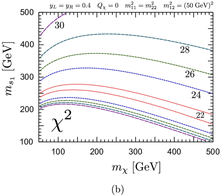
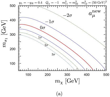
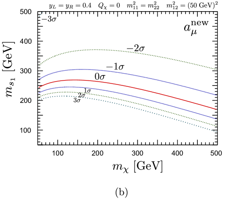
Figure 4: New physics contribution to muon g-2 (aμnewsuperscriptsubscript𝑎𝜇newa_{\mu}^{\rm new}) as a function of mχsubscript𝑚𝜒m_{\chi} and ms1subscript𝑚subscript𝑠1m_{s_{1}} in case of (a) Qχ=1subscript𝑄𝜒1Q_{\chi}=-1 and (b) Qχ=0subscript𝑄𝜒0Q_{\chi}=0. Contours for (aμnew/1010)=2.1,10.1,18.1,26.1,34.1,42.1superscriptsubscript𝑎𝜇newsuperscript10102.110.118.126.134.142.1(a_{\mu}^{\rm new}/10^{-10})=2.1,~{}10.1,~{}18.1,~{}26.1,~{}34.1,~{}42.1 and 50.150.150.1 (corresponding to 3σ,2σ,1σ,0σ,1σ,2σ3𝜎2𝜎1𝜎0𝜎1𝜎2𝜎-3\sigma,~{}-2\sigma,~{}-1\sigma,~{}0\sigma,~{}1\sigma,~{}2\sigma and 3σ3𝜎3\sigma deviation from the measured value) are shown. Here we assume that m112=m222superscriptsubscript𝑚112superscriptsubscript𝑚222m_{11}^{2}=m_{22}^{2}, m122=(50GeV)2superscriptsubscript𝑚122superscript50GeV2m_{12}^{2}=(50~{}{\rm GeV})^{2}. We also take (a) yL=yR=0.4subscript𝑦𝐿subscript𝑦𝑅0.4y_{L}=-y_{R}=0.4 and (b) yL=yR=0.4subscript𝑦𝐿subscript𝑦𝑅0.4y_{L}=y_{R}=0.4.

In Fig. 4, we show aμnewsuperscriptsubscript𝑎𝜇newa_{\mu}^{\rm new} as a function of mχsubscript𝑚𝜒m_{\chi} and ms1subscript𝑚subscript𝑠1m_{s_{1}} (which is a mass of lighter scalar state) in case of (a) Qχ=1subscript𝑄𝜒1Q_{\chi}=-1 and (b) Qχ=0subscript𝑄𝜒0Q_{\chi}=0. Contours for (aμnew/1010)=2.1superscriptsubscript𝑎𝜇newsuperscript10102.1(a_{\mu}^{\rm new}/10^{-10})=2.1, 10.1, 18.1, 26.1, 34.1, 42.1 and 50.1 (corresponding to 3σ,2σ,1σ,0σ,1σ,2σ3𝜎2𝜎1𝜎0𝜎1𝜎2𝜎-3\sigma,~{}-2\sigma,~{}-1\sigma,~{}0\sigma,~{}1\sigma,~{}2\sigma and 3σ3𝜎3\sigma deviation from the measured value) are shown. Here we took m112=m222subscriptsuperscript𝑚211subscriptsuperscript𝑚222m^{2}_{11}=m^{2}_{22}, m122=(50GeV)2superscriptsubscript𝑚122superscript50GeV2m_{12}^{2}=(50~{}{\rm GeV})^{2}, and (a) yL=yR=0.4subscript𝑦𝐿subscript𝑦𝑅0.4y_{L}=-y_{R}=0.4 (b) yL=yR=0.4subscript𝑦𝐿subscript𝑦𝑅0.4y_{L}=y_{R}=0.4. Note that in order to generate the positive contribution to muon g-2 in Fig. 4 (a), the sign of new Yukawa couplings had to be taken as yLyR<0subscript𝑦𝐿subscript𝑦𝑅0y_{L}y_{R}<0. On the other hand, in Fig. 4 (b), the sign of yLyRsubscript𝑦𝐿subscript𝑦𝑅y_{L}y_{R} should be positive. As shown in Fig. 4, compared to Fig. 3, even smaller Yukawa couplings and heavier new particles can accommodate the anomaly of muon g-2 because of the enhancement mentioned above. As can be seen from Fig. 4, when yLyRO(1)similar-tosubscript𝑦𝐿subscript𝑦𝑅similar-to𝑂1y_{L}\sim y_{R}\sim O(1), the EW scale new particles are expected in order to explain the anomaly of muon g-2. Therefore, we will analyze the effects on the EW precision observables and show the consistent region of parameters in a next section.

3 Effects on electroweak observables

In the previous section, we showed that the relatively light new particles are required in order to explain the anomaly of muon g-2. In addition, in the case where the only right-handed muon has new Yukawa interaction, the new Yukawa coupling should be relatively large for the anomaly of muon g-2. Therefore, we should check if the relatively light particles and the relatively large Yukawa coupling are consistent with the EW precision measurements. Although models which we consider in this paper may be only a part of complete models, we should know how these new particles affect EW observables.

In this section, we adopt the formalism in Refs.[10, 11, 12] in order to include the oblique corrections as well as the vertex corrections in the EW observables. First we briefly summarize the formalism [10, 11, 12].

In the presence of EW to TeV scale physics, it is well known that the oblique corrections in gauge boson self-energy are important. They are parameterized by Peskin-Takeuchi’s S, T, U parameters [13, 14, 15]:

αS4sW2cW2𝛼𝑆4superscriptsubscript𝑠𝑊2superscriptsubscript𝑐𝑊2\displaystyle\frac{\alpha S}{4s_{W}^{2}c_{W}^{2}} =\displaystyle= ΠZZ(MZ2)ΠZZ(0)MZ2c2WcWsWΠZγ(MZ2)MZ2Πγγ(MZ2)MZ2,subscriptΠ𝑍𝑍superscriptsubscript𝑀𝑍2subscriptΠ𝑍𝑍0superscriptsubscript𝑀𝑍2subscript𝑐2𝑊subscript𝑐𝑊subscript𝑠𝑊subscriptΠ𝑍𝛾superscriptsubscript𝑀𝑍2superscriptsubscript𝑀𝑍2subscriptΠ𝛾𝛾superscriptsubscript𝑀𝑍2superscriptsubscript𝑀𝑍2\displaystyle\frac{\Pi_{ZZ}(M_{Z}^{2})-\Pi_{ZZ}(0)}{M_{Z}^{2}}-\frac{c_{2W}}{c_{W}s_{W}}\frac{\Pi_{Z\gamma}(M_{Z}^{2})}{M_{Z}^{2}}-\frac{\Pi_{\gamma\gamma}(M_{Z}^{2})}{M_{Z}^{2}}, (3.25)
αT𝛼𝑇\displaystyle\alpha T =\displaystyle= ΠWW(0)MW2ΠZZ(0)MZ2,subscriptΠ𝑊𝑊0superscriptsubscript𝑀𝑊2subscriptΠ𝑍𝑍0superscriptsubscript𝑀𝑍2\displaystyle\frac{\Pi_{WW}(0)}{M_{W}^{2}}-\frac{\Pi_{ZZ}(0)}{M_{Z}^{2}}, (3.26)
αU4sW2𝛼𝑈4superscriptsubscript𝑠𝑊2\displaystyle\frac{\alpha U}{4s_{W}^{2}} =\displaystyle= ΠWW(MW2)ΠWW(0)MW2cW2ΠZZ(MZ2)ΠZZ(0)MZ2subscriptΠ𝑊𝑊superscriptsubscript𝑀𝑊2subscriptΠ𝑊𝑊0superscriptsubscript𝑀𝑊2superscriptsubscript𝑐𝑊2subscriptΠ𝑍𝑍superscriptsubscript𝑀𝑍2subscriptΠ𝑍𝑍0superscriptsubscript𝑀𝑍2\displaystyle\frac{\Pi_{WW}(M_{W}^{2})-\Pi_{WW}(0)}{M_{W}^{2}}-c_{W}^{2}\frac{\Pi_{ZZ}(M_{Z}^{2})-\Pi_{ZZ}(0)}{M_{Z}^{2}} (3.27)
2sWcWΠZγ(MZ2)MZ2sW2Πγγ(MZ2)MZ2.2subscript𝑠𝑊subscript𝑐𝑊subscriptΠ𝑍𝛾superscriptsubscript𝑀𝑍2superscriptsubscript𝑀𝑍2superscriptsubscript𝑠𝑊2subscriptΠ𝛾𝛾superscriptsubscript𝑀𝑍2superscriptsubscript𝑀𝑍2\displaystyle-2s_{W}c_{W}\frac{\Pi_{Z\gamma}(M_{Z}^{2})}{M_{Z}^{2}}-s_{W}^{2}\frac{\Pi_{\gamma\gamma}(M_{Z}^{2})}{M_{Z}^{2}}.

Here we use the notation cWsubscript𝑐𝑊c_{W} and sWsubscript𝑠𝑊s_{W} to refer to the cosine and sine of the weak mixing angle and c2W=cW2sW2subscript𝑐2𝑊superscriptsubscript𝑐𝑊2superscriptsubscript𝑠𝑊2c_{2W}=c_{W}^{2}-s_{W}^{2}. In addition, in Refs.[10, 11], RZsubscript𝑅𝑍R_{Z} and RWsubscript𝑅𝑊R_{W} parameters are introduced in order to account for the smaller corrections:

αRZ4sW2cW2𝛼subscript𝑅𝑍4superscriptsubscript𝑠𝑊2superscriptsubscript𝑐𝑊2\displaystyle\frac{\alpha R_{Z}}{4s_{W}^{2}c_{W}^{2}} =\displaystyle= dΠZZ(p2)dp2|p2=MZ2ΠZZ(MZ2)ΠZZ(0)MZ2,evaluated-at𝑑subscriptΠ𝑍𝑍superscript𝑝2𝑑superscript𝑝2superscript𝑝2superscriptsubscript𝑀𝑍2subscriptΠ𝑍𝑍superscriptsubscript𝑀𝑍2subscriptΠ𝑍𝑍0superscriptsubscript𝑀𝑍2\displaystyle\left.\frac{d\Pi_{ZZ}(p^{2})}{dp^{2}}\right|_{p^{2}=M_{Z}^{2}}-\frac{\Pi_{ZZ}(M_{Z}^{2})-\Pi_{ZZ}(0)}{M_{Z}^{2}}, (3.28)
αRW4sW2𝛼subscript𝑅𝑊4superscriptsubscript𝑠𝑊2\displaystyle\frac{\alpha R_{W}}{4s_{W}^{2}} =\displaystyle= ΠWW(MZ2)ΠWW(MW2)MZ2MW2ΠWW(MW2)ΠWW(0)MW2.subscriptΠ𝑊𝑊superscriptsubscript𝑀𝑍2subscriptΠ𝑊𝑊superscriptsubscript𝑀𝑊2superscriptsubscript𝑀𝑍2superscriptsubscript𝑀𝑊2subscriptΠ𝑊𝑊superscriptsubscript𝑀𝑊2subscriptΠ𝑊𝑊0superscriptsubscript𝑀𝑊2\displaystyle\frac{\Pi_{WW}(M_{Z}^{2})-\Pi_{WW}(M_{W}^{2})}{M_{Z}^{2}-M_{W}^{2}}-\frac{\Pi_{WW}(M_{W}^{2})-\Pi_{WW}(0)}{M_{W}^{2}}. (3.29)

Furthermore, new particles have effects on the running QED coupling constant α(MZ2)𝛼superscriptsubscript𝑀𝑍2\alpha(M_{Z}^{2}) [3, 12]:

α(MZ2)=α1Δαlep(MZ2)Δαhad(5)(MZ2)Δαtop(MZ2)Δαnew(MZ2)𝛼superscriptsubscript𝑀𝑍2𝛼1Δsubscript𝛼lepsuperscriptsubscript𝑀𝑍2Δsuperscriptsubscript𝛼had5superscriptsubscript𝑀𝑍2Δsubscript𝛼topsuperscriptsubscript𝑀𝑍2Δsubscript𝛼newsuperscriptsubscript𝑀𝑍2\displaystyle\alpha(M_{Z}^{2})=\frac{\alpha}{1-\Delta\alpha_{\rm lep}(M_{Z}^{2})-\Delta\alpha_{\rm had}^{(5)}(M_{Z}^{2})-\Delta\alpha_{\rm top}(M_{Z}^{2})-\Delta\alpha_{\rm new}(M_{Z}^{2})} (3.30)

Here Δαlep(MZ2)Δsubscript𝛼lepsuperscriptsubscript𝑀𝑍2\Delta\alpha_{\rm lep}(M_{Z}^{2}), Δαhad(5)(MZ2)Δsuperscriptsubscript𝛼had5superscriptsubscript𝑀𝑍2\Delta\alpha_{\rm had}^{(5)}(M_{Z}^{2}), Δαtop(MZ2)Δsubscript𝛼topsuperscriptsubscript𝑀𝑍2\Delta\alpha_{\rm top}(M_{Z}^{2}), and Δαnew(MZ2)Δsubscript𝛼newsuperscriptsubscript𝑀𝑍2\Delta\alpha_{\rm new}(M_{Z}^{2}) are the leptonic, the five-flavor hadronic, the top quark and the new physics contributions to the running of the QED coupling constant respectively. The new physics contributions to the running of the QED coupling constant Δαnew(MZ2)Δsubscript𝛼newsuperscriptsubscript𝑀𝑍2\Delta\alpha_{\rm new}(M_{Z}^{2}) are defined as

Δαnew(MZ2)=Πγγ(MZ2)MZ2Πγγ(p2)p2|p2=0Δsubscript𝛼newsuperscriptsubscript𝑀𝑍2subscriptΠ𝛾𝛾superscriptsubscript𝑀𝑍2superscriptsubscript𝑀𝑍2evaluated-atsubscriptΠ𝛾𝛾superscript𝑝2superscript𝑝2superscript𝑝20\displaystyle\Delta\alpha_{\rm new}(M_{Z}^{2})=\left.\frac{\Pi_{\gamma\gamma}(M_{Z}^{2})}{M_{Z}^{2}}-\frac{\Pi_{\gamma\gamma}(p^{2})}{p^{2}}\right|_{p^{2}=0} (3.31)

These oblique parameters contribute to EW observables, as shown in Refs. [10, 11, 12].

If muon has O(1)𝑂1O(1) new Yukawa couplings,#5#5#5In this paper, we assume that electron and tau do not have O(1)𝑂1O(1) extra Yukawa couplings, for simplicity. it induces non-universal vertex corrections to the Zμ+μ𝑍superscript𝜇superscript𝜇Z\mu^{+}\mu^{-} coupling. The standard model coupling of Zμ+μ𝑍superscript𝜇superscript𝜇Z\mu^{+}\mu^{-} is given by

igcWγμ[gLSM,μPL+gRSM,μPR],𝑖𝑔subscript𝑐𝑊subscript𝛾𝜇delimited-[]subscriptsuperscript𝑔SM𝜇𝐿subscript𝑃𝐿subscriptsuperscript𝑔SM𝜇𝑅subscript𝑃𝑅\displaystyle i\frac{g}{c_{W}}\gamma_{\mu}[g^{\rm SM,\mu}_{L}P_{L}+g^{\rm SM,\mu}_{R}P_{R}], (3.32)

where gL,RSM,μsubscriptsuperscript𝑔SM𝜇𝐿𝑅g^{\rm SM,\mu}_{L,R} are the standard model couplings, and their tree level contributions are gLSM,μ=12+sW2superscriptsubscript𝑔𝐿SM𝜇12superscriptsubscript𝑠𝑊2g_{L}^{\rm SM,\mu}=-\frac{1}{2}+s_{W}^{2} and gRSM,μ=sW2superscriptsubscript𝑔𝑅SM𝜇superscriptsubscript𝑠𝑊2g_{R}^{\rm SM,\mu}=s_{W}^{2}. When we take into account of corrections to Zμ+μ𝑍superscript𝜇superscript𝜇Z\mu^{+}\mu^{-} vertex via the new Yukawa coupling (including the corresponding wave function renormalization), the Zμ+μ𝑍superscript𝜇superscript𝜇Z\mu^{+}\mu^{-} coupling is modified by

igcWγμ[(gLSM,μ+ΔgLμ)PL+(gRSM,μ+ΔgRμ)PR].𝑖𝑔subscript𝑐𝑊subscript𝛾𝜇delimited-[]subscriptsuperscript𝑔SM𝜇𝐿Δsuperscriptsubscript𝑔𝐿𝜇subscript𝑃𝐿subscriptsuperscript𝑔SM𝜇𝑅Δsuperscriptsubscript𝑔𝑅𝜇subscript𝑃𝑅\displaystyle i\frac{g}{c_{W}}\gamma_{\mu}\left[(g^{\rm SM,\mu}_{L}+\Delta g_{L}^{\mu})P_{L}+(g^{\rm SM,\mu}_{R}+\Delta g_{R}^{\mu})P_{R}\right]. (3.33)

Here the vertex corrections generated by new particles are parameterized by ΔgL,RμΔsubscriptsuperscript𝑔𝜇𝐿𝑅\Delta g^{\mu}_{L,R}.

The corrections to Wμνμ𝑊𝜇subscript𝜈𝜇W\mu\nu_{\mu} vertex generates the corrections to the Fermi constant GFsubscript𝐺𝐹G_{F} and therefore, we parameterize it as Δδ¯GΔsubscript¯𝛿𝐺\Delta\bar{\delta}_{G}. The Δδ¯GΔsubscript¯𝛿𝐺\Delta\bar{\delta}_{G} for the new physics contributions from the vertex and box diagrams to the μ𝜇\mu-decay process is defined as

GF=GFSM+ob.+g242MW2Δδ¯G.subscript𝐺𝐹superscriptsubscript𝐺𝐹SMobsuperscript𝑔242superscriptsubscript𝑀𝑊2Δsubscript¯𝛿𝐺\displaystyle G_{F}=G_{F}^{\rm SM+ob.}+\frac{g^{2}}{4\sqrt{2}M_{W}^{2}}\Delta\bar{\delta}_{G}. (3.34)

Here GFSM+ob.superscriptsubscript𝐺𝐹SMobG_{F}^{\rm SM+ob.} is the muon decay constant including effects of SM radiative corrections and new physics oblique corrections except the vertex and box corrections from new physics.

data SM fit pull Sample model pull
line-shape & FB asym.:
ΓZsubscriptΓ𝑍\Gamma_{Z}(GeV) 2.4952(23) 2.4954 -0.1 2.4963 -0.5
σh0superscriptsubscript𝜎0\sigma_{h}^{0} (nb) 41.541(37) 41.479 1.7 41.479 1.7
Resubscript𝑅𝑒R_{e} 20.804(50) 20.740 1.3 20.741 1.3
Rμsubscript𝑅𝜇R_{\mu} 20.785(33) 20.740 1.4 20.740 1.3
Rτsubscript𝑅𝜏R_{\tau} 20.764(45) 20.787 -0.5 20.788 -0.5
AFB0,esuperscriptsubscript𝐴FB0𝑒A_{\rm FB}^{0,e} 0.0145(25) 0.0163 -0.7 0.0163 -0.7
AFB0,μsuperscriptsubscript𝐴FB0𝜇A_{\rm FB}^{0,\mu} 0.0169(13) 0.0163 0.5 0.0163 0.4
AFB0,τsuperscriptsubscript𝐴FB0𝜏A_{\rm FB}^{0,\tau} 0.0188(17) 0.0163 1.5 0.0163 1.4
τ𝜏\tau polarization:
Aτsubscript𝐴𝜏A_{\tau} 0.1439(43) 0.1472 -0.8 0.1476 -0.9
Aesubscript𝐴𝑒A_{e} 0.1498(49) 0.1472 0.5 0.1476 0.4
b𝑏b and c𝑐c quark results:
Rbsubscript𝑅𝑏R_{b} 0.21629(66) 0.21579 0.8 0.21580 0.7
Rcsubscript𝑅𝑐R_{c} 0.1721(30) 0.1723 -0.1 0.1722 0.0
AFB0,bsuperscriptsubscript𝐴FB0𝑏A_{\rm FB}^{0,b} 0.0992(16) 0.1032 -2.5 0.1035 -2.7
AFB0,csuperscriptsubscript𝐴FB0𝑐A_{\rm FB}^{0,c} 0.0707(35) 0.0738 -0.9 0.0740 -0.9
Absubscript𝐴𝑏A_{b} 0.923(20) 0.935 -0.6 0.935 -0.6
Acsubscript𝐴𝑐A_{c} 0.670(27) 0.668 0.1 0.668 0.1
SLD results:
Aesubscript𝐴𝑒A_{e} 0.1516(21) 0.1472 2.1 0.1476 1.9
Aμsubscript𝐴𝜇A_{\mu} 0.142(15) 0.1472 -0.4 0.1476 -0.4
Aτsubscript𝐴𝜏A_{\tau} 0.136(15) 0.1472 -0.8 0.1476 -0.8
W mass and width:
MWsubscript𝑀𝑊M_{W} (GeV) 80.385(15)[16] 80.363 1.5 80.376 0.6
ΓWsubscriptΓ𝑊\Gamma_{W} (GeV) 2.085(42) 2.091 -0.1 2.092 -0.2
muon g-2:
aμnew(109)superscriptsubscript𝑎𝜇newsuperscript109a_{\mu}^{\rm new}(10^{-9}) 2.61(0.80) 0 3.3 3.15 -0.7
Input parameters
Δαhad(5)(MZ2)Δsuperscriptsubscript𝛼had5superscriptsubscript𝑀𝑍2\Delta\alpha_{\rm had}^{(5)}(M_{Z}^{2}) 0.027626(138) 0.027592 0.3 0.027626 0.0
αs(MZ)subscript𝛼𝑠subscript𝑀𝑍\alpha_{s}(M_{Z}) 0.1184(7) 0.1184 0.0 0.1184 0.0
mtsubscript𝑚𝑡m_{t} (GeV) 173.2(0.9)[17] 173.7 -0.6 173.3 -0.1
mhsubscript𝑚m_{h} (GeV) 125 125
yL=yRsubscript𝑦𝐿subscript𝑦𝑅y_{L}=y_{R}Qχsubscript𝑄𝜒Q_{\chi} - - - 0.4, 0
mϕ1subscript𝑚subscriptitalic-ϕ1m_{\phi_{1}}, mχsubscript𝑚𝜒m_{\chi} (GeV) - - - 300, 200
m112=m222superscriptsubscript𝑚112superscriptsubscript𝑚222m_{11}^{2}=m_{22}^{2}, m122superscriptsubscript𝑚122m_{12}^{2} (GeV)2superscriptGeV2({\rm GeV})^{2} - - - (250)2superscript2502(250)^{2}, (50)2superscript502(50)^{2}
χ2/(d.o.f)\chi^{2}/(d.o.f) 34.8/(22) 22.5/(15)
Table 1: Experimental data and theoretical predictions of electroweak observables. The predicted values of the SM and sample model discussed in Sec. 3.2 are shown.

Refer to caption Refer to caption

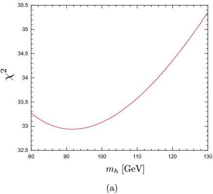
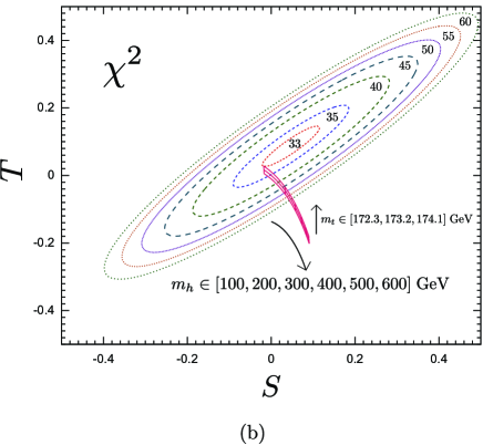
Figure 5: (a) χ2superscript𝜒2\chi^{2} of the EW observables listed in Table. 1 as a function of the Higgs boson mass mhsubscript𝑚m_{h} within the SM. (b) χ2superscript𝜒2\chi^{2} contours shown in dashed lines in S-T plane, assuming that other oblique corrections (U𝑈U, RWsubscript𝑅𝑊R_{W}, RZsubscript𝑅𝑍R_{Z}) and vertex corrections are zero. Reference Higgs boson mass and top quark mass are taken to be 125125125 GeV and 173.2 GeV, respectively. We also show the predicted S-T values (shown in solid lines) in the SM, varying the Higgs boson mass and top quark mass from the reference values.

Using the formalism in Ref.[10, 11], one can calculate EW observables listed in Table 1 without assuming lepton universality. First, we show a result of the SM fit of the EW observables in Fig. 5 (a) as a function of Higgs boson mass mhsubscript𝑚m_{h}. The best fit point is at mh=91subscript𝑚91m_{h}=91 GeV. This is consistent with the result shown by the LEP electroweak working group [18]. In Table 1, we show the SM fit when Higgs boson mass is assumed to be 125 GeV, which has been suggested by the latest LHC data. In Fig. 5(b), χ2superscript𝜒2\chi^{2} contours are shown in dashed lines in S-T plane. Here we assume that other oblique corrections (U𝑈U, RWsubscript𝑅𝑊R_{W}, RZsubscript𝑅𝑍R_{Z}) and vertex corrections are zero. Reference Higgs boson mass and top quark mass are taken to be 125 GeV, 173.2 GeV, respectively. The predicted values of S-T parameters are also shown by varying the Higgs boson mass and top quark mass from the reference values. We note that the SM fit with lighter Higgs boson is good except for the muon g-2, and small positive S and T (S0.05,T0.1(S\sim 0.05,~{}T\sim 0.1) can decrease the χ2superscript𝜒2\chi^{2} further. Therefore, we need new physics which largely contributes to muon g-2, but whose effects on other EW observables are small. In this section, we analyze the EW observables in models discussed in the previous section. In this analysis, we assume mh=125subscript𝑚125m_{h}=125 GeV.

3.1 Model with SU(2) singlet scalar (ϕitalic-ϕ\phi) and singlet Dirac fermion (χ𝜒\chi)

Since the new scalar ϕitalic-ϕ\phi and new fermion χ𝜒\chi are SU(2) singlet, they do not couple to W boson. But if it has a QED charge, it can couple to photon and Z boson. Here we list the corrections to self-energy functions of gauge bosons in this model.

The singlet fermion (χ𝜒\chi) contributions are given by

ΠWW(χ)(p2)superscriptsubscriptΠ𝑊𝑊𝜒superscript𝑝2\displaystyle\Pi_{WW}^{(\chi)}(p^{2}) =\displaystyle= 00\displaystyle 0
ΠZZ(χ)(p2)superscriptsubscriptΠ𝑍𝑍𝜒superscript𝑝2\displaystyle\Pi_{ZZ}^{(\chi)}(p^{2}) =\displaystyle= g2Qχ2sW44π2cW2[mχ2B0(χ,χ)p2{B1(χ,χ)+B21(χ,χ)}2(1ϵ)B22(χ,χ)],superscript𝑔2superscriptsubscript𝑄𝜒2superscriptsubscript𝑠𝑊44superscript𝜋2superscriptsubscript𝑐𝑊2delimited-[]superscriptsubscript𝑚𝜒2subscript𝐵0𝜒𝜒superscript𝑝2subscript𝐵1𝜒𝜒subscript𝐵21𝜒𝜒21italic-ϵsubscript𝐵22𝜒𝜒\displaystyle-\frac{g^{2}Q_{\chi}^{2}s_{W}^{4}}{4\pi^{2}c_{W}^{2}}\left[m_{\chi}^{2}B_{0}(\chi,\chi)-p^{2}\left\{B_{1}(\chi,\chi)+B_{21}(\chi,\chi)\right\}-2(1-\epsilon)B_{22}(\chi,\chi)\right],
Πγγ(χ)(p2)superscriptsubscriptΠ𝛾𝛾𝜒superscript𝑝2\displaystyle\Pi_{\gamma\gamma}^{(\chi)}(p^{2}) =\displaystyle= e24π2Qχ2[mχ2B0(χ,χ)p2{B1(χ,χ)+B21(χ,χ)}2(1ϵ)B22(χ,χ)],superscript𝑒24superscript𝜋2superscriptsubscript𝑄𝜒2delimited-[]subscriptsuperscript𝑚2𝜒subscript𝐵0𝜒𝜒superscript𝑝2subscript𝐵1𝜒𝜒subscript𝐵21𝜒𝜒21italic-ϵsubscript𝐵22𝜒𝜒\displaystyle-\frac{e^{2}}{4\pi^{2}}Q_{\chi}^{2}\left[m^{2}_{\chi}B_{0}(\chi,\chi)-p^{2}\left\{B_{1}(\chi,\chi)+B_{21}(\chi,\chi)\right\}-2(1-\epsilon)B_{22}(\chi,\chi)\right],
ΠγZ(χ)(p2)superscriptsubscriptΠ𝛾𝑍𝜒superscript𝑝2\displaystyle\Pi_{\gamma Z}^{(\chi)}(p^{2}) =\displaystyle= geQχ2sW24π2cW[mχ2B0(χ,χ)p2{B1(χ,χ)+B21(χ,χ)}2(1ϵ)B22(χ,χ)].𝑔𝑒superscriptsubscript𝑄𝜒2superscriptsubscript𝑠𝑊24superscript𝜋2subscript𝑐𝑊delimited-[]superscriptsubscript𝑚𝜒2subscript𝐵0𝜒𝜒superscript𝑝2subscript𝐵1𝜒𝜒subscript𝐵21𝜒𝜒21italic-ϵsubscript𝐵22𝜒𝜒\displaystyle\frac{geQ_{\chi}^{2}s_{W}^{2}}{4\pi^{2}c_{W}}\left[m_{\chi}^{2}B_{0}(\chi,\chi)-p^{2}\left\{B_{1}(\chi,\chi)+B_{21}(\chi,\chi)\right\}-2(1-\epsilon)B_{22}(\chi,\chi)\right].

Here BX(i,j)=BX(mi2,mj2;p)(X=0,1,21,22)subscript𝐵𝑋𝑖𝑗subscript𝐵𝑋superscriptsubscript𝑚𝑖2superscriptsubscript𝑚𝑗2𝑝𝑋012122B_{X}(i,j)=B_{X}(m_{i}^{2},m_{j}^{2};p)~{}(X=0,~{}1,~{}21,~{}22), which are Passarino-Veltman functions and are shown explicitly in Appendix. We use the dimensional regularization in space-time dimension D=42ϵ𝐷42italic-ϵD=4-2\epsilon.

The singlet scalar (ϕitalic-ϕ\phi) contributions are given by

ΠWW(ϕ)(p2)superscriptsubscriptΠ𝑊𝑊italic-ϕsuperscript𝑝2\displaystyle\Pi_{WW}^{(\phi)}(p^{2}) =\displaystyle= 00\displaystyle 0
ΠZZ(ϕ)(p2)superscriptsubscriptΠ𝑍𝑍italic-ϕsuperscript𝑝2\displaystyle\Pi_{ZZ}^{(\phi)}(p^{2}) =\displaystyle= g24π2cW2Qϕ2sW4{B22(ϕ,ϕ)12A(ϕ)},superscript𝑔24superscript𝜋2superscriptsubscript𝑐𝑊2superscriptsubscript𝑄italic-ϕ2superscriptsubscript𝑠𝑊4subscript𝐵22italic-ϕitalic-ϕ12𝐴italic-ϕ\displaystyle\frac{g^{2}}{4\pi^{2}c_{W}^{2}}Q_{\phi}^{2}s_{W}^{4}\left\{B_{22}(\phi,\phi)-\frac{1}{2}A(\phi)\right\},
Πγγ(ϕ)(p2)superscriptsubscriptΠ𝛾𝛾italic-ϕsuperscript𝑝2\displaystyle\Pi_{\gamma\gamma}^{(\phi)}(p^{2}) =\displaystyle= e24π2Qϕ2{B22(ϕ,ϕ)12A(ϕ)},superscript𝑒24superscript𝜋2superscriptsubscript𝑄italic-ϕ2subscript𝐵22italic-ϕitalic-ϕ12𝐴italic-ϕ\displaystyle\frac{e^{2}}{4\pi^{2}}Q_{\phi}^{2}\left\{B_{22}(\phi,\phi)-\frac{1}{2}A(\phi)\right\},
ΠγZ(ϕ)(p2)superscriptsubscriptΠ𝛾𝑍italic-ϕsuperscript𝑝2\displaystyle\Pi_{\gamma Z}^{(\phi)}(p^{2}) =\displaystyle= ge4π2cWQϕ2sW2{B22(ϕ,ϕ)12A(ϕ)}.𝑔𝑒4superscript𝜋2subscript𝑐𝑊superscriptsubscript𝑄italic-ϕ2superscriptsubscript𝑠𝑊2subscript𝐵22italic-ϕitalic-ϕ12𝐴italic-ϕ\displaystyle-\frac{ge}{4\pi^{2}c_{W}}Q_{\phi}^{2}s_{W}^{2}\left\{B_{22}(\phi,\phi)-\frac{1}{2}A(\phi)\right\}. (3.36)

Here Passarino-Veltman functions B22(i,j)(=B22(mi2,mj2;p))annotatedsubscript𝐵22𝑖𝑗absentsubscript𝐵22superscriptsubscript𝑚𝑖2superscriptsubscript𝑚𝑗2𝑝B_{22}(i,j)(=B_{22}(m_{i}^{2},m_{j}^{2};p)) and A(ϕ)𝐴italic-ϕA(\phi) are shown in Appendix. We can easily show that Peskin-Takeuchi STU parameters in this case vanish (S=T=U=0𝑆𝑇𝑈0S=T=U=0), since the new particles do not have SU(2)L interactions. Thus, the leading contributions to the oblique corrections are RZsubscript𝑅𝑍R_{Z} parameter and Δαnew(MZ2)Δsubscript𝛼newsuperscriptsubscript𝑀𝑍2\Delta\alpha_{\rm new}(M_{Z}^{2}):

RZsubscript𝑅𝑍\displaystyle R_{Z} =\displaystyle= 4sW4Qχ23π[1+6mχ2MZ2{14mχ2MZ24mχ2MZ21tan1[14mχ2MZ21]}]4superscriptsubscript𝑠𝑊4superscriptsubscript𝑄𝜒23𝜋delimited-[]16superscriptsubscript𝑚𝜒2superscriptsubscript𝑀𝑍214superscriptsubscript𝑚𝜒2superscriptsubscript𝑀𝑍24superscriptsubscript𝑚𝜒2superscriptsubscript𝑀𝑍21superscript114superscriptsubscript𝑚𝜒2superscriptsubscript𝑀𝑍21\displaystyle\frac{4s_{W}^{4}Q_{\chi}^{2}}{3\pi}\left[1+\frac{6m_{\chi}^{2}}{M_{Z}^{2}}\left\{1-\frac{\frac{4m_{\chi}^{2}}{M_{Z}^{2}}}{\sqrt{\frac{4m_{\chi}^{2}}{M_{Z}^{2}}-1}}\tan^{-1}\left[\frac{1}{\sqrt{\frac{4m_{\chi}^{2}}{M_{Z}^{2}}-1}}\right]\right\}\right] (3.37)
+sW4Qϕ23π[112mϕ2MZ2{14mϕ2MZ21tan1[14mϕ2MZ21]}],superscriptsubscript𝑠𝑊4superscriptsubscript𝑄italic-ϕ23𝜋delimited-[]112superscriptsubscript𝑚italic-ϕ2superscriptsubscript𝑀𝑍214superscriptsubscript𝑚italic-ϕ2superscriptsubscript𝑀𝑍21superscript114superscriptsubscript𝑚italic-ϕ2superscriptsubscript𝑀𝑍21\displaystyle+\frac{s_{W}^{4}Q_{\phi}^{2}}{3\pi}\left[1-\frac{12m_{\phi}^{2}}{M_{Z}^{2}}\left\{1-\sqrt{\frac{4m_{\phi}^{2}}{M_{Z}^{2}}-1}\tan^{-1}\left[\frac{1}{\sqrt{\frac{4m_{\phi}^{2}}{M_{Z}^{2}}-1}}\right]\right\}\right],
Δαnew(MZ2)Δsubscript𝛼newsuperscriptsubscript𝑀𝑍2\displaystyle\Delta\alpha_{\rm new}(M_{Z}^{2}) =\displaystyle= 5αQχ29π[1+12mχ25MZ265(1+2mχ2MZ2)4mχ2MZ21tan1[14mχ2MZ21]]5𝛼superscriptsubscript𝑄𝜒29𝜋delimited-[]112superscriptsubscript𝑚𝜒25superscriptsubscript𝑀𝑍26512superscriptsubscript𝑚𝜒2superscriptsubscript𝑀𝑍24superscriptsubscript𝑚𝜒2superscriptsubscript𝑀𝑍21superscript114superscriptsubscript𝑚𝜒2superscriptsubscript𝑀𝑍21\displaystyle-\frac{5\alpha Q_{\chi}^{2}}{9\pi}\left[1+\frac{12m_{\chi}^{2}}{5M_{Z}^{2}}-\frac{6}{5}\left(1+\frac{2m_{\chi}^{2}}{M_{Z}^{2}}\right)\sqrt{\frac{4m_{\chi}^{2}}{M_{Z}^{2}}-1}\tan^{-1}\left[\frac{1}{\sqrt{\frac{4m_{\chi}^{2}}{M_{Z}^{2}}-1}}\right]\right] (3.38)
2αQϕ29π[13mϕ2MZ2+344mϕ2MZ21tan1[14mϕ2MZ21]],2𝛼superscriptsubscript𝑄italic-ϕ29𝜋delimited-[]13superscriptsubscript𝑚italic-ϕ2superscriptsubscript𝑀𝑍2344superscriptsubscript𝑚italic-ϕ2superscriptsubscript𝑀𝑍21superscript114superscriptsubscript𝑚italic-ϕ2superscriptsubscript𝑀𝑍21\displaystyle-\frac{2\alpha Q_{\phi}^{2}}{9\pi}\left[1-\frac{3m_{\phi}^{2}}{M_{Z}^{2}}+\frac{3}{4}\sqrt{\frac{4m_{\phi}^{2}}{M_{Z}^{2}}-1}\tan^{-1}\left[\frac{1}{\sqrt{\frac{4m_{\phi}^{2}}{M_{Z}^{2}}-1}}\right]\right],

where we assume 2mχ>MZ2subscript𝑚𝜒subscript𝑀𝑍2m_{\chi}>M_{Z} and 2mϕ>MZ2subscript𝑚italic-ϕsubscript𝑀𝑍2m_{\phi}>M_{Z}.

As discussed in the previous section, in order to explain the anomaly of muon g-2, the new Yukawa coupling in this model should be relatively large. In this case, the potentially large vertex corrections may be expected, as shown in Fig.6.

Refer to caption

Figure 6: Feynman diagrams for vertex corrections to Zμ+μ𝑍superscript𝜇superscript𝜇Z\mu^{+}\mu^{-} coupling.

The results are expressed by

ΔgLμΔsuperscriptsubscript𝑔𝐿𝜇\displaystyle\Delta g_{L}^{\mu} =\displaystyle= 0,0\displaystyle 0, (3.39)
ΔgRμΔsuperscriptsubscript𝑔𝑅𝜇\displaystyle\Delta g_{R}^{\mu} =\displaystyle= yN216π2[2QϕsW2C24(ϕ,χ,ϕ;p,qp)\displaystyle\frac{y_{N}^{2}}{16\pi^{2}}\left[-2Q_{\phi}s_{W}^{2}C_{24}(\phi,\chi,\phi;p,q-p)\right. (3.40)
+QχsW2{122C24MZ2(C12+C23)+mχ2C0}(χ,ϕ,χ;qp,p)subscript𝑄𝜒superscriptsubscript𝑠𝑊2122subscript𝐶24superscriptsubscript𝑀𝑍2subscript𝐶12subscript𝐶23superscriptsubscript𝑚𝜒2subscript𝐶0𝜒italic-ϕ𝜒𝑞𝑝𝑝\displaystyle+Q_{\chi}s_{W}^{2}\left\{\frac{1}{2}-2C_{24}-M_{Z}^{2}(C_{12}+C_{23})+m_{\chi}^{2}C_{0}\right\}(\chi,\phi,\chi;q-p,p)
sW2(B0+B1)(ϕ,χ;p)],\displaystyle\left.-s_{W}^{2}(B_{0}+B_{1})(\phi,\chi;p)\right],

where p𝑝p, qp𝑞𝑝q-p and q𝑞q are muon, anti-muon and Z-boson momenta, respectively. Here Passarino-Veltman functions CX(X=0,12,23,24)subscript𝐶𝑋𝑋0122324C_{X}~{}(X=0,~{}12,~{}23,~{}24) and BX(X=0,1)subscript𝐵𝑋𝑋01B_{X}~{}(X=0,~{}1) are explicitly shown in Appendix.

Refer to caption Refer to caption

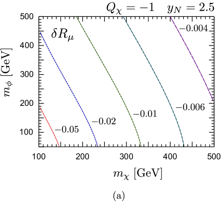
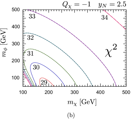
Figure 7: (a) Effect of vertex corrections on Rμsubscript𝑅𝜇R_{\mu}. δRμ=RμRμ𝛿subscript𝑅𝜇subscript𝑅𝜇superscriptsubscript𝑅𝜇\delta R_{\mu}=R_{\mu}-R_{\mu}^{\prime} are shown as a function of mχsubscript𝑚𝜒m_{\chi} and mϕsubscript𝑚italic-ϕm_{\phi} in case of Qχ=1subscript𝑄𝜒1Q_{\chi}=-1 and yN=2.5subscript𝑦𝑁2.5y_{N}=2.5, where Rμsubscript𝑅𝜇R_{\mu} includes all corrections, and Rμsuperscriptsubscript𝑅𝜇R_{\mu}^{\prime} contains all corrections except for the vertex corrections. (b) χ2superscript𝜒2\chi^{2} as a function of mχsubscript𝑚𝜒m_{\chi} and mϕsubscript𝑚italic-ϕm_{\phi} in case of Qχ=1subscript𝑄𝜒1Q_{\chi}=-1 and yN=2.5subscript𝑦𝑁2.5y_{N}=2.5.

Refer to caption Refer to caption

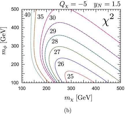
Figure 8: (a) Effect of vertex corrections on Rμsubscript𝑅𝜇R_{\mu}. δRμ=RμRμ𝛿subscript𝑅𝜇subscript𝑅𝜇superscriptsubscript𝑅𝜇\delta R_{\mu}=R_{\mu}-R_{\mu}^{\prime} is shown as a function of mχsubscript𝑚𝜒m_{\chi} and mϕsubscript𝑚italic-ϕm_{\phi} in case of Qχ=5subscript𝑄𝜒5Q_{\chi}=-5 and yN=1.5subscript𝑦𝑁1.5y_{N}=1.5, similar to Fig. 7(a). (b) χ2superscript𝜒2\chi^{2} as a function of mχsubscript𝑚𝜒m_{\chi} and mϕsubscript𝑚italic-ϕm_{\phi} in case of Qχ=5subscript𝑄𝜒5Q_{\chi}=-5 and yN=1.5subscript𝑦𝑁1.5y_{N}=1.5.

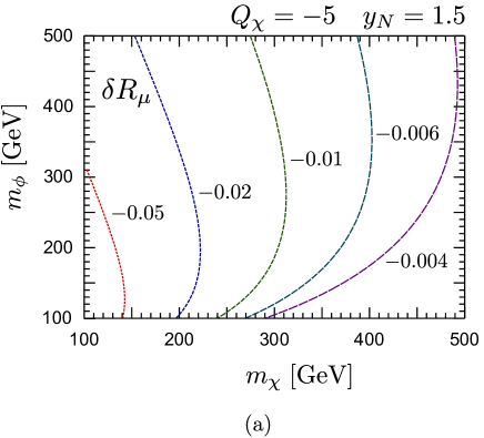
The vertex corrections affect EW observables such as Rμsubscript𝑅𝜇R_{\mu}, AFB0,μsubscriptsuperscript𝐴0𝜇FBA^{0,\mu}_{\rm FB}, and Aμsubscript𝐴𝜇A_{\mu}. Among these observables, we find that the effect on the Rμsubscript𝑅𝜇R_{\mu} is the most important in the fit because Rμsubscript𝑅𝜇R_{\mu} is most precisely measured. In Fig.7 (a), we show the effect of vertex corrections in Rμsubscript𝑅𝜇R_{\mu}, that is, δRμ=RμRμ𝛿subscript𝑅𝜇subscript𝑅𝜇superscriptsubscript𝑅𝜇\delta R_{\mu}=R_{\mu}-R_{\mu}^{\prime} as a function of mχsubscript𝑚𝜒m_{\chi} and mϕsubscript𝑚italic-ϕm_{\phi} in case of Qχ=1subscript𝑄𝜒1Q_{\chi}=-1 and yN=2.5subscript𝑦𝑁2.5y_{N}=2.5. Here Rμsubscript𝑅𝜇R_{\mu} is a theoretical prediction in this model containing all corrections, on the other hand, Rμsuperscriptsubscript𝑅𝜇R_{\mu}^{\prime} contains all corrections except for the vertex corrections. The difference δRμ𝛿subscript𝑅𝜇\delta R_{\mu} shows the effect of the vertex corrections. Note that the size of experimental error of Rμsubscript𝑅𝜇R_{\mu} is 0.0330.0330.033 for 1σ1𝜎1\sigma, as shown in Table. 1. As one can see in Fig. 7(a), the vertex correction can change the prediction of Rμsubscript𝑅𝜇R_{\mu} about 1σ1𝜎1\sigma in the region where the muon g-2 can be explained by the new physics contributions. Since the SM prediction of Rμsubscript𝑅𝜇R_{\mu} is smaller than that of the experimental result (shown in Table. 1), the vertex corrections do not help to improve the prediction of Rμsubscript𝑅𝜇R_{\mu}. Therefore, the region of small χ𝜒\chi mass is very constrained.

In Fig. 7 (b), χ2superscript𝜒2\chi^{2} is shown as a function of mχsubscript𝑚𝜒m_{\chi} and mϕsubscript𝑚italic-ϕm_{\phi} in case of Qχ=1subscript𝑄𝜒1Q_{\chi}=-1 and yN=2.5subscript𝑦𝑁2.5y_{N}=2.5. As one can see from the figure, χ2superscript𝜒2\chi^{2} is large in the region of small mχsubscript𝑚𝜒m_{\chi} because of the large vertex corrections, discussed above. In the region of larger mχsubscript𝑚𝜒m_{\chi} and mϕsubscript𝑚italic-ϕm_{\phi}, it is difficult to explain the anomaly of muon g-2 because new particles are too heavy, and hence the χ2superscript𝜒2\chi^{2} gets larger. The minimum of χ2superscript𝜒2\chi^{2} is around mχ200similar-tosubscript𝑚𝜒200m_{\chi}\sim 200 GeV and mϕ100similar-tosubscript𝑚italic-ϕ100m_{\phi}\sim 100 GeV, and we see that the light new particles are favored by the EW observables including muon g-2.

In Fig. 8 (a), the effect of vertex corrections on Rμsubscript𝑅𝜇R_{\mu}, δRμ𝛿subscript𝑅𝜇\delta R_{\mu} is shown in case of Qχ=5subscript𝑄𝜒5Q_{\chi}=-5 and yN=1.5subscript𝑦𝑁1.5y_{N}=1.5, similar to Fig. 7 (a). The vertex corrections can be as large as 1σ1𝜎1\sigma of the experimental error of Rμsubscript𝑅𝜇R_{\mu}, and they increase the χ2superscript𝜒2\chi^{2}. In Fig. 8 (b), the χ2superscript𝜒2\chi^{2} is shown as a function of mχsubscript𝑚𝜒m_{\chi} and mϕsubscript𝑚italic-ϕm_{\phi}. As one can see, the region of small mχsubscript𝑚𝜒m_{\chi} is disfavored by the vertex corrections of Rμsubscript𝑅𝜇R_{\mu}, as shown in Fig. 8 (a). The minimum of the χ2superscript𝜒2\chi^{2} is around mχ300similar-tosubscript𝑚𝜒300m_{\chi}\sim 300 GeV and mϕ100similar-tosubscript𝑚italic-ϕ100m_{\phi}\sim 100 GeV. Therefore, the EW precision measurements (including muon g-2) prefer the relatively light new particles in this case.

3.2 Model with SU(2) doublet (ΦΦ\Phi) and singlet (ϕitalic-ϕ\phi) scalar, and singlet fermion (χ𝜒\chi)

The singlet fermion contributions are same as those in the previous case. Here, we list the one loop contributions to gauge boson self-energies induced by scalar sectors.

ΠWW(s)(p2)superscriptsubscriptΠ𝑊𝑊𝑠superscript𝑝2\displaystyle\Pi_{WW}^{(s)}(p^{2}) =\displaystyle= g28π2[i{|V2i|2B22(ϕ1,si)14|V2i|2A(si)}14A(ϕ1)],superscript𝑔28superscript𝜋2delimited-[]subscript𝑖superscriptsubscript𝑉2𝑖2subscript𝐵22subscriptitalic-ϕ1subscript𝑠𝑖14superscriptsubscript𝑉2𝑖2𝐴subscript𝑠𝑖14𝐴subscriptitalic-ϕ1\displaystyle\frac{g^{2}}{8\pi^{2}}\left[\sum_{i}\left\{|V_{2i}|^{2}B_{22}(\phi_{1},s_{i})-\frac{1}{4}|V_{2i}|^{2}A({s_{i}})\right\}-\frac{1}{4}A(\phi_{1})\right], (3.41)
ΠZZ(s)(p2)superscriptsubscriptΠ𝑍𝑍𝑠superscript𝑝2\displaystyle\Pi_{ZZ}^{(s)}(p^{2}) =\displaystyle= 14πg2cW2[(12Q1sW2)2{B22(ϕ1,ϕ1)12A(ϕ1)}\displaystyle\frac{1}{4\pi}\frac{g^{2}}{c_{W}^{2}}\left[\left(\frac{1}{2}-Q_{1}s_{W}^{2}\right)^{2}\left\{B_{22}(\phi_{1},\phi_{1})-\frac{1}{2}A(\phi_{1})\right\}\right. (3.42)
+ij{(12Q2sW2)2|V2i|2|V2j|2+Q22sW4|V1i|2|V1j|2\displaystyle+\sum_{ij}\left\{\left(-\frac{1}{2}-Q_{2}s_{W}^{2}\right)^{2}|V_{2i}|^{2}|V_{2j}|^{2}+Q_{2}^{2}s_{W}^{4}|V_{1i}|^{2}|V_{1j}|^{2}\right.
Q2sW2(12Q2sW2)(V2iV1iV1jV2j+V2jV1jV1iV2i)}B22(si,sj)\displaystyle-\left.Q_{2}s_{W}^{2}\left(-\frac{1}{2}-Q_{2}s_{W}^{2}\right)(V_{2i}^{*}V_{1i}V_{1j}^{*}V_{2j}+V_{2j}^{*}V_{1j}V_{1i}^{*}V_{2i})\right\}B_{22}(s_{i},s_{j})
i{(12Q2sW2)2|V2i|2+Q22sW4|V1i|2}12A(si)],\displaystyle\left.-\sum_{i}\left\{\left(-\frac{1}{2}-Q_{2}s_{W}^{2}\right)^{2}|V_{2i}|^{2}+Q_{2}^{2}s_{W}^{4}|V_{1i}|^{2}\right\}\frac{1}{2}A(s_{i})\right],
Πγγ(s)(p2)superscriptsubscriptΠ𝛾𝛾𝑠superscript𝑝2\displaystyle\Pi_{\gamma\gamma}^{(s)}(p^{2}) =\displaystyle= e24π2[Q12{B22(ϕ1,ϕ1)12A(ϕ1)}\displaystyle\frac{e^{2}}{4\pi^{2}}\left[Q_{1}^{2}\left\{B_{22}(\phi_{1},\phi_{1})-\frac{1}{2}A(\phi_{1})\right\}\right. (3.43)
+Q22i{B22(si,si)12A(si)}],\displaystyle~{}~{}~{}~{}~{}~{}~{}~{}~{}~{}~{}~{}~{}~{}~{}~{}~{}~{}~{}~{}~{}~{}~{}~{}~{}+\left.Q_{2}^{2}\sum_{i}\left\{B_{22}(s_{i},s_{i})-\frac{1}{2}A(s_{i})\right\}\right],
ΠγZ(s)(p2)superscriptsubscriptΠ𝛾𝑍𝑠superscript𝑝2\displaystyle\Pi_{\gamma Z}^{(s)}(p^{2}) =\displaystyle= e4π2gcW[Q1(12Q1sW2){B22(ϕ1,ϕ1)12A(ϕ1)}\displaystyle\frac{e}{4\pi^{2}}\frac{g}{c_{W}}\left[Q_{1}\left(\frac{1}{2}-Q_{1}s_{W}^{2}\right)\left\{B_{22}(\phi_{1},\phi_{1})-\frac{1}{2}A(\phi_{1})\right\}\right. (3.44)
+Q2i{(12Q2sW2)|V2i|2Q2sW2|V1i|2}subscript𝑄2subscript𝑖12subscript𝑄2superscriptsubscript𝑠𝑊2superscriptsubscript𝑉2𝑖2subscript𝑄2superscriptsubscript𝑠𝑊2superscriptsubscript𝑉1𝑖2\displaystyle+Q_{2}\sum_{i}\left\{\left(-\frac{1}{2}-Q_{2}s_{W}^{2}\right)|V_{2i}|^{2}-Q_{2}s_{W}^{2}|V_{1i}|^{2}\right\}
×{B22(si,si)12A(si)}],\displaystyle\left.~{}~{}~{}~{}~{}~{}~{}~{}~{}~{}~{}~{}~{}~{}~{}~{}~{}~{}~{}~{}~{}~{}~{}~{}~{}~{}\times\left\{B_{22}(s_{i},s_{i})-\frac{1}{2}A(s_{i})\right\}\right],

where Passarino-Veltman functions BX(i,j)(=BX(mi2,mj2;p))annotatedsubscript𝐵𝑋𝑖𝑗absentsubscript𝐵𝑋superscriptsubscript𝑚𝑖2superscriptsubscript𝑚𝑗2𝑝B_{X}(i,j)(=B_{X}(m_{i}^{2},m_{j}^{2};p)) and A(i)𝐴𝑖A(i) are shown in Appendix. Unlike the previous model, SU(2) scalar doublet can contribute to the STU parameters. Therefore, the dominant quantum corrections are represented by S and T parameters. To understand a behavior of S and T parameters, here we show the approximate expression of S and T parameters,

S𝑆\displaystyle S similar-to-or-equals\displaystyle\simeq YΦ6πΔ+,subscript𝑌Φ6𝜋Δ\displaystyle\frac{Y_{\Phi}}{6\pi}\Delta+\cdots,
T𝑇\displaystyle T similar-to-or-equals\displaystyle\simeq mϕ1216πsW2MW2(Δ)2+.superscriptsubscript𝑚subscriptitalic-ϕ1216𝜋superscriptsubscript𝑠𝑊2superscriptsubscript𝑀𝑊2superscriptΔ2\displaystyle\frac{m_{\phi_{1}}^{2}}{16\pi s_{W}^{2}M_{W}^{2}}(\Delta)^{2}+\cdots. (3.45)

Here, for simplicity, we assume that V22=V11=1,V12=V21=0formulae-sequencesubscript𝑉22subscript𝑉111subscript𝑉12subscript𝑉210V_{22}=V_{11}=1,~{}V_{12}=V_{21}=0 so that s2subscript𝑠2s_{2} state originates from ϕ2subscriptitalic-ϕ2\phi_{2} component of SU(2) scalar doublet ΦΦ\Phi, and Δ=(mϕ22mϕ12)/mϕ12Δsuperscriptsubscript𝑚subscriptitalic-ϕ22superscriptsubscript𝑚subscriptitalic-ϕ12superscriptsubscript𝑚subscriptitalic-ϕ12\Delta=(m_{\phi_{2}}^{2}-m_{\phi_{1}}^{2})/m_{\phi_{1}}^{2} where mϕ2=ms2subscript𝑚subscriptitalic-ϕ2subscript𝑚subscript𝑠2m_{\phi_{2}}=m_{s_{2}} in this case. Here we ignore the higher order terms of ΔΔ\Delta and mZ2/mϕ12superscriptsubscript𝑚𝑍2superscriptsubscript𝑚subscriptitalic-ϕ12m_{Z}^{2}/m_{\phi_{1}}^{2} in Eqs. (3.45). Note that ΔΔ\Delta parameterizes non-degeneracy in the SU(2) scalar doublet ΦΦ\Phi. YΦsubscript𝑌ΦY_{\Phi} is a hypercharge of ΦΦ\Phi, YΦ=12+Q2subscript𝑌Φ12subscript𝑄2Y_{\Phi}=\frac{1}{2}+Q_{2}. We note that the non-degeneracy of SU(2) scalar doublet generates non-zero T and non-zero S, and T is always positive, but S can be positive or negative depending on signs of YΦsubscript𝑌ΦY_{\Phi} and ΔΔ\Delta in this model.

Refer to caption

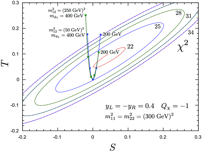
Figure 9: χ2superscript𝜒2\chi^{2} contours (without including muon g-2 result) in S-T plane ( χ2=22superscript𝜒222\chi^{2}=22 to 34 in dashed lines) and S-T values (solid lines with points) in this model. Here we take yL=yR=0.4subscript𝑦𝐿subscript𝑦𝑅0.4y_{L}=-y_{R}=0.4, Qχ=1subscript𝑄𝜒1Q_{\chi}=-1 (corresponding to Q1=1subscript𝑄11Q_{1}=1 and Q2=0subscript𝑄20Q_{2}=0), and m112=m222=(300GeV)2superscriptsubscript𝑚112superscriptsubscript𝑚222superscript300GeV2m_{11}^{2}=m_{22}^{2}=(300~{}{\rm GeV})^{2}. Two solid lines correspond to two different values of m122superscriptsubscript𝑚122m_{12}^{2}, m122=(50GeV)2superscriptsubscript𝑚122superscript50GeV2m_{12}^{2}=(50~{}{\rm GeV})^{2} and (250GeV)2superscript250GeV2(250~{}{\rm GeV})^{2}, varying mϕ1subscript𝑚subscriptitalic-ϕ1m_{\phi_{1}} from 200 GeV to 400 GeV at 50 GeV step.

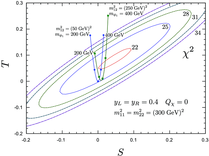
In Fig. 9, we show numerical result of χ2superscript𝜒2\chi^{2} contours in S-T plane (without including muon g-2 result), shown in dashed lines. To draw the χ2superscript𝜒2\chi^{2} contours in S-T plane, we assume that other oblique corrections (U𝑈U, RZsubscript𝑅𝑍R_{Z}, and RWsubscript𝑅𝑊R_{W}) and vertex corrections are zero. As one can see from the figure, slightly positive S and T (S0.05similar-to𝑆0.05S\sim 0.05 and T0.1similar-to𝑇0.1T\sim 0.1) are favored by EW observables. In Fig. 9, we also show the predicted values of S-T parameters in this model, shown in solid lines. Here we took yL=yR=0.4subscript𝑦𝐿subscript𝑦𝑅0.4y_{L}=-y_{R}=0.4, Qχ=1subscript𝑄𝜒1Q_{\chi}=-1 (corresponding to Q1=1subscript𝑄11Q_{1}=1 and Q2=0subscript𝑄20Q_{2}=0), and m112=m222=(300GeV)2superscriptsubscript𝑚112superscriptsubscript𝑚222superscript300GeV2m_{11}^{2}=m_{22}^{2}=(300~{}{\rm GeV})^{2}. Two solid lines correspond to two different values of m122superscriptsubscript𝑚122m_{12}^{2}, m122=(50GeV)2superscriptsubscript𝑚122superscript50GeV2m_{12}^{2}=(50~{}{\rm GeV})^{2} and (250GeV)2superscript250GeV2(250~{}{\rm GeV})^{2}. The points on the solid lines represent the predicted values of S and T, varying mϕ1subscript𝑚subscriptitalic-ϕ1m_{\phi_{1}} from 200 GeV to 400 GeV at 50 GeV step.

When m112=m222=(300GeV)2superscriptsubscript𝑚112superscriptsubscript𝑚222superscript300GeV2m_{11}^{2}=m_{22}^{2}=(300~{}{\rm GeV})^{2} and m122=(50GeV)2superscriptsubscript𝑚122superscript50GeV2m_{12}^{2}=(50~{}{\rm GeV})^{2}, ms1296similar-to-or-equalssubscript𝑚subscript𝑠1296m_{s_{1}}\simeq 296 GeV and ms2304similar-to-or-equalssubscript𝑚subscript𝑠2304m_{s_{2}}\simeq 304 GeV. As roughly shown in Eqs. (3.45), when mϕ1=200subscript𝑚subscriptitalic-ϕ1200m_{\phi_{1}}=200 GeV and Q2=0subscript𝑄20Q_{2}=0, Δ>0Δ0\Delta>0 and YΦ=12>0subscript𝑌Φ120Y_{\Phi}=\frac{1}{2}>0, and hence S>0𝑆0S>0 and T>0𝑇0T>0. As mϕ1subscript𝑚subscriptitalic-ϕ1m_{\phi_{1}} becomes larger and about 300 GeV, both S𝑆S and T𝑇T get closer to zero because the doublet scalars are almost degenerate. Then when mϕ1subscript𝑚subscriptitalic-ϕ1m_{\phi_{1}} is increased further, S𝑆S gets negative because Δ<0Δ0\Delta<0, but T>0𝑇0T>0. In Fig. 9, one can see this behavior. Even when we increase m122superscriptsubscript𝑚122m_{12}^{2}, we can see that this behavior is almost same.
Refer to caption

Figure 10: Same as Fig. 9 except for yL=yR=0.4subscript𝑦𝐿subscript𝑦𝑅0.4y_{L}=y_{R}=0.4 and Qχ=0subscript𝑄𝜒0Q_{\chi}=0 (corresponding to Q1=0subscript𝑄10Q_{1}=0 and Q2=1subscript𝑄21Q_{2}=-1).

In Fig. 10, the same figure is shown except for yL=yR=0.4subscript𝑦𝐿subscript𝑦𝑅0.4y_{L}=y_{R}=0.4 and Qχ=0subscript𝑄𝜒0Q_{\chi}=0 (corresponding to Q1=0subscript𝑄10Q_{1}=0 and Q2=1subscript𝑄21Q_{2}=-1). When Qχ=0subscript𝑄𝜒0Q_{\chi}=0 (Q2=1subscript𝑄21Q_{2}=-1) and mϕ1=200subscript𝑚subscriptitalic-ϕ1200m_{\phi_{1}}=200 GeV, YΦ=12<0subscript𝑌Φ120Y_{\Phi}=-\frac{1}{2}<0 and Δ>0Δ0\Delta>0, so that S𝑆S is negative. As mϕ1subscript𝑚subscriptitalic-ϕ1m_{\phi_{1}} gets larger, S𝑆S gets larger. For mϕ1300similar-tosubscript𝑚subscriptitalic-ϕ1300m_{\phi_{1}}\sim 300 GeV, S0similar-to𝑆0S\sim 0 because the doublet scalars are almost degenerate. For mϕ1>300subscript𝑚subscriptitalic-ϕ1300m_{\phi_{1}}>300 GeV, S𝑆S becomes positive. This behavior is different from the previous case with Q2=0subscript𝑄20Q_{2}=0 since the sign of YΦsubscript𝑌ΦY_{\Phi} is different. Note that T𝑇T is always positive unless SU(2) scalar doublet is degenerate. As one can see in both cases, the small non-degeneracy of SU(2) scalar doublet can make χ2superscript𝜒2\chi^{2} better.

In our numerical analysis, we also include the vertex corrections in Zμ+μ𝑍superscript𝜇superscript𝜇Z\mu^{+}\mu^{-}, Zνμν¯μ𝑍subscript𝜈𝜇subscript¯𝜈𝜇Z\nu_{\mu}\bar{\nu}_{\mu} and Wμνμ𝑊𝜇subscript𝜈𝜇W\mu\nu_{\mu} vertices even though the Yukawa couplings yLsubscript𝑦𝐿y_{L} and yRsubscript𝑦𝑅y_{R} can be small in this model. The expression of the vertex corrections is summarized as follows:

ΔgLμΔsuperscriptsubscript𝑔𝐿𝜇\displaystyle\Delta g_{L}^{\mu} =\displaystyle= yL216π2[2ij{(12QϕsW2)V2iV2jQϕsW2V1iV1j}V2iV2jC24(si,χ,sj;p,qp)\displaystyle\frac{y_{L}^{2}}{16\pi^{2}}\left[2\sum_{ij}\left\{\left(-\frac{1}{2}-Q_{\phi}s_{W}^{2}\right)V_{2i}^{*}V_{2j}-Q_{\phi}s_{W}^{2}V_{1i}^{*}V_{1j}\right\}V_{2i}V_{2j}^{*}C_{24}(s_{i},\chi,s_{j};p,q-p)\right. (3.46)
+iQχsW2|V2i|2{122C24MZ2(C12+C23)+mχ2C0}(χ,si,χ;qp,p)subscript𝑖subscript𝑄𝜒superscriptsubscript𝑠𝑊2superscriptsubscript𝑉2𝑖2122subscript𝐶24superscriptsubscript𝑀𝑍2subscript𝐶12subscript𝐶23superscriptsubscript𝑚𝜒2subscript𝐶0𝜒subscript𝑠𝑖𝜒𝑞𝑝𝑝\displaystyle+\sum_{i}Q_{\chi}s_{W}^{2}|V_{2i}|^{2}\left\{\frac{1}{2}-2C_{24}-M_{Z}^{2}(C_{12}+C_{23})+m_{\chi}^{2}C_{0}\right\}(\chi,s_{i},\chi;q-p,p)
i(12+sW2)|V2i|2(B0+B1)(si,χ;p)],\displaystyle\left.-\sum_{i}\left(-\frac{1}{2}+s_{W}^{2}\right)|V_{2i}|^{2}(B_{0}+B_{1})(s_{i},\chi;p)\right],
ΔgRμΔsuperscriptsubscript𝑔𝑅𝜇\displaystyle\Delta g_{R}^{\mu} =\displaystyle= yR216π2[2ij{(12QϕsW2)V2iV2jQϕsW2V1iV1j}V1iV1jC24(si,χ,sj;p,qp)\displaystyle\frac{y_{R}^{2}}{16\pi^{2}}\left[2\sum_{ij}\left\{\left(-\frac{1}{2}-Q_{\phi}s_{W}^{2}\right)V_{2i}^{*}V_{2j}-Q_{\phi}s_{W}^{2}V_{1i}^{*}V_{1j}\right\}V_{1i}V_{1j}^{*}C_{24}(s_{i},\chi,s_{j};p,q-p)\right. (3.47)
+iQχsW2|V1i|2{122C24MZ2(C12+C23)+mχ2C0}(χ,si,χ;qp,p)subscript𝑖subscript𝑄𝜒superscriptsubscript𝑠𝑊2superscriptsubscript𝑉1𝑖2122subscript𝐶24superscriptsubscript𝑀𝑍2subscript𝐶12subscript𝐶23superscriptsubscript𝑚𝜒2subscript𝐶0𝜒subscript𝑠𝑖𝜒𝑞𝑝𝑝\displaystyle+\sum_{i}Q_{\chi}s_{W}^{2}|V_{1i}|^{2}\left\{\frac{1}{2}-2C_{24}-M_{Z}^{2}(C_{12}+C_{23})+m_{\chi}^{2}C_{0}\right\}(\chi,s_{i},\chi;q-p,p)
isW2|V1i|2(B0+B1)(si,χ;p)],\displaystyle\left.-\sum_{i}s_{W}^{2}|V_{1i}|^{2}(B_{0}+B_{1})(s_{i},\chi;p)\right],
ΔgLνμΔsuperscriptsubscript𝑔𝐿subscript𝜈𝜇\displaystyle\Delta g_{L}^{\nu_{\mu}} =\displaystyle= yN216π2[2(12sW2Qϕ1)C24(ϕ1,χ,ϕ1;qp,p)\displaystyle\frac{y_{N}^{2}}{16\pi^{2}}\left[2\left(\frac{1}{2}-s_{W}^{2}Q_{\phi_{1}}\right)C_{24}(\phi_{1},\chi,\phi_{1};q-p,p)\right. (3.48)
+QχsW2{122C24MZ2(C12+C23)+mχ2C0}(χ,ϕ1,χ;qp,p)subscript𝑄𝜒superscriptsubscript𝑠𝑊2122subscript𝐶24superscriptsubscript𝑀𝑍2subscript𝐶12subscript𝐶23superscriptsubscript𝑚𝜒2subscript𝐶0𝜒subscriptitalic-ϕ1𝜒𝑞𝑝𝑝\displaystyle+Q_{\chi}s_{W}^{2}\left\{\frac{1}{2}-2C_{24}-M_{Z}^{2}(C_{12}+C_{23})+m_{\chi}^{2}C_{0}\right\}(\chi,\phi_{1},\chi;q-p,p)
12(B0+B1)(ϕ1,χ;p)],\displaystyle\left.-\frac{1}{2}(B_{0}+B_{1})(\phi_{1},\chi;p)\right],

where p𝑝p and q𝑞q are momenta for muon in ΔgL,RμΔsubscriptsuperscript𝑔𝜇𝐿𝑅\Delta g^{\mu}_{L,R}(muon neutrino in ΔgLνμΔsubscriptsuperscript𝑔subscript𝜈𝜇𝐿\Delta g^{\nu_{\mu}}_{L}) and Z-boson, respectively. Correction to μνμW𝜇subscript𝜈𝜇𝑊\mu\nu_{\mu}W-vertex is written by

Δδ¯GΔsubscript¯𝛿𝐺\displaystyle\Delta\bar{\delta}_{G} =\displaystyle= yL28π2[i|V2i|2C24(ϕ1,si,χ;q,p)\displaystyle\frac{y_{L}^{2}}{8\pi^{2}}\left[\sum_{i}|V_{2i}|^{2}C_{24}(\phi_{1},s_{i},\chi;-q,p)\right. (3.49)
14{(B0+B1)(ϕ1,χ;pq)+i|V2i|2(B0+B1)(si,χ;p)}],\displaystyle\left.-\frac{1}{4}\left\{(B_{0}+B_{1})(\phi_{1},\chi;p-q)+\sum_{i}|V_{2i}|^{2}(B_{0}+B_{1})(s_{i},\chi;p)\right\}\right],

where p𝑝p, pq𝑝𝑞p-q and q𝑞q are momenta for muon, muon-neutrino, and W-boson, respectively. Here we use approximation q2=0superscript𝑞20q^{2}=0.

Refer to caption Refer to caption

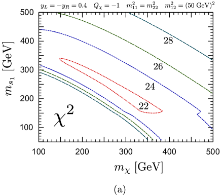
Figure 11: χ2superscript𝜒2\chi^{2} contours as a function of mχsubscript𝑚𝜒m_{\chi} and ms1subscript𝑚subscript𝑠1m_{s_{1}} in case of (a) Qχ=1subscript𝑄𝜒1Q_{\chi}=-1 and yL=yR=0.4subscript𝑦𝐿subscript𝑦𝑅0.4y_{L}=-y_{R}=0.4 and (b) Qχ=0subscript𝑄𝜒0Q_{\chi}=0 and yL=yR=0.4subscript𝑦𝐿subscript𝑦𝑅0.4y_{L}=y_{R}=0.4. Here we take m112=m222superscriptsubscript𝑚112superscriptsubscript𝑚222m_{11}^{2}=m_{22}^{2} and m122=(50GeV)2superscriptsubscript𝑚122superscript50GeV2m_{12}^{2}=(50~{}{\rm GeV})^{2}.

In Fig. 11, we show χ2superscript𝜒2\chi^{2} contours as a function of mχsubscript𝑚𝜒m_{\chi} and ms1subscript𝑚subscript𝑠1m_{s_{1}} in case of (a) Qχ=1subscript𝑄𝜒1Q_{\chi}=-1 and yL=yR=0.4subscript𝑦𝐿subscript𝑦𝑅0.4y_{L}=-y_{R}=0.4 and (b) Qχ=0subscript𝑄𝜒0Q_{\chi}=0 and yL=yR=0.4subscript𝑦𝐿subscript𝑦𝑅0.4y_{L}=y_{R}=0.4. Here we have taken m122=(50GeV)2superscriptsubscript𝑚122superscript50GeV2m_{12}^{2}=(50~{}{\rm GeV})^{2}, and m112=m222superscriptsubscript𝑚112superscriptsubscript𝑚222m_{11}^{2}=m_{22}^{2}. mϕ1subscript𝑚subscriptitalic-ϕ1m_{\phi_{1}} is chosen so that the χ2superscript𝜒2\chi^{2} becomes the smallest, provided that mϕ1>105GeVsubscript𝑚subscriptitalic-ϕ1105GeVm_{\phi_{1}}>105~{}{\rm GeV} for Qχ=1subscript𝑄𝜒1Q_{\chi}=-1 and mϕ1>46GeVsubscript𝑚subscriptitalic-ϕ146GeVm_{\phi_{1}}>46~{}{\rm GeV} for Qχ=0subscript𝑄𝜒0Q_{\chi}=0 respectively. In both cases shown in Fig. 11, the χ2superscript𝜒2\chi^{2} can be as small as 22, which is smaller than those in the previous case where only right-handed muon has new Yukawa coupling. As seen from Fig. 11, the relatively light χ𝜒\chi and sisubscript𝑠𝑖s_{i} are favored by the EW observables. In Table. 1, we show the predicted values of the EW observables in case of Qχ=0subscript𝑄𝜒0Q_{\chi}=0, mϕ1=300subscript𝑚subscriptitalic-ϕ1300m_{\phi_{1}}=300 GeV, mχ=200subscript𝑚𝜒200m_{\chi}=200 GeV, m112=m222=(250)2superscriptsubscript𝑚112superscriptsubscript𝑚222superscript2502m_{11}^{2}=m_{22}^{2}=(250)^{2} GeV2, and m122=(50)2superscriptsubscript𝑚122superscript502m_{12}^{2}=(50)^{2} GeV2. As shown in Table. 1, the fit is quite good. Therefore, it will be important to know what kind of effects we expect from these particles at the LHC. In a next section, we will discuss the possible effects of these new particles at the LHC.

4 Phenomenology at the LHC

In the previous section, we show that in order to explain the anomaly of muon g-2, it is strongly suggested that there should be the EW scale new particles. It is also suggested that multi-charged particles may be favored by the anomaly of muon g-2. Therefore, these particles may be reachable directly and/or indirectly at the LHC. Here we discuss the effects of these new particles in the Higgs decay hγγ𝛾𝛾h\rightarrow\gamma\gamma and their direct productions at the LHC.

4.1 hγγ𝛾𝛾h\rightarrow\gamma\gamma

The SU(2) singlet and doublet scalars can couple to the Higgs boson through the following scalar interactions:

\displaystyle\cal{L} =\displaystyle= κ1ϕϕ(HH)κ2(ΦΦ)(HH)κ3(HΦ)(ΦH)subscript𝜅1superscriptitalic-ϕitalic-ϕsuperscript𝐻𝐻subscript𝜅2superscriptΦΦsuperscript𝐻𝐻subscript𝜅3superscript𝐻ΦsuperscriptΦ𝐻\displaystyle-\kappa_{1}\phi^{\dagger}\phi(H^{\dagger}H)-\kappa_{2}(\Phi^{\dagger}\Phi)(H^{\dagger}H)-\kappa_{3}(H^{\dagger}\Phi)(\Phi^{\dagger}H) (4.50)
κ4M{(HΦ)ϕ+h.c.},\displaystyle-\kappa_{4}M\left\{(H^{\dagger}\Phi)\phi^{\dagger}~{}{\rm+h.c.}\right\},

where H𝐻H is a standard model Higgs boson doublet. In case where only SU(2) singlet scalar ϕitalic-ϕ\phi exists, only coupling κ1subscript𝜅1\kappa_{1} is non-zero, but in case where both SU(2) singlet ϕitalic-ϕ\phi and doublet ΦΦ\Phi scalars are there, all couplings are allowed#6#6#6 When the QED charge of ϕitalic-ϕ\phi (Qϕsubscript𝑄italic-ϕQ_{\phi}) is zero, terms such as (HΦ)ϕsuperscript𝐻Φitalic-ϕ(H^{\dagger}\Phi)\phi and (HΦ)2superscriptsuperscript𝐻Φ2(H^{\dagger}\Phi)^{2} are also possible. In our analysis, we assume that such terms are small, for simplicity. Even if we include such terms, our result does not change qualitatively. .

In the case where only right-handed muon has new Yukawa interaction, there is SU(2) singlet ϕitalic-ϕ\phi, and its interaction with Higgs boson is

=λvhϕϕ,𝜆𝑣superscriptitalic-ϕitalic-ϕ\displaystyle{\cal{L}}=-\lambda vh\phi^{\dagger}\phi, (4.51)

where λ=κ1𝜆subscript𝜅1\lambda=\kappa_{1} in this model and v𝑣v is a vacuum expectation value of Higgs field, v246similar-to-or-equals𝑣246v\simeq 246 GeV. When Qϕsubscript𝑄italic-ϕQ_{\phi}, which is the QED charge of ϕitalic-ϕ\phi, is non-zero, ϕitalic-ϕ\phi can contribute to the Higgs decay hγγ𝛾𝛾h\rightarrow\gamma\gamma. The decay width Γ(hγγ)Γ𝛾𝛾\Gamma(h\rightarrow\gamma\gamma) is given by

Γ(hγγ)Γ𝛾𝛾\displaystyle\Gamma(h\rightarrow\gamma\gamma) =\displaystyle= α2mh3256π3v2|S(mh)|2,superscript𝛼2superscriptsubscript𝑚3256superscript𝜋3superscript𝑣2superscript𝑆subscript𝑚2\displaystyle\frac{\alpha^{2}m_{h}^{3}}{256\pi^{3}v^{2}}|S(m_{h})|^{2}, (4.52)

where the amplitude S(mh)𝑆subscript𝑚S(m_{h}) at leading order is written by

S(mh)=83Ft(τt)FW(τW)+Qϕ2λv22mϕ2Fϕ(τϕ).𝑆subscript𝑚83subscript𝐹𝑡subscript𝜏𝑡subscript𝐹𝑊subscript𝜏𝑊superscriptsubscript𝑄italic-ϕ2𝜆superscript𝑣22superscriptsubscript𝑚italic-ϕ2subscript𝐹italic-ϕsubscript𝜏italic-ϕ\displaystyle S(m_{h})=\frac{8}{3}F_{t}(\tau_{t})-F_{W}(\tau_{W})+Q_{\phi}^{2}\lambda\frac{v^{2}}{2m_{\phi}^{2}}F_{\phi}(\tau_{\phi}). (4.53)

Here the first, the second, and the third terms are top, W, and ϕitalic-ϕ\phi contributions, respectively, and τx=mh24mx2(x=t,W,ϕ)subscript𝜏𝑥superscriptsubscript𝑚24superscriptsubscript𝑚𝑥2𝑥𝑡𝑊italic-ϕ\tau_{x}=\frac{m_{h}^{2}}{4m_{x}^{2}}~{}(x=t,W,~{}\phi). The function Ft,FW,Fϕsubscript𝐹𝑡subscript𝐹𝑊subscript𝐹italic-ϕF_{t},~{}F_{W},~{}F_{\phi} are given by

Ft(τ)subscript𝐹𝑡𝜏\displaystyle F_{t}(\tau) =\displaystyle= τ1[1+(1τ1)f(τ)],superscript𝜏1delimited-[]11superscript𝜏1𝑓𝜏\displaystyle\tau^{-1}\left[1+(1-\tau^{-1})f(\tau)\right], (4.54)
FW(τ)subscript𝐹𝑊𝜏\displaystyle F_{W}(\tau) =\displaystyle= 2+3τ1+3τ1(2τ1)f(τ),23superscript𝜏13superscript𝜏12superscript𝜏1𝑓𝜏\displaystyle 2+3\tau^{-1}+3\tau^{-1}(2-\tau^{-1})f(\tau), (4.55)
Fϕ(τϕ)subscript𝐹italic-ϕsubscript𝜏italic-ϕ\displaystyle F_{\phi}(\tau_{\phi}) =\displaystyle= τ1[1+τ1f(τ)],superscript𝜏1delimited-[]1superscript𝜏1𝑓𝜏\displaystyle\tau^{-1}\left[-1+\tau^{-1}f(\tau)\right], (4.56)

where f(τ)=arcsin2(τ)𝑓𝜏superscript2𝜏f(\tau)=\arcsin^{2}(\sqrt{\tau}) for τ<1𝜏1\tau<1. Branching ratio of hγγ𝛾𝛾h\rightarrow\gamma\gamma is approximately given by

BR(hγγ)BR(hγγ)SMBR𝛾𝛾BRsubscript𝛾𝛾SM\displaystyle\frac{{\rm BR}(h\rightarrow\gamma\gamma)}{{\rm BR}(h\rightarrow\gamma\gamma)_{\rm SM}} similar-to-or-equals\displaystyle\simeq Γ(hγγ)Γ(hγγ)SM=|83Ft(τt)FW(τW)+Qϕ2λv22mϕ2Fϕ(τϕ)83Ft(τt)FW(τW)|2,Γ𝛾𝛾Γsubscript𝛾𝛾SMsuperscript83subscript𝐹𝑡subscript𝜏𝑡subscript𝐹𝑊subscript𝜏𝑊superscriptsubscript𝑄italic-ϕ2𝜆superscript𝑣22superscriptsubscript𝑚italic-ϕ2subscript𝐹italic-ϕsubscript𝜏italic-ϕ83subscript𝐹𝑡subscript𝜏𝑡subscript𝐹𝑊subscript𝜏𝑊2\displaystyle\frac{\Gamma(h\rightarrow\gamma\gamma)}{\Gamma(h\rightarrow\gamma\gamma)_{\rm SM}}=\left|\frac{\frac{8}{3}F_{t}(\tau_{t})-F_{W}(\tau_{W})+Q_{\phi}^{2}\lambda\frac{v^{2}}{2m_{\phi}^{2}}F_{\phi}(\tau_{\phi})}{\frac{8}{3}F_{t}(\tau_{t})-F_{W}(\tau_{W})}\right|^{2}, (4.57)

because the total decay width does not change much, even if Γ(hγγ)Γ𝛾𝛾\Gamma(h\rightarrow\gamma\gamma) changes. Here BR(hγγ)SMBRsubscript𝛾𝛾SM{\rm BR}(h\rightarrow\gamma\gamma)_{\rm SM} and Γ(hγγ)SMΓsubscript𝛾𝛾SM\Gamma(h\rightarrow\gamma\gamma)_{\rm SM} are the SM predictions at the leading order.
Refer to caption

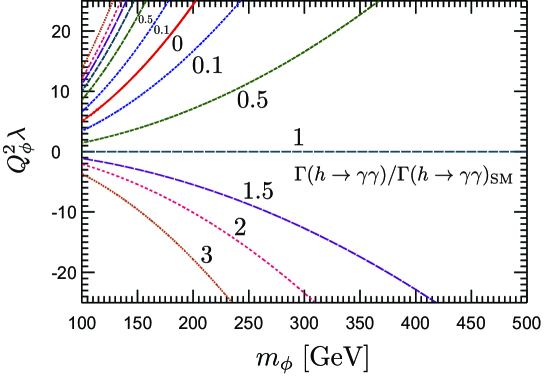
Figure 12: Higgs decay width hγγ𝛾𝛾h\rightarrow\gamma\gamma normalized by the SM prediction Γ(hγγ)Γ(hγγ)SMΓ𝛾𝛾Γsubscript𝛾𝛾SM\frac{\Gamma(h\rightarrow\gamma\gamma)}{\Gamma(h\rightarrow\gamma\gamma)_{\rm SM}} as a function of mϕsubscript𝑚italic-ϕm_{\phi} and Qϕ2λsuperscriptsubscript𝑄italic-ϕ2𝜆Q_{\phi}^{2}\lambda. Here we take mh=125subscript𝑚125m_{h}=125 GeV.

Notice that this ratio is a function of mϕsubscript𝑚italic-ϕm_{\phi} and Qϕ2λsuperscriptsubscript𝑄italic-ϕ2𝜆Q_{\phi}^{2}\lambda when Higgs boson mass mhsubscript𝑚m_{h} is fixed. As we discussed earlier, in order to explain the anomaly of muon g-2, larger Qϕsubscript𝑄italic-ϕQ_{\phi} may be favored. As can be seen in Eq. (4.57), larger Qϕsubscript𝑄italic-ϕQ_{\phi} induces larger effect on hγγ𝛾𝛾h\rightarrow\gamma\gamma.

In Fig. 12, the ratio Γ(hγγ)/Γ(hγγ)SMΓ𝛾𝛾Γsubscript𝛾𝛾SM{\Gamma(h\rightarrow\gamma\gamma)}/{\Gamma(h\rightarrow\gamma\gamma)_{\rm SM}} is shown as a function of mϕsubscript𝑚italic-ϕm_{\phi} and Qϕ2λsuperscriptsubscript𝑄italic-ϕ2𝜆Q_{\phi}^{2}\lambda. Here we took mh=125subscript𝑚125m_{h}=125 GeV. As one can see from the figure, the effect can be significant if Qϕ2λsuperscriptsubscript𝑄italic-ϕ2𝜆Q_{\phi}^{2}\lambda is large and mϕsubscript𝑚italic-ϕm_{\phi} is O(100)𝑂100O(100) GeV. For example, as we discussed, when Qϕ=4subscript𝑄italic-ϕ4Q_{\phi}=4, λ=1(1)𝜆11\lambda=1~{}(-1) and mϕ=200subscript𝑚italic-ϕ200m_{\phi}=200 GeV, Γ(hγγ)/Γ(hγγ)SM=0.12(2.7)Γ𝛾𝛾Γsubscript𝛾𝛾SM0.122.7{\Gamma(h\rightarrow\gamma\gamma)}/{\Gamma(h\rightarrow\gamma\gamma)_{\rm SM}}=0.12~{}(2.7). Unfortunately, we can not predict the branching ratio BR(hγγ)BR𝛾𝛾{\rm BR}(h\rightarrow\gamma\gamma) in this model because λ𝜆\lambda is unknown. However, it is not surprising that BR(hγγ)BR𝛾𝛾{\rm BR}(h\rightarrow\gamma\gamma) is very different from the SM prediction.

In the case where both right- and left-handed muons have new Yukawa interactions, the SU(2) singlet and doublet scalars have interactions with Higgs boson, as shown in Eq. (4.50) and they generates the following interactions:

\displaystyle{\cal L} =\displaystyle= κ2vhϕ1ϕ1ijλijvhsisj,subscript𝜅2𝑣superscriptsubscriptitalic-ϕ1subscriptitalic-ϕ1subscript𝑖𝑗subscript𝜆𝑖𝑗𝑣superscriptsubscript𝑠𝑖subscript𝑠𝑗\displaystyle-\kappa_{2}vh\phi_{1}^{*}\phi_{1}-\sum_{ij}\lambda_{ij}vhs_{i}^{*}s_{j}, (4.58)

where

λij=κ1V1iV1j+(κ2+κ3)V2iV2j+M2vκ4(V1iV2j+V2iV1j).subscript𝜆𝑖𝑗subscript𝜅1superscriptsubscript𝑉1𝑖subscript𝑉1𝑗subscript𝜅2subscript𝜅3superscriptsubscript𝑉2𝑖subscript𝑉2𝑗𝑀2𝑣subscript𝜅4superscriptsubscript𝑉1𝑖subscript𝑉2𝑗superscriptsubscript𝑉2𝑖subscript𝑉1𝑗\displaystyle\lambda_{ij}=\kappa_{1}V_{1i}^{*}V_{1j}+(\kappa_{2}+\kappa_{3})V_{2i}^{*}V_{2j}+\frac{M}{\sqrt{2}v}\kappa_{4}(V_{1i}^{*}V_{2j}+V_{2i}^{*}V_{1j}). (4.59)

They contribute to the decay width of hγγ𝛾𝛾h\rightarrow\gamma\gamma,

BR(hγγ)BR(hγγ)SMBR𝛾𝛾BRsubscript𝛾𝛾SM\displaystyle\frac{{\rm BR}(h\rightarrow\gamma\gamma)}{{\rm BR}(h\rightarrow\gamma\gamma)_{\rm SM}}
similar-to-or-equals\displaystyle\simeq |83Ft(τt)FW(τW)+Q12κ2v22mϕ12Fϕ(τϕ1)+Q22iλiiv22msi2Fϕ(τsi)83Ft(τt)FW(τW)|2.superscript83subscript𝐹𝑡subscript𝜏𝑡subscript𝐹𝑊subscript𝜏𝑊superscriptsubscript𝑄12subscript𝜅2superscript𝑣22superscriptsubscript𝑚subscriptitalic-ϕ12subscript𝐹italic-ϕsubscript𝜏subscriptitalic-ϕ1superscriptsubscript𝑄22subscript𝑖subscript𝜆𝑖𝑖superscript𝑣22superscriptsubscript𝑚subscript𝑠𝑖2subscript𝐹italic-ϕsubscript𝜏subscript𝑠𝑖83subscript𝐹𝑡subscript𝜏𝑡subscript𝐹𝑊subscript𝜏𝑊2\displaystyle\left|\frac{\frac{8}{3}F_{t}(\tau_{t})-F_{W}(\tau_{W})+Q_{1}^{2}\kappa_{2}\frac{v^{2}}{2m_{\phi_{1}}^{2}}F_{\phi}(\tau_{\phi_{1}})+Q_{2}^{2}\sum_{i}\lambda_{ii}\frac{v^{2}}{2m_{s_{i}}^{2}}F_{\phi}(\tau_{s_{i}})}{\frac{8}{3}F_{t}(\tau_{t})-F_{W}(\tau_{W})}\right|^{2}. (4.60)

When Qχ=1subscript𝑄𝜒1Q_{\chi}=-1, which corresponds to Q1=1subscript𝑄11Q_{1}=1 and Q2=0subscript𝑄20Q_{2}=0 (as an example we discussed above), only ϕ1subscriptitalic-ϕ1\phi_{1} can contribute to hγγ𝛾𝛾h\rightarrow\gamma\gamma, because sisubscript𝑠𝑖s_{i} does not couple to photon. The result is same as one in Fig. 12 for λ=κ2𝜆subscript𝜅2\lambda=\kappa_{2} and Qϕ=Q1=1subscript𝑄italic-ϕsubscript𝑄11Q_{\phi}=Q_{1}=1. In this case, the effect can be significant if κ2subscript𝜅2\kappa_{2} is large. For example, when mϕ1=250subscript𝑚subscriptitalic-ϕ1250m_{\phi_{1}}=250 GeV and κ2=1subscript𝜅21\kappa_{2}=1 and 11-1, Γ(hγγ)/Γ(hγγ)SM=0.95Γ𝛾𝛾Γsubscript𝛾𝛾SM0.95{\Gamma(h\rightarrow\gamma\gamma)}/{\Gamma(h\rightarrow\gamma\gamma)_{\rm SM}}=0.95 and 1.05, respectively.

When Qχ=0subscript𝑄𝜒0Q_{\chi}=0, which corresponds to Q1=0subscript𝑄10Q_{1}=0 and Q2=1subscript𝑄21Q_{2}=-1, scalars si(i=1,2)subscript𝑠𝑖𝑖12s_{i}~{}(i=1,2) can contribute to hγγ𝛾𝛾h\rightarrow\gamma\gamma. Similarly to the previous case, if the Higgs couplings λ11subscript𝜆11\lambda_{11} and λ22subscript𝜆22\lambda_{22} are large, the effect on hγγ𝛾𝛾h\rightarrow\gamma\gamma can be significant. For example, when m112=m222superscriptsubscript𝑚112superscriptsubscript𝑚222m_{11}^{2}=m_{22}^{2} and M=v2𝑀𝑣2M=\frac{v}{\sqrt{2}}, we obtain λ11=κsubscript𝜆11𝜅\lambda_{11}=\kappa and λ22=2κsubscript𝜆222𝜅\lambda_{22}=2\kappa for κi=κ>0(i=14)subscript𝜅𝑖𝜅0𝑖14\kappa_{i}=\kappa>0~{}(i=1-4), on the other hand, λ11=2κsubscript𝜆112𝜅\lambda_{11}=2\kappa and λ22=κsubscript𝜆22𝜅\lambda_{22}=\kappa for κi=κ<0(i=14)subscript𝜅𝑖𝜅0𝑖14\kappa_{i}=\kappa<0~{}(i=1-4). As a result, for m112=m222=(300GeV)2superscriptsubscript𝑚112superscriptsubscript𝑚222superscript300GeV2m_{11}^{2}=m_{22}^{2}=(300~{}{\rm GeV})^{2}, Γ(hγγ)/Γ(hγγ)SM=0.90Γ𝛾𝛾Γsubscript𝛾𝛾SM0.90{\Gamma(h\rightarrow\gamma\gamma)}/{\Gamma(h\rightarrow\gamma\gamma)_{\rm SM}}=0.90 and 1.141.141.14 for κ=1𝜅1\kappa=1 and 11-1 (0.71 and 1.56 for κ=2𝜅2\kappa=2 and 22-2 ), respectively. Although it is difficult to predict the decay branching ratio of hγγ𝛾𝛾h\rightarrow\gamma\gamma in this model because it depends on many unknown parameters in scalar interactions, it is possible to have large effect on hγγ𝛾𝛾h\rightarrow\gamma\gamma process.

4.2 Direct productions at the LHC

As we have discussed in the previous sections, the anomaly of muon g-2 strongly suggests the existence of EW scale new particles. Models we discussed in this paper may not be complete, namely, there may be other new particles in the complete models. Therefore, in this paper, we can not discuss the well-defined signatures at the LHC. However, we think that it is important to know how many events of new particles can be generated at the LHC. Here we present the production cross sections of new particles at the LHC.
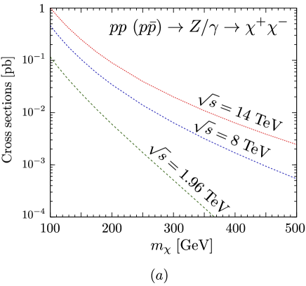
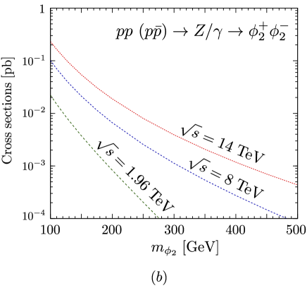
Refer to caption Refer to caption

Figure 13: Pair production cross sections of (a) χ𝜒\chi in case of Qχ=1subscript𝑄𝜒1Q_{\chi}=-1pp(pp¯)Z/γχ+χ𝑝𝑝𝑝¯𝑝𝑍𝛾superscript𝜒superscript𝜒pp~{}(p\bar{p})\rightarrow Z/\gamma\rightarrow\chi^{+}\chi^{-}, and (b) ϕ2superscriptsubscriptitalic-ϕ2\phi_{2}^{-} in case of Q2=1subscript𝑄21Q_{2}=-1pp(pp¯)Z/γϕ2+ϕ2𝑝𝑝𝑝¯𝑝𝑍𝛾superscriptsubscriptitalic-ϕ2superscriptsubscriptitalic-ϕ2pp~{}(p\bar{p})\rightarrow Z/\gamma\rightarrow\phi_{2}^{+}\phi_{2}^{-} at the LHC (Tevatron), as a function of mχsubscript𝑚𝜒m_{\chi} and mϕ2subscript𝑚subscriptitalic-ϕ2m_{\phi_{2}}, respectively. Here we take s=8𝑠8\sqrt{s}=8 TeV and 14 TeV for LHC and 1.96 TeV for Tevatron.

In the case where the right-handed muon has new Yukawa coupling, singlet scalar (ϕitalic-ϕ\phi) and singlet fermion (χ𝜒\chi) exist in the model. When Qχ=1subscript𝑄𝜒1Q_{\chi}=-1, only χ𝜒\chi couples to the standard model gauge bosons (Z𝑍Z and γ𝛾\gamma) because Qϕ=0subscript𝑄italic-ϕ0Q_{\phi}=0. Therefore, the fermion χ𝜒\chi can be pair-produced via EW gauge interactions. We calculate the pair production cross section of χ𝜒\chi at the LHC (s=8TeVand14TeV𝑠8TeVand14TeV\sqrt{s}=8~{}{\rm TeV}~{}{\rm and}~{}14~{}{\rm TeV}) and at Tevatron (s=1.96𝑠1.96\sqrt{s}=1.96 TeV) as a function of mχsubscript𝑚𝜒m_{\chi}, as shown in Fig. 13(a). To calculate the production cross sections, we have used the MadGraph [19]. In order to explain the anomaly of muon g-2, the mass of the fermion χ𝜒\chi should be of order of about 100 GeV. From Fig. 13(a), the production cross section of χ𝜒\chi is in the range of 0.5-0.0005 pb (1-0.001 pb) for mχ=100500subscript𝑚𝜒100500m_{\chi}=100-500 GeV and s=8𝑠8\sqrt{s}=8 TeV (s=14𝑠14\sqrt{s}=14 TeV) at the LHC and also 0.1-0.001 pb for mχ=100250subscript𝑚𝜒100250m_{\chi}=100-250 GeV and s=1.96𝑠1.96\sqrt{s}=1.96 TeV at the Tevatron. If we consider a luminosity of 10 fb-1 for s=8𝑠8\sqrt{s}=8 TeV and 14 TeV, the number of events produced at the LHC is of order of 5-5000 and 10-10000, respectively. Therefore, number of signal events can be significant. In this case, if ϕitalic-ϕ\phi is lighter than χ𝜒\chi, χ𝜒\chi can decay to μ𝜇\mu and ϕitalic-ϕ\phi. If ϕitalic-ϕ\phi is a stable neutral particle, the final signature may be a μ+μsuperscript𝜇superscript𝜇\mu^{+}\mu^{-}+ missing energy. This will suffer from the standard model background such as W+W(μ+μ)annotatedsuperscript𝑊superscript𝑊absentsuperscript𝜇superscript𝜇W^{+}W^{-}(\rightarrow\mu^{+}\mu^{-}) production whose production rate is about 0.29 (0.51) pb for s=8𝑠8\sqrt{s}=8 TeV (14 TeV) at the LHC. Therefore, the detail study will be very important to discuss the discovery potential of such a signal event. However, the detail signature will depend on the particle spectrum in the complete model. Thus we will leave the detail study. If we consider multi-charged χ𝜒\chi, the cross section increases by a factor Qχ2superscriptsubscript𝑄𝜒2Q_{\chi}^{2}, and the cross section further becomes larger, and hence the constraints from the LHC will be very important. #7#7#7In addition, ϕitalic-ϕ\phi pair production is also not negligible in this case.

In the second model where one has a SU(2)L𝑆𝑈subscript2𝐿SU(2)_{L} doublet scalar in addition to ϕitalic-ϕ\phi and χ𝜒\chi, the scalars can be pair-produced via EW gauge interaction. For example, Fig. 13 (b) shows the production cross sections for the charged ϕ2+ϕ2superscriptsubscriptitalic-ϕ2superscriptsubscriptitalic-ϕ2\phi_{2}^{+}\phi_{2}^{-} scalars as a function of mϕ2subscript𝑚subscriptitalic-ϕ2m_{\phi_{2}} in case of Qχ=0subscript𝑄𝜒0Q_{\chi}=0, which corresponds to Q1=0subscript𝑄10Q_{1}=0 and Q2=1subscript𝑄21Q_{2}=-1. We show the predicted values for s=8𝑠8\sqrt{s}=8 TeV and 14 TeV at the LHC and s=1.96𝑠1.96\sqrt{s}=1.96 TeV at the Tevatron. As can be seen from the figure, the cross sections are in the range of 0.1-0.0001 pb (0.2-0.0005 pb) for mϕ2=100500subscript𝑚subscriptitalic-ϕ2100500m_{\phi_{2}}=100-500~{} GeV at s=8𝑠8\sqrt{s}=8 TeV (s=14𝑠14\sqrt{s}=14 TeV) and also 0.02-0.0001 pb for for mϕ2=100250subscript𝑚subscriptitalic-ϕ2100250m_{\phi_{2}}=100-250 GeV at the Tevatron. For simplicity, we have assumed that there are no ϕitalic-ϕ\phi-ϕ2subscriptitalic-ϕ2\phi_{2} scalar mixing. In this case, ϕ1+ϕ2subscriptitalic-ϕ1subscriptitalic-ϕ2\phi_{1}+\phi_{2} are also produced via W𝑊W-boson. If masses of SU(2)L𝑆𝑈subscript2𝐿SU(2)_{L} doublet scalar are degenerated, we have checked that the cross section is similar to one in Fig. 13 (b). In general, the signal events have the form pp(pp¯)Vϕiϕj𝑝𝑝𝑝¯𝑝𝑉subscriptsuperscriptitalic-ϕ𝑖subscriptitalic-ϕ𝑗pp~{}(p\bar{p})\to V\to\phi^{*}_{i}\phi_{j} where V=Z,γ,W𝑉𝑍𝛾𝑊V=Z,\gamma,W and i,j=1,2formulae-sequence𝑖𝑗12i,j=1,2. Therefore, Fig. 13 shows the typical values of the cross section in this model.

Although we can not discuss the complete signatures because our sample models are not complete, we stress that the searches for the production processes of these new particles via EW interactions are very important in models where the anomaly of muon g-2 can be explained by these new particles.

5 Summary

The current LHC experiment does not show any deviation from the SM predictions. This result puts severe constraints on new physics models. Especially, colored particles are strongly constrained since the LHC as a hadron collider can easily produce the colored particles via QCD interactions. For example, in the constrained minimal supersymmetric standard model (CMSSM), gluino as well as the first and the second generation squarks are strongly constrained and their typical lower mass limits are about 1 TeV [20]. Therefore, models motivated by the hierarchy problem are getting more constrained, and especially CMSSM as a solution to the hierarchy problem is strongly disfavored.

If we motivate new physics models from the reported anomaly of muon g-2, our naive expectation is the existence of EW scale new particles because the size of anomaly of muon g-2 is as large as one induced by EW gauge bosons in the SM. In this paper, we analyzed two examples, where muon has new Yukawa type interactions with new particles. One example was a model where right-handed muon has new Yukawa interaction with SU(2) singlet scalar and fermion. In this case, in order to explain the anomaly of muon g-2 as well as to satisfy the precision EW measurements, we found that the relatively large new Yukawa coupling and EW scale new particles are strongly favored. We also noted that the multi-charged particles (whose QED charges are large) are favored.

Another example we analyzed was a model where both right- and left-handed muons have new Yukawa interactions with SU(2) doublet scalar and singlet scalar and fermion, so that the chirality flip of muon can occur in the internal fermion line of 1-loop muon g-2 diagrams. In this case, new contributions to muon g-2 are enhanced, and hence even smaller new Yukawa couplings can explain the anomaly of muon g-2. We also showed that the EW observables are also well-fitted by the new physics contributions. In this case, the EW scale new particles are favored by the data.

Although these two examples may be only a part of complete models, the muon g-2 as well as the EW observables can constrain the QED charge of new particles as well as the scale of new particles and the size of new Yukawa couplings. Since the EW scale new particles can explain the anomaly of muon g-2 and they can be consistent with the precision EW measurements, it is important to study the possible phenomenology at the LHC.

Since some of new particles have QED charges as well as couplings with Higgs boson, the branching ratio of hγγ𝛾𝛾h\rightarrow\gamma\gamma can be effected. Especially, as we showed, multi-charged particles favored by the muon g-2 can significantly contribute to hγγ𝛾𝛾h\rightarrow\gamma\gamma, and the effects can be sizable. Therefore, Higgs physics will have an impact on models we discussed here.

We also computed direct production cross sections of new particles motivated by the muon g-2. Since models discussed here may not be complete, we could not discuss the complete signatures for the models. However, since the number of signal events are not negligible, there may be possibility to reveal new physics models for muon g-2 at the LHC. Since we do not need the colored particles to explain the anomaly of muon g-2, the search for new particles which only have EW interactions will be very important.

Finally, we comment on the possible completions of models discussed in this paper. The structure of the model where both right- and left-handed muons have new Yukawa type interactions is quite similar to that of the minimal supersymmetric standard model. When Q2=1subscript𝑄21Q_{2}=-1, the scalar ϕ2subscriptitalic-ϕ2\phi_{2} in SU(2) doublet scalar ΦΦ\Phi and SU(2) singlet scalar ϕitalic-ϕ\phi correspond to left- and right-handed smuons, respectively. The SU(2) singlet fermion χ𝜒\chi is a Bino, for example. A part of a model discussed in Ref. [21], which is motivated by neutrino mass and dark matter is also similar to the model we discussed here. Therefore, our approach can capture crucial features of new physics models for the anomaly of muon g-2 and hopefully create an interesting way to find the physics beyond the standard model.

Note added

After we completed this work, we learned that ATLAS and CMS collaboration at LHC observed a new particle consistent with the SM Higgs boson at a mass of about 125 GeV [22]. Since we have taken the Higgs boson mass to be 125 GeV in our analysis, our conclusion does not change.

Acknowledgments

This work is supported in part by Grant-in-Aid for Scientific research from the Ministry of Education, Science, Sports, and Culture (MEXT), Japan, No. 22540273 (KT). This work is also supported in part by Grant-in-Aid for Nagoya University Global COE Program, “Quest for Fundamental Principles in the Universe: from Particles to the Solar System and the Cosmos”, from the MEXT, Japan.

Appendix A Useful function

In this paper, Passarino-Veltman functions [9] are defined by

A(A)𝐴𝐴\displaystyle A(A) =\displaystyle= 16π2μ2ϵdnki(2π)n1k2mA2+iϵ,16superscript𝜋2superscript𝜇2italic-ϵsuperscript𝑑𝑛𝑘𝑖superscript2𝜋𝑛1superscript𝑘2superscriptsubscript𝑚𝐴2𝑖italic-ϵ\displaystyle 16\pi^{2}\mu^{2\epsilon}\int\frac{d^{n}k}{i(2\pi)^{n}}\frac{1}{k^{2}-m_{A}^{2}+i\epsilon}, (A.1)
B0(A,B;p)subscript𝐵0𝐴𝐵𝑝\displaystyle B_{0}(A,B;p) =\displaystyle= 16π2μ2ϵdnki(2π)n1[k2mA2+iϵ][(k+p)2mB2+iϵ],16superscript𝜋2superscript𝜇2italic-ϵsuperscript𝑑𝑛𝑘𝑖superscript2𝜋𝑛1delimited-[]superscript𝑘2superscriptsubscript𝑚𝐴2𝑖italic-ϵdelimited-[]superscript𝑘𝑝2superscriptsubscript𝑚𝐵2𝑖italic-ϵ\displaystyle 16\pi^{2}\mu^{2\epsilon}\int\frac{d^{n}k}{i(2\pi)^{n}}\frac{1}{\left[k^{2}-m_{A}^{2}+i\epsilon\right]\left[(k+p)^{2}-m_{B}^{2}+i\epsilon\right]},
pμB1(A,B;p)superscript𝑝𝜇subscript𝐵1𝐴𝐵𝑝\displaystyle p^{\mu}B_{1}(A,B;p) =\displaystyle= 16π2μ2ϵdnki(2π)nkμ[k2mA2+iϵ][(k+p)2mB2+iϵ],16superscript𝜋2superscript𝜇2italic-ϵsuperscript𝑑𝑛𝑘𝑖superscript2𝜋𝑛superscript𝑘𝜇delimited-[]superscript𝑘2superscriptsubscript𝑚𝐴2𝑖italic-ϵdelimited-[]superscript𝑘𝑝2superscriptsubscript𝑚𝐵2𝑖italic-ϵ\displaystyle 16\pi^{2}\mu^{2\epsilon}\int\frac{d^{n}k}{i(2\pi)^{n}}\frac{k^{\mu}}{\left[k^{2}-m_{A}^{2}+i\epsilon\right]\left[(k+p)^{2}-m_{B}^{2}+i\epsilon\right]},
pμpνB21(A,B;p)superscript𝑝𝜇superscript𝑝𝜈subscript𝐵21𝐴𝐵𝑝\displaystyle p^{\mu}p^{\nu}B_{21}(A,B;p) +\displaystyle+ gμνB22(A,B;p)superscript𝑔𝜇𝜈subscript𝐵22𝐴𝐵𝑝\displaystyle g^{\mu\nu}B_{22}(A,B;p) (A.2)
=\displaystyle= 16π2μ2ϵdnki(2π)nkμkν[k2mA2+iϵ][(k+p)2mB2+iϵ],16superscript𝜋2superscript𝜇2italic-ϵsuperscript𝑑𝑛𝑘𝑖superscript2𝜋𝑛superscript𝑘𝜇superscript𝑘𝜈delimited-[]superscript𝑘2superscriptsubscript𝑚𝐴2𝑖italic-ϵdelimited-[]superscript𝑘𝑝2superscriptsubscript𝑚𝐵2𝑖italic-ϵ\displaystyle 16\pi^{2}\mu^{2\epsilon}\int\frac{d^{n}k}{i(2\pi)^{n}}\frac{k^{\mu}k^{\nu}}{\left[k^{2}-m_{A}^{2}+i\epsilon\right]\left[(k+p)^{2}-m_{B}^{2}+i\epsilon\right]},
C0(A,B,C;p1,p2)subscript𝐶0𝐴𝐵𝐶subscript𝑝1subscript𝑝2\displaystyle C_{0}(A,B,C;p_{1},p_{2})
=\displaystyle= 16π2μ2ϵdnki(2π)n1[k2mA2+iϵ][(k+p1)2mB2+iϵ][(k+p1+p2)2mC2+iϵ],16superscript𝜋2superscript𝜇2italic-ϵsuperscript𝑑𝑛𝑘𝑖superscript2𝜋𝑛1delimited-[]superscript𝑘2superscriptsubscript𝑚𝐴2𝑖italic-ϵdelimited-[]superscript𝑘subscript𝑝12superscriptsubscript𝑚𝐵2𝑖italic-ϵdelimited-[]superscript𝑘subscript𝑝1subscript𝑝22superscriptsubscript𝑚𝐶2𝑖italic-ϵ\displaystyle 16\pi^{2}\mu^{2\epsilon}\int\frac{d^{n}k}{i(2\pi)^{n}}\frac{1}{[k^{2}-m_{A}^{2}+i\epsilon][(k+p_{1})^{2}-m_{B}^{2}+i\epsilon][(k+p_{1}+p_{2})^{2}-m_{C}^{2}+i\epsilon]},
(p1μC11+p2μC12)(A,B,C;p1,p2)superscriptsubscript𝑝1𝜇subscript𝐶11superscriptsubscript𝑝2𝜇subscript𝐶12𝐴𝐵𝐶subscript𝑝1subscript𝑝2\displaystyle\left(p_{1}^{\mu}C_{11}+p_{2}^{\mu}C_{12}\right)(A,B,C;p_{1},p_{2})
=\displaystyle= 16π2μ2ϵdnki(2π)nkμ[k2mA2+iϵ][(k+p1)2mB2+iϵ][(k+p1+p2)2mC2+iϵ],16superscript𝜋2superscript𝜇2italic-ϵsuperscript𝑑𝑛𝑘𝑖superscript2𝜋𝑛superscript𝑘𝜇delimited-[]superscript𝑘2superscriptsubscript𝑚𝐴2𝑖italic-ϵdelimited-[]superscript𝑘subscript𝑝12superscriptsubscript𝑚𝐵2𝑖italic-ϵdelimited-[]superscript𝑘subscript𝑝1subscript𝑝22superscriptsubscript𝑚𝐶2𝑖italic-ϵ\displaystyle 16\pi^{2}\mu^{2\epsilon}\int\frac{d^{n}k}{i(2\pi)^{n}}\frac{k^{\mu}}{[k^{2}-m_{A}^{2}+i\epsilon][(k+p_{1})^{2}-m_{B}^{2}+i\epsilon][(k+p_{1}+p_{2})^{2}-m_{C}^{2}+i\epsilon]},
{(p1μp1νC21+p2μp2νC22+(p1μp2ν+p1νp2μ)C23+gμνC24}(A,B,C;p1,p2)\displaystyle\left\{(p_{1}^{\mu}p_{1}^{\nu}C_{21}+p_{2}^{\mu}p_{2}^{\nu}C_{22}+(p_{1}^{\mu}p_{2}^{\nu}+p_{1}^{\nu}p_{2}^{\mu})C_{23}+g^{\mu\nu}C_{24}\right\}(A,B,C;p_{1},p_{2})
=\displaystyle= 16π2μ2ϵdnki(2π)nkμkν[k2mA2+iϵ][(k+p1)2mB2+iϵ][(k+p1+p2)2mC2+iϵ],16superscript𝜋2superscript𝜇2italic-ϵsuperscript𝑑𝑛𝑘𝑖superscript2𝜋𝑛superscript𝑘𝜇superscript𝑘𝜈delimited-[]superscript𝑘2superscriptsubscript𝑚𝐴2𝑖italic-ϵdelimited-[]superscript𝑘subscript𝑝12superscriptsubscript𝑚𝐵2𝑖italic-ϵdelimited-[]superscript𝑘subscript𝑝1subscript𝑝22superscriptsubscript𝑚𝐶2𝑖italic-ϵ\displaystyle 16\pi^{2}\mu^{2\epsilon}\int\frac{d^{n}k}{i(2\pi)^{n}}\frac{k^{\mu}k^{\nu}}{[k^{2}-m_{A}^{2}+i\epsilon][(k+p_{1})^{2}-m_{B}^{2}+i\epsilon][(k+p_{1}+p_{2})^{2}-m_{C}^{2}+i\epsilon]},

where we use dimensional regularization in 42ϵ42italic-ϵ4-2\epsilon dimensions.

For convenience, we list explicit forms of some of above functions.

A(m2)𝐴superscript𝑚2\displaystyle A(m^{2}) =\displaystyle= m2(1Δ+1logm2μ2),superscript𝑚21Δ1superscript𝑚2superscript𝜇2\displaystyle m^{2}\left(\frac{1}{\Delta}+1-\log\frac{m^{2}}{\mu^{2}}\right), (A.4)
B0(A,B;p)subscript𝐵0𝐴𝐵𝑝\displaystyle B_{0}(A,B;p) =\displaystyle= 1Δ01𝑑xlogm12(1x)+m22xp2x(1x)iϵμ2,1Δsuperscriptsubscript01differential-d𝑥superscriptsubscript𝑚121𝑥superscriptsubscript𝑚22𝑥superscript𝑝2𝑥1𝑥𝑖italic-ϵsuperscript𝜇2\displaystyle\frac{1}{\Delta}-\int_{0}^{1}dx\log\frac{m_{1}^{2}(1-x)+m_{2}^{2}x-p^{2}x(1-x)-i\epsilon}{\mu^{2}}, (A.5)
B1(A,B;p)subscript𝐵1𝐴𝐵𝑝\displaystyle B_{1}(A,B;p) =\displaystyle= 12Δ+01𝑑xxlogm12(1x)+m22xp2x(1x)iϵμ2,12Δsuperscriptsubscript01differential-d𝑥𝑥superscriptsubscript𝑚121𝑥superscriptsubscript𝑚22𝑥superscript𝑝2𝑥1𝑥𝑖italic-ϵsuperscript𝜇2\displaystyle-\frac{1}{2\Delta}+\int_{0}^{1}dxx\log\frac{m_{1}^{2}(1-x)+m_{2}^{2}x-p^{2}x(1-x)-i\epsilon}{\mu^{2}}, (A.6)
B21(A,B;p)subscript𝐵21𝐴𝐵𝑝\displaystyle B_{21}(A,B;p) =\displaystyle= 13Δ01𝑑xx2logm12(1x)+m22xp2x(1x)iϵμ2,13Δsuperscriptsubscript01differential-d𝑥superscript𝑥2superscriptsubscript𝑚121𝑥superscriptsubscript𝑚22𝑥superscript𝑝2𝑥1𝑥𝑖italic-ϵsuperscript𝜇2\displaystyle\frac{1}{3\Delta}-\int_{0}^{1}dxx^{2}\log\frac{m_{1}^{2}(1-x)+m_{2}^{2}x-p^{2}x(1-x)-i\epsilon}{\mu^{2}}, (A.7)
B22(A,B;p)subscript𝐵22𝐴𝐵𝑝\displaystyle B_{22}(A,B;p) =\displaystyle= 14(m12+m22p23)(1Δ+1)14superscriptsubscript𝑚12superscriptsubscript𝑚22superscript𝑝231Δ1\displaystyle\frac{1}{4}(m_{1}^{2}+m_{2}^{2}-\frac{p^{2}}{3})\left(\frac{1}{\Delta}+1\right) (A.8)
1201𝑑x{m12(1x)+m22xp2x(1x)}logm12(1x)+m22xp2x(1x)iϵμ2,12superscriptsubscript01differential-d𝑥superscriptsubscript𝑚121𝑥superscriptsubscript𝑚22𝑥superscript𝑝2𝑥1𝑥superscriptsubscript𝑚121𝑥superscriptsubscript𝑚22𝑥superscript𝑝2𝑥1𝑥𝑖italic-ϵsuperscript𝜇2\displaystyle-\frac{1}{2}\int_{0}^{1}dx\left\{m_{1}^{2}(1-x)+m_{2}^{2}x-p^{2}x(1-x)\right\}\log\frac{m_{1}^{2}(1-x)+m_{2}^{2}x-p^{2}x(1-x)-i\epsilon}{\mu^{2}},

where 1Δ=1ϵγ+log4π1Δ1italic-ϵ𝛾4𝜋\frac{1}{\Delta}=\frac{1}{\epsilon}-\gamma+\log 4\pi.

References

  • [1] G. Aad et al. [ATLAS Collaboration], Phys. Lett. B 710, 49 (2012) [arXiv:1202.1408]; S. Chatrchyan et al. [CMS Collaboration], arXiv:1202.1488. See also recent Tevatron result; [TEVNPH (Tevatron New Phenomina and Higgs Working Group) and CDF and D0 Collaborations], arXiv:1203.3774.
  • [2] K. Nakamura et al. [Particle Data Group Collaboration], J. Phys. G G 37, 075021 (2010); B. L. Roberts, Chin. Phys. C 34, 741 (2010) [arXiv:1001.2898].
  • [3] K. Hagiwara et al., J. Phys. G G 38, 085003 (2011) [arXiv:1105.3149]. See also F. Jegerlehner and A. Nyffeler, Phys. Rept.  477, 1 (2009) [arXiv:0902.3360]; M. Davier et al., Eur. Phys. J. C 71, 1515 (2011) [Erratum-ibid. C 72, 1874 (2012)] [arXiv:1010.4180]; F. Jegerlehner and R. Szafron, Eur. Phys. J. C 71, 1632 (2011) [arXiv:1101.2872]; T. Teubner et al., AIP Conf. Proc.  1343, 340 (2011); Nucl. Phys. Proc. Suppl.  218, 225 (2011).
  • [4] T. Aoyama et al., arXiv:1205.5370; arXiv:1205.5368; R. Boughezal and K. Melnikov, Phys. Lett. B 704, 193 (2011) [arXiv:1104.4510]; A. E. Dorokhov, A. E. Radzhabov and A. S. Zhevlakov, Eur. Phys. J. C 71, 1702 (2011) [arXiv:1103.2042]; T. Goecke, C. S. Fischer and R. Williams, Phys. Rev. D 83, 094006 (2011) [arXiv:1012.3886]; Eur. Phys. J. A 47, 28 (2011) [arXiv:1009.5297]; A. Nyffeler, Chin. Phys. C 34, 705 (2010) [arXiv:1001.3970]; A. Nyffeler, Phys. Rev. D 79, 073012 (2009) [arXiv:0901.1172]; D. K. Hong and D. Kim, Phys. Lett. B 680, 480 (2009) [arXiv:0904.4042]; J. Prades, E. de Rafael and A. Vainshtein, [arXiv:0901.0306]; A. E. Dorokhov and W. Broniowski, Phys. Rev. D 78, 073011 (2008) [arXiv:0805.0760]; J. Bijnens and J. Prades, Mod. Phys. Lett. A 22, 767 (2007) [hep-ph/0702170]; M. Hayakawa et al., PoS LAT 2005, 353 (2006) [hep-lat/0509016]; K. Melnikov and A. Vainshtein, Phys. Rev. D 70, 113006 (2004) [hep-ph/0312226]; J. H. Kuhn, A. I. Onishchenko, A. A. Pivovarov and O. L. Veretin, Phys. Rev. D 68, 033018 (2003) [hep-ph/0301151]; T. Kinoshita and M. Nio, Phys. Rev. Lett.  90, 021803 (2003) [hep-ph/0210322]; M. J. Ramsey-Musolf and M. B. Wise, Phys. Rev. Lett.  89, 041601 (2002) [hep-ph/0201297]; J. Bijnens, E. Pallante and J. Prades, Nucl. Phys. B 626, 410 (2002) [hep-ph/0112255]; Nucl. Phys. B 474, 379 (1996) [hep-ph/9511388]; J. Bijnens, E. Pallante and J. Prades, Phys. Rev. Lett.  75, 1447 (1995) [Erratum-ibid.  75, 3781 (1995)] [hep-ph/9505251]; I. R. Blokland, A. Czarnecki and K. Melnikov, Phys. Rev. Lett.  88, 071803 (2002) [hep-ph/0112117]; M. Knecht, A. Nyffeler, M. Perrottet and E. de Rafael, Phys. Rev. Lett.  88, 071802 (2002) [hep-ph/0111059]; M. Knecht and A. Nyffeler, Phys. Rev. D 65, 073034 (2002) [hep-ph/0111058]; Z. Bern, A. De Freitas, L. J. Dixon, A. Ghinculov and H. L. Wong, JHEP 0111, 031 (2001) [hep-ph/0109079]; M. Hayakawa and T. Kinoshita, Phys. Rev. D 57, 465 (1998) [Erratum-ibid. D 66, 019902 (2002)] [hep-ph/9708227]; M. Hayakawa, T. Kinoshita and A. I. Sanda, Phys. Rev. D 54, 3137 (1996) [hep-ph/9601310]; M. Hayakawa, T. Kinoshita and A. I. Sanda, Phys. Rev. Lett.  75, 790 (1995) [hep-ph/9503463].
  • [5] T. Moroi, Phys. Rev. D 53, 6565 (1996) [Erratum-ibid. D 56, 4424 (1997)] [hep-ph/9512396].
  • [6] G. C. McLaughlin and J. N. Ng, Phys. Lett. B 493, 88 (2000) [hep-ph/0008209].
  • [7] S. R. Choudhury, A. S. Cornell, A. Deandrea, N. Gaur and A. Goyal, Phys. Rev. D 75, 055011 (2007) [hep-ph/0612327].
  • [8] K. Kannike, M. Raidal, D. M. Straub and A. Strumia, JHEP 1202, 106 (2012) [arXiv:1111.2551]; H. Davoudiasl, H. -S. Lee and W. J. Marciano, arXiv:1205.2709.
  • [9] G. ’t Hooft and M. J. G. Veltman, Nucl. Phys. B 153, 365 (1979); G. Passarino and M. J. G. Veltman, Nucl. Phys. B 160, 151 (1979).
  • [10] G. -C. Cho et al., JHEP 1111, 068 (2011) [arXiv:1104.1769].
  • [11] G. -C. Cho and K. Hagiwara, Nucl. Phys. B 574, 623 (2000) [hep-ph/9912260].
  • [12] K. Hagiwara et al., Z. Phys. C 64, 559 (1994) [Erratum-ibid. C 68, 352 (1995)] [hep-ph/9409380].
  • [13] M. E. Peskin and T. Takeuchi, Phys. Rev. Lett.  65, 964 (1990); Phys. Rev. D 46, 381 (1992).
  • [14] G. Altarelli and R. Barbieri, Phys. Lett. B 253, 161 (1991); G. Altarelli, R. Barbieri and S. Jadach, Nucl. Phys. B 369, 3 (1992) [Erratum-ibid. B 376, 444 (1992)]; G. Altarelli, R. Barbieri and F. Caravaglios, Phys. Lett. B 349, 145 (1995).
  • [15] I. Maksymyk, C. P. Burgess and D. London, Phys. Rev. D 50, 529 (1994) [hep-ph/9306267].
  • [16] Tevatron Electroweak Working Group, f. t. C. Collaboration and D. Collaboration, arXiv:1204.0042.
  • [17] Tevatron Electroweak Working Group and for the CDF and D0 Collaborations, arXiv:1107.5255.
  • [18] See web page: http://lepewwg.web.cern.ch/LEPEWWG/
  • [19] J. Alwall et al., JHEP 0709, 028 (2007) [arXiv:0706.2334].
  • [20] For example, see G. Aad et al. [ATLAS Collaboration], arXiv:1206.1760; S. Chatrchyan et al. [CMS Collaboration], arXiv:1206.3949.
  • [21] T. Hambye, K. Kannike, E. Ma and M. Raidal, Phys. Rev. D 75, 095003 (2007) [hep-ph/0609228].
  • [22] G. Aad et al. [ATLAS Collaboration], [arXiv:1207.7214]; S. Chatrchyan et al. [CMS Collaboration], Phys. Lett. B [arXiv:1207.7235].