Abstract

We present the first determination of parton distributions of the nucleon at NLO and NNLO based on a global data set which includes LHC data: NNPDF2.3. Our data set includes, besides the deep inelastic, Drell-Yan, gauge boson production and jet data already used in previous global PDF determinations, all the relevant LHC data for which experimental systematic uncertainties are currently available: ATLAS and LHCb W and Z rapidity distributions from the 2010 run, CMS W electron asymmetry data from the 2011 run, and ATLAS inclusive jet cross-sections from the 2010 run. We introduce an improved implementation of the FastKernel method which allows us to fit to this extended data set, and also to adopt a more effective minimization methodology. We present the NNPDF2.3 PDF sets, and compare them to the NNPDF2.1 sets to assess the impact of the LHC data. We find that all the LHC data are broadly consistent with each other and with all the older data sets included in the fit. We present predictions for various standard candle cross-sections, and compare them to those obtained previously using NNPDF2.1, and specifically discuss the impact of ATLAS electroweak data on the determination of the strangeness fraction of the proton. We also present collider PDF sets, constructed using only data from HERA, Tevatron and LHC, but find that this data set is neither precise nor complete enough for a competitive PDF determination.

1 Introduction

The most accurate available information on the parton distribution functions (PDFs) of the nucleon, an essential ingredient for hadron collider phenomenology [1, 2, 3], comes from global fits to extended sets of data obtained from a variety of different electro- and hadroproduction processes, in particular, deep inelastic scattering (DIS), Drell-Yan (DY) and gauge boson production, and jet production. The combination of the information from all these processes allows one to determine six independent light quark and antiquark distributions and the gluon. Data from the LHC are likely to offer very significant improvements in the accuracy of these determinations, because of their greater precision and kinematic coverage, and also because of the greater range of precise cross-sections available, including processes such as gauge boson production in association with jets and charm which hitherto have not been used for PDF determinations.

In fact, data for processes relevant for PDF determination collected at the LHC during the first run in 2010 already reached an accuracy comparable to pre-existing data. In Ref. [4, 5] we presented a first study of the impact on PDFs of LHC data, specifically the $36~{}{\rm pb}^{-1}$ W-lepton asymmetry data from ATLAS and CMS, then available without full information on correlated systematics. We constructed a PDF set, NNPDF2.2, by reweighting [6] the NNPDF2.1 NLO and NNLO PDF sets [7, 8]. Even with the modest amount of new experimental information then available, small improvements in the accuracy and changes in the shape of light-quark distributions in the medium and small $x$ region were found.

Meanwhile, several LHC data sets with full information on correlated systematics have been published, in particular gauge boson production data from ATLAS, CMS and LHCb, and inclusive jet and dijet data from ATLAS. Preliminary studies [9] with some of these data have shown that, thanks to the information on correlated systematics, their impact on PDFs is significant: if included by reweighting the NNPDF2.1 set, one has to start with a large number of replicas in order to obtain accurate results. A new set of PDFs including this considerable amount of new information is thus needed, with the new data included in the fit, rather than added at a second stage via reweighting.

It is the purpose of this paper to present such a PDF determination, using the methodology developed by the NNPDF collaboration [10, 11, 12, 13, 14, 15, 16, 17], and used to produce the NNPDF2.1 LO, NLO, and NNLO PDF sets [7, 8] which are now part of the PDF4LHC prescription [18] for reliable determination of PDF uncertainties in LHC processes. The new PDF set presented here, NNPDF2.3, is the most accurate determination to date from the NNPDF family, and it supersedes previous existing sets. It differs from the NNPDF2.1 set because of the inclusion of LHC data, and also because of some improvements in fitting methodology, specifically in the genetic algorithm which is used to determine the fit to the replicas.

We will determine NNPDF2.3 PDFs both at NLO and NNLO for a wide range of values of $\alpha_{s}$, so that the user can select their own preferred value. While the default NNPDF sets use a variable-flavor number general-mass scheme based on the FONLL [19, 20, 21] method for the inclusion of heavy quark masses, in which the number of active flavor increases at each quark threshold, we also provide PDF sets in which the maximum number of active flavors is fixed at $n_{f}=4$ or $n_{f}=5$, which may be useful for specific applications (see for example Refs.[22, 23]). We will also provide NNPDF2.3 NLO and NNLO sets based on reduced data sets: an NNPDF2.3 noLHC set, which uses exactly the same data set as NNPDF2.1, and differs from it only because of the improved methodology; and an NNPDF2.3 collider set, which only uses HERA inclusive and charm DIS data, Tevatron gauge boson production and jet data, and LHC data, and excludes all fixed target data. The former set is useful for the precise assessment of the impact of LHC data, and also if one for some reason wishes to avoid using LHC data, for example for unbiased new physics searches at LHC. The latter set is interesting because the fixed-target data, both for DIS and DY, are problematic: they are generally at lower scales (hence many of them are potentially subject to indeterminate higher-twist corrections), some carry no information on correlated systematics, and finally many of them (such as NMC and BCDMS and all neutrino DIS data, and Tevatron DY data) are partly or fully obtained using nuclear targets which may be subject to significant but unknown nuclear corrections. Jet data, which are affected by larger theoretical uncertainties, play at present a relatively minor role, so a collider-only fit is at present definitely theoretically rather more reliable than the global fit: unfortunately we find that it is not yet competitive in terms of statistical precision.

The paper is organized as follows. In Sec. 2 we will summarize the general features of the LHC data which are being added to the data set, and specifically the choices of kinematic cuts. In Sec. 3 we will discuss the methodological improvements which are being introduced in the NNPDF2.3 determination. In order to cope with the non-negligible widening of the data set — the number of data for hadron collider processes, which are computationally the most intensive since they depend quadratically on the PDFs, is considerably increased in comparison to NNPDF2.1 — we introduce here (Sec. 3.1–3.2) a new, more efficient implementation of our previous FastKernel method [17] for the computation of hadronic observables. The ensuing considerable improvement in computational efficiency allows us to switch to a new choice of settings for the genetic algorithm which is used for minimization, which is computationally rather more intensive but leads to more precise results (Sec. 3.3). In Sec. 4 we discuss the NNPDF2.3 PDF set: after summarizing the statistical features of the fit, we present the PDFs, and compare them to our previous NNPDF2.1 set, specifically by separating the effect of the LHC data and that of the improved methodology, through a comparison which also involves the NNPDF2.3 noLHC set. The analysis of the impact of LHC data is expanded upon in Sec. 5. First, we determine quantitatively through the reweighting technique the amount of information introduced in the fit by LHC data and their degree of consistency with the rest of the data set, and examine how the description of the LHC data improves when they are included in the fit. Then, we study in detail the compatibility of collider data (including those from the LHC) with fixed target data. Finally, we specifically address the issue of the amount of strangeness in the nucleon, which has attracted some attention recently [24], and in particular show that even though ATLAS data seem to favour a somewhat larger strange fraction, once uncertainties are properly accounted for there is no incompatibility between ATLAS and fixed target data. Finally, in Sec. 6, after briefly discussing NNPDF2.3 parton luminosities, we compare several standard candle cross-sections obtained with them to those obtained with NNPDF2.1.

2 Experimental data

In this section we describe the data set used in the NNPDF2.3 analysis. The non-LHC data is the same as in the corresponding NNPDF2.1 NLO and NNLO fits: this includes NMC [25, 26], BCDMS [27, 28] and SLAC [29] deep inelastic scattering (DIS) fixed target data; the combined HERA-I DIS data set [30], HERA $F_{L}$ [31] and $F_{2}^{c}$ structure function data [32, 33, 34, 35, 36, 37, 38], ZEUS HERA-II DIS cross-sections [39, 40], CHORUS inclusive neutrino DIS [41], and NuTeV dimuon production data [42, 43]; fixed-target E605 [44] and E866 [45, 46, 47] Drell-Yan production data; CDF W asymmetry [48] and CDF [49] and D0 [50] Z rapidity distributions; and CDF [51] and D0 [52] Run-II one-jet inclusive cross-sections. The kinematical cuts are unchanged from NNPDF2.1, so we will not review these data sets here. Instead we will focus on the features of the LHC data included in NNPDF2.3. First we discuss electroweak gauge boson production and then inclusive jets. In each case we describe the NLO and NNLO codes and the corresponding settings used to compute the theoretical predictions for each of these data sets, while in the next section we describe the practical implementation of these calculations into the FastKernel method used in the NNPDF fitting code.

The LHC has already provided an impressive set of measurements which are sensitive to parton distributions, mostly from the 2010 run based on a total integrated luminosity of $36~{}{\rm pb}^{-1}$: the inclusive jet and dijet data [53, 54, 55], electroweak vector boson production [56, 57, 58, 59, 60, 61], both inclusive and in association with heavy quarks [62], and direct photon production, both inclusive and associated with jets [63, 64, 65]. Several other measurements from the 2011 and 2012 runs, which are very relevant for PDF fits, will be available in the next months, like the CMS and LHCb low mass Drell-Yan differential distributions [66, 67] and the inclusive jets and dijets from ATLAS and CMS [68].

Precise determination of PDFs, adequate to current needs, requires the use of experimental data which come with a full covariance matrix. In NNPDF2.3 we include all currently available LHC data for which the experimental covariance matrix has been provided: the ATLAS W and Z lepton rapidity distributions from the 2010 data set, the CMS W electron asymmetry from the 2011 data set and the LHCb W lepton rapidity distributions from the 2010 data set [61], together with the ATLAS inclusive jet cross-sections from the 2010 run [55].

Tevatron Run II lepton asymmetry data from W production were included in Ref. [6] by reweighting the NNPDF2.0 PDF set. Some of these data had issues of compatibility with the rest of the NNPDF2.0-NNPDF2.1 dataset (these two PDF sets only differ in the treatment of heavy quark mass terms), and they only had a moderate impact on PDF uncertainty and essentially no effect on the PDF shape. We prefer therefore not to include these data in the NNPDF2.3 set, and concentrate on the impact of LHC data.

Also, for the time being we do not increase the set of physical processes which are being used for PDF determination. In particular, we choose to use the inclusive jet rather than the dijet cross-sections from ATLAS: to use both would be double counting because they share the same underlying raw data. In principle, dijets cross-sections carry more detailed information on the underlying parton kinematics; however, they are subject to significant scale uncertainties (see for example Ref. [69] and references therein). In the future, as more data with full systematics becomes available, it is likely that the inclusion of new processes in PDF determination will be advantageous. This will require the development of suitable fast interfaces for these processes. An example is prompt photon production, whose impact on the gluon determination was studied recently in Ref. [70].

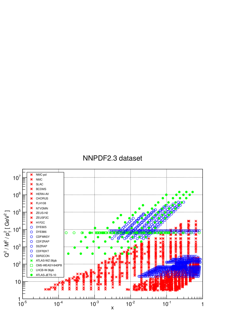
The kinematical coverage of the LHC data sets included in the NNPDF2.3 analysis with the corresponding average experimental uncertainties for each data set are summarized in Tab. 1.. A scatter plot of the kinematical plane for all experimental data from NNPDF2.3 is shown in Fig. 1. The LHC electroweak data span a larger range in Bjorken-$x$ than the Tevatron data thanks to the extended rapidity coverage (up to $\eta=4.5$), while the inclusive jets span a much wider kinematical range both in $x$ and $Q^{2}$ than the one accessible at the Tevatron.

In Tab. 2 we also give the total number of data points used for PDF fitting, both for the NLO and the NNLO global sets, and for the various other PDF sets discussed in Sec. 4. Note that the NLO and NNLO noLHC data sets differ from those of the NNPDF2.1 NLO and NNLO fits of Refs. [7, 8] because of the inclusion in the NNPDF2.3 data set of three NMC data points which were inadvertently neglected in the NNPDF2.1 fits.

Figure 1: The kinematical coverage of the experimental data used in the NNPDF2.3 PDF determination.

Data Set	Ref.	$N_{\rm dat}$	$\left[\eta_{\rm min},\eta_{\rm max}\right]$	$\left\langle\sigma_{\rm stat}\right\rangle$ (%)	$\left\langle\sigma_{\rm sys}\right\rangle$ (%)	$\left\langle\sigma_{\rm norm}\right\rangle$ (%)
CMS W electron asy $840~{}{\rm pb}^{-1}$	[58]	11	$\left[0,2.4\right]$	2.1	4.7	0
ATLAS ${\rm W}^{+}$ $36~{}{\rm pb}^{-1}$	[56]	11	$\left[0,2.4\right]$	1.4	1.3	3.4
ATLAS ${\rm W}^{-}$ $36~{}{\rm pb}^{-1}$	[56]	11	$\left[0,2.4\right]$	1.6	1.4	3.4
ATLAS Z $36~{}{\rm pb}^{-1}$	[56]	8	$\left[0,3.2\right]$	2.8	2.4	3.4
LHCb ${\rm W}^{+}$ $36~{}{\rm pb}^{-1}$	[61]	5	$\left[2,4.5\right]$	4.7	11.1	3.4
LHCb ${\rm W}^{-}$ $36~{}{\rm pb}^{-1}$	[61]	5	$\left[2,4.5\right]$	3.4	7.8	3.4
ATLAS Inclusive Jets 36 pb-1	[55]	90	$\left[0,4.5\right]$	10.2	23.4	3.4

Table 1: The number of data points, kinematical coverage and average statistical, systematic and normalization percentage uncertainties for each of the experimental LHC data sets considered for the NNPDF2.3 analysis. ATLAS inclusive jets refers to the $R=0.4$ data set. There are $146$ LHC data points altogether.

Fit	NLO	NNLO
NNPDF2.3 noLHC	3341	3360
NNPDF2.3 Collider only	1212	1231
NNPDF2.3	3482	3501

Table 2: Total number of data points for the various global sets used for PDF fitting.

2.1 Electroweak boson production

ATLAS has measured the W lepton and Z rapidity distributions from $36~{}{\rm pb}^{-1}$, and provides the full experimental covariance matrix [56]. This measurement supersedes the original muon asymmetry measurement from W decays [57], for which the covariance matrix was not available, and also adds the Z rapidity distributions, which are closely tied to the W lepton distributions by the cross-correlated systematic uncertainties. The CMS collaboration has presented a measurement of the electron asymmetry with $840{\rm pb}^{-1}$ [58] which supersedes the $36~{}{\rm pb}^{-1}$ data [59] and also provides the experimental covariance matrix. CMS has presented a measurement of the normalized Z rapidity distribution with $36~{}{\rm pb}^{-1}$ [60], but the covariance matrix is not available. Finally, the LHCb Collaboration has presented results for the W and Z lepton rapidity distribution, from the 2010 data set [61], again with the experimental covariance matrix; however the $Z$ data are not included in our determination because they are in the process of being reanalyzed [71].

The theoretical predictions for LHC electroweak boson production have been computed at NLO with MCFM [72, 73] interfaced with the APPLgrid library for fast NLO calculations [74]. As discussed in Ref. [8] (see in particular Sec. 3.2) NNLO predictions are obtained by means of local $K$-factors. These have been computed using the DYNNLO code [75], and are found to be quite small, of order 2% at most, and slowly varying with the lepton rapidity.

The calculation of NLO cross-sections requires the implementation of cuts on the lepton kinematics. For the ATLAS data, these are the following:

• cuts for the W lepton rapidity distributions

  $$\centering p_{T}^{l}\geq 20~{}{\rm GeV},\qquad p_{T}^{\nu}\geq 25~{}{\rm GeV},\qquad m_{T}>40~{}{\rm GeV},\qquad|\eta_{l}|\leq 2.5;\@add@centering$$

• cuts for the Z rapidity distribution

  $$p_{T}^{l}\geq 20~{}{\rm GeV},\qquad 66~{}{\rm GeV}\leq m_{l^{+}l^{-}}\leq 116~{}{\rm GeV},\qquad\eta_{l^{+},l^{-}}\leq 4.9.$$

ATLAS measures separately the rapidity distributions in both the electron and muon channels, and then combines them into a common data set. The above kinematical cuts correspond to the combination of electrons and muons, but differ from the cuts applied in individual leptonic channels. For Z rapidity distributions we have explicitly verified that results are unchanged if the cut on the rapidity of the leptons from the Z decay is removed.

For the CMS W electron asymmetry, the only cut is

$$\centering p_{T}^{e}\geq 35~{}{\rm GeV},\@add@centering$$

with the same binning in electron rapidity as in Ref. [58].

Finally, for the LHCb W data the kinematical cuts are

$$\centering p_{T}^{\mu}\geq 20~{}{\rm GeV},\qquad 2.0\leq\eta^{\mu}\leq 4.5.\@add@centering$$

For all three data sets, we performed extensive cross-checks at NLO using two different codes, DYNNLO and MCFM: we checked that, once common settings are adopted, the results of the MCFM and DYNNLO runs agree to better than 1% for all the data bins. An even more accurate agreement could be reached in principle [76], but it is computationally very costly and unnecessary for our purposes. In the particular case of the ATLAS W and Z distributions, we also found good agreement with the APPLgrid tables used in the recent HERAfitter analysis of ATLAS data [24].

2.2 Inclusive jet production

The Tevatron jet data play an important role in constraining the gluon distribution. The kinematics coverage of this constraint is extended considerably by the LHC jet data. From the 2010 $36{\rm pb}^{-1}$ data set inclusive jet and dijet production have been measured by CMS [53, 54] and ATLAS [55], however only ATLAS give the full experimental covariance matrix. The covariance matrix is particularly important for these data because they are highly correlated.

The theoretical calculation of jet production cross-sections in hadron collisions can be carried out by exclusive parton level Monte Carlo codes such as NLOjet++ [77] and EKS-MEKS [78, 79]. More recently, the NLO calculation matched to parton showers in the context of the POWHEG framework has also become available [80], allowing direct hadron level comparisons between theory and data. On the other hand, the full NNLO corrections to the inclusive jet production are unknown, and only the threshold corrections to the inclusive jet $p_{T}$ distribution are available [81], thus the inclusion of jet data into an NNLO analysis is necessarily approximate. Hadron collider jet production data can be consistently included at NLO within a global PDF analysis framework using fast NLO grid codes such as FastNLO [82, 83] or APPLgrid [74].

We compute inclusive jet cross-sections using NLOjet++ interfaced to APPLgrid. The jet reconstruction parameters are identical to those used in the experimental analysis [84]. The NLO calculation uses the anti-$k_{T}$ algorithm [85], and the factorization and renormalization scales are set to be $p_{T}^{\rm max}$, the transverse momentum of the hardest jet in each event. We choose to include in the analysis the data with $R=0.4$. These data are less sensitive to nonperturbative corrections from the underlying event and pileup as compared to the $R=0.6$ data [86, 87], and though they are a bit more sensitive to hadronization effects, all in all the nonperturbative parton to hadron correction factors are smaller for $R=0.4$ than for $R=0.6$. We have checked that the results are essentially unchanged, both in terms of impact on PDFs and at the level of the $\chi^{2}$ description if the $R=0.6$ data is used instead of the $R=0.4$ data.

On top of the 86 sources of fully correlated systematic errors, the ATLAS jet spectra have an additional source of uncertainty due to the theoretical uncertainty in the computation of the hadron to parton nonperturbative correction factors. We take these nonperturbative corrections and their associated uncertainties from the ATLAS analysis, where they are obtained from the variations of different leading order Monte Carlo programs. It is clear from Ref. [84] that for a given Monte Carlo model the nonperturbative correction is strongly correlated between data bins, and thus conservatively we treat it as an additional source of fully correlated systematic uncertainty, to be added to the covariance matrix.

Because NNLO corrections to jet cross-sections are not available, hadron collider jet data can only be included in a NNLO fit within some approximations. As in NNPDF2.1, NNLO theoretical predictions for CDF and D0 inclusive jet data are obtained using the approximate NNLO matrix element obtained from threshold resummation [81] as implemented in the FastNLO framework [82, 83]. For ATLAS data the threshold approximation is expected to be worse because of the higher centre-of-mass energy, and thus we simply used the NLO matrix element with NNLO PDFs and $\alpha_{s}$. It was checked in Ref. [8] that, for Tevatron data, the difference between fits with approximate NNLO jet matrix elements, and fits with purely NLO matrix elements is significantly smaller than the difference between fits with and without jet data.

3 Methodological improvements

We discuss some methodological improvements introduced in the current NNPDF release. First, we present a new efficient method which has allowed us to speed up considerably the computation of hadronic observables while maintaining full NLO accuracy for all experimental data. As explained below, it is a refinement of the FastKernel method introduced in Ref. [17]. The rest of the section describes some improvements of the minimization algorithm, which allow for a more extensive exploration of the space of parameters, and thus a more accurate minimization. These new settings are computationally more intensive, and are made possible by the new implementation of the FastKernel method.

3.1 The FastKernel method revisited: deep inelastic scattering

We first briefly review the FastKernel method in the simplest case of deep inelastic scattering, closely following the original description of the algorithm in Ref. [17]. In the FastKernel method the PDFs at the initial scale $Q_{0}^{2}$ are transformed into the evolution basis [13], in which all nonsinglet combinations decouple, and only the singlet and gluon evolve, coupled to each other. The basis of parametrized PDFs is trivially related to the evolution basis through a linear transformation. The PDFs in the evolution basis at the initial scale are denoted by $N^{0}_{i}(x)$. The index $i$ ranges from 1 to $N_{\rm pdf}=13$, though only the light PDFs are independently parametrized, heavy quarks being generated dynamically during the perturbative evolution. Observables are denoted by $\sigma_{I}$, where $I$ is an index that runs over the number of data points included in the fit. Each data point $\sigma_{I}$ is characterized by a set of kinematic variables. For a DIS observable the kinematic variables characterizing the data points are $(x_{I},Q_{I}^{2})$, and the observable itself can be written as

$$\sigma_{I}=\sum_{i=1}^{N_{\mathrm{pdf}}}K^{I}_{i}\otimes N^{0}_{i}\,,$$ (1)

where $K^{I}_{i}$ is a kernel obtained by convoluting the coefficient functions $C^{I}_{j}$ for $\sigma_{I}$ with the DGLAP evolution kernels $\Gamma_{ji}$, so

$$K^{I}_{i}(x_{I},\alpha_{s}(Q^{2}),\alpha_{s}(Q_{0}^{2}))=\sum_{j=1}^{N_{\rm pdf}}C^{I}_{j}\otimes\Gamma_{ji}(x_{I},\alpha_{s}(Q^{2}),\alpha_{s}(Q_{0}^{2}))\,.$$ (2)

The idea behind the FastKernel method is to approximate the PDFs at the initial scale by a linear combination of interpolating functions

$$N^{0}_{i}(x)=\sum_{\alpha=1}^{N_{x}}N^{0}_{\alpha i}\mathcal{I}^{(\alpha)}(x)\,.$$ (3)

The coefficients of the linear combination are given by the value of the function $N^{0}_{j}(x)$ computed on a grid of points, $N^{0}_{\alpha i}\equiv N^{0}_{i}(x_{\alpha})$. The index $\alpha$ runs from 1 to $N_{x}$, the number of points in the $x$-grid. The same grid of $x$ values is used for all data points $I$. More details on the choice of the grid, and of the interpolating functions can be found in Ref. [17], where the choices that guarantee an accurate interpolation at a sensible computational cost are described. The idea of expanding PDFs in terms of a basis of interpolating polynomials in order to perform PDF evolution more efficiently is the same as that used in the evolution programmes HOPPET [88] and QCDNUM [89]. Using the interpolated PDFs, and writing explicitly the convolution in Eq. (1) yields

$$\sigma_{I}=\sum_{i=1}^{N_{\mathrm{pdf}}}\sum_{\alpha=1}^{N_{x}}\Big{(}\int_{x_{I}}^{1}{{dy}\over{y}}K^{I}_{i}\left({{x_{I}}\over{y}}\right)\mathcal{I}^{(\alpha)}(y)\Big{)}\,N^{0}_{\alpha i}.$$ (4)

The key observation now is that the integral is independent of the value of the $N^{0}_{\alpha i}$, and can thus be precomputed. Denoting the integral in Eq. (4) by $\Sigma^{I}_{\alpha i}$, we thus obtain

$$\sigma_{I}=\sum_{\alpha,i}\Sigma^{I}_{\alpha i}N^{0}_{\alpha i}\equiv\Sigma_{I}\cdot N^{0}.$$ (5)

This expression is a simple scalar product, with the dot indicating that the suppressed indices $(\alpha,i)$ have been contracted. The coefficients $N^{0}_{\alpha i}$ are stored as an array of real numbers. In an actual fit, this array is updated every time the PDFs at the initial scale are changed. For each data point $I$, the coefficients $\Sigma^{I}_{\alpha i}$ do not change when the PDFs are updated, so they can be precomputed offline and stored. Note that, for any given choice of $I$ and $\alpha$, the integral in Eq. (4) vanishes if $\mathcal{I}^{(\alpha)}(y)=0$ in the interval $\left[x_{I},1\right]$. As a consequence, the $\Sigma^{I}_{\alpha i}$ array contains many zeroes. The computation of the observables is optimized by including only the non-vanishing terms in the scalar product in Eq. (5), and can thus be evaluated very rapidly.

It is worth noting that, within this framework, all the theoretical inputs are encoded in the arrays $\Sigma^{I}_{\alpha i}$, called the FK tables in the following discussion. Any variation of the parameters (e.g. $\alpha_{s}$, CKM matrix elements, EW parameters, mass thresholds), renormalization scheme, or renormalization or factorization scales, is implemented by generating a new set of $\Sigma^{I}_{\alpha i}$. Each data set then has several FK tables associated with it, each table corresponding to one particular choice of theoretical inputs.

3.2 The FK method for hadronic collider data

As described in Ref. [17], the FastKernel method can also be applied to hadronic data, and indeed from NNPDF2.0 onwards all the fixed target Drell-Yan data and the Tevatron W and Z data were included at full NLO accuracy using this technique. A similar approach to the FastKernel method has been applied by various other groups to the NLO calculation of hadron collider observables. For example the FastNLO [82, 83] and APPLgrid [74] collaborations provide software tools which are capable of performing efficient NLO QCD calculations for a variety of hard scattering processes, like jet production and electroweak boson production.

In all these frameworks, Monte Carlo weights from an appropriate event generator, such as NLOjet++ [77] and MCFM [90] are stored, partonic subprocess by subprocess, on an interpolating grid in $x$ and $Q$-space. With this grid the calculation of the observable is reduced to simple products and sums; the parton distributions may then be varied without incurring a large computational overhead.

As an illustration, we review the procedure implemented in the APPLgrid approach. The calculation of a collider observable is performed as

$$\sigma_{I}=\sum_{l=0}^{N_{\mathrm{sub}}}\sum_{\alpha,\beta}^{N_{x}}\sum_{\tau}^{N_{Q}}W_{\alpha\beta\tau}^{I(l)}\,F^{(l)}\left(x_{\alpha},x_{\beta},Q^{2}_{\tau}\right)\,,$$ (6)

where the indices $\alpha,\beta$ run over points in the $x$-space grid, $\tau$ runs over points in $Q^{2}$, and $l$ denotes the specific parton level subprocess. The W table contains the values of the Monte Carlo weights for a particular subprocess, and the $F^{(l)}$ are the incoming subprocess parton luminosities constructed as a bilinear combination of PDFs appropriate for the subprocess in consideration.

Methods such as the one described above, and exemplified by Eq. (6), provide already fast and efficient NLO QCD calculations of hadronic observables, and were adopted by NNPDF starting with the NNPDF2.0 global fit [17] . However, it is still possible to reduce considerably the number of floating-point operations required in a fit by combining this procedure with the evolution of the PDFs. Such a combined approach for hadronic processes, which we call the FK approach, is extremely fast: it allows the precomputation of all the $Q^{2}$ dependence in the calculation, and reduces the final computational task to scalar products similar to that described above for DIS.

The first step of the FK method for hadronic data is to construct a table of evolution coefficients by taking the convolution of the DGLAP evolution kernels with a suitable interpolation basis. The procedure is identical to the case of DIS FastKernel tables summarized above, albeit without the additional convolution with coefficient functions. Using the same interpolating functions, we introduce first an evolution matrix

$$E^{\tau}_{\alpha\beta ij}=\int_{x_{\alpha}}^{1}{{dy}\over{y}}\Gamma_{ij}\left({{x_{\alpha}}\over{y}},\alpha_{s}(Q_{\tau}^{2}),\alpha_{s}(Q_{0}^{2})\right)\mathcal{I}^{(\beta)}(y)\,.$$ (7)

Evolution from the initial scale in the evolution basis is then once again reduced to a scalar product:

$$N_{i}(x_{\alpha},Q_{\tau}^{2})=\sum_{\beta,j}E^{\tau}_{\alpha\beta ij}N^{0}_{\beta j}\equiv E^{\tau}_{\alpha i}\cdot N^{0}\,,$$ (8)

where the dot again denotes an implicit sum, now over $(\beta,j)$. Introducing a suitable matrix $R$ to rotate to the flavor basis, more suitable for constructing the parton luminosities required in Eq. (6), we can write a PDF $f_{n}$, $n=1,\dots N_{\rm pdf}$ in the flavor basis at the scale $Q_{\tau}^{2}$ in the form

$$f_{n}(x_{\alpha},Q^{2}_{\tau}) =\sum_{i}^{N_{\rm pdf}}R_{ni}N_{i}(x_{\alpha},Q_{\tau}^{2})=\sum_{\beta}^{N_{x}}\sum_{i,j}^{N_{\rm pdf}}R_{ni}E^{\tau}_{\alpha\beta ij}N^{0}_{\beta j}$$

$$=\sum_{\beta}^{N_{x}}\sum_{j}^{N_{\mathrm{pdf}}}A^{\tau}_{\alpha\beta nj}N^{0}_{\beta j}\equiv A^{\tau}_{\alpha n}\cdot N^{0},$$ (9)

where

$$A^{\tau}_{\alpha\beta nj}=\sum_{i}^{N_{\rm pdf}}R_{ni}E^{\tau}_{\alpha\beta ij}\,$$ (10)

is now the rotated evolution matrix, and again the dot denotes an implicit sum over $(\beta,j)$.

Having factorized the DGLAP evolution of the incoming parton distributions, it is now simple to construct the required subprocess luminosities for the observable. Firstly,

$$F^{(l)}\left(x_{\alpha},x_{\beta},Q^{2}_{\tau}\right)=\sum_{m,n}^{N_{\rm pdf}}D^{(l)}_{mn}\,f_{m}(x_{\alpha},Q^{2}_{\tau})f_{n}(x_{\beta},Q^{2}_{\tau})\,,$$ (11)

where the $D^{(l)}_{mn}$ are coefficients giving the nonzero contributions of the flavor combination $f_{m}f_{n}$ to the subprocess in question. Substituting Eq. (9) into Eq. (11) then gives

$$F^{(l)}\left(x_{\alpha},x_{\beta},Q^{2}_{\tau}\right)=\sum_{m,n}^{N_{\rm pdf}}D^{(l)}_{mn}\left(A^{\tau}_{\alpha m}\cdot N^{0}\right)\left(A^{\tau}_{\beta n}\cdot N^{0}\right)\,,$$ (12)

and thus upon substitution into Eq. (6),

$$\sigma_{I}=\sum_{l=0}^{N_{\mathrm{sub}}}\sum_{\gamma,\delta}^{N_{x}}\sum_{\tau}^{N_{Q}}\sum_{m,n}^{N_{\rm pdf}}W_{\gamma\delta\tau}^{I(l)}D^{(l)}_{mn}\left(A^{\tau}_{\gamma m}\cdot N^{0}\right)\left(A^{\tau}_{\delta n}\cdot N^{0}\right)\,.$$ (13)

The PDF evolution, now made explicit, may be absorbed into the Monte Carlo weight grid allowing for a great deal more of the calculation of Eq. (6) to be precomputed: if we define a FK grid

$$\Sigma^{I}_{\alpha\beta ij}=\sum_{l=0}^{N_{\mathrm{sub}}}\sum_{\tau}^{N_{Q}}\sum_{m,n}^{N_{\rm pdf}}\sum_{\gamma,\delta}^{N_{x}}W_{\gamma\delta\tau}^{I(l)}\,D^{(l)}_{mn}A^{\tau}_{\gamma\alpha mi}A^{\tau}_{\delta\beta nj}\,,$$ (14)

the hadronic observable can be evaluated as

$$\sigma_{I}=\sum_{i,j}^{N_{\mathrm{pdf}}}\sum_{\alpha,\beta}^{N_{x}}\Sigma^{I}_{\alpha\beta ij}N_{\alpha i}^{0}N_{\beta j}^{0}\equiv N^{0}\cdot\Sigma_{I}\cdot N^{0}\,.$$ (15)

This compact expression shows that the computation of hadronic observables is now reduced to a sum of bilinear products over a grid in $x$-space, and the basis of input PDFs, in complete analogy with the DIS case presented above.

The coefficients $\Sigma_{I}$ are the FK tables for hadronic collider processes. As discussed above, they encode all the theoretical inputs introduced in the calculation of a given observables. Any variation in these inputs can be included in the fit by generating a new FK table, while the rest of the code is left unchanged.

From the practical point of view, to obtain the FK tables as in Eq. (15) we first need to obtain the partonic weights as in Eq. (6) for a given experimental data set, and then combine these partonic grids with the interpolated PDF evolution coefficients using Eq. (14). Note that in previous NNPDF fits the evolution and the coefficient functions were not combined together in this way. For the data sets considered in this paper, we have used the following codes for the partonic weights, as discussed in Sec. 2:

• For the fixed target Drell-Yan data and the Tevatron W and Z data we use the FastKernel tables from [17]. These observables are now calculated using Eq. (15), giving exactly the same result as previously, but in a fraction of the time.

• For the Tevatron Run II CDF and D0 inclusive jet production we use the tables provides by FastNLO. Again these observables are calculated using Eq. (15), giving the same result as in previous NNPDF fits but in a fraction of the time.

• For the ATLAS 2010 inclusive jet data we use the tabulated partonic cross-sections from the APPLgrid program.

• For the LHC electroweak vector boson production data, we have computed new APPLgrid partonic cross-section tables, using the built-in interface to the MCFM program.

	${\rm W}^{+}$ distribution [pb]			${\rm W}^{-}$ distribution [pb]
$|\eta_{l}|$	FK	APPLgrid	$\epsilon_{\rm rel}$	FK	APPLgrid	$\epsilon_{\rm rel}$
0.00–0.21	617.287	617.345	0.01%	456.540	456.819	0.06%
0.21–0.42	616.988	617.062	0.01%	453.045	453.315	0.06%
0.42–0.63	620.237	620.290	0.01%	448.902	449.172	0.06%
0.63–0.84	624.192	624.235	0.01%	441.789	442.045	0.06%
0.84–1.05	630.235	630.286	0.01%	432.206	432.435	0.05%
1.05–1.37	636.835	636.886	0.01%	419.027	419.222	0.05%
1.37–1.52	642.800	642.861	0.01%	403.908	404.084	0.04%
1.52–1.74	642.499	642.569	0.01%	390.564	390.724	0.04%
1.74–1.95	642.351	642.437	0.01%	377.328	377.473	0.04%
1.95–2.18	628.592	628.693	0.02%	359.373	359.498	0.03%
2.18–2.50	590.961	591.079	0.02%	337.255	337.366	0.03%

	Z distribution [pb]
$|y|$	FK	APPLgrid	$\epsilon_{\rm rel}$
0.0–0.4	124.634	124.633	0.001%
0.4–0.8	123.478	123.488	0.01%
0.8–1.2	121.079	121.108	0.02%
1.2–1.6	118.057	118.108	0.04%
1.6–2.0	113.512	113.549	0.03%
2.0–2.4	106.552	106.562	0.01%
2.4–2.8	93.7637	937.838	0.02%
2.8–3.6	55.8421	558.538	0.02%

	ATLAS 2010 jets [pb]
$p_{T}$ (GeV)	FK	APPLgrid	$\epsilon_{\rm rel}$
20–30	$6.1078\times 10^{6}$	$6.1090\times 10^{6}$	0.02%
30–45	986285	98654	0.03%
45–60	190487	190556	0.04%
60–80	48008.7	48029.7	0.04%
80–110	10706.6	10710.4	0.03%
110–160	1822.62	1822.87	0.01%
160–210	303.34	303.443	0.03%
210–260	76.1127	76.1338	0.03%

Table 3: The FK results for some of the LHC data included in the NNPDF2.3 analysis compared with the original APPLgrid interfaced to LHAPDF, for the same PDF set. The tables show the comparison for the ATLAS differential cross-sections for ${\rm W}^{\pm}$ production, where the average relative discrepancy over the whole W/Z data set is 0.03% and the maximum relative discrepancy is 0.06%. They also show the corresponding results for some selected bins for the theoretical predictions for the ATLAS 2010 jet data in the first rapidity bin $|y|<0.3$, where in this case the average relative discrepancy over the whole data set is 0.03% and the maximum relative discrepancy is 0.2%.

Given the crucial role played by the FK tables in our current fitting procedure, a careful benchmark of their accuracy is mandatory when they are generated. It is clear from Eqs. (14–15) that our prescription for computing the observables is identical to the original formula, Eq. (6), except that we have changed the order of the sums in order to precompute all the terms that do not depend on the PDFs at the initial scale. Benchmarking the tables is then straightforward, since the observables computed with the FK tables must agree with those computed using APPLgrid/FastNLO, provided the two procedures use the same PDFs as an input.

For the hadronic observables that were already in previous NNPDF fits, namely fixed target Drell-Yan and Tevatron electroweak boson production, the FK tables have been computed on exactly the same grid points in $x$, and therefore the agreement between the old and the new computations is at the level of the machine precision. For the new LHC jet and electroweak observables computed using the APPLgrid interface, the grid of $x$ points used in the NNPDF analysis is different from the original grids used by the other packages. Therefore the comparison is only accurate to the precision of the interpolating functions. Results for the ATLAS 2010 jets double differential cross-section [55], and for the ATLAS W/Z differential cross-section [56], computed at a sample of kinematical points, are compared in Tab. 3: is clear that the numerical accuracy is more than satisfactory for the requirements of precision phenomenology.

3.3 Improved minimization

We have introduced some new settings for the minimization, which allow for a more extensive exploration of the space of parameters and thus a more accurate result. Some of these new settings are computationally more intensive, and thus only made possible by the implementation of the FK method described in the previous section.

In the NNPDF2.1 fits, different parameters were chosen for the genetic algorithm at NLO and NNLO: specifically, at NNLO the number of mutations and mutants were increased, in order to cope with the more complex shape of NNLO coefficient functions. For NNPDF2.3 we use the same parameters (number of mutations and mutation rates) at NLO and NNLO, and we choose them to be the same as in NNPDF2.1 NNLO, and summarized in Tab. 4. We refer to Sec. 4.2 of Ref. [8], Sec. 4.3 of Ref. [17] and Sec. 4.2 of Ref. [13] for a more detailed discussion of the genetic algorithm and the definition of these parameters. As mentioned, this choice corresponds to an increased number of mutants and mutations, and thus a more detailed exploration of parameter space. These new parameters of the genetic algorithm for the NNPDF2.3 fits are collected in Tab. 4.

Also, we have modified the criterion for dynamical stopping by making it a little more stringent, which means that stopping happens on average at a somewhat later stage: we take $r_{v}-1=4\times 10^{-4}$ at NLO and $r_{v}-1=3\times 10^{-4}$ at NNLO, to be compared with the respective values $r_{v}-1=3\times 10^{-4}$ and $r_{v}-1=2\times 10^{-4}$ of the NNPDF2.1 fits, discussed in Sec. 4.6 of Ref. [17] (NNPDF2.0 NLO, unchanged in NNPDF2.1) and Sec. 4.2 of Ref. [8] (NNPDF2.1 NNLO). We have also increased the maximum number of genetic algorithm generations at which the minimization stops if the stopping criterion is not satisfied, from $N_{\rm gen}^{\rm max}=3\times 10^{4}$ of NNPDF2.1 to $N_{\rm gen}^{\rm max}=5\times 10^{4}$. These new values of the stopping parameters have been determined, as discussed in Ref. [17] (see in particular Sect. 4.6 and Fig. 8) by inspection of the minimization profiles for individual replicas, with the new dataset and minimization parameters used now. Clearly both the increased number of mutants and mutations, and the increase by almost a factor two of the maximum training length are computationally quite demanding.

We have also introduced two more small improvements of the minimization procedure. First, we now discard outlier replicas such that their value of $\chi^{2(k)}$ is more than four sigma larger than the mean value evaluated over the replica sample (see Sec. 4.1 and Tab. 5): such replicas are exceedingly unlikely in the $N_{\rm rep}=100$ replica samples that we consider here, and their inclusion would bias results.

Second, for experiments with a small number of data points we include all data in the training set, rather than equally dividing them between training and validation sets. Indeed fit results are quite stable upon changes of the value of the training fraction, provided the sample of training and validation data are large enough to be representative of the full dataset, as shown in Ref. [13], where the size of the training fraction was varied by a factor two with essentially unchanged results. Experiments with a small number of data points have little or no impact on the fulfillment of the stopping criteria, and it is then advantageous to include all their points in the training sample in order to maximise the information which is extracted from these data. In practice, we include in the training set all the data points for all experiments with up to 30 data points: H1 $F_{L}$, CDF W asymmetry, CDF and D0 Z rapidity distributions, ATLAS W and Z data, CMS W electron asymmetry and LHCb W and Z data.

	$N_{\rm gen}^{\rm wt}$	$N_{\rm gen}^{\rm mut}$	$N_{\rm gen}^{\rm max}$	$E^{\mathrm{sw}}$	$N_{\rm mut}^{a}$	$N_{\rm mut}^{b}$
2.1 NLO	$10000$	2500	30000	2.6	80	10
2.1 NNLO	$10000$	2500	30000	2.3	80	30
2.3 NLO	$10000$	2500	50000	2.3	80	30
2.3 NNLO	$10000$	2500	50000	2.3	80	30

	2.1 NLO		2.1 NNLO and 2.3
PDF	$N_{\rm mut}$	$\eta^{\rm k}$	$N_{\rm mut}$	$\eta^{k}$
$\Sigma(x)$	2	10, 1	2	10, 1
$g(x)$	2	10, 1	3	10, 3, 0.4
$T_{3}(x)$	2	1, 0.1	2	1, 0.1
$V(x)$	2	1, 0.1	3	8, 1, 0.1
$\Delta_{S}(x)$	2	1, 0.1	3	5, 1, 0.1
$s^{+}(x)$	2	5, 0.5	2	5, 0.5
$s^{-}(x)$	2	1, 0.1	2	1, 0.1

Table 4: Parameter values for the genetic algorithm for NNPDF2.3 fits, compared to NNPDF2.1 NLO and NNLO (top). The number of mutations and values of the mutation rates for each individual PDF are also given (bottom).

4 Results

The main results of this paper are the NNPDF2.3 NLO and NNLO parton distributions. In this section we will discuss the statistical features of the corresponding fits, then present the NNPDF2.3 PDFs and compare them to other available NLO and NNLO sets. We have produced NNPDF2.3 PDFs for all values of $\alpha_{s}$ from $0.114$ to $0.124$ in steps of $0.001$. We have also produced PDF sets in which the number of active flavors does not increase beyond $N_{f}=4$ or $N_{f}=5$, which are loosely referred to as “fixed flavor number” (even though, strictly speaking they are “maximum flavor number” sets). These are provided for all values of $\alpha_{s}$ from $0.116$ to $0.120$ in steps of $0.001$. A more extensive selection of plots than that presented here is available from the NNPDF web site, http://nnpdf.hepforge.org/,

In order to ease the comparison with NNPDF2.1 and gauge the impact of LHC data, we have also produced NLO and NNLO sets based on exactly the same data set used for NNPDF2.1, but including various methodological improvements (such as those discussed in Sec. 3.3), which we call NNPDF2.3 noLHC: these are provided for values of $\alpha_{s}$ from $0.116$ to $0.120$ in steps of $0.001$. Finally, in order to better elucidate the compatibility of collider (including LHC) data with low-energy data, we have also produced NLO and NNLO sets only based on collider data, which we call NNPDF2.3 collider, also provided for all values of $\alpha_{s}$ from $0.116$ to $0.120$ varied in steps of $0.001$. These will be discussed in more detail in Sec. 5. In order to check the consistency of the LHC data with the rest of the data included in the fit, we have also produced extended sets of NNPDF2.3 noLHC NLO and NNLO PDFs including 500 replicas, which can be used in order to perform PDF determinations in which LHC data are included by reweighting an existing set, according to the methodology of Refs. [6, 4], to be discussed in Sec. 5.1.

NNPDF2.3
	NLO	NNLO
$\chi^{2}_{\mathrm{tot}}$	1.122	1.139
$\left\langle E\right\rangle\pm\sigma_{E}$	2.17 $\pm$ 0.05	2.19 $\pm$ 0.07
$\left\langle E_{\rm tr}\right\rangle\pm\sigma_{E_{\rm tr}}$	2.15 $\pm$ 0.07	2.17 $\pm$ 0.08
$\left\langle E_{\rm val}\right\rangle\pm\sigma_{E_{\rm val}}$	2.20 $\pm$ 0.07	2.24 $\pm$ 0.10
$\left\langle{\rm TL}\right\rangle\pm\sigma_{\rm TL}$	(24 $\pm$ 16) $10^{3}$	(22 $\pm$ 15) $10^{3}$
$\left\langle\chi^{2(k)}\right\rangle\pm\sigma_{\chi^{2}}$	1.18 $\pm$ 0.03	1.21 $\pm$ 0.04
$\left\langle\sigma^{(\exp)}\right\rangle_{\mathrm{dat}}$(%)	12.1	12.2
$\left\langle\sigma^{(\mathrm{net})}\right\rangle_{\mathrm{dat}}$(%)	3.0	3.0
$\left\langle\rho^{(\exp)}\right\rangle_{\mathrm{dat}}$	0.18	0.18
$\left\langle\rho^{(\mathrm{net})}\right\rangle_{\mathrm{dat}}$	0.40	0.49

Table 5: Table of statistical estimators for the NNPDF2.3 NLO and NNLO fits with $N_{\rm rep}=100$ replicas.

All tables and plots in this section will be produced using the PDF sets which correspond to the value $\alpha_{s}(M_{\rm Z})=0.119$ (consistent with the current PDG [91] value $\alpha_{s}(M_{\rm Z})=0.1184\pm 0.0007$) for ease of comparison with previous NNPDF papers. A determination of $\alpha_{s}$ based on the NNPDF2.1 parton set was performed both at NLO [92] and NNLO [93]. However, the quality of the PDF fit is quite good for all values of $\alpha_{s}$ considered here, and we see no indication of pathological behaviour of PDFs for any value of $\alpha_{s}$. As a consequence, the user can utilize the PDF set corresponding to the value of $\alpha_{s}$ of their choice. Combined PDF+$\alpha_{s}$ uncertainties may be determined by combining replicas from sets corresponding to different values of $\alpha_{s}$, as discussed in Sec. 3.2 of Ref. [94]. As a default, the current PDG value and uncertainty may be used unless there are reasons to do otherwise: this value is obtained by combining determinations of $\alpha_{s}$ at various perturbative orders, and it is thus meant to be appropriate both at NLO and NNLO.

4.1 Statistical features

	NNPDF2.1		NNPDF2.3
	Global		Global Fit		Global RW		noLHC		Collider
Experiment	NLO	NNLO	NLO	NNLO	NLO	NNLO	NLO	NNLO	NLO	NNLO
Total	1.145	1.162	1.101	1.139	1.105	1.139	1.101	1.142	0.971	0.993
NMC-pd	$0.97$	$0.93$	$0.95$	$0.95$	$0.93$	$0.93$	$0.93$	$0.94$	$\left[5.33\right]$	$\left[5.13\right]$
NMC	$1.68$	$1.58$	$1.61$	$1.59$	$1.62$	$1.57$	$1.59$	$1.56$	$\left[1.89\right]$	$\left[1.83\right]$
SLAC	$1.34$	$1.04$	$1.24$	$1.00$	$1.27$	$1.01$	$1.28$	$1.04$	$\left[1.72\right]$	$\left[1.41\right]$
BCDMS	$1.21$	$1.29$	$1.20$	$1.28$	$1.20$	$1.28$	$1.20$	$1.28$	$\left[1.85\right]$	$\left[2.15\right]$
CHORUS	$1.10$	$1.08$	$1.10$	$1.07$	$1.10$	$1.06$	$1.09$	$1.07$	$\left[1.73\right]$	$\left[1.70\right]$
NTVDMN	$0.70$	$0.50$	$0.43$	$0.56$	$0.42$	$0.51$	$0.42$	$0.48$	$\left[26.69\right]$	$\left[21.13\right]$
HERAI-AV	$1.04$	$1.04$	$1.00$	$1.01$	$1.00$	$1.02$	$1.01$	$1.03$	$0.97$	$0.99$
FLH108	$1.34$	$1.23$	$1.29$	$1.20$	$1.29$	$1.20$	$1.29$	$1.21$	$1.35$	$1.25$
ZEUS-H2	$1.21$	$1.21$	$1.20$	$1.22$	$1.20$	$1.22$	$1.20$	$1.22$	$1.29$	$1.32$
ZEUS $F_{2}^{c}$	$0.75$	$0.81$	$0.82$	$0.90$	$0.80$	$0.90$	$0.81$	$0.86$	$0.71$	$0.77$
H1 $F_{2}^{c}$	$1.50$	$1.44$	$1.59$	$1.53$	$1.57$	$1.52$	$1.58$	$1.49$	$1.33$	$1.30$
DYE605	$0.94$	$1.08$	$0.86$	$1.04$	$0.88$	$1.04$	$0.85$	$1.06$	$\left[3.58\right]$	$\left[1.02\right]$
DYE886	$1.42$	$1.69$	$1.27$	$1.58$	$1.27$	$1.55$	$1.24$	$1.55$	$\left[5.65\right]$	$\left[5.14\right]$
CDF $W$ asy	$1.88$	$1.63$	$1.57$	$1.64$	$1.57$	$1.72$	$1.45$	$1.67$	$1.05$	$1.21$
CDF $Z$ rap	$1.77$	$2.38$	$1.80$	$2.03$	$1.77$	$2.17$	$1.76$	$2.13$	$1.32$	$1.37$
D0 $Z$ rap	$0.57$	$0.67$	$0.56$	$0.61$	$0.57$	$0.63$	$0.57$	$0.63$	$0.56$	$0.58$
ATLAS $W,Z$	$\left[1.57\right]$	$\left[2.21\right]$	$1.26$	$1.43$	$1.31$	$1.65$	$\left[1.37\right]$	$\left[1.94\right]$	$1.02$	$1.05$
CMS $W$ el asy	$\left[2.02\right]$	$\left[1.27\right]$	$0.82$	$0.81$	$1.09$	$0.99$	$\left[1.32\right]$	$\left[1.20\right]$	$0.87$	$0.85$
LHCb $W$	$\left[0.89\right]$	$\left[1.13\right]$	$0.67$	$0.83$	$0.77$	$0.98$	$\left[0.76\right]$	$\left[1.03\right]$	$0.74$	$0.72$
CDF RII $k_{T}$	$0.68$	$0.65$	$0.60$	$0.68$	$0.61$	$0.67$	$0.60$	$0.67$	$0.60$	$0.59$
D0 RII cone	$0.90$	$0.98$	$0.84$	$0.94$	$0.84$	$0.93$	$0.84$	$0.94$	$0.85$	$0.92$
ATLAS jets	$\left[1.06\right]$	$\left[0.95\right]$	$1.00$	$0.94$	$1.00$	$0.92$	$\left[1.01\right]$	$\left[0.94\right]$	$0.98$	$0.93$

Table 6: The $\chi^{2}$ values per data point for individual experiments computed using the default NNPDF2.1 NLO and NNLO PDF and various NNPDF2.3 PDF sets. All $\chi^{2}$ values have been obtained using $N_{\rm rep}$=100 replicas with $\alpha_{s}(M_{\rm Z})=0.119$. Normalization uncertainties have been included using the experimental covariance matrix (note that in Tab. 5 the $t_{0}$ [16] covariance matrix for normalization uncertainties is used). Values in square brackets correspond to experiments not included in the corresponding fit: these are not included in the total $\chi^{2}$.

In Tab. 5 we summarize the statistical estimators for the NNPDF2.3 NLO and NNLO fits with $N_{\rm rep}=100$ replicas. A detailed discussion of statistical indicators and their meaning can be found in Refs. [17, 7, 95, 16]; here we merely recall that $\chi^{2}_{\mathrm{tot}}$ is computed by comparing the central (average) NNPDF2.3 fit to the original experimental data, $\left\langle\chi^{2(k)}\right\rangle$ is computed by comparing each NNPDF2.3 replica to the data and averaging over replicas, while $\left\langle E\right\rangle$ is the quantity that is actually minimized, i.e. it coincides with the $\chi^{2}$ computed by comparing each NNPDF2.3 replica to the data replica it is fitted to, with the three values given corresponding to the total, training, and validation data sets. All these estimators, including in particular the $\chi^{2}$, are normalized to the relevant number of data points. When comparing two different fits we will also show distances between central values and uncertainties, computed using sets of $N_{\mathrm{rep}}=100$ replicas: in this respect, recall that two points extracted from distributions that differ by one standard deviation have an average distance $d=10$, while two points extracted from the same distribution have an average distance $d=1$ (the difference being due to the fact that the standard deviation of the mean is by a factor $\sqrt{N_{\rm rep}}$ smaller than the standard deviation of the distribution).

In Tab. 4.1 we compare the $\chi^{2}_{\mathrm{tot}}$ for NNPDF2.1 and NNPDF2.3 PDF sets both at NLO and at NNLO. The $\chi^{2}$ of each data set is also shown. For the NNPDF2.3 fit, we also show the values for the noLHC and the collider only fits, and the $\chi^{2}$ obtained by reweighting the NNPDF2.3 noLHC PDF sets with the new LHC data, using $500$ replicas. The noLHC sets are discussed in detail in Sec. 4.3 and also Sec. 5.1 where they are also used to construct reweighted sets, while the collider only PDF sets are discussed in Sec. 5.2.

It should be noticed that all the the statistical estimators of Tab. 5, and specifically the $\chi^{2}$ are determined using the $t_{0}$ method for the treatment of normalization uncertainties [16], while all $\chi^{2}$ values in Tab. 4.1 are computed using the experimental covariance matrix: the former is needed for unbiased minimization, while the latter yields a measure of the goodness-of-fit. The $t_{0}$ method for fitting normalization uncertainties leads to statistically unbiased results, and it does not require the ad-hoc use of quartic penalties in the treatment of normalization uncertainties as often required when these are treated by means of an offset method (see e.g. Ref. [96]). However, recent benchmarking exercises suggest that in the context of the existing global fits results obtained the $t_{0}$ and offset method are very close to each other [97].

We have checked that the difference between the two values ($t_{0}$ and experimental covariance matrix) is of the order of the expected statistical fluctuation of the total $\chi^{2}$ (i.e. of order of $1/\sqrt{N_{\rm dat}}$ for the $\chi^{2}$ per data point as given here). It should be noticed that the $\chi^{2}$ values for the NNPDF2.1 NLO and NNLO fits differ from those given in Tab. 4 of [7] and Tab. 6 of [8] respectively, both because the latter were given using the $t_{0}$ definition of the covariance matrix, and also because they were computed using a set of 1000 replicas, while only 100 replica sets are used for all sets of Tab. 4.1. Finally, the $\chi^{2}$ value reported in Refs. [16, 8] for NTVDMN (NuTeV dimuons) was affected by an error, to be discussed in Eq. (4) below.

Table 7: The average percentage value of the experimental uncertainty $\left\langle\sigma^{(\exp)}\right\rangle_{\mathrm{dat}}$ and of the PDF uncertainty $\left\langle\sigma^{(\mathrm{net})}\right\rangle_{\mathrm{dat}}$ for each data set, for all the NNPDF2.1 and NNPDF2.3 NLO and NNLO PDF sets. All the $\left\langle\sigma^{(\exp)}\right\rangle_{\mathrm{dat}}$ values have been obtained including normalization uncertainties using the experimental covariance matrix. Values in square brackets correspond to experiments not included in the corresponding fit.

In Tab. 4.1 we compare the average uncertainties $\left\langle\sigma^{(\exp)}\right\rangle_{\mathrm{dat}}$ on the experimental data, for each separate data set, to the average uncertainties $\left\langle\sigma^{(\mathrm{net})}\right\rangle_{\mathrm{dat}}$ on the predictions for those data due to PDF uncertainties, obtained using each of the various PDF sets. Clearly these are rather smaller than the experimental uncertainties, due to the extra information coming from the other data sets, but it is interesting to see how they compare between NLO and NNLO, and between different fits.

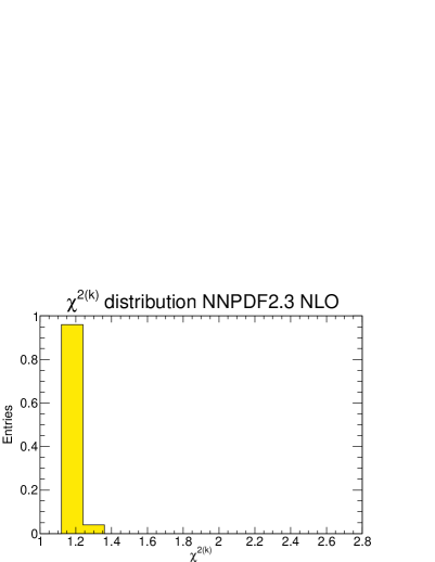
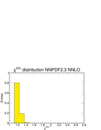
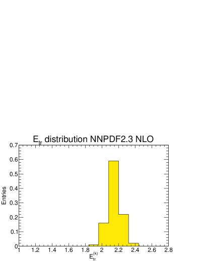
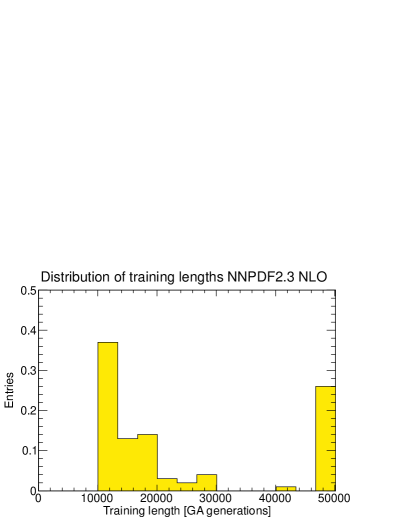
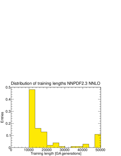
The distribution of $\chi^{2(k)}$, $E^{(k)}_{\rm tr}$, and training lengths among the $100$ NNPDF2.3 NLO and NNLO replicas are shown in Fig. 2 and Fig. 3 respectively. While most of the replicas fulfil the stopping criterion, a fraction ($\sim 20\%$) of them stops at the maximum training length $N_{\rm gen}^{\rm max}$ which has been introduced in order to avoid unacceptably long fits. As in previous PDF determinations, we have explicitly verified that if we were to discard all replicas that do not stop dynamically, PDFs change by an amount which is smaller than a typical statistical fluctuation.

Figure 2: Distribution of $\chi^{2(k)}$ (upper plots) and $E^{(k)}_{\rm tr}$ (lower plots), over the sample of $N_{\mathrm{rep}}=100$ replicas, for the NNPDF2.3 NLO (left plots) and NNLO (right plots) PDF sets.

Figure 3: Distribution of training lengths over the sample of $N_{\mathrm{r}ep}=100$ replicas for the NNPDF2.3 NLO (left plot) and NNPDF2.3 NNLO (right plot) PDF sets.

4.2 NNPDF2.3 parton distributions

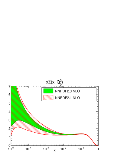
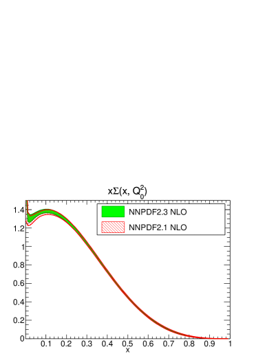
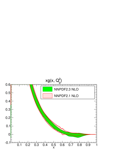
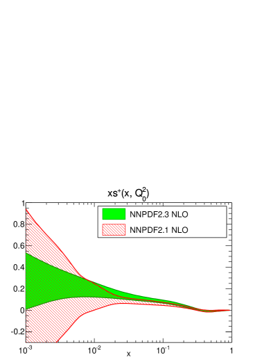
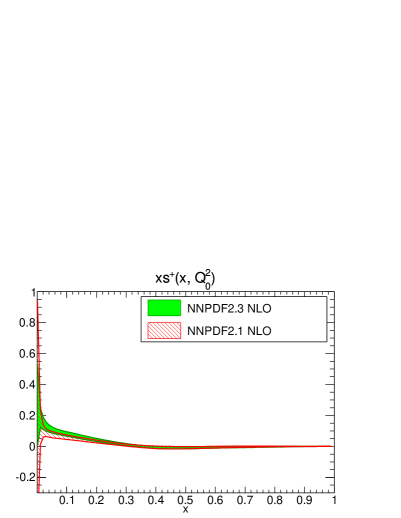
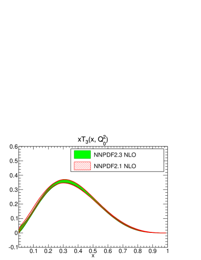
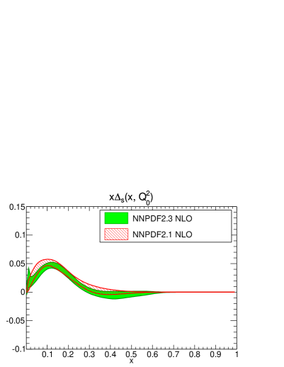
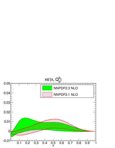
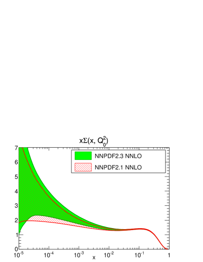
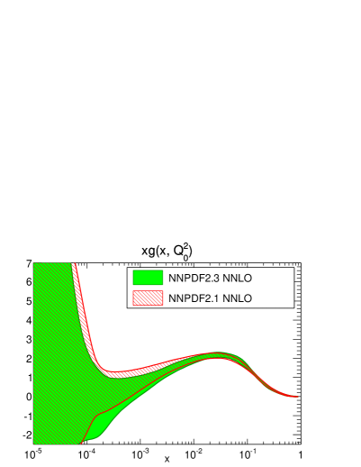
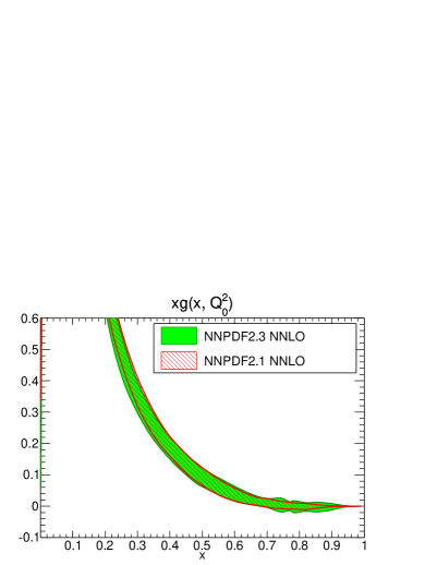
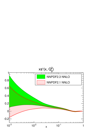
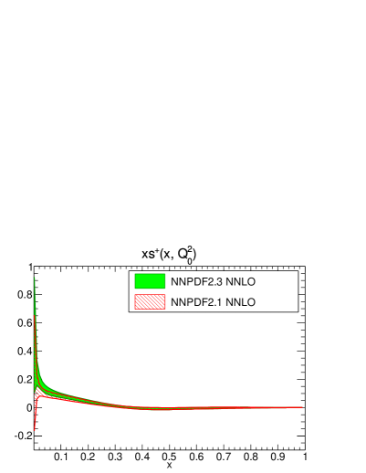
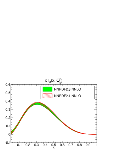
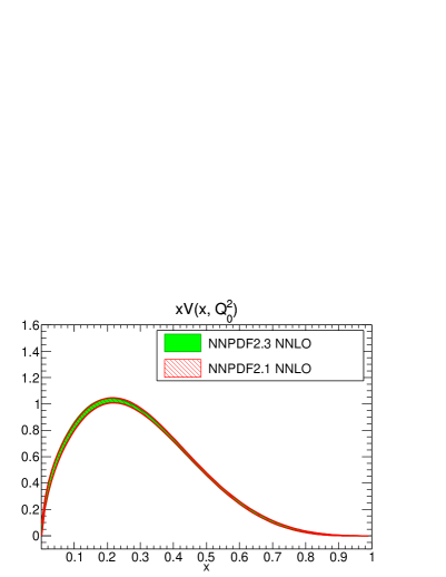
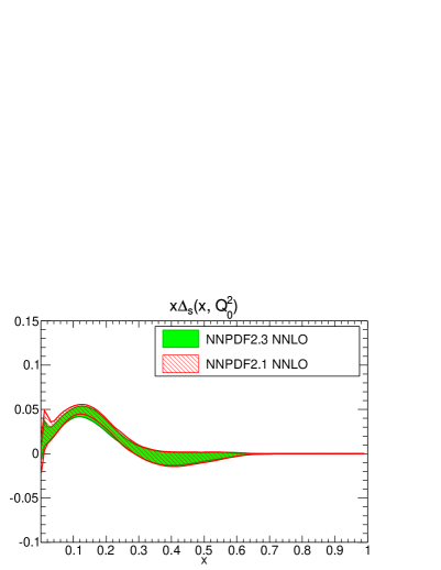
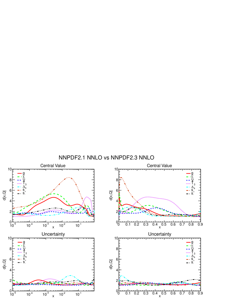
The NNPDF2.3 NLO and NNLO PDFs are shown, along with the corresponding PDFs from NNPDF2.1, in Figs. 4 & 5 (NLO) and Figs. 6 & 7 (NNLO). It is clear that all PDFs from the two sets differ by less, and usually much less, than one sigma, with differences being generally smaller at NNLO.

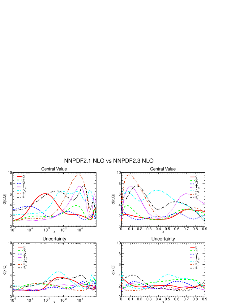
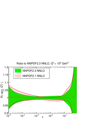
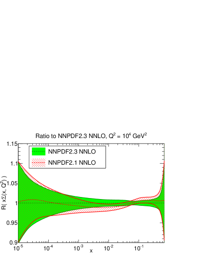
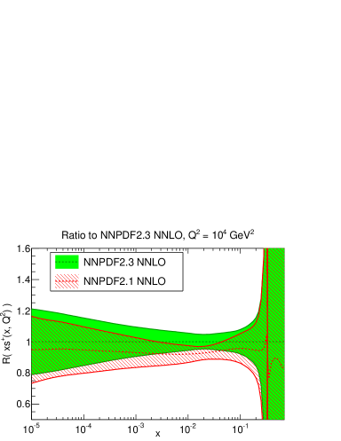
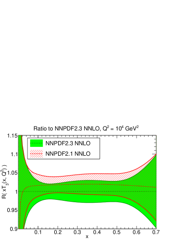
A more accurate assessment of the difference between the NNPDF2.1 and NNPDF2.3 sets can be obtained by looking at the distance between the two sets, shown in Figs. 8 & 9. The largest changes are in the gluon and in the valence flavor decomposition (i.e. in the sea asymmetry, triplet and strangeness), where we would indeed expect jet and gauge boson production to have some impact. The ratio of the NNPDF2.1 to NNPDF2.3 NNLO PDFs at $Q^{2}=10^{4}$ GeV² is shown for the gluon, singlet, triplet ans strangeness in Fig. 10. The origin of these differences is addressed in detail in Sec. 4.3

Figure 4: NLO NNPDF2.3 singlet sector PDFs at $Q^{2}=2$ GeV², compared to their NNPDF2.1 counterparts, computed using $N_{\rm rep}=100$ replicas from both sets. All error bands shown correspond to a one sigma interval.

Figure 5: Same as Fig. 4 for the nonsinglet sector NLO PDFs.

Figure 6: Same as Fig. 4 but at NNLO.

Figure 7: Same as Fig. 5 but at NNLO.

Figure 8: Distances between NNPDF2.1 and NNPDF2.3 NLO.

Figure 9: Distances between NNPDF2.1 and NNPDF2.3 NNLO.

Figure 10: The ratio of NNLO NNPDF2.1 to NNPDF2.3 gluon, singlet, (top) total strangeness and triplet (bottom) PDFs at $10^{4}$ GeV².

4.3 Detailed comparison to NNPDF2.1

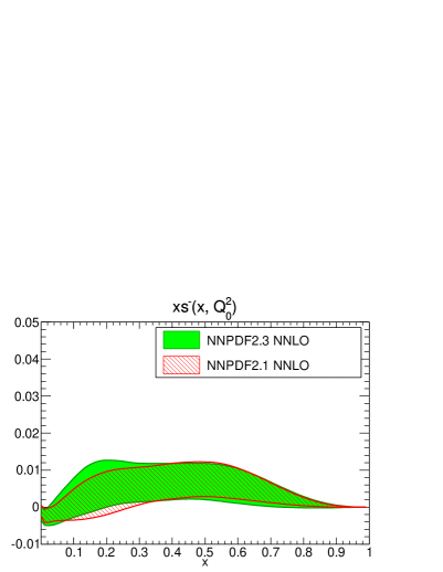
The NNPDF2.3 sets differ from the NNPDF2.1 ones not only because of the addition of LHC data, but also due to the improvements in the neural network training procedure presented in Sec. 3, and finally because of the correction of an error in Eq. (33) of Ref. [7]. This error only affects the NuTeV dimuon cross-sections, which in turn only have a significant effect on the strange distribution.

In order to isolate the effect of each of these changes, we have performed an NNPDF2.3 fit without LHC data, i.e. with the same data set as NNPDF2.1, but with the methodological improvements discussed in the previous section, supplemented by the correction of the error in the dimuon cross-section.

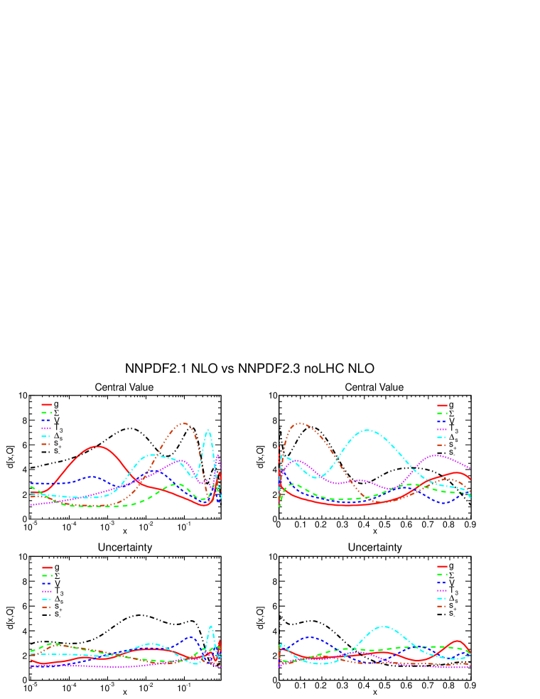
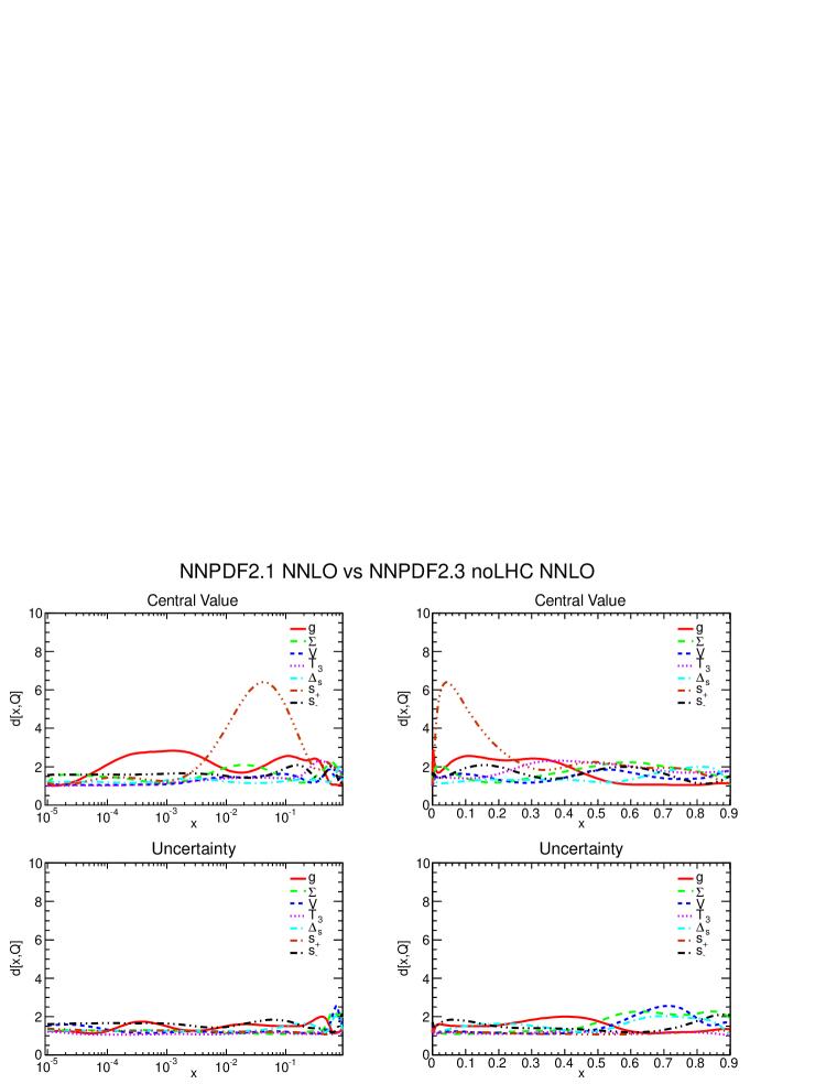
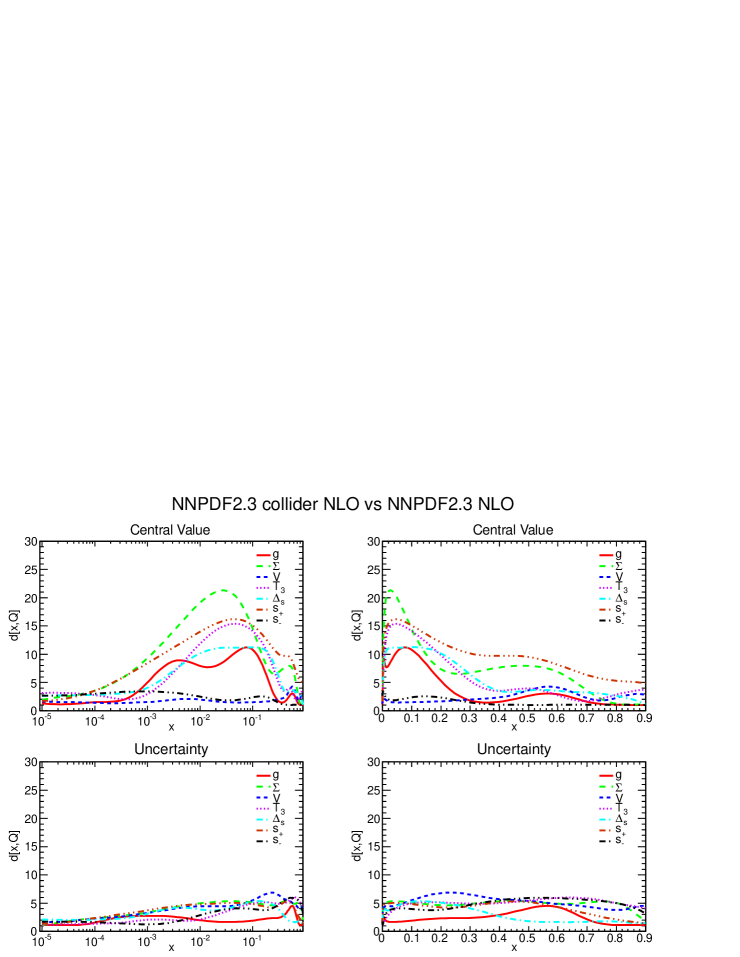
We first determine distances between NNPDF2.1 and NNPDF2.3 noLHC: this measures the effect of the various improvements, with fixed data set. The distances are shown in Fig. 11 (at NLO) and 12 (at NNLO). The largest distances are observed between the NLO strange, gluon, and sea asymmetry PDFs, for which a direct comparison between NNPDF2.1 and NNPDF2.3 noLHC is shown in Fig. 4.1.

At NNLO the distances for essentially all PDFs except total strangeness are compatible with purely statistical fluctuations ($d\sim 1$ corresponds to statistically equivalent fits). Strangeness (also shown in Fig. 4.1) changes in a statistically significant way, though at most by about half sigma, in the $10^{-2}\mathrel{\hbox to0.0pt{\lower 4.0pt\hbox{\hskip 1.0pt$\sim$}\hss}\raise 1.0pt\hbox{$<$}}x\mathrel{\hbox to0.0pt{\lower 4.0pt\hbox{\hskip 1.0pt$\sim$}\hss}\raise 1.0pt\hbox{$<$}}10^{-1}$ range. We have checked that if the error in Eq. (4) is corrected with everything else left unchanged, then the distance in strangeness is somewhat smaller, but roughly of the same order: hence the change in strangeness is mostly due to the correction of this error. It is interesting to observe that, despite the fact that the change in each individual PDF is statistically insignificant, the improvement quality of the global fit is still significant: the $\chi^{2}$ per data point decreases from $1.167$ to $1.147$, corresponding to an decrease by about $70$ units of the total $\chi^{2}$ of the fit (which corresponds to a decrease of the $\chi^{2}$ by slightly more than one sigma). Note that this decrease is not due to the NuTeV dimuon data, whose $\chi^{2}$ only decreases by a couple units, and thus it must be attributed to the improved minimization. Because at NNLO this only amounts to more stringent stopping and higher maximum number of iterations, we must conclude that the higher $\chi^{2}$ value in the NNPDF2.1 NNLO fit was due to slight underlearning.

The improvement in fit quality is even more marked at NLO, where essentially all PDFs undergo changes at the half sigma level, and the $\chi^{2}$ decreases by about 150 units (i.e. about two sigma). The fact that more significant changes are observed in PDF shapes at NLO can be understood as a consequence of having increased the number of mutations and mutants in this case.

Figure 11: Distances between NNPDF2.3 noLHC and NNPDF2.1 NLO.

Figure 12: Distances between NNPDF2.3 noLHC and NNPDF2.1 NNLO.

Figure 13: Comparison of some PDFs from the NNPDF2.1 and NNPDF2.3 noLHC sets: top: NLO small $x$ gluon (left), $\bar{d}-\bar{u}$ (right); middle: NLO $s^{-}=s-\bar{s}$ small $x$ (left), large $x$ (right) at $Q^{2}=2$ GeV²; bottom small $x$ $s^{+}=s+\bar{s}$ at NLO (left) and NNLO (right).

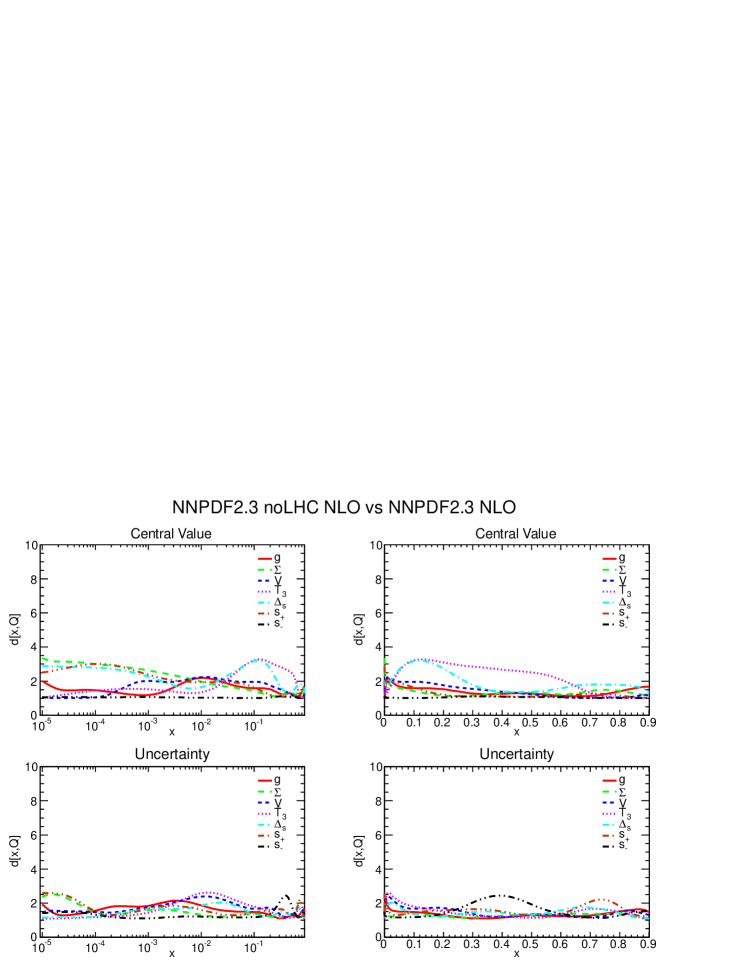
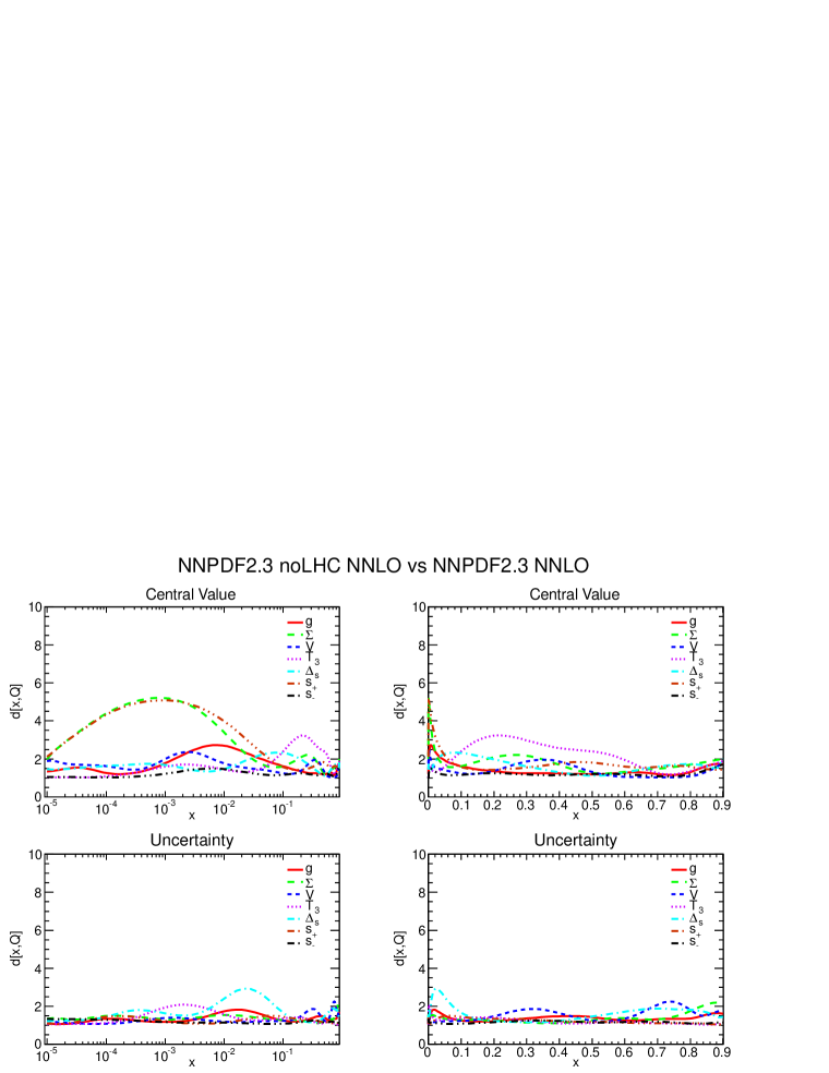
Next we compare the NNPDF2.3 noLHC and the NNPDF2.3 fits at NLO and NNLO, in order to gauge the genuine impact of LHC data. The distances between these two fits are shown in Fig. 14 and 15. The largest distances in central values are observed between the NNLO total strangeness and quark singlet at small $x$ PDFs, and to a lesser extent the gluon for all of which a direct comparison between NNPDF2.1 and NNPDF2.3 noLHC is shown in Fig. 4.1.

The impact of LHC data is clearly moderate, with no distance larger than four at NLO, which means that the fitted PDFs differ by less than half sigma. At NNLO the effect seems to be a bit larger. This confirms the consistency of the PDFs extracted from lower energy experiments with the PDFs extracted from LHC data. The description of the LHC experiments is of course better in NNPDF2.3 than in NNPDF2.3 noLHC, although the starting agreement was already very reasonable, as is clearly seen in the $\chi^{2}$ comparison shown in Tab. 4.1.

While all changes are moderate, the main effect of the LHC data is to lead to somewhat smaller gluon uncertainties, thanks to the inclusion of the ATLAS jet data, and especially a more accurate light quark flavor decomposition thanks to the LHC electroweak vector boson production data. This in turn leads to an improvement in the accuracy of standard candle cross-sections, both dependent on the gluon (top production) and the quark (gauge boson production), as we will see in Sec. 6.2.

Figure 14: Distances between NNPDF2.3 noLHC and NNPDF2.3 NLO.

Figure 15: Distances between NNPDF2.3 noLHC and NNPDF2.3 NNLO.

Figure 16: Comparison of some PDFs from the NNPDF2.3 noLHC and NNPDF2.3 NNLO sets. Top: gluon at small $x$ (left) and large $x$ (right); bottom: small $x$ total singlet (left) and total strangeness (right).

5 The LHC data

We will now address in more detail the impact of LHC data on NNPDF2.3 parton distributions. First, we extend the discussion of Sec. 4.3, where NNPDF2.3 fits with and without LHC data were compared, by comparing a fit in which LHC data are included in the full fitting data set with a fit in which the LHC data are included by reweighting a fit which does not include them: this enables us to assess more accurately both the impact and the consistency of the LHC data in the global fit. This analysis is supplemented by an explicit assessment of the quality of the fit to LHC data before and after their inclusion. We then consider a PDF determination which is based on collider data only. This enables us to discuss the consistency between collider data and the lower-energy fixed-target data, several of which are affected by nuclear corrections. The LHC data, by expanding the set of available collider data, sheds some further light on this comparison. Finally, we present a dedicated analysis of the strangeness fraction of the nucleon, and the impact of LHC data on its determination.

5.1 Impact and consistency of the LHC data in the global fit

New data can be included in an existing PDF fit either by simply redoing the fit, or by reweighting the replicas of an existing fit [6, 4]. Besides providing a strong consistency check of the fitting procedure, the inclusion of the data by reweighting allows one to test for the impact and consistency of the new data. For example, one can determine the probability distribution $P(\alpha)$ for the rescaling of uncertainties of the new data set by a factor $\alpha$: for fully consistent data the mean value of $\alpha$ should be $\langle\alpha\rangle\sim 1$. Furthermore, one may determine the effective number of replicas $N_{\rm eff}$ left after reweighting the initial set of $N_{\rm rep}$ replicas: if $N_{\rm eff}\ll N_{\rm rep}$ the new data either bring in considerable new information or they are very inconsistent with the pre-existing data, and conversely.

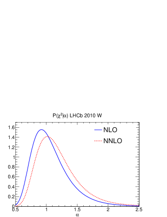
We have thus performed the reweighting of a set of $500$ NNPDF2.3 noLHC NLO or NNLO replicas with $\alpha_{s}(M_{\rm Z})=0.119$ with the various LHC data sets. The $\chi^{2}$ obtained comparing to the data predictions obtained using this reweighted set are compared in Tab. 4.1 to those of the standard NNPDF2.3 NLO and NNLO fits. The good agreement between reweighted and refitted $\chi^{2}$ values provides evidence for the consistency and efficiency of the fitting methodology. Furthermore, in Fig. 17 we show the probability distributions $P(\alpha)$ for each of the four LHC data sets added to the fit, at NLO and NNLO, and in Tab. 8 the values of $\langle\alpha\rangle$ and $N_{\rm eff}$ obtained by reweighting at NLO or NNLO first with each LHC data set individually, and then with all LHC data. The values of $P(\alpha)$ distributions generally show good consistency of the LHC data with the rest, with perhaps a marginal inconsistency for the ATLAS and CMS gauge boson production. This might suggest some tension between the flavor decomposition favoured by low energy and collider data, to which we will return in Sec. 5.2. The values of $N_{\rm eff}$ show that even though the impact of the LHC data is moderate, it is not negligible: for example, the ATLAS gauge boson production data alone effectively discard more than two thirds of the starting replicas. The impact of the LHC data is clearly seen in Tab. 4.1: the uncertainty in the prediction for gauge boson production at the LHC is roughly halved if NNPDF2.3 PDFs rather than NNPDF2.3 noLHC PDFs are used.

NNPDF2.3 noLHC reweighted with LHC data
	NLO		NNLO
	$N_{\rm eff}$	$\left\langle\alpha\right\rangle$	$N_{\rm eff}$	$\left\langle\alpha\right\rangle$
ATLAS W/Z	285	1.4	134	1.6
CMS W e asy	284	1.6	290	1.6
LHCb W	492	1.1	483	1.2
ATLAS inclusive jets	476	1.0	456	0.9
All LHC data	338	1.1	271	1.2

Table 8: The effective number of replicas $N_{\rm eff}$ and average uncertainty rescaling $\langle\alpha\rangle$ (defined in Refs. [6, 4]) obtained by reweighting a set of $N_{\rm rep}=500$ NNPDF2.3 noLHC NLO and NNLO replicas with $\alpha_{s}(M_{\rm Z})=0.119$ with each of the LHC data sets, and with all of them.

Figure 17: The $P\left(\alpha\right)$ distributions for each of the LHC experiments included in NNPDF2.3: the ATLAS 2010 jets, the ATLAS 2010 W,Z data, the CMS 2011 W electron asymmetry and the LHCb 2010 W data, all determined using either NLO or NNLO theory, with $\alpha_{s}(M_{\rm Z})=0.119$. The mean values of $\alpha$ computed from each of these distributions are given in Tab. 8.

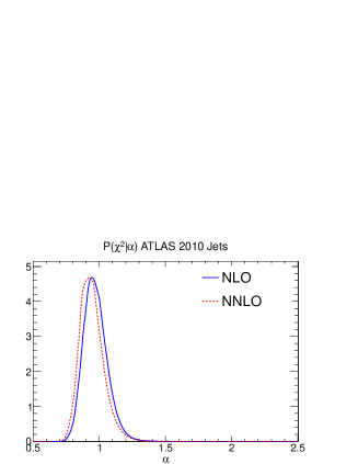
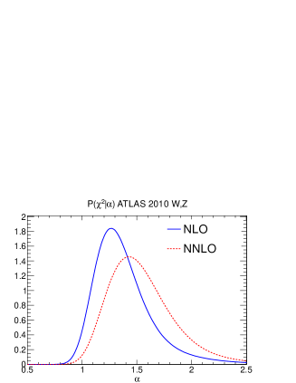
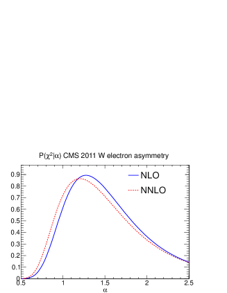
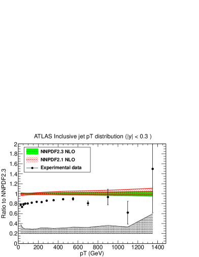
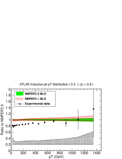
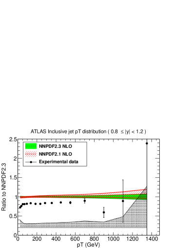
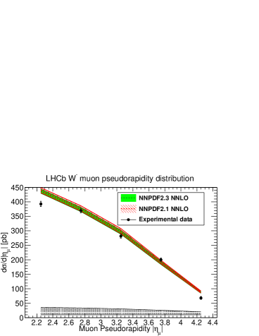
The impact of the LHC data can also be seen by comparing the predictions for the fitted observables before and after their inclusion in the fit: as shown in Sec. 4.3 the $\chi^{2}$ values of Tab. 4.1 already show that the fit quality is acceptable before including the LHC data, and quite good after including them. This is also seen from a data-theory comparison: the predictions from the NNPDF2.1 and NNPDF2.3 $\alpha_{s}(M_{\rm Z})=0.119$ sets for the various LHC observables are compared to the data in Fig. 18 (ATLAS jets), Fig. 19 (ATLAS and CMS W,Z production) and Fig. 20 (LHCb W production). For the LHC electroweak data we show the predictions from the NNLO PDF sets, while for the ATLAS inclusive jets we show the corresponding NLO predictions: for jets the results are normalized to the NNPDF2.3 prediction. Note that much of the uncertainty in the jet data is the totally correlated normalization uncertainty, which can shift the entire data set up or down, so that inspection of the plot can be somewhat misleading and the $\chi^{2}$ values of Tab. 4.1 should be checked in order to assess fit quality.

Figure 18: Comparison of the ATLAS inclusive jet data with predictions from NNPDF2.1 and NNPDF2.3 NLO PDFs with $\alpha_{s}(M_{\rm Z})=0.119$. We show the ratio of data over theory, normalized to NNPDF2.3, divided into rapidity bins. The experimental error bars are statistical, while the (correlated) systematic uncertainty, including normalization errors, is shown as a band in the bottom of each plot.

Figure 19: Same as Fig. 18, but for ATLAS and CMS gauge boson production data, now using NNLO PDFs.

Figure 20: Same as Fig. 18, but for LHCb electroweak gauge boson production data, now using NNLO PDFs.

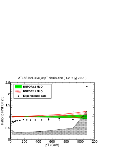
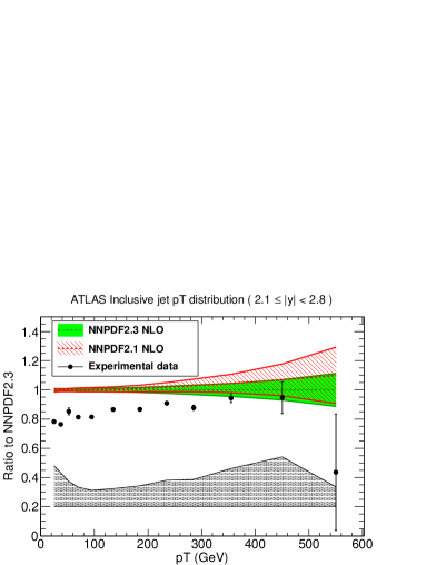
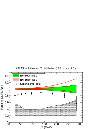
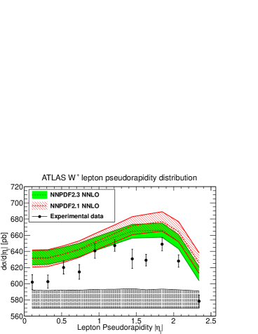
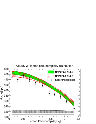
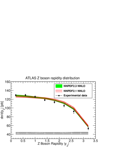
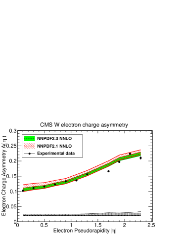
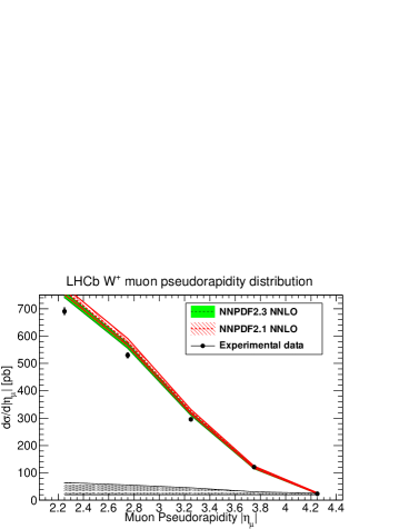
5.2 Consistency of LHC data with low-energy data

It has been previously observed [6, 101, 102] that there seems to be some tension between the flavor decomposition favoured by low energy data, and that obtained from Tevatron W production data. The LHC data will eventually solve any such discrepancy: in fact, they already shed some light on this issue. To investigate this, as already mentioned, we have constructed sets of NLO and NNLO NNPDF2.3 collider PDFs. The NNPDF2.3 collider PDFs are based on a data set which includes only the HERA-I inclusive data, the ZEUS HERA-II data and the H1 and ZEUS $F_{2}^{c}$ charm structure function data, the W and Z production data from the Tevatron and the LHC, the CDF and D0 Run II inclusive jet production data and the ATLAS inclusive jet data. This reduces the size of the data set from about 3500 to about 1200 data points (see Tab. 2).

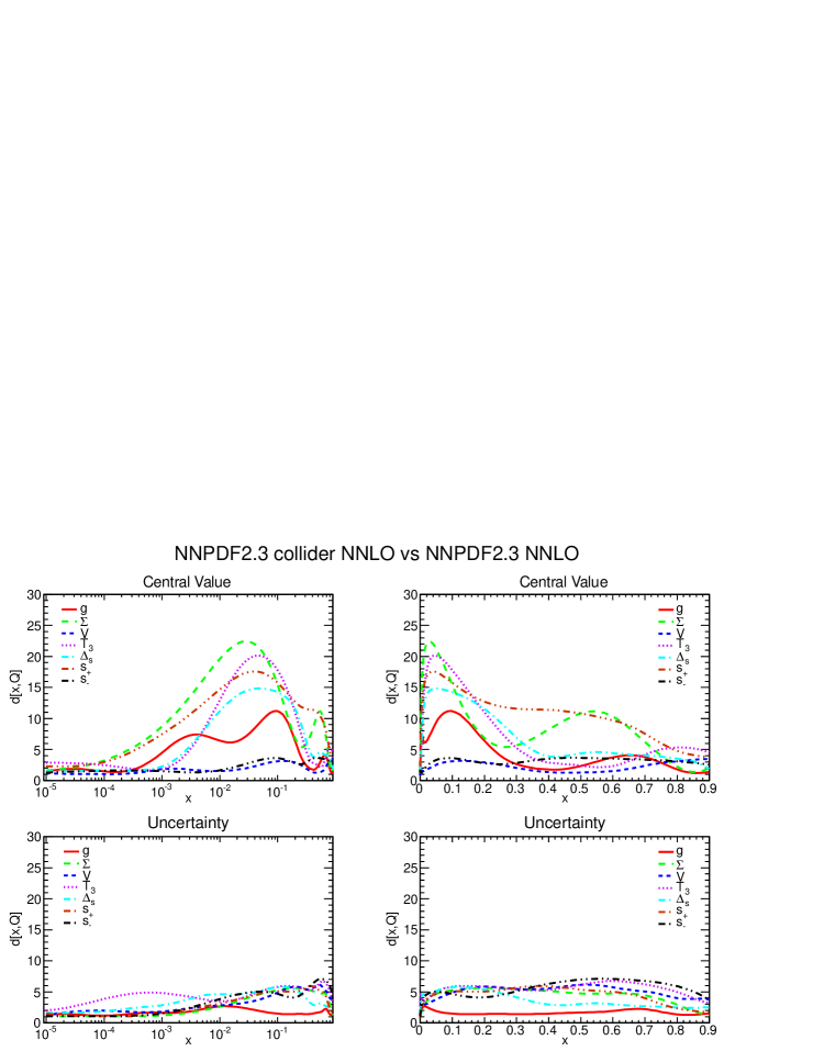
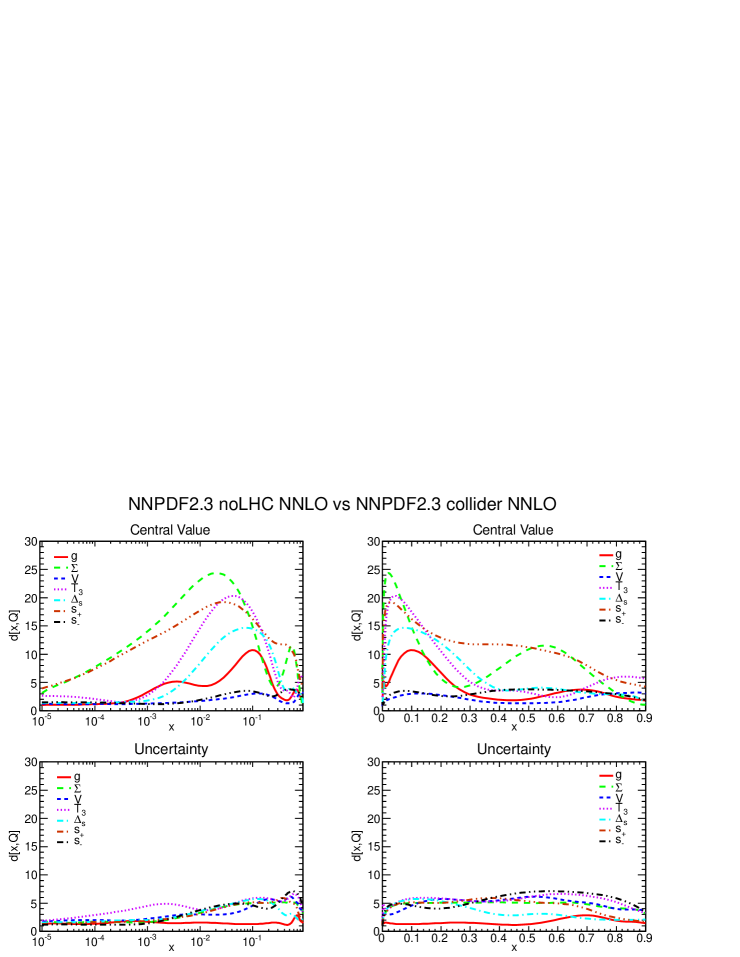
The distance between PDFs in the NNPDF2.3 collider and NNPDF2.3 default data sets at NLO and NNLO with $\alpha_{s}(M_{\rm Z})=0.119$ are shown in Figs. 21–22 respectively, while the distances between NNPDF2.3 collider and NNPDF2.3 noLHC PDFs are in Figs. 23–24. We note that almost all PDFs change at the one or two sigma level, both at NLO and NNLO. There are no significant differences between the pattern of distances observed at NLO or NNLO, or when comparing to the standard or noLHC sets. This in particular suggests that the tension between collider data and low energy data, if it exists, is only mild: indeed, if the low energy data were inconsistent with collider data, distances should be significantly smaller when comparing to the noLHC set than to the default set, because the former has much fewer collider data.

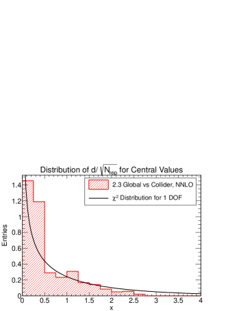
To investigate this in more detail, we have sampled the distances shown in Figs. 21–24 for each PDF at 100 points in $x$, 50 equally spaced on a log scale from $x=10^{-4}$ to $10^{-1}$, and 50 more on a linear scale from $0.1$ to $0.9$. For each comparison, we have then produced a histogram of the distribution of distances. The distance is defined for each $x$ value as a sum over replicas of normalized square differences of predictions obtained from a gaussian distribution, and thus it should follow, for each point and PDF, a $\chi^{2}$ distribution with one degree of freedom. The combined histogram still follows the same distribution if correlations are uniform. Indeed only if there is a large number of points that are correlated to one particular point will the histogram be distorted. We have verified that this is not the case by checking that the histograms do not change when redone with a decreasing number of points, which completely modifies the pattern of correlations.

The normalized histograms are compared to this $\chi^{2}$ distribution in Fig. 25: no significant difference is apparent between the four histograms, which are all well consistent with the theoretical distribution. This suggests that the differences between PDFs in the collider only and global fits are consistent with a purely statistical distribution, based on the given PDF uncertainties. This means that, the different behaviour of 2.3 and 2.3 collider PDFs which is seen in Fig. 4.1 (e.g. for the triplet at small $x$) is compatible with a statistical fluctuation.

Figure 21: Distances between PDFs from the NNPDF2.3 collider and NNPDF2.3 NLO sets.

Figure 22: Distances between PDFs from the NNPDF2.3 collider and NNPDF2.3 NNLO sets.

Figure 23: Distances between PDFs from the NNPDF2.3 collider and NNPDF2.3 noLHC NLO sets.

Figure 24: Distances between PDFs from the NNPDF2.3 collider and NNPDF2.3 noLHC NLO sets.

Based on these conclusions, one might be tempted to recommend usage of the collider PDFs, in that they are free from nuclear corrections and much less sensitive to possible higher twist corrections, while retaining the abundant, statistically accurate, and theoretically very reliable deep-inelastic data from the HERA experiments. This option however turns out to be not viable at present, because the collider PDFs still have rather large statistical uncertainties. This is apparent from Tab. 4.1, where it is seen that the uncertainties of all the observables measured by fixed-target experiments become unacceptably large when the NNPDF2.3 collider fit is used. It is also visible in Fig. 4.1, where we compare the singlet, gluon triplet and sea asymmetry in the collider and default NNLO fits. This means that a collider-only fit is presently not viable, though this situation may change for future collider PDFs, which will include both the final, yet unpublisjed, HERA-II combined deep-inelastic data, as well as future LHC data.

Figure 25: Distribution of distances between PDFs from the NNPDF2.3 collider and NNPDF2.3 NLO and NNLO sets (top) and between PDFs from the NNPDF2.3 collider and NNPDF2.3 noLHC NLO and NNLO sets (bottom). The $\chi^{2}$ distribution with one degree of freedom is also shown.

Figure 26: Comparison of the singlet, gluon (top), triplet $u+\bar{u}-d-\bar{d}$ and sea asymmetry $\bar{d}-\bar{u}$ at $Q^{2}=2$ GeV² from the NNLO NNPDF2.3 collider and NNPDF2.3 sets with $\alpha_{s}(M_{\rm Z})=0.119$.

5.3 The strangeness fraction of the proton

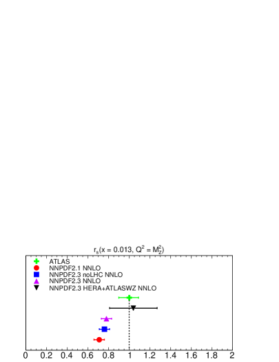
The ATLAS collaboration has recently [24] presented evidence that the strange quark distribution at low $Q^{2}$ and $x$ is rather larger than hitherto thought, so that, for the specific kinematics probed by ATLAS ($Q^{2}=1.9$ GeV², $x=0.023$) the quark sea is essentially symmetric. This result, if correct with the stated uncertainty, disagrees at the two sigma level with the result obtained using the NNPDF2.1 set. The ATLAS analysis is based on combining ATLAS and HERA data, i.e. on a subset of the data used to construct the NNPDF2.3 collider fit discussed in Sec. 5.2: as we have seen there, PDFs based on collider data only have very large uncertainties, so such a discrepancy seems surprising. This is especially so given the fact that the strangeness distributions in the NNPDF2.1 and NNPDF2.3 sets (the latter including ATLAS data) always agree at the one sigma level, as can be seen from Fig. 10.

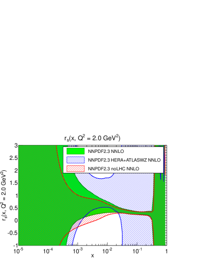
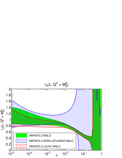
In order to check the ATLAS result, we have produced a version of the NNPDF2.3 fit based on exactly the same data set, namely only the combined HERA-I data (HERAI-AV in Tab. 2 of [7]) and the ATLAS gauge production data (ATLAS W^± and ATLAS Z in Tab. 1), with a single value of $\alpha_{s}(M_{\rm Z})=0.119$. This PDF set will be denoted in the following as NNPDF2.3 HERA+ATLASWZ. Following Ref. [24], we define the $x$-dependent strangeness fraction

$$r_{s}(x,Q^{2})={{s(x,Q^{2})+\bar{s}(x,Q^{2})}\over{2\bar{d}(x,Q^{2})}}\,.$$ (17)

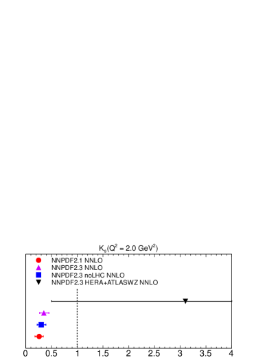
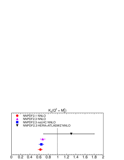
A perhaps more significant measure of the strangeness content is the strangeness momentum fraction normalized to the light sea momentum fraction [103, 104, 15, 105]

$$K_{s}(Q^{2})={{\int_{0}^{1}dxx\left(s(x,Q^{2})+\bar{s}(x,Q^{2})\right)}\over{\int_{0}^{1}dxx\left(\bar{u}(x,Q^{2})+\bar{d}(x,Q^{2})\right)}}\,,$$ (18)

traditionally [106] taken to be $K_{s}\approx 0.5$ at scales of a few GeV.

The strangeness fraction $r_{s}(x,Q^{2})$ Eq. (17) was determined in Ref. [24] at the two points in the $(x,Q^{2})$ plane $(x,Q^{2})=(0.023,1.9~{}{\rm GeV}^{2})$ and $(x,Q^{2})=(0.013,M_{\rm Z}^{2})$. In Fig. 27 we show $r_{s}(x,Q^{2})$ computed as a function of $x$ for the relevant scales, as obtained using the NNPDF2.3 noLHC, NNPDF2.3 and NNPDF2.3 HERA+ATLASWZ NNLO PDF sets with $\alpha_{s}(M_{\rm Z})=0.119$. It is clear that the strangeness fraction computed with NNPDF2.3 PDFs, especially in the range $10^{-3}\mathrel{\hbox to0.0pt{\lower 4.0pt\hbox{\hskip 1.0pt$\sim$}\hss}\raise 1.0pt\hbox{$<$}}x\mathrel{\hbox to0.0pt{\lower 4.0pt\hbox{\hskip 1.0pt$\sim$}\hss}\raise 1.0pt\hbox{$<$}}10^{-1}$, is somewhat larger than the NNPDF2.3 noLHC one, though they are fully consistent at the one sigma level for all values of $x$. This means that even though the ATLAS data do push the strangeness fraction towards slightly higher values, the effect is of marginal statistical significance. If the comparison is made with the NNPDF2.3 HERA+ATLASWZ fits, then uncertainties are so large that results become completely compatible.

Figure 27: The strangeness fraction $r_{s}(x,Q^{2})$ Eq. (17) computed as a function of $x$ for $Q^{2}=2$ GeV² (left) and $Q^{2}=M_{\rm Z}^{2}$ GeV² (right) from NNPDF2.3 noLHC, NNPDF2.3 and NNPDF2.3 HERA+ATLASWZ NNLO PDFs with $\alpha_{s}(M_{\rm Z})=0.119$. All error bands are one sigma.

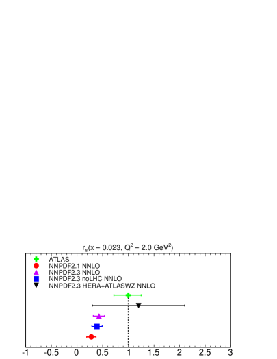
The values of the strangeness fraction at the specific values of $(x,Q^{2})$, together with the strangeness momentum fraction Eq. (18) are given in Tab. 9, and represented graphically in Fig. 28. The values of the strangeness fraction from Ref. [24] are also shown (note that in the latter case the low-scale value is given at $Q^{2}=1.9$ GeV², while for NNPDF it is at $Q^{2}=2$ GeV².)

The conclusions are the same as were drawn from Fig. 27: the ATLAS data favour a somewhat larger central value of the strangeness fraction, which remains however compatible at the one sigma level with the value obtained without LHC data (NNPDF2.3 noLHC), and also consistent with the previous, slightly less accurate NNPDF2.1 value. However, it seems that the “standard” belief that the strange momentum fraction is of order $K_{s}\approx{{1}\over{2}}$ is still essentially correct.

If one then attempts a determination based on HERA and ATLAS data only, then uncertainties are so large that no conclusion can be drawn: the NNPDF2.3 HERA+ATLASWZ result for $r_{s}$ has an uncertainty which is three to four times bigger than that of the ATLAS result of Ref. [24], and indeed for this PDF set $K_{S}$ is essentially undetermined. Because the ATLAS analysis is based on the same data, and only differs from our analysis in the fitting methodology (in particular, the use of a rather simple functional form for PDFs), it appears likely that the uncertainties in the results of Ref. [24] are significantly underestimated.

PDF Set	$r_{s}(0.023,2~{}\mathrm{GeV}^{2})$	$r_{s}(0.013,M_{\rm Z}^{2})$
NNPDF2.1	$0.28\pm 0.09$	$0.71\pm 0.05$
NNPDF2.3 noLHC	$0.39\pm 0.10$	$0.76\pm 0.05$
NNPDF2.3	$0.43\pm 0.11$	$0.78\pm 0.05$
NNPDF2.3 HERA+ATLASWZ	$1.2\pm 0.9$	$1.04\pm 0.23$
ATLAS (Ref. [24])	$1.00\,{}^{+0.25}_{-0.28}$	$1.00\,{}^{+0.09}_{-0.10}$

PDF Set	$K_{s}(2~{}\mathrm{GeV}^{2})$	$K_{s}(M_{\rm Z}^{2})$
NNPDF2.1	$0.26^{+0.08}_{-0.08}$	$0.63^{+0.04}_{-0.05}$
NNPDF2.3 noLHC	$0.30^{+0.09}_{-0.08}$	$0.65^{+0.05}_{-0.05}$
NNPDF2.3	$0.35^{+0.10}_{-0.08}$	$0.68^{+0.05}_{-0.05}$
NNPDF2.3 HERA+ATLASWZ	$3.1^{+0.9}_{-2.6}$	$1.3^{+0.5}_{-0.6}$

Table 9: The strangeness fraction Eq. (17) (top table) and strangeness momentum fraction Eq. (18) (bottom table) determined using the NNPDF2.1, NNPDF2.3 noLHC, NNPDF2.3 and NNPDF2.3 HERA+ATLASWZ NNLO PDF sets with $\alpha_{s}(M_{\rm Z})=0.119$. The values of Ref. [24] are also shown (note that for ATLAS the low-scale value is given at $Q^{2}=1.9$ GeV²). The PDF uncertainties in the strangeness fraction Eq. (17) are one sigma errors while in the strangeness momentum fraction Eq. (18) they are 68% confidence levels.

Figure 28: Graphical representation of the results of Tab. 9. Note the different scale on the $x$ axis.

6 Phenomenology

We discuss now some phenomenological implications of the NNPDF2.3 parton set. After briefly discussing NNPDF2.3 parton luminosities, we use them to compute several LHC reference “standard candle” cross-sections.

6.1 Parton luminosities

At a hadron collider, all factorized observables depend on parton distributions through a parton luminosity, which, following Ref. [107], we define as

$$\Phi_{ij}\left(M_{X}^{2}\right)={{1}\over{s}}\int_{\tau}^{1}{{dx_{1}}\over{x_{1}}}f_{i}\left(x_{1},M_{X}^{2}\right)f_{j}\left(\tau/x_{1},M_{X}^{2}\right)\ ,$$ (19)

where $f_{i}(x,M^{2})$ is a PDF and $\tau\equiv M_{X}^{2}/s$. The parton luminosity thus contains all the information on the dependence of hadronic cross-sections on PDFs.

Figure 29: Comparison of the parton luminosities for LHC at 8 TeV, computed using the NNPDF2.1 and NNPDF2.3 NNLO PDFs, using $N_{\rm rep}=100$ replicas from both sets. From left to right we show $\Phi_{gg}$, $\Phi_{qg}$, (top) $\Phi_{q\bar{q}}$, $\Phi_{c\bar{c}}$, (middle) $\Phi_{b\bar{b}}$, $\Phi_{bg}$ (bottom). All luminosities are plotted as ratios to the NNPDF2.3 NNLO central value. All uncertainties shown are one sigma.

Parton luminosities computed for LHC 8 TeV using NNPDF2.1 and NNPDF2.3 PDFs at NNLO with $\alpha_{s}(M_{\rm Z})=0.119$ are compared in Fig. 4.1. The NLO luminosities are quite similar. All the luminosities are very compatible at the one sigma level. In particular, the gluon-gluon luminosity, which is relevant for Higgs production at the LHC, is quite stable in the region which corresponds to Standard Model Higgs production. The heavy quark PDFs follow the behaviour of the gluon, from which they are generated dynamically via perturbative evolution. Note that the masses of the heavy quarks $m_{\rm c}$ and $m_{\rm b}$ are the same in the NLO and NNLO analyses.

In going from NNPDF2.1 to NNPDF2.3, the uncertainty on the gluon-gluon luminosity is reduced somewhat for larger final state invariant masses, while the $q\bar{q}$ luminosity is somewhat smaller in the same region. As discussed in Sec. 4.3, the former effect is due both to the improved genetic algorithm minimization and the impact of the ATLAS inclusive jet data, while the latter is due to the impact of the LHC electroweak vector boson production data.

	$\sigma({\rm W}^{+})$		$\sigma({\rm W}^{-})$		$\sigma({\rm Z}^{0})$
	NLO	NNLO	NLO	NNLO	NLO	NNLO
NNPDF2.1	5.891 $\pm$ 0.133	6.198 $\pm$ 0.098	4.015 $\pm$ 0.091	4.213 $\pm$ 0.068	0.928 $\pm$ 0.018	0.972 $\pm$ 0.013
NNPDF2.3	5.854 $\pm$ 0.076	6.122 $\pm$ 0.078	4.057 $\pm$ 0.053	4.202 $\pm$ 0.059	0.931 $\pm$ 0.011	0.968 $\pm$ 0.012
NNPDF2.3 noLHC	5.886 $\pm$ 0.082	6.198 $\pm$ 0.109	4.039 $\pm$ 0.066	4.218 $\pm$ 0.072	0.931 $\pm$ 0.012	0.974 $\pm$ 0.015
NNPDF2.3 collider	5.845 $\pm$ 0.104	6.127 $\pm$ 0.107	4.071 $\pm$ 0.074	4.234 $\pm$ 0.068	0.953 $\pm$ 0.016	1.000 $\pm$ 0.020

	$\sigma({\rm W})/\sigma({\rm Z}^{0})$		$\sigma({\rm W}^{+})/\sigma({\rm W}^{-})$
	NLO	NNLO	NLO	NNLO
NNPDF2.1	10.678 $\pm$ 0.031	10.707 $\pm$ 0.034	1.467 $\pm$ 0.018	1.471 $\pm$ 0.021
NNPDF2.3	10.650 $\pm$ 0.022	10.669 $\pm$ 0.034	1.443 $\pm$ 0.009	1.457 $\pm$ 0.013
NNPDF2.3 noLHC	10.662 $\pm$ 0.025	10.692 $\pm$ 0.026	1.457 $\pm$ 0.022	1.470 $\pm$ 0.020
NNPDF2.3 collider	10.403 $\pm$ 0.131	10.359 $\pm$ 0.124	1.436 $\pm$ 0.014	1.447 $\pm$ 0.015

Table 10: Total cross-sections for W and Z production at the LHC at $\sqrt{s}=7$ TeV. All uncertainties shown are one sigma (in nb). Branching ratios are included in the cross-section.

	$\sigma({\rm t\bar{t}})$		$\sigma({\rm H})$
	NLO	NNLO	NLO	NNLO
NNPDF2.1	160.1 $\pm$ 5.4	158.6 $\pm$ 4.4	11.40 $\pm$ 0.18	15.22 $\pm$ 0.22
NNPDF2.3	158.3 $\pm$ 4.0	157.1 $\pm$ 4.2	11.46 $\pm$ 0.13	15.31 $\pm$ 0.20
NNPDF2.3noLHC	158.4 $\pm$ 4.3	157.1 $\pm$ 4.7	11.48 $\pm$ 0.14	15.30 $\pm$ 0.17
NNPDF2.3–collider	151.2 $\pm$ 6.1	150.0 $\pm$ 5.3	10.80 $\pm$ 0.25	14.44 $\pm$ 0.27

Table 11: Total cross-sections for top quark pair production and Higgs production in gluon fusion at the LHC at $\sqrt{s}=7$ TeV (in pb). All uncertainties shown are one sigma

6.2 Total cross-sections

We present now results for several benchmark total cross-sections at the LHC at NLO and NNLO using NNPDF2.3 PDFs as well as NNPDF2.1 PDFs for comparison, with $\alpha_{s}(M_{\rm Z})=0.119$ at the LHC, and $\sqrt{s}=7$ TeV and $\sqrt{s}=8$ TeV. We determine the following observables:

• electroweak gauge boson production total cross-sections and ${\rm W}^{+}/{\rm W}^{-}$ and W/Z cross-section ratios, using the Vrap code [108] with scale $Q^{2}=M_{\rm V}^{2}$;

• top pair production total cross-section, using the top++ code [109] with $Q^{2}=m_{\rm t}^{2}$; at NNLO the approximate cross-sections of Ref. [110] are used; the settings are the default ones of Ref. [23], and are the same at NLO and NNLO; in particular the top quark mass is taken to be $m_{\rm t}=173.3$ GeV; use the same settings for the calculations with NLO and NNLO PDFs.

• Standard Model Higgs boson production cross-sections with $m_{\rm H}=125$ GeV in the gluon fusion using the iHixs code [111] with $Q=m_{\rm H}$.

All uncertainties shown are PDF uncertainties only: in particular they do not include the uncertainty due to the variation of $\alpha_{s}$, nor theoretical uncertainties, in particular the uncertainty due to missing higher orders, usually estimated by varying renormalization and factorization scales.

Results are collected in Tabs. 11 & 11 ($\sqrt{s}=7$ TeV) and in Tabs. 13 & 13 ($\sqrt{s}=8$ TeV), and represented graphically in Fig. 4.1. For all observables it is clear that even though everything is consistent within uncertainties, the accuracy increases when going from NNPDF2.1 to NNPDF2.3. Comparison with results obtained using the NNPDF2.3 noLHC sets shows that improvement is partly due to the improved methodology, but the LHC data have a visible impact both on the central value and uncertainty. Results obtained using the collider only set are not yet competitive, even for these very inclusive observables, except for quantities such as the ${\rm W}^{+}/{\rm W}^{-}$ ratio which are determined primarily by the collider data.

	$\sigma({\rm W}^{+})$		$\sigma({\rm W}^{-})$		$\sigma({\rm Z}^{0})$
	NLO	NNLO	NLO	NNLO	NLO	NNLO
NNPDF2.1	6.759 $\pm$ 0.152	7.116 $\pm$ 0.112	4.683 $\pm$ 0.103	4.918 $\pm$ 0.078	1.078 $\pm$ 0.021	1.131 $\pm$ 0.015
NNPDF2.3	6.718 $\pm$ 0.087	7.033 $\pm$ 0.090	4.731 $\pm$ 0.061	4.907 $\pm$ 0.067	1.082 $\pm$ 0.013	1.127 $\pm$ 0.013
NNPDF2.3 noLHC	6.756 $\pm$ 0.090	7.120 $\pm$ 0.124	4.715 $\pm$ 0.074	4.927 $\pm$ 0.082	1.083 $\pm$ 0.013	1.134 $\pm$ 0.017
NNPDF2.3 collider	6.734 $\pm$ 0.110	7.066 $\pm$ 0.117	4.760 $\pm$ 0.080	4.957 $\pm$ 0.076	1.111 $\pm$ 0.019	1.168 $\pm$ 0.023

	$\sigma({\rm W})/\sigma({\rm Z}^{0})$		$\sigma({\rm W}^{+})/\sigma({\rm W}^{-})$
	NLO	NNLO	NLO	NNLO
NNPDF2.1	10.611 $\pm$ 0.033	10.639 $\pm$ 0.035	1.443 $\pm$ 0.017	1.447 $\pm$ 0.019
NNPDF2.3	10.580 $\pm$ 0.023	10.598 $\pm$ 0.035	1.420 $\pm$ 0.008	1.433 $\pm$ 0.012
NNPDF2.3 noLHC	10.591 $\pm$ 0.026	10.622 $\pm$ 0.028	1.433 $\pm$ 0.019	1.445 $\pm$ 0.018
NNPDF2.3 collider	10.347 $\pm$ 0.128	10.299 $\pm$ 0.124	1.415 $\pm$ 0.014	1.425 $\pm$ 0.013

Table 12: Same as Tab. 11, but for $\sqrt{s}=8$ TeV.

	$\sigma({\rm t\bar{t}})$		$\sigma({\rm H})$
	NLO	NNLO	NLO	NNLO
NNPDF2.1	229.5 $\pm$ 6.9	226.8 $\pm$ 5.8	14.52 $\pm$ 0.21	19.42 $\pm$ 0.26
NNPDF2.3	227.3 $\pm$ 5.1	225.1 $\pm$ 5.5	14.61 $\pm$ 0.16	19.54 $\pm$ 0.25
NNPDF2.3noLHC	227.5 $\pm$ 5.6	225.1 $\pm$ 6.0	14.65 $\pm$ 0.17	19.53 $\pm$ 0.21
NNPDF2.3–collider	216.8 $\pm$ 8.1	214.6 $\pm$ 7.0	13.81 $\pm$ 0.30	18.48 $\pm$ 0.32

Table 13: Same as Tab. 11, but for $\sqrt{s}=8$ TeV.

Figure 30: Graphical representation of the results of Tabs. 11–13

7 Conclusions

The NNPDF2.3 PDF set is the first global PDF set to include systematically all relevant LHC data, and it is thus arguably the most accurate PDF set currently available. LHC data are likely to play an increasing role in future refinements of PDF sets. In particular, the internal inconsistencies which were noticed long ago in fixed target DIS data [10], and the tensions between fixed target and collider data, some of which have been discussed here in Sec. 5, suggest that a reliable PDF determination should avoid low energy data and data obtained using nuclear targets, and should thus be based only on lepton-hadron or hadron-hadron collider data. Current collider data are not yet sufficient to give a competitive PDF determination by themselves (see Sec. 5). However this situation is likely to evolve very rapidly thanks to the excellent performance of the LHC and its experiments, not only as the data on the usual inclusive processes become more precise, but also through the incorporation of new processes, such as W boson production in association with charm quarks for strangeness determination [62, 112]. Cleaner data are in turn likely to stimulate further improvements in the computational and statistical methodologies used for their analysis, and in the theoretical framework used to describe them.

All the NNPDF2.3 PDF sets that have been discussed in this work are available from the NNPDF web site,

http://nnpdf.hepforge.org/ 

and through the LHAPDF interface [113]. On the NNPDF web site a Mathematica interface is also available, as well as a more complete selection of PDF plots.

Specifically, the new PDF sets that have been produced in the present analysis and are available in LHAPDF are the following:

• NNPDF2.3 NLO and NNLO sets of $N_{\rm rep}=100$ replicas, provided for all values of $\alpha_{s}$ from 0.114 to 0.124 varied in steps of $\delta\alpha_{s}=0.001$

NNPDF23_nlo_as_0114.LHgrid, $\ldots$, NNPDF23_nlo_as_0124.LHgrid; NNPDF23_nnlo_as_0114.LHgrid, $\ldots$, NNPDF23_nnlo_as_0124.LHgrid;

NNPDF2.3 NLO and NNLO PDF sets based on reduced data sets, provided for all values of $\alpha_{s}$ from 0.116 to 0.120 in steps of $0.001$: NNPDF23_nlo_noLHC_as_0116.LHgrid, $\ldots$, NNPDF23_nlo_noLHC_as_0120.LHgrid; NNPDF23_nnlo_noLHC_as_0116.LHgrid, $\ldots$, NNPDF23_nnlo_noLHC_as_0120.LHgrid; NNPDF23_nlo_collider_as_0116.LHgrid, $\ldots$, NNPDF23_nlo_collider_as_0120.LHgrid; NNPDF23_nnlo_collider_as_0116.LHgrid, $\ldots$, NNPDF23_nnlo_collider_as_0120.LHgrid;

NNPDF2.3 NLO and NNLO PDF sets in the $n_{f}=4$ and $n_{f}=5$ schemes (number of active flavors only increases up to the given value), provided for all values of $\alpha_{s}$ from 0.116 to 0.120 in steps of $0.001$: NNPDF23_nlo_FFN_NF4_as_0116.LHgrid, $\ldots$, NNPDF23_nlo_FFN_NF4_as_0120.LHgrid; NNPDF23_nnlo_FFN_NF4_as_0116.LHgrid, $\ldots$, NNPDF23_nnlo_FFN_NF4_as_0120.LHgrid; NNPDF23_nlo_FFN_NF5_as_0116.LHgrid, $\ldots$, NNPDF23_nlo_FFN_NF5_as_0120.LHgrid; NNPDF23_nnlo_FFN_NF5_as_0116.LHgrid, $\ldots$, NNPDF23_nnlo_FFN_NF5_as_0120.LHgrid;

 

Acknowledgments We are grateful to Tancredi Carli, Eric Feng, Paolo Francavilla, Pavel Starovoitov and Mark Sutton for discussions about the ATLAS jet data and the APPLgrid interface. We are grateful to Jeff Berryhill, Amanda Cooper-Sarkar, Uta Klein, Ronan McNulty, Michele Pioppi, Voica Radescu, Tara Shears and Pin Tang for discussions on the ATLAS, CMS and LHCb electroweak measurements, and to Sasha Glazov for providing the APPLgrid tables used in the ATLAS W, Z analysis. We are grateful to Giancarlo Ferrera for assistance with DYNNLO and Klaus Rabbertz for help with FastNLO. We thank Joey Huston, Pavel Nadolsky, Robert Thorne, Graeme Watt for many fruitful exchanges and discussions, and S. Alekhin for pointing out the error Eq. (4). J. R. is supported by a Marie Curie Intra–European Fellowship of the European Community’s 7th Framework Programme under contract number PIEF-GA-2010-272515. The work of V. B. was supported by the ERC grant 291377, “LHCtheory: Theoretical predictions and analyses of LHC physics: advancing the precision frontier”.

References

- [1] S. Forte, Acta Phys.Polon. B41 (2010) 2859, 1011.5247.
- [2] S. Alekhin et al., (2011), 1101.0536.
- [3] G. Watt, JHEP 1109 (2011) 069, 1106.5788.
- [4] NNPDF, R.D. Ball et al., Nucl.Phys. B855 (2012) 608, 1108.1758.
- [5] M. Ubiali, (2011), 1110.2434.
- [6] NNPDF, R.D. Ball et al., Nucl. Phys. B849 (2011) 112, 1012.0836.
- [7] NNPDF, R.D. Ball et al., Nucl. Phys. B849 (2011) 296, 1101.1300.
- [8] NNPDF, R.D. Ball et al., B855 (2012) 153, 1107.2652.
- [9] R.D. Ball et al., (2011), 1203.6803, Published in the proceedings of Les Houches 2012: Physics at TeV Colliders.
- [10] S. Forte et al., JHEP 05 (2002) 062, hep-ph/0204232.
- [11] NNPDF, L. Del Debbio et al., JHEP 03 (2005) 080, hep-ph/0501067.
- [12] NNPDF, L. Del Debbio et al., JHEP 03 (2007) 039, hep-ph/0701127.
- [13] NNPDF, R.D. Ball et al., Nucl. Phys. B809 (2009) 1, 0808.1231.
- [14] NNPDF, J. Rojo et al., (2008), 0811.2288.
- [15] NNPDF, R.D. Ball et al., Nucl. Phys. B823 (2009) 195, 0906.1958.
- [16] NNPDF, R.D. Ball et al., JHEP 05 (2010) 075, 0912.2276.
- [17] NNPDF, R.D. Ball et al., Nucl. Phys. B838 (2010) 136, 1002.4407.
- [18] M. Botje et al., (2011), 1101.0538.
- [19] M. Cacciari, M. Greco and P. Nason, JHEP 05 (1998) 007, hep-ph/9803400.
- [20] S. Forte et al., Nucl. Phys. B834 (2010) 116, 1001.2312.
- [21] J. Rojo et al., Chapter 22 in: J. R. Andersen and others., ”The SM and NLO multileg working group: Summary report”, arXiv:1003.1241, 2010.
- [22] F. Maltoni, G. Ridolfi and M. Ubiali, (2012), 1203.6393.
- [23] M. Cacciari et al., Phys.Lett. B710 (2012) 612, 1111.5869.
- [24] ATLAS, G. Aad et al., Phys.Rev.Lett. (2012), 1203.4051.
- [25] NMC, M. Arneodo et al., Nucl. Phys. B487 (1997) 3, hep-ex/9611022.
- [26] NMC, M. Arneodo et al., Nucl. Phys. B483 (1997) 3, hep-ph/9610231.
- [27] BCDMS, A.C. Benvenuti et al., Phys. Lett. B223 (1989) 485.
- [28] BCDMS, A.C. Benvenuti et al., Phys. Lett. B237 (1990) 592.
- [29] L.W. Whitlow et al., Phys. Lett. B282 (1992) 475.
- [30] H1 and ZEUS collaborations, A. F. et al., (2009), 0911.0884.
- [31] H1, F.D. Aaron et al., Phys. Lett. B665 (2008) 139, 0805.2809.
- [32] ZEUS, J. Breitweg et al., Eur. Phys. J. C12 (2000) 35, hep-ex/9908012.
- [33] ZEUS, S. Chekanov et al., Phys. Rev. D69 (2004) 012004, hep-ex/0308068.
- [34] ZEUS, S. Chekanov et al., Eur. Phys. J. C63 (2009) 171, 0812.3775.
- [35] ZEUS, S. Chekanov et al., Eur. Phys. J. C65 (2010) 65, 0904.3487.
- [36] H1, C. Adloff et al., Phys. Lett. B528 (2002) 199, hep-ex/0108039.
- [37] H1, F.D. Aaron et al., Phys. Lett. B686 (2010) 91, 0911.3989.
- [38] H1, F.D. Aaron et al., Eur. Phys. J. C65 (2010) 89, 0907.2643.
- [39] ZEUS, S. Chekanov et al., Eur. Phys. J. C62 (2009) 625, 0901.2385.
- [40] ZEUS, S. Chekanov et al., Eur. Phys. J. C61 (2009) 223, 0812.4620.
- [41] CHORUS, G. Onengut et al., Phys. Lett. B632 (2006) 65.
- [42] NuTeV, M. Goncharov et al., Phys. Rev. D64 (2001) 112006, hep-ex/0102049.
- [43] D.A. Mason, FERMILAB-THESIS-2006-01.
- [44] G. Moreno et al., Phys. Rev. D43 (1991) 2815.
- [45] NuSea, J.C. Webb et al., (2003), hep-ex/0302019.
- [46] J.C. Webb, (2003), hep-ex/0301031.
- [47] FNAL E866/NuSea, R.S. Towell et al., Phys. Rev. D64 (2001) 052002, hep-ex/0103030.
- [48] CDF, T. Aaltonen et al., Phys. Rev. Lett. 102 (2009) 181801, 0901.2169.
- [49] CDF, T.A. Aaltonen et al., Phys. Lett. B692 (2010) 232, 0908.3914.
- [50] D0, V.M. Abazov et al., Phys. Rev. D76 (2007) 012003, hep-ex/0702025.
- [51] CDF, T. Aaltonen et al., Phys. Rev. D78 (2008) 052006, 0807.2204.
- [52] D0, V.M. Abazov et al., Phys. Rev. Lett. 101 (2008) 062001, 0802.2400.
- [53] CMS, S. Chatrchyan et al., Phys.Rev.Lett. 107 (2011) 132001, 1106.0208.
- [54] CMS, S. Chatrchyan et al., Phys.Lett. B700 (2011) 187, 1104.1693.
- [55] ATLAS, G. Aad et al., (2011), 1112.6297.
- [56] ATLAS, G. Aad et al., Phys.Rev. D85 (2012) 072004, 1109.5141.
- [57] ATLAS, G. Aad et al., Phys.Lett. B701 (2011) 31, 1103.2929.
- [58] CMS, S. Chatrchyan et al., (2012), 1206.2598.
- [59] CMS, S. Chatrchyan et al., JHEP 04 (2011) 050, 1103.3470.
- [60] CMS, S. Chatrchyan et al., (2011), 1110.4973.
- [61] LHCb, R. Aaij et al., (2012), 1204.1620.
- [62] CMS, (2011), CMS-PAS-EWK-11-013.
- [63] ATLAS, G. Aad et al., Phys. Lett. B 706 (2011) 150, 1108.0253.
- [64] CMS, S. Chatrchyan et al., Phys.Rev. D84 (2011) 052011, 1108.2044.
- [65] ATLAS, G. Aad et al., Phys.Rev. D85 (2012) 092014, 1203.3161.
- [66] CMS, (2011), CMS-PAS-EWK-11-007.
- [67] LHCb, (2012), LHCb-CONF-2012-013.
- [68] CMS, (2012), CMS-PAS-QCD-11-004.
- [69] R. Thorne and G. Watt, JHEP 1108 (2011) 100, 1106.5789.
- [70] D. d’Enterria and J. Rojo, Nucl.Phys. B860 (2012) 311, 1202.1762.
- [71] R. McNulty, Private communication.
- [72] MCFM, http://mcfm.fnal.gov.
- [73] J. Campbell, R.K. Ellis and F. Tramontano, Phys. Rev. D70 (2004) 094012, hep-ph/0408158.
- [74] T. Carli et al., Eur.Phys.J. C66 (2010) 503, 0911.2985.
- [75] S. Catani, G. Ferrera and M. Grazzini, JHEP 1005 (2010) 006, 1002.3115.
- [76] G. Ferrera, Private communication.
- [77] Z. Nagy, Phys. Rev. D68 (2003) 094002, hep-ph/0307268.
- [78] S.D. Ellis, Z. Kunszt and D.E. Soper, Phys.Rev.Lett. 64 (1990) 2121.
- [79] J. Gao et al., (2012), 1207.0513.
- [80] S. Alioli et al., JHEP 1104 (2011) 081, 1012.3380.
- [81] N. Kidonakis and J.F. Owens, Phys. Rev. D63 (2001) 054019, hep-ph/0007268.
- [82] T. Kluge, K. Rabbertz and M. Wobisch, (2006), hep-ph/0609285.
- [83] FastNLO, M. Wobisch et al., (2011), 1109.1310.
- [84] Atlas Collaboration, G. Aad et al., Eur.Phys.J. C71 (2011) 1512, 1009.5908.
- [85] M. Cacciari, G.P. Salam and G. Soyez, JHEP 0804 (2008) 063, 0802.1189.
- [86] M. Dasgupta, L. Magnea and G.P. Salam, JHEP 0802 (2008) 055, 0712.3014.
- [87] M. Cacciari et al., JHEP 12 (2008) 032, 0810.1304.
- [88] G.P. Salam and J. Rojo, Comput. Phys. Commun. 180 (2009) 120, 0804.3755.
- [89] M. Botje, Comput.Phys.Commun. 182 (2011) 490, 1005.1481.
- [90] J.M. Campbell and R.K. Ellis, Phys. Rev. D62 (2000) 114012, hep-ph/0006304.
- [91] PDG, J. Beringer et al., Phys. Rev D86 (2012) 010001.
- [92] S. Lionetti et al., Phys. Lett. B701 (2011) 346, 1103.2369.
- [93] R.D. Ball and . others., Phys.Lett. B707 (2012) 66, 1110.2483.
- [94] F. Demartin et al., Phys. Rev. D82 (2010) 014002, 1004.0962.
- [95] NNPDF, R.D. Ball et al., (2011), 1110.1863, Published in the proceedings of PHYSTAT 2011, CERN Yellow Report.
- [96] G. Watt and R. Thorne, (2012), 1205.4024.
- [97] P. Nadolsky, Private communication.
- [98] W.T. Giele and S. Keller, Phys. Rev. D58 (1998) 094023, hep-ph/9803393.
- [99] W.T. Giele, S.A. Keller and D.A. Kosower, (2001), hep-ph/0104052.
- [100] E.T. Jaynes, Probability Theory: The Logic of Science (Cambridge University Press, 2003).
- [101] H.L. Lai et al., Phys. Rev. D82 (2010) 074024, 1007.2241.
- [102] R. Thorne et al., PoS DIS2010 (2010) 052, 1006.2753.
- [103] H.L. Lai et al., JHEP 04 (2007) 089, hep-ph/0702268.
- [104] S. Alekhin, S. Kulagin and R. Petti, (2008), 0812.4448.
- [105] A.D. Martin et al., Eur. Phys. J. C63 (2009) 189, 0901.0002.
- [106] H. Abramowicz et al., Z. Phys. C15 (1982) 19.
- [107] J.M. Campbell, J.W. Huston and W.J. Stirling, Rept. Prog. Phys. 70 (2007) 89, hep-ph/0611148.
- [108] C. Anastasiou et al., Phys. Rev. D69 (2004) 094008, hep-ph/0312266.
- [109] M. Czakon and A. Mitov, (2011), 1112.5675.
- [110] P. Baernreuther, M. Czakon and A. Mitov, (2012), 1204.5201.
- [111] C. Anastasiou et al., JHEP 1112 (2011) 058, 1107.0683.
- [112] W. Stirling and E. Vryonidou, (2012), 1203.6781.
- [113] D. Bourilkov, R.C. Group and M.R. Whalley, (2006), hep-ph/0605240.