Quantum discord in quantum random access codes and its connection with dimension witness

Abstract

We exploit quantum discord (and geometric discord) to detect quantum correlations present in a well-known communication model called quantum random access codes (QRACs), which has a variety of applications in quantum information theory. In spite of the fact that there is no entanglement between the two parts involved in this model, analytical derivation shows that the quantum discord is nonzero and highlights that quantum discord might be regarded as a figure of merit to characterize the quantum feature of QRACs, since this model has no classical counterparts. To gain further insight, we also investigate the dynamical behavior of quantum discord under some specific state rotations. In two-state case, the connection between quantum discord and dimension witness is graphically discussed and intriguingly our results illustrate that these two quantities are monotonically related to each other. For state encodings in real $|0\rangle-|1\rangle$ plane, we derive an explicit analytical expression of the geometric discord and find that geometric discord reaches the maximal value for the optimal encoding strategy. However, for arbitrary state encodings in Bloch sphere, our numerical simulations reveal that maximal geometric discord could not coincide with optimal $2\rightarrow 1$ QRAC.

I INTRODUCTION

Since the advent of the concept of quantum discord Ollivier2001 ; Henderson2001 , a great deal of endeavor Dakic2010 ; Luo2010a ; Luo2008a ; Modi2010 ; Oppenheim2002 has been devoted to classifying and quantifying the quantum correlations which do not necessarily involve quantum entanglement. It is now well-known that almost all quantum states possess nonclassical correlations Ferraro2010 . Therefore, the significance of quantum discord beyond entanglement partly lies in the fact that it can be utilized as an informational-theoretical tool to analyze the quantum correlations contained in separable states, since in these circumstances entanglement can by no means be regarded as the physical resource for the realization of certain quantum information tasks. Along this line of thought, A. Datta et al. drew the community’s attention to the deterministic quantum computation with one quantum bit, or the so called DQC1 model, in which the quantum discord other than entanglement is suggested to be the figure of merit for characterizing the resources present in this computational model Datta2008 ; Lanyon2008 . Recently, it has been reported that quantum correlations (quantified by some discord-like measures) also play a vital role in some other quantum tasks such as remote state preparation Dakic2012 ; Tufarelli2012 and entanglement distribution using separable states Streltsov2012a ; Chuan2012 .

In particular, another quantum task demanding for quantum correlations but not entanglement is quantum key distribution (QKD) Bennett1984 . This motivates us to investigate other quantum communication models which are not based on entanglement, while what comes into our sight is quantum random access code protocol Wiesner1983 ; Ambainis1999 ; Ambainis2002 ; Hayashi2006 . QRACs have a variety of applications in areas ranging form quantum communication complexity Klauck2001 , network coding Hayashi2007 , information causality Pawlowski2009 , to security proof of QKD protocol Pawlowski2011 . Following the spirit of $n\rightarrow 1$ quantum random access codes, we have proposed a semi-device-independent random-number expansion protocol in our previous work Li2011 ; Li2012 . In this protocol no entanglement is required and the randomness can be guaranteed only by the two-dimensional quantum witness violation, which is in sharp contrast to the random-number-generation protocol certified by the Bell inequality violation Pironio2010 .

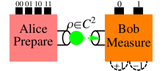
Figure 1: (Color online) The sketch of $2\rightarrow 1$ quantum random access code. Alice encodes her randomly chosen 2 classical bits $a\in\{00,01,10,11\}$ into 1 qubit $\rho_{a}$ and sends it to Bob. To decode the required bit, Bob performs some measurement on the received qubit depending on his input bit $y\in\{0,1\}$ with the measurement results denoted as $b\in\{+1,-1\}$ (which in the computational basis can be represented by $b\in\{0,1\}$).

In this work, we focus on the $2\rightarrow 1$ QRAC, which is sketchily depicted in Figure 1 (a more detailed description will be given in next section). Since there exists no entanglement in this model and no classical counterpart, we exploit quantum discord (and geometric measure of discord) to characterize the nonclassical nature of QRACs. Indeed, our analytical results show that the quantum discord is nonzero, and more fascinatingly, reaches the maximal value for the optimal encoding for $2\rightarrow 1$ QRAC. To go deeper into the state encodings, we also step forward to study the dynamical behavior of quantum discord regarding some possible state variations (rotations, in fact). Except for the above-mentioned intrinsic interest of QRACs, we also try to clarify the relationship between the two-dimensional quantum witness Pawlowski2011 ; Gallego2010 ; Brunner2008 and quantum correlation. By numerical evaluations, it has turned out that these two quantities are monotonically related to each other, which may indicate the randomness associated with the dimension witness may originate from nonclassical correlations.

The outline of this paper is as follows. In Sec. II, we briefly review the notations and definitions used throughout this paper. In Sec. III, we turn to analyze the quantum correlations in $2\rightarrow 1$ QRAC, including the original quantum discord and the geometric version. In Sec. IV, we go further to investigate the dynamical behavior of quantum discord with respect to state rotations. Sec. V is devoted to the discussion and conclusion.

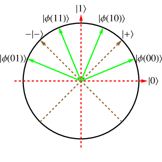
Figure 2: (Color online) Optimal $2\rightarrow 1$ quantum random access coding in $|0\rangle-|1\rangle$ plane representation Hayashi2006 .

II NOTATIONS AND DEFINITIONS

Quantum random access codes. The idea behind QRACs was first raised by Stephen Wiesner Wiesner1983 in 1983 and was labeled as conjugate coding at that time. More than a decade later, these codes were re-discovered by Ambainis et al. in Ref Ambainis1999 ; Ambainis2002 and represented in the standard form: $(n,m,p)$-QRA codings. Here, the notion of $(n,m,p)$-QRACs is adopted to denote the task in which the sender (Alice) encodes $n$ classical bits into $m$-qubit states in order that the receiver (Bob) can recover any one bit of the initial n bits with probability at least $p$. To exhibit the advantage of quantum codings over classical encodings, Ambainis et al. presented an exact example for $\big{(}2,1,\frac{1}{2}(1+\frac{1}{\sqrt{2}})\big{)}$-QRAC and referred to its straightforward generalization to $\big{(}3,1,\frac{1}{2}(1+\frac{1}{\sqrt{3}})\big{)}$-QRAC by Chuang Ambainis1999 , which are just the optimal codings for cases $n=2$ and 3. However, Hayashi et al. proved there is no $(4,1,p)$-QRAC such that $p$ is strictly greater than 1/2 Hayashi2006 (For history and applications about QRACs, we refer the readers to an extended work Ambainis2008 ).

From now on, we concentrate on $2\rightarrow 1$ QRAC. To begin with, let us introduce the $\big{(}2,1,\frac{1}{2}(1+\frac{1}{\sqrt{2}})\big{)}$-QRA coding strategy. Alice encodes her two random bits $a_{1}a_{2}\in\{0,1\}^{2}$ into one qubit $\rho_{a_{1}a_{2}}=|\phi(a_{1}a_{2})\rangle\langle\phi(a_{1}a_{2})|$ where

$$|\phi(00)\rangle =\cos(\frac{\pi}{8})|0\rangle+\sin(\frac{\pi}{8})|1\rangle,$$

$$|\phi(01)\rangle =\cos(\frac{7\pi}{8})|0\rangle+\sin(\frac{7\pi}{8})|1\rangle,$$

$$|\phi(10)\rangle =\cos(\frac{3\pi}{8})|0\rangle+\sin(\frac{3\pi}{8})|1\rangle,$$

$$|\phi(11)\rangle =\cos(\frac{5\pi}{8})|0\rangle+\sin(\frac{5\pi}{8})|1\rangle,$$ (1)

To extract the required bit, Bob performs the two projective measurements as follows

$$M_{1} =\{M_{0}^{0}=|0\rangle\langle 0|,\,M_{0}^{1}=|1\rangle\langle 1|\},$$

$$M_{2} =\{M_{1}^{0}=|+\rangle\langle+|,\,M_{1}^{1}=|-\rangle\langle-|\},$$ (2)

with $|\pm\rangle=\frac{1}{\sqrt{2}}(|0\rangle\pm|1\rangle)$. In Figure 2, we explicitly illustrate the optimal state encodings and decodings in $|0\rangle-|1\rangle$ plane representation. It is easy to see that the probability that Bob successfully recovers any of Alice’s two bits is $\cos(\frac{\pi}{8})^{2}=\frac{1}{2}(1+\frac{1}{\sqrt{2}})\approx 0.85$. On the contrary, there exists no $2\rightarrow 1$ classical encoding for any $p>\frac{1}{2}$ Ambainis1999 . The gap between quantum and classical encodings motivates us to investigate the quantum correlations in quantum encodings, which is very likely responsible for the advantage over classical encodings. In fact, Alice’s coding strategy can be written as a mixture of four product states

$$\rho_{AB}= \frac{1}{4}(|00\rangle\langle 00|\otimes\rho_{00}+|01\rangle\langle 01|\otimes\rho_{01}$$

$$+|10\rangle\langle 10|\otimes\rho_{10}+|11\rangle\langle 11|\otimes\rho_{11}).$$ (3)

Obviously, there exists no entanglement between the natural bipartite split, and this $4\otimes 2$ classical-quantum state is just our starting point for the later analysis.

Quantum discord. The quantum discord is proposed by Ollivier and Zurek as an informational-theoretical measure of the quantumness of correlations, which originates from the inequivalence of two classically identical expressions of the mutual information in the quantum realm Ollivier2001 . For a given composite system $\rho_{AB}$

$$\mathcal{D}_{A}(\rho):=\mathcal{I}(\rho)-\mathcal{J}(\rho|\{\Pi_{A}^{k}\}),$$ (4)

where $\mathcal{I}(\rho)=S(\rho_{A})+S(\rho_{B})-S(\rho)$ denotes the quantum mutual information, $S(\rho)=-Tr(\rho\log_{2}\rho)$ is the von Neumann entropy, $\rho_{A(B)}=Tr_{B(A)}(\rho)$ represent the reduced states for subsystem A(B) and $\mathcal{J}(\rho|\{\Pi_{A}^{k}\})$ is suggested by Henderson and Vedral as a measure to quantify the classical correlation Henderson2001

$$\mathcal{J}(\rho|\{\Pi_{A}^{k}\}): =S(\rho_{B})-\min_{\{\Pi_{A}^{k}\}}S(\rho|\{\Pi_{A}^{k}\}),$$

$$=S(\rho_{B})-\min_{\{\Pi_{A}^{k}\}}p_{k}S(\rho_{B}^{k}),$$ (5)

where $p_{k}=Tr(\Pi_{A}^{k}\rho)$ and $\rho_{B}^{k}=Tr_{A}(\Pi_{A}^{k}\rho)/p_{k}$, and the minimum is taken over all von Neumann measurements $\{\Pi_{A}^{k}\}$ to eliminate the dependence on specific measurement. Although much endeavor has been devoted to calculating quantum discord for the two-qubit states Luo2008b ; Ali2010 ; Girolami2011 ; Chen2011 , analytical results for high-dimensional systems are rarely to be found in the literature Datta2008 ; Chitambar2011 . To compute the quantum discord of state (II), we should resort to the original formula of discord defined here.

Geometric discord. Based on the Hilbert-Schmidt norm, Dakić et al. introduced the following geometric measure of quantum discord Dakic2010

$$\mathcal{D}^{G}_{A}(\rho):=\min_{\chi\in\Omega}\|\rho-\chi\|^{2},$$ (6)

where $\Omega$ denotes the set of zero-discord states and $\|\rho-\chi\|^{2}=Tr(\rho-\chi)^{2}$ is the square of Hilbert-Schmidt norm. For the two-qubit case, an analytic form of geometric discord can be obtained

$$\mathcal{D}^{G}_{A}(\rho)=\frac{1}{4}(\|\vec{x}\|^{2}+\|T\|^{2}-\lambda_{max}),$$ (7)

where $x_{i}=Tr(\sigma^{A}_{i}\rho)$ are components of the local Bloch vector for subsystem A, $T_{ij}=Tr(\sigma^{A}_{i}\sigma^{B}_{j}\rho)$ are components of the correlation matrix, and $\vec{x}:=(x_{1},x_{2},x_{3})^{t}$, $T:=(T_{ij})$, $\lambda_{max}$ is the largest eigenvalue of the matrix $K=\vec{x}\vec{x}^{t}+TT^{t}$ (here the superscript t denotes transpose).

It is worth mentioning that, Luo and Fu presented a simplified version of the geometric discord Luo2010a

$$\mathcal{D}^{G}_{A}(\rho)=\min_{\Pi_{A}}||\rho-\Pi_{A}(\rho)||^{2},$$ (8)

where the minimum is over all von Neumann measurements $\Pi_{A}=\{\Pi_{A}^{k}\}$ on subsystem A. Following the treatment method in Luo2010a , the authors of Ref. Rana2012 and Hassan2012 derived a tight lower bound to the geometric discord of arbitrary $m\otimes n$ states

$$\mathcal{D}^{G}_{A}(\rho)\geq\frac{2}{m^{2}n}(\|\vec{x}\|^{2}+\frac{2}{n}\|T\|^{2}-\sum_{i=1}^{m-1}\lambda_{i}^{\downarrow}),$$ (9)

where $\lambda_{i}^{\downarrow}$ are the eigenvalues of $G=\vec{x}\vec{x}^{t}+\frac{2TT^{t}}{n}$ listed in decreasing order (counting multiplicity) and here $\vec{x}=(x_{1},x_{2},...,x_{m})^{t}$, $T=(T_{ij})$ are given by

$$x_{i} =\frac{m}{2}Tr(\rho\tilde{\lambda_{i}}\otimes I_{n})=\frac{m}{2}Tr(\rho_{A}\tilde{\lambda_{i}}),$$

$$T_{ij} =\frac{mn}{4}Tr(\rho\tilde{\lambda_{i}}\otimes\tilde{\lambda_{j}}).$$ (10)

with $\tilde{\lambda_{i}},\tilde{\lambda_{j}}$ being the generators of $SU(d)$ for corresponding dimension $d=m,n$ generator1 . It is remarkable that the lower bound in Eq. (9) is saturated by all $2\otimes n$ states (with the measurement on the qubit) Rana2012 ; Hassan2012 (the same result was also obtained in Ref. Vinjanampathy2012 ). This analytical formula can be directly applied to our case.

III CORRELATION ANALYSIS IN QRAC

Equipped with these concepts and formulas, we are now in the position to analyze the quantum correlation in $2\rightarrow 1$ QRAC, measured by quantum discord (QD) and geometric measure of discord (GD) respectively.

III.1 Quantum discord

First, we notice that state (II) (an $8\times 8$ matrix in fact) can be cast into a block diagonal matrix

$$\rho_{AB}=\left(\begin{array}[]{cccc}\rho_{00}&0&0&0\\ 0&\rho_{01}&0&0\\ 0&0&\rho_{10}&0\\ 0&0&0&\rho_{11}\end{array}\right),$$ (11)

where

$$\rho_{00} =\frac{1}{2}\left(\begin{array}[]{cc}1+\cos\frac{\pi}{4}&\sin\frac{\pi}{4}\\ \sin\frac{\pi}{4}&1-\cos\frac{\pi}{4}\end{array}\right),$$ (14)

$$\rho_{01} =\frac{1}{2}\left(\begin{array}[]{cc}1+\cos\frac{7\pi}{4}&\sin\frac{7\pi}{4}\\ \sin\frac{7\pi}{4}&1-\cos\frac{7\pi}{4}\end{array}\right),$$ (17)

$$\rho_{10} =\frac{1}{2}\left(\begin{array}[]{cc}1+\cos\frac{3\pi}{4}&\sin\frac{3\pi}{4}\\ \sin\frac{3\pi}{4}&1-\cos\frac{3\pi}{4}\end{array}\right),$$ (20)

$$\rho_{11} =\frac{1}{2}\left(\begin{array}[]{cc}1+\cos\frac{5\pi}{4}&\sin\frac{5\pi}{4}\\ \sin\frac{5\pi}{4}&1-\cos\frac{5\pi}{4}\end{array}\right),$$ (23)

The spectrum of $\rho_{AB}$ is $\{1/4,1/4,1/4,1/4,0,0,0,0\}$ (later we will see this spectrum remains invariant under arbitrary state rotations). Moreover, note that the following relations hold

$$\sin(\frac{\pi}{4})+\sin(\frac{3\pi}{4})+\sin(\frac{5\pi}{4})+\sin(\frac{7\pi}{4})=0,$$

$$\cos(\frac{\pi}{4})+\cos(\frac{3\pi}{4})+\cos(\frac{5\pi}{4})+\cos(\frac{7\pi}{4})=0,$$ (24)

Thus the reduced state $\rho_{B}=\frac{1}{4}(\rho_{00}+\rho_{01}+\rho_{10}+\rho_{11})=\frac{1}{2}I$. Since the measurement is performed on the qubit (subsystem B), we need to evaluate the reduced states of subsystem A conditioned on the measurements.

To go through all possible one-qubit projective measurements, we adopt the projectors $\Pi_{\pm}=\frac{1}{2}(I\pm\vec{a}\cdot\vec{\sigma})$ with $|\vec{a}|^{2}=a_{1}^{2}+a_{2}^{2}+a_{3}^{2}=1$ and $\vec{\sigma}=(\sigma_{1},\sigma_{2},\sigma_{3})$ the standard Pauli matrices. Accordingly, the post-measurement states are (in terms of the computational basis $\{|00\rangle,|01\rangle,|10\rangle,|11\rangle\}$)

$$\rho_{A}^{+} =\frac{1}{2}\mathbf{diag}\{P_{00}^{+},P_{01}^{+},P_{10}^{+},P_{11}^{+}\},$$

$$\rho_{A}^{-} =\frac{1}{2}\mathbf{diag}\{P_{00}^{-},P_{01}^{-},P_{10}^{-},P_{11}^{-}\},$$ (25)

where

$$P_{00}^{\pm} =\frac{1}{4}\left[2\pm 2\big{(}a_{1}\sin\frac{\pi}{4}+a_{3}\cos\frac{\pi}{4}\big{)}\right],$$

$$P_{01}^{\pm} =\frac{1}{4}\left[2\pm 2\big{(}a_{1}\sin\frac{7\pi}{4}+a_{3}\cos\frac{7\pi}{4}\big{)}\right],$$

$$P_{10}^{\pm} =\frac{1}{4}\left[2\pm 2\big{(}a_{1}\sin\frac{3\pi}{4}+a_{3}\cos\frac{3\pi}{4}\big{)}\right],$$

$$P_{11}^{\pm} =\frac{1}{4}\left[2\pm 2\big{(}a_{1}\sin\frac{5\pi}{4}+a_{3}\cos\frac{5\pi}{4}\big{)}\right],$$ (26)

Recalling the Eqs. (III.1), the corresponding probabilities are given as

$$p_{+} =\frac{1}{4}(P_{00}^{+}+P_{01}^{+}+P_{10}^{+}+P_{11}^{+})=\frac{1}{2},$$

$$p_{-} =\frac{1}{4}(P_{00}^{-}+P_{01}^{-}+P_{10}^{-}+P_{11}^{-})=\frac{1}{2},$$ (27)

In addition, for this static case, we observe that $P_{00}^{-}=P_{11}^{+}$, $P_{01}^{-}=P_{10}^{+}$, $P_{10}^{-}=P_{01}^{+}$, and $P_{11}^{-}=P_{00}^{+}$. Therefore, the quantum conditional entropy $S(\rho|\{\Pi_{B}^{k}\})=\sum_{k}p_{k}S(\rho_{A}^{k})=S(\rho_{A}^{+})=S(\rho_{A}^{-})$. Then the quantum discord (before optimization) can be obtained

$$\widetilde{\mathcal{D}}_{B}(\rho) =S(\rho_{B})-S(\rho)+\sum_{k}p_{k}S(\rho_{A}^{k})$$

$$=S(\rho_{A}^{+})-1=-\sum_{i}\frac{1}{2}P_{i}^{+}\log_{2}(\frac{1}{2}P_{i}^{+})-1$$

$$=-\frac{1}{2}\sum_{i}P_{i}^{+}\log_{2}(P_{i}^{+}),$$ (28)

where the sum is over $i=00,01,10,11$.

So far, we arrive at the analytical expression of quantum discord without optimization, and next step is to search through all the parameters involved to find out the minimum value. Note that the spectrums of post-measurement states $\rho_{A}^{\pm}$ are independent of $a_{2}$. Intuitively, it would be a good choice if we let $a_{2}=0$ Datta . Actually, our intuition is correct and the reason for this is as follows. We can define the set of parameters

$$\left\{\begin{array}[]{ccc}a_{1}=\eta\cos\theta,\\ a_{2}=\pm\sqrt{1-\eta^{2}},\\ a_{3}=\eta\sin\theta,\end{array}\right.$$ (32)

with two variables $0\leq\eta\leq 1$ and $\theta\in[0,\pi)$. It is easy to see that $\eta$ turns into a global coefficient before the parentheses in Eqs. (III.1) and the smaller the value of $\eta$, the closer the spectrum of $\rho_{A}^{\pm}$ gets to $\{1/4,1/4,1/4,1/4\}$, which implies $S(\rho_{A}^{\pm})$ will gradually increase. Therefore, it is essential to set $\eta=1$ and then we only need to perform the optimization over one variable $\theta$.

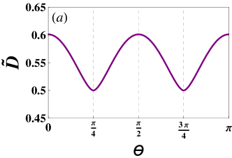
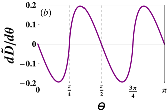
Figure 3: (Color online) The $\widetilde{\mathcal{D}}_{B}(\rho)$ in Eq. (III.1) (a) and the first derivative of $\widetilde{\mathcal{D}}_{B}(\rho)$ (b) as a function of the optimization parameter $\theta$.

Attempting to find the minimum value, we analyze the first derivative of $\widetilde{\mathcal{D}}_{B}(\rho)$, which shows a periodic behavior, as plotted in Figure 3. The data clearly shows that for $\theta=\frac{\pi}{4}$ or $\frac{3\pi}{4}$, $\widetilde{\mathcal{D}}_{B}(\rho)$ reaches the minimum value $\frac{1}{2}$, which corresponds to the spectrum $\lambda(\rho_{A}^{\pm})=\{1/2,1/4,1/4,0\}$. Now we know that the exact value of quantum discord of the optimal $2\rightarrow 1$ QRAC is $\mathcal{D}_{B}(\rho)=\min_{\theta}\widetilde{\mathcal{D}}_{B}(\rho)=\frac{1}{2}$.

III.2 Geometric discord

In this subsection we try to assess the geometric discord. The key point is to represent state (II) in Bloch form, as done in Ref. Rana2012 ; Hassan2012 . First, let us briefly review the $SU(d)$ description of $d$-dimensional density operator. The standard $SU(d)$ generators are natural extensions of the Pauli matrices (for qubits), which are also known as the generalized Gell-Mann matrices (GGM) in higher-dimensional systems generator2 . They are defined as three different types of matrices and for brevity we list these operators in the standard basis here

$$\mathcal{U}_{jk}=|j\rangle\langle k|+|k\rangle\langle j|,$$

$$\mathcal{V}_{jk}=-i(|j\rangle\langle k|-|k\rangle\langle j|),$$

$$\mathcal{W}_{l}=\sqrt{\frac{2}{l(l+1)}}\left(\sum_{j=1}^{l}|j\rangle\langle j|-l|l+1\rangle\langle l+1|\right),$$ (33)

where $1\leq j<k\leq d$ and $1\leq l\leq d-1$.

To be consistent with the notations defined in Section II and also for the sake of simplicity, we swap the subsystems A and B in Eq. (II) and rephrase it as

$$\varrho_{AB}= \frac{1}{4}(\rho_{00}\otimes|00\rangle\langle 00|+\rho_{01}\otimes|01\rangle\langle 01|$$

$$+\rho_{10}\otimes|10\rangle\langle 10|+\rho_{11}\otimes|11\rangle\langle 11|).$$ (34)

Note that the measurements are still performed on the qubit system (here means subsystem A) and this swap procedure has no impact on the final results.

For subsystem A ($d=2$) the $SU(2)$ generators are the standard Pauli matrices, while for subsystem B ($d=4$) the $SU(4)$ generators are a series of $4^{2}-1=15$ matrices generator2 . However, combining the Eqs. (II) (trace operator is involved) with the form of state (III.2), we immediately find that only three diagonal GGM contribute to the calculation. In the standard basis they are given as

$$\mathcal{W}_{1}=\left(\begin{array}[]{cccc}1&0&0&0\\ 0&-1&0&0\\ 0&0&0&0\\ 0&0&0&0\end{array}\right),$$ (39)

$$\mathcal{W}_{2}=\frac{1}{\sqrt{3}}\left(\begin{array}[]{cccc}1&0&0&0\\ 0&1&0&0\\ 0&0&-2&0\\ 0&0&0&0\end{array}\right),$$ (44)

$$\mathcal{W}_{3}=\frac{1}{\sqrt{6}}\left(\begin{array}[]{cccc}1&0&0&0\\ 0&1&0&0\\ 0&0&1&0\\ 0&0&0&-3\end{array}\right),$$ (49)

With these preparations, it is easy to obtain the Bloch vector $\vec{x}$

$$x_{1} =\frac{1}{4}(\sin\frac{\pi}{4}+\sin\frac{3\pi}{4}+\sin\frac{5\pi}{4}+\sin\frac{7\pi}{4})=0,$$

$$x_{2} =0,$$

$$x_{3} =\frac{1}{4}(\cos\frac{\pi}{4}+\cos\frac{3\pi}{4}+\cos\frac{5\pi}{4}+\cos\frac{7\pi}{4})=0,$$ (50)

and the correlation matrix $T$

$$T=\left(\begin{matrix}0&0&\ldots&0&T_{11}&T_{12}&T_{13}\\ 0&0&\ldots&0&T_{21}&T_{22}&T_{23}\\ 0&0&\ldots&0&T_{31}&T_{32}&T_{33}\\ \end{matrix}\right),$$ (51)

where $T$ is a $3\times 15$ matrix and later we will see that actually only 6 entries of $T_{ij}=\frac{2\times 4}{4}Tr(\varrho\sigma_{i}\otimes\mathcal{W}_{j})$ can be nonzero (in this static case there are five)

$$T_{11} =\frac{1}{2}(\sin\frac{\pi}{4}-\sin\frac{7\pi}{4}),$$

$$T_{12} =\frac{1}{2\sqrt{3}}(\sin\frac{\pi}{4}+\sin\frac{7\pi}{4}-2\sin\frac{3\pi}{4}),$$

$$T_{13} =\frac{1}{2\sqrt{6}}(\sin\frac{\pi}{4}+\sin\frac{7\pi}{4}+\sin\frac{3\pi}{4}-3\sin\frac{5\pi}{4}),$$

$$T_{21} =T_{22}=T_{23}=0,$$ (52)

$$T_{31} =\frac{1}{2}(\cos\frac{\pi}{4}-\cos\frac{7\pi}{4})=0,$$

$$T_{32} =\frac{1}{2\sqrt{3}}(\cos\frac{\pi}{4}+\cos\frac{7\pi}{4}-2\cos\frac{3\pi}{4}),$$

$$T_{33} =\frac{1}{2\sqrt{6}}(\cos\frac{\pi}{4}+\cos\frac{7\pi}{4}+\cos\frac{3\pi}{4}-3\cos\frac{5\pi}{4}),$$

Furthermore, we have

$$G=\vec{x}\vec{x}^{t}+\frac{2TT^{t}}{n}=\frac{1}{2}\left(\begin{array}[]{ccc}1&0&0\\ 0&0&0\\ 0&0&1\end{array}\right).$$ (56)

Thus the geometric discord of the optimal $2\rightarrow 1$ QRAC is $\mathcal{D}_{G}=\frac{1}{16}$.

IV DYNAMICAL BEHAVIOR OF QUANTUM DISCORD AND ITS CONNECTION WITH DIMENSION WITNESS

In this section, we go a step further by demonstrating the dynamical behavior of quantum discord (and geometric discord) concerning some possible state rotations. And more importantly, we illustrate the monotonic relationship between the quantum discord and two-dimensional quantum witness Pawlowski2011 ; Li2011 ; Li2012 .

IV.1 Two-state case

To begin with, we first concentrate on the two-state case (see Figure 4). The state rotations can be expressed as

$$\frac{\pi}{8}\rightarrow\frac{\pi}{8}+\delta,\quad\frac{7\pi}{8}\rightarrow\frac{7\pi}{8}-\delta,$$

$$\frac{3\pi}{8}\rightarrow\frac{3\pi}{8}-\delta,\quad\frac{5\pi}{8}\rightarrow\frac{5\pi}{8}+\delta,$$ (57)

It is worth pointing out that since the double angle formula is applied in the above derivation of Eqs. (14), in fact the transformation can be viewed as $\frac{\pi}{4}\rightarrow\frac{\pi}{4}+2\delta,\frac{7\pi}{4}\rightarrow\frac{7\pi}{4}-2\delta,\frac{3\pi}{4}\rightarrow\frac{3\pi}{4}-2\delta,\frac{5\pi}{4}\rightarrow\frac{5\pi}{4}+2\delta$.

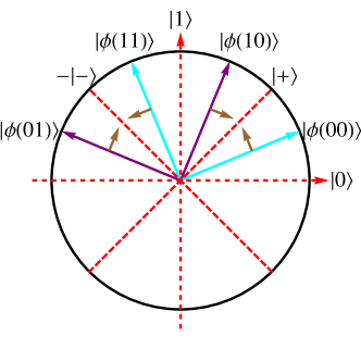
Figure 4: (Color online) State rotations correspond to the two-state case: the orthogonal basis $\{|\phi(00)\rangle,|\phi(11)\rangle\}$ rotates as a unit counterclockwise with the angle $\delta$, while in contrast, another basis $\{|\phi(01)\rangle,|\phi(10)\rangle\}$ rotates as a unit clockwise with the same angle.

Following the original definition of quantum discord, all we need is to evaluate the three terms $S(\rho_{AB})$, $S(\rho_{B})$ and $\sum_{k}p_{k}S(\rho_{A}^{k})$ under this transformation. One can easily check that the spectrum of $\rho_{AB}$ remains unchanged and in fact $\rho_{B}$ also keeps invariant because the following relations still hold

$$\sum_{i=1}^{4}\sin(\phi_{i})=\sum_{i=1}^{4}\cos(\phi_{i})=0,$$ (58)

with $\phi_{0}=\frac{\pi}{4}+2\delta$, $\phi_{1}=\frac{7\pi}{4}-2\delta$, $\phi_{2}=\frac{3\pi}{4}-2\delta$, $\phi_{3}=\frac{5\pi}{4}+2\delta$. For the same reason, we have $p_{+}=p_{-}=\frac{1}{2}$ again. Therefore, the formula (III.1) can still be employed in this case, and of course the optimization can be preformed only over $\theta$. As for geometric discord, it turns out that the coefficients in Eq. (III.2) and (A) stay the same and we only need to take the angle transformation into consideration. The geometric discord can be analytically obtained

$$\mathcal{D}_{G} =\frac{1}{8}\left\{1-\max\big{[}\sin^{2}(\frac{\pi}{4}+2\delta),\cos^{2}(\frac{\pi}{4}+2\delta)\big{]}\right\}$$

$$=\frac{1}{16}(1-|\sin 4\delta|).$$ (59)

Obviously, when $\delta=0$, $\mathcal{D}_{G}$ reduces to the static situation.

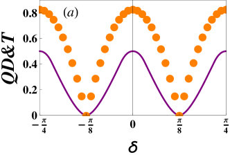
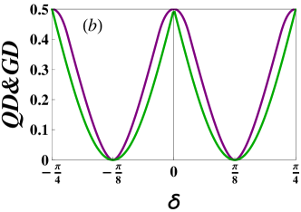
Figure 5: (Color online) (a)The comparison between quantum discord (purple solid line) and two-dimensional quantum witness (orange dotted line); (b)the comparison between quantum discord (purple solid line) and geometric discord (green solid line). Note that here we actually plot $T-2$ T-2 and $8\mathcal{D}_{G}$ for clarity.

In our previous work Li2011 ; Li2012 , Li et al. proposed a semi-device-independent random-number expansion scenario with the help of $2\rightarrow 1$ QRAC protocol, where the genuine randomness is certified by the two-dimensional quantum witness violation $T$, which was first introduced by M. Pawłowski and N. Brunner Pawlowski2011

$$T\equiv +E_{00,0}+E_{00,1}+E_{01,0}-E_{01,1}$$

$$-E_{10,0}+E_{10,1}-E_{11,0}-E_{11,1}\leq 2\sqrt{2},$$ (60)

where $E_{a_{1}a_{2},y}=P(b=0|a_{1}a_{2},y)$ and $P(b|a,y)=Tr(\rho_{a}M_{y}^{b})$ denotes the probability of Bob finding outcome $b$ when he performed measurement $M_{y}$ and Alice prepared $\rho_{a}$. The bound $T\leq 2\sqrt{2}$ corresponds to the maximum violation of 2-dimensional witness in the semi-device-independent black-box scenario, which is somewhat similar to the maximal CHSH-inequality violation ($2\sqrt{2}$) by two-qubit states. Here, “semi-device-independent” indicates only a two-dimensional system will be considered in this protocol and this bound $T\leq 2\sqrt{2}$ was numerically presented in Ref. Li2011 . When $T=2\sqrt{2}$, it implies that Bob’s success probability of guessing any one bit of Alice’s initial 2 bits is

$$P_{B}=\frac{2+\sqrt{2}}{4}\approx 0.85.$$ (61)

which is optimal in $2\rightarrow 1$ QRAC. For more details about dimension witnesses, We would like to draw the reader’s attention to the seminal paper by R. Gallego et al. Gallego2010 . Actually, Eq. (IV.1) is a straightforward extension of the witness $I_{3}$ of Ref. Gallego2010 .

Within the $2\rightarrow 1$ QRAC framework, we make two types of comparisons: (i) between QD and two-dimensional quantum witness violation $(T-2)$ (Figure 5 (a)); (ii) between QD and GD (Figure 5 (b)). From these plots, there are several points worth highlighting: (1) witness $T$ is monotonically related to QD, which implies the randomness guaranteed by $T$ may have some connection with quantum correlations. However, we also notice that only when $T>2.64$ the positive amount of randomness can be achieved Li2011 ; (2) GD behaves highly monotonically with respect to QD as well, and it indicates that in this case GD can also be viewed as a faithful measure of quantum correlation; (3) All the maximum or minimum values of these three quantities occur simultaneously. For instance, when the rotation angle $\delta=\frac{\pi}{8}$, the orthogonal basis $\{|\phi(00)\rangle,|\phi(11)\rangle\}$ and $\{|\phi(01)\rangle,|\phi(10)\rangle\}$ coincide at $\{|+\rangle,|-\rangle\}$. Accordingly, the initial state $\rho_{AB}$ reduces to a classical-classical state Piani2008 , which contains only classical correlations and no quantum correlations; (4) Finally, we would like to point out that if one of the encoding states crosses the other due to the rotations, the state ordering (encoding) must make corresponding changes. It is crucial for the calculation of $T$.

IV.2 Arbitrary rotations in $|0\rangle-|1\rangle$ plane

In fact, we can numerically obtain dimension witness $T$ and quantum discord once the four rotation angles (corresponding to the four encoding states) are specific, applying the above algorithms raised in this paper. Analytical relationship can hardly be achieved and this dilemma is mainly due to the definition and mathematical treatment of dimension witness $T$, since too many variables are involved in the optimization process. Actually, in some earlier papers Gallego2010 ; Brunner2008 , this difficulty has already been pointed out and they numerically derived upper-bounds of dimension witnesses, using semi-definite programming (SDP) to solve the optimization problem.

We also note that one can obtain an analytic expression of geometric discord for the specific rotation discussed in subsection A. Meanwhile, we realize that geometric discord may be more appropriate for characterizing quantum correlations with respect to our topic, not only because of its mathematical simplicity but also due to its definition: geometric discord is defined from the geometric point of view. Therefore, we attempt to give the analytic formulation of geometric discord for arbitrary rotations in real $|0\rangle-|1\rangle$ plane. The arbitrary rotation can be represented as

$$\frac{\pi}{8}\rightarrow\frac{\pi}{8}+\delta_{1},\quad\frac{7\pi}{8}\rightarrow\frac{7\pi}{8}+\delta_{2},$$

$$\frac{3\pi}{8}\rightarrow\frac{3\pi}{8}+\delta_{3},\quad\frac{5\pi}{8}\rightarrow\frac{5\pi}{8}+\delta_{4},$$ (62)

This calculation is tedious and lengthy, but with the help of mathematical softwares, we found that some terms can be eliminated and some terms can be collected. Finally we arrive at the following three eigenvalues of $G=\vec{x}\vec{x}^{t}+\frac{2TT^{t}}{n}$

$$\lambda_{1}= \frac{4-\sqrt{2\Delta}}{8},$$

$$\lambda_{2}= 0,$$

$$\lambda_{3}= \frac{4+\sqrt{2\Delta}}{8},$$ (63)

where $\Delta=2+\cos 4(\delta_{1}-\delta_{4})+\cos 4(\delta_{2}-\delta_{3})-\cos 4(\delta_{1}-\delta_{2})-\cos 4(\delta_{1}-\delta_{3})-\cos 4(\delta_{2}-\delta_{4})-\cos 4(\delta_{3}-\delta_{4})$. It is easy to see that the example in subsection A can be rephrased as $\delta_{1}=\delta,\delta_{2}=-\delta,\delta_{3}=-\delta,\delta_{4}=\delta$. Inserting these equations into the general formula, we can get

$$\lambda^{\prime}_{1}= \frac{1-|\sin 4\delta|}{2},$$

$$\lambda^{\prime}_{2}= 0,$$

$$\lambda^{\prime}_{3}= \frac{1+|\sin 4\delta|}{2},$$ (64)

which exactly coincides with Eq. (IV.1). Hence, the geometric discord for arbitrary rotations can be obtained

$$\mathcal{D}_{G}=\frac{1}{8}(1-\lambda_{3})=\frac{1}{8}\lambda_{1}=\frac{4-\sqrt{2\Delta}}{64}.$$ (65)

It is remarkable that geometric discord reaches $\frac{1}{16}$ when $\delta_{1}=\delta_{2}=\delta_{3}=\delta_{4}=0$, which is compatible with the optimal encoding strategy. However, for arbitrary state encodings in Bloch sphere, we have performed numerical simulations in a more general situation of the model and our results indicate that maximal geometric discord can not coincide with optimal $2\rightarrow 1$ QRAC. More details about numerical simulations are available in the Appendix.

V DISCUSSION AND CONCLUSION

In this paper we have investigated quantum discord (and geometric discord) in quantum random access codes, which have proved to be a valuable tool for a variety of applications in quantum information theory. We notice that this model involves no entanglement at all and thus the usefulness of this protocol can not be attributed to entanglement. However, our analysis highlights the presence of quantum discord in this protocol and it indicates that quantum discord would be thought of as figure of merit for characterizing quantum nature in this communication model since this model has no classical counterparts.

In two-state case, we explicitly elaborate the relations between quantum discord and two-dimensional quantum witness following the method in Pawlowski2011 ; Li2011 ; Li2012 . Our results show that the two quantities are monotonically related to each other and achieve the maximum or minimum values under the same conditions. In addition, we also find that the geometric discord behaves highly monotonically with respect to quantum discord in this case.

Furthermore, we derive an explicit analytical expression of the geometric discord if we restrict to state encodings in real $|0\rangle-|1\rangle$ plane and it turns out that geometric discord reaches the maximal value for the optimal encoding strategy. However, our numerical simulations reveal that for arbitrary state encodings in Bloch sphere, maximal geometric discord could not coincide with optimal $2\rightarrow 1$ QRAC, which is in sharp contrast to the situation we encounter in $|0\rangle-|1\rangle$ plane. A clearer picture between quantum discord and dimension witnesses remains an open question and deserves more investigation.

In view of these findings, we should note that there are many other interesting issues that remain to be addressed: (i) it would be worthy of investigation in $3\rightarrow 1$ QRAC, since Li et al. pointed out that the $3\rightarrow 1$ QRAC is the most efficient semi-device-independent randomness-generation protocol known Li2012 . (ii) although in two-state case witness $T$ is monotonically related to quantum discord, we notice that only when $T>2.64$ the positive amount of randomness can be achieved Li2011 . Recently, experimental device-independent tests of classical and quantum dimensions have been put forward Ahrens2012 ; Hendrych2012 . It is desirable to clarity the intrinsic connection between dimension witnesses and quantum correlations. (iii) the relationship between quantum discord and geometric discord may need further investigation, especially in high-dimensional systems. Since the validity of geometric discord as a good measure for the quantumness of correlations has been questioned Piani2012 , its operational meaning urgently need to be uncovered (a recent example has been reported by Streltsov et al. Streltsov2012b ).

Appendix A Numerical simulations in Bloch sphere

Here we consider the geometric discord as a figure of merit. The key point to evaluate geometric discord is to find the three eigenvalues $\lambda_{1},\lambda_{2},\lambda_{3}$ of the matrix

$$G=\vec{x}\vec{x}^{t}+\frac{2TT^{t}}{n},$$ (66)

with $\lambda_{1},\lambda_{2},\lambda_{3}\in[0,1]$ and $TrG=\lambda_{1}+\lambda_{2}+\lambda_{3}=1$. Indeed, for arbitrary encodings $|0\rangle-|1\rangle$ plane, we have analytically obtained that

$$\lambda_{1}= \frac{4-\sqrt{2\Delta}}{8},$$

$$\lambda_{2}= 0,$$

$$\lambda_{3}= \frac{4+\sqrt{2\Delta}}{8},$$ (67)

where $\Delta=2+\cos 4(\delta_{1}-\delta_{4})+\cos 4(\delta_{2}-\delta_{3})-\cos 4(\delta_{1}-\delta_{2})-\cos 4(\delta_{1}-\delta_{3})-\cos 4(\delta_{2}-\delta_{4})-\cos 4(\delta_{3}-\delta_{4})$. It is worth noting that one of the eigenvalues is zero (which indicates that $\lambda_{1}\leq\frac{1}{2}$ and $\lambda_{3}\geq\frac{1}{2}$) and the geometric discord can be given as

$$\mathcal{D}_{G}=\frac{1}{8}(1-\lambda_{3})=\frac{1}{8}\lambda_{1}=\frac{4-\sqrt{2\Delta}}{64}\leq\frac{1}{16},$$ (68)

where the equality is satisfied if $\delta_{1}=\delta_{2}=\delta_{3}=\delta_{4}=0$, which just corresponds to the optimal encodings. However, if we consider arbitrary encodings in Bloch sphere, the situation becomes technically hard to solve and we can only turn to numerical simulations. Before proceeding, it is intuitive to think that for arbitrary encodings probably the three eigenvalues are all greater than 0 since more variables are involved in this case. If so, we can expect that

$$\mathcal{D}_{G}=\frac{1}{8}\left(1-\max[\lambda_{1},\lambda_{2},\lambda_{3}]\right)\leq\frac{1}{12}.$$ (69)

where the equality is satisfied if $\lambda_{1}=\lambda_{2}=\lambda_{3}=\frac{1}{3}$.

In this situation, the Bloch sphere representation can be employed as a very useful tool to run the simulations. A pure qubit state can be represented as

$$|\psi\rangle=\cos\frac{\theta}{2}|0\rangle+e^{i\varphi}\sin\frac{\theta}{2}|1\rangle,$$ (70)

where $\theta\in[0,\pi]$ and $\varphi\in[0,2\pi]$. The Bloch vector for state (70) is $\vec{r}=(x,y,z)$, where the coordinates are given by

$$\left\{\begin{array}[]{ccc}x=\sin\theta\cos\varphi,\\ y=\sin\theta\sin\varphi,\\ z=\cos\theta,\end{array}\right.$$ (74)

Since the phase factor $\varphi$ is involved in the representation, the four encoding states may not lie in the same plane. However, up to local unitary equivalence, we can assume that two of the states (for example, $\rho_{00}$ and $\rho_{01}$) are in the $|0\rangle-|1\rangle$ plane (or $x-z$ plane) without loss of generality. Therefore, the four encoding states can be written as

$$|\phi(00)\rangle =\cos(\frac{\pi}{8}+\delta_{1})|0\rangle+\sin(\frac{\pi}{8}+\delta_{1})|1\rangle,$$

$$|\phi(01)\rangle =\cos(\frac{7\pi}{8}+\delta_{2})|0\rangle+\sin(\frac{7\pi}{8}+\delta_{2})|1\rangle,$$

$$|\phi(10)\rangle =\cos(\frac{3\pi}{8}+\delta_{3})|0\rangle+e^{i\varphi_{1}}\sin(\frac{3\pi}{8}+\delta_{3})|1\rangle,$$

$$|\phi(11)\rangle =\cos(\frac{5\pi}{8}+\delta_{4})|0\rangle+e^{i\varphi_{2}}\sin(\frac{5\pi}{8}+\delta_{4})|1\rangle,$$ (75)

where the six parameters $\delta_{1},\delta_{2},\delta_{3},\delta_{4}\in[0,2\pi]$ and $\varphi_{1},\varphi_{2}\in[0,2\pi]$ (see Figure 6).

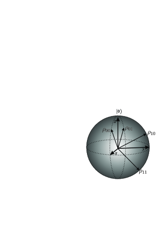
Figure 6: (Color online) The Bloch sphere representation of arbitrary encodings.

After some algebra, we can obtain the Bloch vector $\vec{x}$

$$x_{1}= \frac{1}{4}\bigg{[}\sin(\frac{\pi}{4}+2\delta_{1})+\sin(\frac{7\pi}{4}+2\delta_{2})$$

$$+\sin(\frac{3\pi}{4}+2\delta_{3})\cos\varphi_{1}+\sin(\frac{5\pi}{4}+2\delta_{4})\cos\varphi_{2}\bigg{]},$$

$$x_{2}= \frac{1}{4}\bigg{[}\sin(\frac{3\pi}{4}+2\delta_{3})\sin\varphi_{1}+\sin(\frac{5\pi}{4}+2\delta_{4})\sin\varphi_{2}\bigg{]},$$

$$x_{3}= \frac{1}{4}\bigg{[}\cos(\frac{\pi}{4}+2\delta_{1})+\cos(\frac{7\pi}{4}+2\delta_{2})$$

$$+\cos(\frac{3\pi}{4}+2\delta_{3})+\cos(\frac{5\pi}{4}+2\delta_{4})\bigg{]},$$ (76)

and the correlation matrix $T$

$$T=\frac{1}{2}\left(\begin{matrix}T_{11}&T_{12}&T_{13}\\ T_{21}&T_{22}&T_{23}\\ T_{31}&T_{32}&T_{33}\\ \end{matrix}\right),$$ (77)

where

$$T_{11} =\sin(\frac{\pi}{4}+2\delta_{1})-\sin(\frac{7\pi}{4}+2\delta_{2}),$$

$$T_{12} =\frac{1}{\sqrt{3}}\left[\sin(\frac{\pi}{4}+2\delta_{1})+\sin(\frac{7\pi}{4}+2\delta_{2})-2\sin(\frac{3\pi}{4}+2\delta_{3})\cos\varphi_{1}\right],$$

$$T_{13} =\frac{1}{\sqrt{6}}\left[\sin(\frac{\pi}{4}+2\delta_{1})+\sin(\frac{7\pi}{4}+2\delta_{2})+\sin(\frac{3\pi}{4}+2\delta_{3})\cos\varphi_{1}-3\sin(\frac{5\pi}{4}+2\delta_{4})\cos\varphi_{2}\right],$$

$$T_{21} =0,$$

$$T_{22} =\frac{1}{\sqrt{3}}\left[-2\sin(\frac{3\pi}{4}+2\delta_{3})\sin\varphi_{1}\right],$$ (78)

$$T_{23} =\frac{1}{\sqrt{6}}\left[\sin(\frac{3\pi}{4}+2\delta_{3})\sin\varphi_{1}-3\sin(\frac{5\pi}{4}+2\delta_{4})\sin\varphi_{2}\right],$$

$$T_{31} =\cos(\frac{\pi}{4}+2\delta_{1})-\cos(\frac{7\pi}{4}+2\delta_{2}),$$

$$T_{32} =\frac{1}{\sqrt{3}}\left[\cos(\frac{\pi}{4}+2\delta_{1})+\cos(\frac{7\pi}{4}+2\delta_{2})-2\cos(\frac{3\pi}{4}+2\delta_{3})\right],$$

$$T_{33} =\frac{1}{\sqrt{6}}\left[\cos(\frac{\pi}{4}+2\delta_{1})+\cos(\frac{7\pi}{4}+2\delta_{2})+\cos(\frac{3\pi}{4}+2\delta_{3})-3\cos(\frac{5\pi}{4}+2\delta_{4})\right],$$

First, we resort to mathematical softwares and find that no analytical expressions could be obtained with respect to these six parameters. Then we turn to run simulations by computer programming. Note that we have to go through all the allowed ranges of the six parameters and it is a six-layer loop program, which means that the smaller the step size is, the greater the accuracy obtained but the more time it takes to do the calculations. For example, we first choose the step size as $\frac{\pi}{10}$ and $\frac{\pi}{20}$ (it takes half an hour and about two days respectively to run the simulation). Numerical results (see Table 1) reveal that using smaller step size would cause the geometric discord to get closer and closer to $\frac{2}{3}=0.66\ldots$ (here we consider the normalized geometric discord $8\mathcal{D}_{G}$), as we expected. Note that these values are already larger than $\frac{1}{2}$. Furthermore, we have realized that directly reducing the calculating step size is not a satisfactory strategy since it takes too much time to run the simulation. For instance, if we choose the step size to be $\frac{\pi}{100}$, it will cost us about $\frac{1}{2}\times 10^{6}=5\times 10^{5}$ hours. Therefore, it is more desirable to search around some specific points which have been identified by the simulation, with fine-grained step size (e.g., $\pi\times 10^{-4}$). One set of parameters is listed in Table 1 and the accuracy of the estimate of $\mathcal{D}_{G}$ will gradually increase if we repeat the process for several more iterations (our later runs demonstrated that $8\mathcal{D}_{G}$ indeed approaches $\frac{2}{3}$). As a comparison, we have also obtained the corresponding 2-dimensional quantum witnesses $T$ with with the Levenberg-Marquardt algorithm (see Table 1). From Table 1, we can see that for arbitrary state encodings dimension witness $T$ does not behave monotonically with respect to $\mathcal{D}_{G}$. Besides, if we let $\varphi_{1}=\varphi_{2}=0$ (which means all the four encoding states are in the $|0\rangle-|1\rangle$ plane), simulation results show that $8\mathcal{D}_{G}$ reaches the maximum value $\frac{1}{2}$ when $\delta_{1}=\delta_{2}=\delta_{3}=\delta_{4}=0$, which is compatible with the analytical formula.

Table 1: Numerical results for arbitrary encodings in Bloch sphere.

Step size	$\delta_{1}$	$\delta_{2}$	$\delta_{3}$	$\delta_{4}$	$\varphi_{1}$	$\varphi_{2}$	$8\mathcal{D}_{G}$	$T$
$\frac{\pi}{10}$	$1.40\pi$	$1.90\pi$	$0.30\pi$	$0.70\pi$	$0.60\pi$	$0.40\pi$	0.6090	1.9519
$\frac{\pi}{20}$	$0.35\pi$	$1.90\pi$	$0.45\pi$	$1.55\pi$	$0.60\pi$	$0.35\pi$	0.6431	2.2740
$\pi\times 10^{-4}$	$0.2509\pi$	$0.1980\pi$	$0.3909\pi$	$1.6089\pi$	$0.6928\pi$	$0.3079\pi$	0.6649	1.1658

Finally, we can draw the conclusion that: (i) if we restrict to state encodings in real $|0\rangle-|1\rangle$ plane geometric discord reaches the maximal value ($\frac{1}{16}$) for the optimal encoding strategy; (ii) however, for arbitrary state encodings in Bloch sphere, maximal geometric discord (approaching $\frac{1}{12}$) could not coincide with optimal $2\rightarrow 1$ QRAC, which is in sharp contrast to the situation we encounter in $|0\rangle-|1\rangle$ plane.

References

- (1) H. Ollivier and W. H. Zurek, Phys. Rev. Lett. 88, 017901 (2001).
- (2) L. Henderson and V. Vedral, J. Phys. A 34, 6899 (2001).
- (3) B. Dakić, V. Vedral, and C̆. Brukner, Phys. Rev. Lett. 105, 190502 (2010).
- (4) S. Luo and S. Fu, Phys. Rev. A 82, 034302 (2010).
- (5) S. Luo, Phys. Rev. A 77, 022301 (2008).
- (6) K. Modi, T. Paterek, W. Son, V. Vedral, and M. Williamson, Phys. Rev. Lett. 104, 080501 (2010).
- (7) J. Oppenheim, M. Horodecki, P. Horodecki, and R. Horodecki, Phys. Rev. Lett. 89, 180402 (2002).
- (8) A. Ferraro, L. Aolita, D. Cavalcanti, F. M. Cucchietti, and A. Acín, Phys. Rev. A 81, 052318 (2010).
- (9) A. Datta, A. Shaji, and C. M. Caves, Phys. Rev. Lett. 100, 050502 (2008).
- (10) B. P. Lanyon, M. Barbieri, M. P. Almeida, and A. G. White, Phys. Rev. Lett. 101, 200501 (2008).
- (11) B. Dakic, Y. O. Lipp, X. Ma, M. Ringbauer, S. Kropatschek, S. Barz, T. Paterek, V. Vedral, A. Zeilinger, C̆. Brukner, and P. Walther, arXiv:1203.1629 (2012).
- (12) T. Tufarelli, D. Girolami, R. Vasile, S. Bose, G. Adesso, arXiv:1205.0251 (2012).
- (13) A. Streltsov, H. Kampermann, and D. Bruß, Phys. Rev. Lett. 108, 250501 (2012).
- (14) T. K. Chuan, J. Maillard, K. Modi, T. Paterek, M. Paternostro, and M. Piani, arXiv:1203.1268 (2012).
- (15) C.H. Bennett and G. Brassard, in Proceedings of IEEE International Conference on Computers, Systems and Signal Processing, Bangalore, India (IEEE, New York, 1984), pp. 175-179.
- (16) S. Wiesner, SIGACT News 15, 78 (1983).
- (17) A. Ambainis, A. Nayak, A. Ta-Shma, U. Vazirani, in Proceedings of the 31st Annual ACM Symposium on Theory of Computing (STOC’99), pp. 376-383, 1999.
- (18) A. Ambainis, A. Nayak, A. Ta-Shma, and U. Vazirani, J. ACM 49, 496 (2002).
- (19) M. Hayashi, K. Iwama, H. Nishimura, R. Raymond, and S. Yamashita, New J. Phys. 8, 129 (2006).
- (20) H. Klauck, in Proceedings of the 42nd IEEE Symposium on Foundations of Computer Science (FOCS’01), pp. 288, 2001.
- (21) M. Hayashi, K. Iwama, H. Nishimura, R. Raymond, S. Yamashita, in Proceedings of the 24th International Symposium on Theoretical Aspects of Computer Science (STACS’07), pp. 610-621, 2007.
- (22) M. Pawłowski, T. Paterek, D. Kaszlikowski, V. Scarani, A. Winter, and M. Zukowski, Nature 461, 1101 (2009).
- (23) M. Pawłowski and N. Brunner, Phys. Rev. A 84, 010302(R) (2011).
- (24) H-W. Li, Z-Q. Yin, Y-C. Wu, X-B. Zou, S. Wang, W. Chen, G-C. Guo, and Z-F. Han, Phys. Rev. A 84, 034301 (2011).
- (25) H-W. Li, M. Pawłowski, Z-Q. Yin, G-C. Guo, and Z-F. Han, Phys. Rev. A 85, 052308 (2012).
- (26) S. Pironio et al., Nature (London) 464, 1021 (2010).
- (27) R. Gallego, N. Brunner, C. Hadley, and A. Acín, Phys. Rev. Lett. 105, 230501 (2010).
- (28) N. Brunner, S. Pironio, A. Acín, N. Gisin, A. A. Méthot, and V. Scarani, Phys. Rev. Lett. 100, 210503 (2008).
- (29) A. Ambainis, D. Leung, L. Mancinska, M. Ozols, arXiv:0810.2937 (2008).
- (30) S. Luo, Phys. Rev. A 77, 042303 (2008).
- (31) M. Ali, A. R. P. Rau, and G. Alber, Phys. Rev. A 81, 042105 (2010).
- (32) D. Girolami and G. Adesso, Phys. Rev. A 83, 052108 (2011).
- (33) Q. Chen, C. Zhang, S. Yu, X. X. Yi, and C. H. Oh, Phys. Rev. A 84, 042313 (2011).
- (34) E. Chitambar, arXiv:1110.3057 (2011).
- (35) S. Rana and P. Parashar, Phys. Rev. A 85, 024102 (2012).
- (36) A. S. M. Hassan, B. Lari and P. S. Joag, Phys. Rev. A 85, 024302 (2012).
- (37) F. T. Hioe and J. H. Eberly, Phys. Rev. Lett. 47, 838 (1981); J. Schlienz and G. Mahler, Phys. Rev. A 52, 4396 (1995);
- (38) S. Vinjanampathy and A. R. P. Rau, J. Phys. A 45, 095303 (2012).
- (39) This is exact the way that the author treated this problem in Ref. Datta2008 , but without explanation.
- (40) R. A. Bertlmann and P. Krammer, J. Phys. A 41, 235303 (2008).
- (41) is the classical and quantum boundary for the 2-dimension witness (see Pawlowski2011 ; Gallego2010 ), which means that when the underlying system can only be a quantum state. Therefore, as we expected, the violation of (mathematically denoted as ) can be viewed as a signature of the existence of quantum correlations. This is a key point in our analysis. From figure 5, it is clear to see that “” keeps monotonic with regard to quantum discord. When , the initial state reduces to a classical-classical state, which contains only classical correlations and no quantum correlations. Notice at this moment that and simultaneously.
- (42) M. Piani, P. Horodecki, and R. Horodecki, Phys. Rev. Lett. 100, 090502 (2008).
- (43) J. Ahrens, P. Badzia̧g, A. Cabello, and M. Bourennane, Nature Physics, 8, 592-595 (2012).
- (44) M. Hendrych, R. Gallego, M. Mičuda, N. Brunner, A. Acín and J. P. Torres, Nature Physics, 8, 588-591 (2012).
- (45) M. Piani, arXiv:1206.0231 (2012).
- (46) A. Streltsov, S. M. Giampaolo, W. Roga, D. Bruß, F. Illuminati, arXiv:1206.4075 (2012).