A perturbative approach to the reconstruction of the eigenvalue spectrum of a normal covariance matrix from a spherically truncated counterpart\\[2.0ex]
Filippo Palombia,b††Corresponding author. e–mail: filippo.palombienea.it and Simona Totia \\[2.0ex] aISTAT – Istituto Nazionale di Statistica\\[0.5ex] Via Cesare Balbo 16, 00184 Rome – Italy\\[2.0ex] bENEA – Italian Agency for New Technologies, Energy\\[0.0ex] and Sustainable Economic Development\\[0.5ex] Via Enrico Fermi 45, 00044 Frascati – Italy\\[1.0ex] \dateApril 2014
Abstract
In this paper we propose a perturbative method for the reconstruction of the covariance matrix of a multinormal distribution, under the assumption that the only available information amounts to the covariance matrix of a spherically truncated counterpart of the same distribution. We expand the relevant equations up to the fourth perturbative order and discuss the analytic properties of the first few perturbative terms. We finally compare the proposed approach with an exact iterative algorithm (discussed in Palombi et al. (2017)) in the hypothesis that the spherically truncated covariance matrix is estimated from samples of various sizes.
1 Introduction
The analysis of the probability content of the multivariate normal distribution in finite (or infinite) regions has become a standard problem in probability and statistics since the original works by Ruben, refs. [2, 3, 4, 5]. Other aspects of the problem have been subsequently considered in refs. [6, 7] and more recently in ref.[8]. In a recent paper [1] we studied how the covariance matrix of a multinormal random vector in dimensions, conditioned to a centered spherical domain , relates to the unconditioned covariance matrix . In the same paper we also described practical situations where this kind of distributional truncation occurs.
Owing to the symmetries of the geometrical set-up, and can be shown to commute, i.e. if we let and denote respectively the eigenvalues of and , then and , with the same diagonalizing matrix. The eigenvalues fulfill the equations
| (1.1) |
with and belonging to the class of Gaussian integrals
| (1.2) |
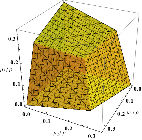
Since and are simultaneously diagonalizable, we can assume and with no loss of generality. We are interested in reconstructing from , namely we aim at solving eqs. (1.1) with respect to under the assumption that and are given (if and are not diagonal and we assume that is known, we can obtain from by diagonalization and use it then for .). As explained in ref. [1], such reconstruction can be of practical importance, for example, in compositional analysis of multivariate log-normal data affected by outlying contaminations. Reconstructing from is equivalent to writing , where is a non-linear operator performing the covariance reconstruction. The existence of follows from the injectivity of . For the sake of completeness, we prove this in App. A. The operator is defined within the convex domain
| (1.3) |
Eq. (1.3) was proposed in ref. [1] as a result of extensive numerical tests. In App. B, we give analytic arguments to support its correctness, although we lack a complete proof. In Fig. 1 (left), we plot for as an illustrative example.
Unfortunately, there exists no general closed-form solution to eqs. (1.1), due to the non-linear character of the problem. For this reason, in ref. [1] we proposed a numerical technique based on a fixed point iteration, whose convergence is ensured by some non-trivial variance and covariance inequalities within [9, 10].
In this paper, we approach eqs. (1.1) from a different standpoint. We move from the observation that a simplified set-up occurs when the eigenvalues are fully degenerate, a case that was first considered by Tallis in ref. [6]. If , by symmetry it follows and the other way round. Eqs. (1.1) reduce in this limit to
| (1.4) |
with denoting the c.d.f. of a -variable with degrees of freedom111With abuse of notation we shall write in place of .. It can be easily checked that is a monotonic increasing function of . In addition, fulfills
| (1.5) |
It follows that eq. (1.4) can be numerically inverted by any root-finding algorithm, provided . We can regard eq. (1.4) as a rough approximation to the original problem. In order to use it when , we must preliminarily define in terms of the components of . One possibility is to average these, i.e. to choose
| (1.6) |
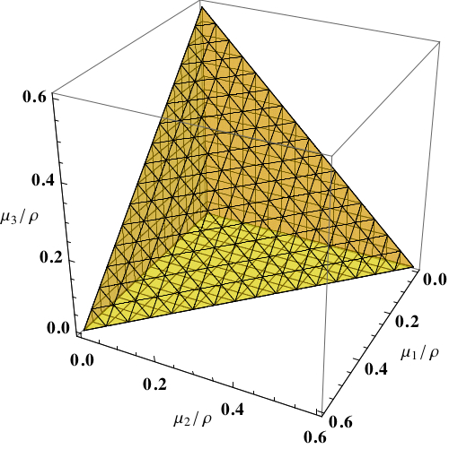
Subject to this choice, we expect to lie somewhere between and . When , eq. (1.4) can be thought of as the lowest order approximation of a perturbative expansion of eqs. (1.1) around the point . If the ratio is not exceedingly large, such expansion is expected to converge quickly. Few perturbative corrections to should be sufficient to guarantee a good level of approximation. In view of eq. (1.6), the inverse operator is defined within the convex domain
| (1.7) |
To allow for a comparison, we also plot for in Fig. 1 (right). Aim of the present paper is to carry out a theoretical study of the perturbative expansion of eqs. (1.1) up to the fourth order and to discuss some analytic aspects of it.
There are several reasons why the suggested perturbative approach can outperform the iterative procedure introduced in ref. [1]. In first place, it can be easily checked that . Accordingly, perturbative approximations to are well defined even when statistical fluctuations in sample space make , provided at least . In this sense, the perturbative approach represents a regularization of the covariance reconstruction problem with respect to the existence of a solution (see sect. 7 of ref. [1] for a detailed discussion of the ill-posedness of the problem).
Secondly, statistical fluctuations of the higher components of are always amplified by eqs. (1.1) as a consequence of the non-linearity and the unboundedness of , sometimes resulting in unacceptably large variances for the higher components of . In the literature of inverse problems, this property is known as the instability of the inverse operator, see for instance ref. [11]. In the framework of perturbation theory, non-linearity arises systematically while increasing the order of the approximation, since each perturbative correction depends non-linearly upon the previous ones. Therefore, by stopping the expansion at different orders we have the possibility to define a class of statistical estimators of , each characterized by its own bias and variance. We find that the variance of the upper (lower) half of the reconstructed eigenvalues increases (decreases) together with the perturbative order, whereas their bias always decreases. In all applications where the upper part of matters, it is therefore possible —at least in principle— to optimize the choice of the perturbative estimator according to one’s specific needs. This provides a regularization of the reconstruction problem with respect to the stability properties of the solution.
Finally, in critical applications requiring reconstructions of the covariance matrix for several values of and/or , it could be important to get fast yet approximate solutions, such as perturbation theory provides, rather than slow yet exact ones. Indeed, the convergence of the fixed point iteration was shown to slow down as or , the rate of the slowing down being polynomial in the former limit and exponential in the latter. Thus, in all situations where or , the use of the fixed point algorithm could be unfavorable.
The plan of the paper is as follows. In sect. 2 we derive some preliminary results concerning the integrals and , which are necessary for a systematic implementation of the perturbative strategy to all orders. In sect. 3 we work out the expansion by means of paper-and-pencil calculations and Maple™ programs (reported in App. C). Sect. 4 is devoted to discussing some analytic properties of the first few perturbative terms, when is chosen as in eq. (1.6). In sect. 5 we simulate the statistical properties of the perturbative estimators of and the iterative one in sample space for a specific choice of the covariance matrix. We finally draw our conclusions in sect. 6.
2 Building blocks in Tallis’ limit
As well known, perturbation theory is an expansion technique around a reference solution, which is assumed to be either calculable or easily computable. Its mathematical structure develops from building blocks which are themselves entirely defined in terms of the reference solution. When it comes to perturbing eqs. (1.1) around , the elementary objects we need to focus on are the Gaussian integrals and their partial derivatives for . In the sequel we refer to this limit as Tallis’ limit.
To begin with, we set-up the notation. Throughout the paper we let denote a set of fully degenerate eigenvalues. Outside Tallis’ limit a convenient axes reshuffling allows us to assume the ordering with no loss of generality (this also follows naturally from assuming , as asserted by Proposition 5 of ref. [1]). We denote a generic Gaussian integral with (not necessarily distinct) indices either by the notation introduced in sect. 1 or by the compact notation , where the generic subscript indicates that the directional index occurs with multiplicity in . Similarly, we denote the order derivative operator with respect to the variances either by the standard symbol or by its compact version . Given , the multiplicity set in unambiguously defined and the other way round. For consistency fulfills the constraint . In case of vanishing multiplicities we omit to write all the corresponding indices. For instance, we write in place of the rather pedantic as well as in place of . Last but not least, we refer the reader to ref. [1] for definitions and properties concerning the truncation operator and its inverse .
Having said that, we start our investigation of Tallis’ limit with a simple proposition, meant to sum up the results of ref. [6]:
Proposition 2.1.
For , …, , we have
| (2.1) |
with
| (2.2) |
Proof.
In order to derive eq. (2.1), we represent in spherical coordinates,
| (2.3) | ||||
Recall that and , with embodying the angular part of the Jacobian of eq. (2.3) and the differentials of the angles , …, . With a bit of algebra we easily arrive at
| (2.4) |
where is just a proportionality factor independent of and . In order to fix , we observe that factorizes into one-dimensional integrals as , corresponding to unconditioned univariate Gaussian moments of orders ,…,, normalized respectively by powers ,…, of the common variance. Hence, we conclude that . ∎
The -c.d.f. is intuitively interpreted as a correction factor incorporating all the effects of integrating Gaussian densities on a finite volume. Obviously, it lessens the value of the integral except for , a limit for which it converges to one.
Whenever Gaussian integrals are expressed in standard notation, eq. (2.1) can be applied only provided the index multiplicities are preliminarily counted. Nevertheless, it is reasonable to expect to be the compact representation of some not yet specified coefficient . By the same argument used above, i.e. by letting , we conclude that the latter is given by
| (2.5) |
Thanks to Isserlis’ Theorem222In mathematical physics the same result is universally known as Wick’s Theorem. [12], can be expressed as a sum of products of Kronecker symbols, namely
| (2.6) |
where the sum includes all distinct ways of partitioning the duplicated set into pairs and the product is over all pairs of a single partition. For later convenience it is worthwhile listing the lowest order coefficients:
| (2.7) | ||||
| (2.8) | ||||
| (2.9) | ||||
Eqs. (2.5)–(2.6) allow us to reformulate Proposition 2.1 as follows:
Corollary 2.1.
Now, in order to take arbitrarily high order derivatives of with respect to the components of , we iterate the basic rule
| (2.11) |
which follows from differentiating under the integral sign. Note that eq. (2.11) is not specifically related to spherical truncations, i.e. it is formally invariant under a reshaping of the truncation surface. It also shows that the differential operator behaves in a simpler manner than when acting on , in that it produces an integer linear combination of Gaussian integrals. For this reason, the recurrence generated by acting on can be derived by first working out the action of the operator on and by then using
| (2.12) |
where the symbols represent unsigned Stirling numbers of the first kind. Eq. (2.12) is a standard result of combinatorial analysis. We refer the reader to exercise 13, chap. 6 of ref. [13] for a proof of it. Iterated applications of the operator generate increasingly involved sums of Gaussian integrals, as asserted by
Proposition 2.2.
For all and , we have
| (2.13) |
with
| (2.14) |
Proof.
The proof is by induction. We first note that and . Hence, for eq. (2.13) agrees with eq. (2.11). Now, suppose that is well represented by eq. (2.13) with as in eq. (2.14). Then,
| (2.15) |
Hence, the proof is complete if we are able to show that fulfills the recurrence
| (2.16) |
To this aim, we first calculate the second term on the r.h.s. as
| (2.17) |
and then we add it to the first one, thus obtaining
| (2.18) |
∎
Nested sums similar to eq. (2.14) are considered for instance in ref. [14], where all cases in study are reduced to closed-form expressions with the help of special numbers, such as binomial coefficients, Stirling numbers, center factorial numbers, etc. Eq. (2.14) looks a bit harder to manage, since the summand is a product of non-homogeneous functions of the sum variables, hence it is not clear whether the nested sums can be ultimately evaluated in closed-form. However, as far as we are concerned, a convenient representation of is provided by
Proposition 2.3.
For all , and , we have
| (2.19) |
with the symbols denoting Stirling numbers of the second kind.
Proof.
We let denote the r.h.s. of eq. (2.19). For , we have and , which equal respectively and . Thus, we just need to prove that fulfills eq. (2.16). To this end, it is sufficient to make use of the basic recursive formulae and . We detail the algebra for the sake of completeness. We start from
| (2.20) |
Then, we add and subtract to the r.h.s. of eq. (2.20). Hence,
| (2.21) |
Since , the second term on the r.h.s. is recognized to be . ∎
In view of ref. [14] it is no surprise that can be represented in terms of Stirling numbers. In addition, the presence of terms such as fits perfectly when combining eq. (2.12) with eq. (2.13). We recall indeed that Stirling numbers of the first and second kind fulfill the identity
| (2.22) |
We have now collected all the ingredients needed to prove the main result of this section, namely
Proposition 2.4.
For , let and denote sets of (not
necessarily distinct) directional indices, i.e. and . We have
(2.23)
In particular, for we have
(2.24)
(2.25)
Proof.
We let and denote the multiplicity sets associated respectively to and , such that , and
| (2.26) |
We recall that and fulfill and for consistency. Using eq. (2.12) times yields
| (2.27) |
Moreover, with the help of eqs. (2.13) and (2.1), eq. (2.27) reduces to
| (2.28) |
As a next step, we evaluate the coefficients , …, in terms of the expressions obtained in Proposition 2.3. Then we make use of eq. (2.22) to make all Stirling numbers disappear. We finally identify and so we arrive at
| (2.29) |
Two additional steps are needed to complete the proof. In first place, we notice that the multiplicity set associated to is . Therefore, by Isserlis’ Theorem we identify . In second place, we observe that ranges from 0 to for , …, . Hence, we recast the r.h.s. of eq. (2.29) to
| (2.30) |
with
| (2.31) |
This multiple sum is easily calculated by iterating the Vandermonde’s convolution . This finally yields . ∎
3 Perturbative expansion
In order to solve eqs. (1.1), perturbation theory prescribes that we interpret and as smooth functions of a parameter , such that and . We must consider as an auxiliary variable, allowing us to pass continuously from Tallis’ limit to the ultimate solution we are seeking. Then, we are requested to expand and in power series of around the point , namely
| (3.1) | ||||||||||
| (3.2) |
For later convenience we let denote the integral ratio . Since depends smoothly upon , it can be analogously expanded in power series of . Thus, eqs. (1.1) read
| (3.3) |
with and for The idea underlying perturbation theory is that we treat separately terms in eq. (3.3) belonging to different perturbative orders, that is to say we equal terms of the same order in on both sides of eq. (3.3) and then we solve one by one the algebraic equations thus obtained. A few caveats must be noticed.
i) Since is an input parameter, we must specify how it enters the Taylor coefficients of the perturbative function . In principle, the assignment can be made in complete freedom. For instance, the choice we adopt in the sequel is to confine to the first-order Taylor coefficient, namely
| (3.4) |
Alternatively, we might spread over all Taylor coefficients of , by letting for instance
| (3.5) |
Both eqs. (3.4) and (3.5) comply with the requirement . It must be noticed, however, that each legitimate splitting of affects differently the convergence properties of the perturbative series of as well as the statistical properties of the truncated series, when is turned into a random variable in sample space. This will be further investigated in sect. 5.
ii) The specific choice of is rather arbitrary: as far as we are concerned with the feasibility of the perturbative expansion, the only requirement to fulfill is that eq. (1.4) be invertible, which is guaranteed provided . We mentioned in sect. 1 that a convenient choice is represented by
| (3.6) |
We shall see shortly what benefits derive from eq. (3.6). Certainly, we have whenever , hence eq. (3.6) is at least a legitimate choice. Indeed, if then from eq. (1.3) it follows that
| (3.7) |
iii) Perturbation theory works only provided the -equations
| (3.8) |
obtained by collecting all the -terms from eq. (3.3), yield an algebraic relation among the Taylor coefficients of which can be solved with respect to . This allows us to represent the latter as a function of the lower order coefficients of together with . If such property is fulfilled, as we argue in a while, then solving eqs. (1.1) perturbatively means solving one after another the systems of equations
| (3.9) |
up to a predefined order . Establishing the level of precision thus achieved is a complicated task, as typical of asymptotic expansions. From a qualitative point of view, the approximation is certainly correct up to -terms. However, that is not a quantitative estimate of the truncation error.
3.1 General structure of the perturbative expansion
Regarding point iii), we notice that the only contributions to depending explicitly upon are and . All other terms are of the form for . These terms depend upon , , …, , but not upon . Indeed, depends upon implicitly via , thus its order derivative with respect to distributes progressively according to the chain rule of differentiation. When evaluating the derivative at , all terms proportional to strictly positive powers of vanish. As a consequence, each surviving term is proportional to a product of Taylor coefficients of , each belonging to . In particular, when an explicit calculation yields
| (3.10) |
To evaluate the first order partial derivatives of , we make use of Propositions 2.1 and 2.4. We have
| (3.11) |
hence eqs. (3.8) reduce to333From now on we omit to write the argument of the -c.d.f. ’s, which is always understood to be .
(3.12)
with
| (3.13) |
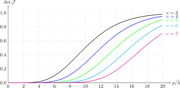
We have obtained a system of linear equations with and representing respectively the unknown vector and the (known) constant. Moreover, the coefficient matrix is the Jacobian of the truncation operator in Tallis’ limit. Its determinant is given by
| (3.14) |
the lower bound in eq. (3.14) following from the inequality , first proved in ref. [15]. We conclude that is non-singular for any finite value of , and therefore eq. (3.12) is unambiguously solved by . Note as well that , hence the invertibility of becomes critical at small values of . By way of example, we show in Fig. 2 a plot of vs. for . Finally, the inverse of can be easily worked out. We have indeed
| (3.15) |
We now discuss the analytic structure of the known term . We have just explained that owing to the chain rule of differentiation, every single contribution to (except for ) includes a partial derivative for some . Expanding this in terms of and yields ratios with numerators made of products of derivatives of and and denominators amounting to some power of . It follows from Propositions 2.1 and 2.4 that can be represented in full generality by
| (3.16) |
with the coefficient having been factored out for later convenience. The subscript prescription has to be understood as a restricting condition on the possible values taken by . For the sake of conciseness, we refer collectively to the ratios as the -ratios and to the coefficients as the -coefs. Evidently the r.h.s. of eq. (3.16) becomes increasingly populated as we increase . The lowest order coefficients are
| (3.17) | ||||
| (3.18) | ||||
Without conditioning the sum to , the number of summands in eq. (3.16) would be (see eq. (1) of ref. [14]). Owing to the restricting condition the actual number of summands is much lower. The intricacy of eq. (3.16) is only apparent: adding separately the indices of all -c.d.f. ’s at numerator and denominator and then subtracting the resulting numbers just yields . Therefore, eq. (3.16) is just a formal way of representing a linear combination of -ratios, where each -c.d.f. has at least degrees of freedom and the overall algebraic sum of degrees of freedom amounts to (with denominators contributing negatively). We remark that this analytic structure is a direct consequence of the chain rule of differentiation together with the results of Propositions 2.1 and 2.4.
Regarding the -coefs, we observe that they do not depend on and can be only determined by explicit calculation. In spite of this, their dependence upon the Taylor coefficients of displays a well defined analytic structure. In order to show this, we rely upon the notions of physical and perturbative dimensions.
i) We assume that has physical dimension of length . To express this we adopt the notation . If we also assume , then it follows . Similarly, we have and . Since , from eq. (3.12) it follows . Hence, eq. (3.16) makes us conclude that
| (3.19) |
As previously explained, the -coefs depend only polynomially upon the Taylor coefficients of . Eq. (3.19) suggests that these polynomials are linear combinations of monomials in and the components of , each monomial having precisely degree .
ii) We define the perturbative dimension of a single monomial as the sum of the perturbative orders of its factors. More precisely, we let , , …, . Thus, for instance, we have . We remark that bears no perturbative dimension, yet it increases the physical dimension of the monomials. Since is the result of the expansion at , it follows that
| (3.20) |
Each monomial contributing to has the same perturbative dimension .
iii) Several monomials contributing to a given -coef have the same perturbative structure and numerical prefactor and differ only by directional indices, e.g. the monomials and . This is a consequence of the index structure of : the products of Kronecker symbols contributing to the r.h.s. of eq. (2.6) contract the indices of the Taylor coefficients of in all possible ways, thus generating an increasing number of new aggregate structures at each order of the expansion. For instance, monomials within the -coefs belonging to the lowest perturbative orders can be grouped according to
| (3.21) | ||||
| (3.22) | ||||
| (3.23) | ||||
In view of the above considerations, we conclude that all -coefs at with can be represented in full generality as linear combinations of all possible products of perturbative structures under the constraints imposed by eqs. (3.19) and (3.20), i.e.
| (3.24) |
with numerical prefactors and perturbative structures fulfilling and . For instance, we have
| (3.25) |
| (3.26) | ||||
Before working out the expansion at a given order, one should list all possible perturbative structures pertaining to that order, such as eqs. (3.25) and (3.1) for respectively. A preliminary identification of all suitable structures is indeed particularly useful in order to identify groups of terms when high order calculations are performed by means of a computer algebra system (CAS), as we shall see in sect. 3.3.
When calculating , many of the coefficients are found to be zero. The non-vanishing ones fulfill the following property:
Proposition 3.1.
For the coefficients fulfill
| (3.27) |
Proof.
We first note that if , then . Therefore, it makes sense to consider eq. (3.12) as with kept fixed. In particular, we have shown previously that . Moreover, as all the -ratios tend to one, thus eq. (3.12) reduces to
| (3.28) |
However, in the same limit , which entails order by order . Hence, we infer that the sum of perturbative structures on the r.h.s. of eq. (3.28) vanishes as . Since in general , we conclude that eq. (3.27) is correct. ∎
The first few orders of the perturbative expansion can be worked out with little algebraic effort. Doing the calculations is useful to familiarize with the general structure discussed so far. The order of the expansion has been discussed in sect. 1. We can focus on the perturbative corrections to it. From now on we assume that has Taylor coefficients given by eq. (3.4).
3.2 Perturbative expansion at
Equations have the explicit form
| (3.29) |
Since , the only term we need to calculate is
| (3.30) |
Actually, we have calculated the first order partial derivatives of in eq. (3.11). Thus, we have
| (3.31) |
whence we infer . Choosing yields an important simplification:
Proposition 3.2.
If , then .
Proof.
It is sufficient to add side by side all eqs. (3.31) for to get
| (3.32) |
Since the quantity in square brackets is strictly positive, we conclude that . ∎
As can be easily understood, having results in a huge simplification of the algebra. Indeed, belongs to many perturbative structures contributing to for . For instance, the set of structures given in eq. (3.25) is reduced to only two elements in place of four when , while the one given in eq. (3.1) is reduced to six elements in place of twelve.
3.3 Perturbative expansion at
The subleading correction is obtained from the equations
| (3.33) |
Most of the contributions to the three terms on the r.h.s. are worked out easily at this point. For instance, we have
| (3.34) |
| (3.35) |
To keep things general, we make no assumptions on here. Accordingly, we retain all -ratios proportional to powers of . The evaluation of the second derivatives requires a few pages of tedious algebraic work, which we cannot detail. The result of the calculations is given by
| (3.36) |
We notice that all four structures listed in eq. (3.25) contribute to the -coefs .
In Table 1 we collect the coefficients . Instead of naming rows and columns respectively according to the values of and the triples , for the sake of readability we identify each table entry by the perturbative-structure and the -ratio it refers to. This way of tabulating coefficients becomes particularly informative at higher orders. We observe that adding the entries of each table row yields zero, in accordance with eq. (3.27).
3.4 Perturbative expansion at higher orders
Paper-and-pencil calculations become prohibitively expensive at higher orders. Fortunately, it is not difficult to work out the algebra with the assistance of a CAS. For the reader’s convenience, in App. C we attach some essential and correctly working Maple™ procedures, which help work out the algebra. The code is split into three blocks, that we shortly review.
The first code block (C.1) contains a procedure Delta(), which computes the coefficient . The procedure argument is assumed to be a list of nonnegint items; alternatively the procedure returns unevaluated. The input list is first sorted in ascending order, then the multiplicity set is identified. The procedure computes the r.h.s. of eq. (2.2) and returns its numerical value.
The second code block (C.2) performs the algebraic work related to the perturbative expansion of eqs. (1.1). Before submitting it to evaluation, the user is assumed to assign a nonnegint variable v representing the number of dimensions, and a nonnegint variable n 4 representing the highest perturbative order processed by the program. The code block starts with a pair of procedures, DerAlpha() and DerAlphak(), which encode respectively eqs. (2.24) and (2.25). Then, it performs a Taylor expansion of the r.h.s. of eqs. (1.1) up to . Taylor coefficients are stored within indexable objects h[j,k], the indices j and k representing respectively the perturbative order and the physical direction. At this stage, h[j,k] includes a sum of potentially many terms. The summands contain derivatives of and , which are purely symbolic objects at this stage. Their evaluation requires sequences of prescriptions, stored within the variables C0A, C0Ak,…, C4A, C4Ak. Algebraic simplifications are performed in the last few lines, where partial results are stored within indexable objects h00,…, h10, so as to allow for an offline analysis of the single steps.
The third code block (C.3) illustrates in a specific case a numerical technique which we have devised for the determination of the coefficients . The code processes the coefficients corresponding to and , i.e. those entering the -coef multiplying the -ratio . It also assumes . As previously discussed, this simplifies the basis of perturbative structures to
| (3.37) |
The algebraic sum pointed to by h10[3,k] at the end of the second code block has no knowledge of these structures. In order to identify them within h10[3,k], we need to group terms properly. Instead of proceeding at an algebraic level, which would be computationally demanding, we adopt a numerical approach, based on the use of eq. (3.24) as a square linear system fulfilled by the coefficients . Having subtracted from h10[3,k] all contributions appearing in eq. (3.10), we extract from it all terms proportional to , whose sum amounts to . Then, for each we assign and random values (chosen so that ), from which we compute , …, and . The random matrix thus obtained is non-singular, hence eq. (3.10) can be solved with respect to . The solution is independent of the random numbers generated. This represents a strong signal that our determination is correct, yet a real check consists of an algebraic comparison between the reconstructed coefficient and the one extracted from h10[3,k]. In Tables 2 and 3 we report the coefficients and under the assumption .
4 Properties of the first few perturbative coefficients
So far we have focused on formal aspects of the perturbative expansion of with the aim of proving its theoretical and computational feasibility. To establish the level of accuracy reached in approximating the reconstruction operator by a handful of perturbative contributions, we need to investigate some analytic properties of the perturbative coefficients of .
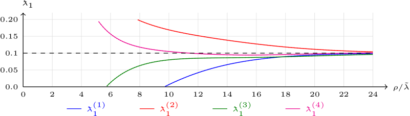
Hereinafter we consider perturbative series truncated at different orders, for which we adopt the notation
| (4.1) |
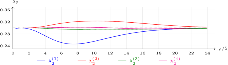
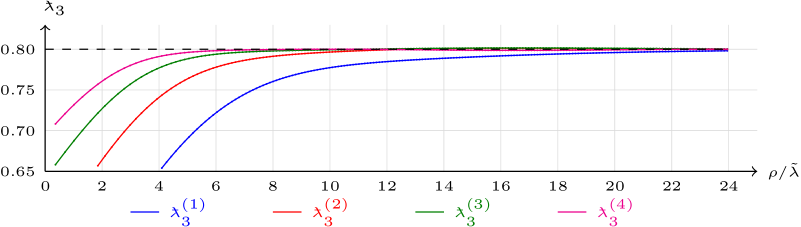
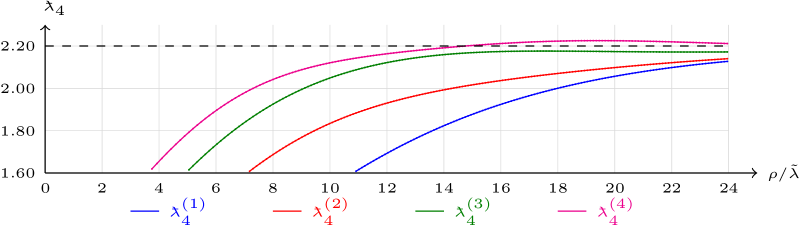
Fig. 3 shows an illustrative example of perturbative reconstructions at . We concentrate on it in the present and next sections. The plots in Fig. 3 have been produced as follows. First of all, in order to test perturbation theory on eigenvalues characterized by a relatively large ratio , we have chosen as the eigenvalue set to reconstruct (accordingly, we have , yielding a highly asymmetric Gaussian ellipsoid). By means of numerical techniques detailed in ref. [1], we have then computed for several values of . In correspondence with each pair we have finally reconstructed up to the fourth perturbative order, having chosen in all cases . We notice from the plots that in most cases the error made by truncating the expansion at a given order increases for lower values of . Moreover, the error is larger for eigenvalues at the extremes of the eigenvalue set and milder in the center of it. We also notice that the convergence pattern for the lower eigenvalues is radically different than for the higher ones. Indeed, the perturbative series of and converges with alternate signs, while the perturbative series of and displays a monotonic character.
In order to explain the observed behavior, we first concentrate on the leading contribution . If fulfills the constraint , a solution to eq. (1.4) exists for all pairs with . We can consider as a function of at fixed . The analytic form of tells us that . Moreover, we know that provided . Since , by continuity we conclude that
| (4.2) |
At sufficiently large the above inequality holds true with and being respectively replaced by and , where is such that .
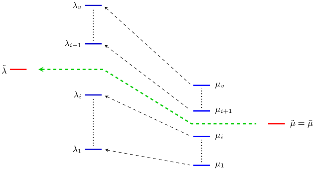
Eq. (4.2) does not tell where is placed in relation to the full eigenvalue spectrum. To find such an estimate, we can resort to eq. (24) of ref. [1]. Based on arguments which are completely analogous to those used therein, we arrive easily at
| (4.3) |
with denoting the Kummer function
| (4.4) |
As a consequence of the asymptotic limit and (see e.g. chap. 13 of ref. [16]), we have
| (4.5) | |||
| (4.6) |
we conclude that if is sufficiently large, then . As intuitively expected, non–linear effects are mitigated in the region of weak truncation. The situation is qualitatively depicted in Fig. 4.
We now consider the first few corrections to . In general, as far as we are concerned with their numerical computation, we can limit ourselves to solve eqs. (3.16) one after another by means of a linear solver. Nevertheless, the matrix structure of is simple. The off–diagonal entries are all the same, independently of the matrix indices. This allows us to invert eqs. (3.16) analytically. When the expression thus obtained has several contributions, we hardly find it better than its numerical computation. Yet, this is not the case with the first few perturbative corrections, of which we want to estimate the range of variation.
Since is either index–free or dependent upon via monomials with , the only algebraic ingredients we need for the analytic inversion of eqs. (3.16) are the sums
| i) | (4.7) | ||||
| ii) | |||||
| (4.8) | |||||
where is defined in analogy with eqs. (3.21)–(3.23). We are now ready to work out the algebra. In first place, a straightforward calculation yields
| (4.9) |
Hence, we infer that
| (4.10) |
We recognize that the first perturbative correction to the leading term is positive for the higher eigenvalues and negative for the lower ones.
The algebraic evaluation of the second perturbative correction to is as easy as the first one, yet estimating its range of variation is somewhat more difficult. In this case we let from the very beginning. Under this assumption, we see that the r.h.s. of eq. (3.36) reduces to a linear combination of four terms, namely
| (4.11) | ||||||
| (4.12) | ||||||
| (4.13) | ||||||
Correspondingly, the solution of eq. (3.36) is the sum of four contributions:
| (4.14) | ||||
| (4.15) |
| (4.16) | ||||
| (4.17) | ||||
| (4.18) |
Hence, we have
| (4.19) |
Since , the first contribution to the r.h.s. is certainly positive. As for the second one, we define
| (4.20) |
Plots reported in Fig. 5 show that . Hence, we conclude that . In other words, all the eigenvalues receive a positive contribution from the second perturbative correction. Together with eq. (4.10) this explains qualitatively why the lower eigenvalues converge with alternate signs, whereas the higher ones display an almost monotonic behaviour.
5 Perturbative estimators vs. the iterative one
In the last part of the paper we introduce some statistical noise. So far we have studied the eigenvalue reconstruction under the hypothesis that represents the exact truncated counterpart of some . This is rather unusual in most applications. In general, is not the result of an exact truncation. From now on we assume it to be estimated from a representative sample of with finite size . As usual in sample space, we regard the observations as realizations of i.i.d. stochastic variables , . Sample estimates of are performed as follows. A certain subset of elements of falls within , with the fraction fulfilling . From this subset we measure via the estimator
| (5.1) | ||||
| (5.2) |
with denoting the characteristic function of . We showed in ref. [1] that is an unbiased estimator of the truncated mean, while is asymptotically unbiased. The vector of the eigenvalues of represents our sample estimate of . We use as an input parameter for the iterative reconstruction of , conditioned to , and for the perturbative reconstruction of , conditioned to . We refer the reader to ref. [1] for a discussion of the failure probabilities
| (5.3) | ||||
| (5.4) |
The variable can be interpreted in its turn as the realization of a stochastic variable in sample space. It thus makes sense to pose the question of what statistical properties characterize the stochastic variable , conditioned to , and its perturbative approximations (k) (), conditioned to .
Finding analytic relations between the expectation in sample space of polynomial functions of and analogous functions of is non-trivial, since no analytic representation of is given. This task goes beyond the aims of the present paper. Here, we adopt a pragmatic approach where we limit ourselves to simulations with a specific choice of . In particular, we assume that distributes normally with and as introduced in sect. 4. In our study, we choose ; for each value of , we generate about 5000 normal populations; for each of them, we consider Euclidean balls with and for each pair we measure bias and variance of and (k). In Fig. 6 we report the results we obtained for (corresponding to weak truncation with )444Statistical errors of the sample estimate of the variances have been computed according to the general formula for the standard error , where is the sample estimate of and is the sample excess kurtosis of the distribution of .. From the plots on the left we notice that
-
i)
the bias of (k) is weakly sensitive to for all ’s; it converges asymptotically to an intrinsic perturbative bias with finite size corrections proportional to ;
-
ii)
is slightly biased at finite and asymptotically unbiased; convergence to the asymptotic limit is again reached linearly in .
Similarly, from the plots on the right we observe that
-
iii)
all variances vanish asymptotically and have finite size corrections proportional to ;
-
iv)
the variance of the higher eigenvalues () increases at fixed as we increase the order of truncation of the perturbative series;
-
v)
the variance of the lower eigenvalues () decreases at fixed as we increase the order of truncation of the perturbative series;
-
vi)
the iterative estimator of the higher eigenvalues () has a higher variance than all its perturbative approximations, while the iterative estimator of the lower eigenvalues () has a lower variance than all its perturbative approximations.
The variance plots illustrate the potential usefulness of the perturbative estimators. The reconstruction of the higher eigenvalues achieved from the iterative algorithm is noisy for moderately small (say – ). Perturbative estimators allow to control the variance. The price to pay for this is the introduction of a non-vanishing asymptotic bias. Depending on the specific context, there may be an optimal choice for the order of truncation of the perturbative series, which guarantees acceptable values of both bias and variance.
We find qualitatively similar results for other values of : both the asymptotic biases and the slopes of the variances decrease as increases, as intuitively expected.
An important result of our simulations is inferred upon relating the variance of the reconstructed eigenvalues to that of the truncated ones. We observe that since is a vector relation, each of the reconstructed eigenvalues depends upon all the components of . It follows that also is a function of all the components of . Nevertheless, depends weakly on for . Therefore, it makes sense to examine how relates to . An example of such dependence is shown in Fig. 7 for , corresponding respectively to the lowest and highest components of . We note that the variances are linearly related, except for weak quadratic corrections observed for . We also observe that the variance of the iterative estimator of the lowest eigenvalue is minimal and that of the highest one is maximal. The slopes observed for the highest eigenvalue are remarkable. By comparing the scales of the - and -axis we recognize that a huge inflation of the variance occurs as a result of applying to . Numerical simulations signal the existence of such amplification phenomena, which are ultimately due to the unboundedness of . In practical situations the exact reconstruction of the highest eigenvalue may be critical. In such cases, the adoption of perturbative estimators in place of the iterative one may represent a viable solution.
6 Conclusions
In this paper we have explored a perturbative approach to the reconstruction of a normal covariance matrix from a spherically truncated counterpart . Since and are simultaneously diagonalized, the reconstruction problem concerns only their eigenvalues. After collecting all the ingredients needed for the algebraic implementation of the perturbative expansion of the reconstruction operator, we have examined the general structure of the perturbative series and some practical aspects related to the calculation of the first few perturbative coefficients. We provide formulae for the reconstruction of the eigenvalues of up to the fourth perturbative order as well as Maple™ programs to further improve the approximation.
From a theoretical standpoint, the perturbative method is meant to complement the fixed–point iterative algorithm proposed by us in ref. [1] in cases where the covariance reconstruction is ill-defined or the iterative algorithm is inefficient. Such cases occur when either is affected by stochastic noise, the squared truncation radius is comparable or less than the lowest eigenvalue of , or the number of dimensions is large. The ill-posedness of the reconstruction problem emerges when, due to statistical fluctuations, the eigenvalues of lie outside the domain of the reconstruction operator. In this case the perturbative approach provides a regularization with respect to the existence of a solution. Instead, in cases of small or large , the inefficiency of the iterative algorithm consists in slow convergence speed.
Another weakness of the iterative algorithm emerges when the eigenvalue reconstruction is performed from statistically poor samples of the eigenvalues of . We have shown that the statistical noise of these is inflated by the application of the reconstruction operator, thus producing large fluctuations of the higher components of the reconstructed eigenvalues. Perturbation theory offers the possibility to control the variance and stabilize the reconstruction by properly choosing the order of truncation of the perturbative series. The price to pay when replacing the iterative estimator with perturbative approximations is the introduction of an asymptotic non-vanishing bias. It is possible to adopt mixed approaches, where the lower eigenvalues are reconstructed via the iterative algorithm while the higher ones are obtained from perturbation theory.
Acknowledgements
The computing resources used for our numerical study and the related technical support have been partly provided by the CRESCO/ENEAGRID High Performance Computing infrastructure and its staff [17]. CRESCO ( Computational RESearch centre on COmplex systems) is funded by ENEA and by Italian and European research programmes.
Appendix A Injectivity of the operator
We let denote two variance vectors. For , we also let and for . We want to show that if , then . In consideration of the Fundamental Theorem of Calculus for line integrals, under the assumption that , we have
| (A.1) |
where denotes the Jacobian of , having matrix elements
| (A.2) |
with . From eq. (23) of ref. [1] we know that is the covariance matrix of the square components of under spherical truncation with square radius . As such, is symmetric and positive definite. Explicitly, we have
| (A.3) |
On setting , we represent as . If is not the null vector, then . Moreover, the eigenvalues of fulfill the secular equation
| (A.4) |
It follows that is positive definite (though it is not symmetric). Since the sum of positive definite matrices is positive definite, we conclude that is positive definite too. As such, it is non–singular. Hence, we conclude from eq. (A.1) that .
Appendix B Domain of the operator
In ref. [1], we proved the following two properties of the truncation operator:
Proposition B.1 (monotonicities).
Let denote a variance vector and the set of variances without . For , the variances truncated at fulfill the following properties:
-
()
is a monotonic increasing function of for fixed and ;
-
()
is a monotonic decreasing function of for fixed and ,
Proposition B.2 (variance ordering).
Let denote a variance vector and, for , let be the vector of variances truncated at . If , then .
We shall not repeat the proofs here. Prop. B.2 allows us to split into non-overlapping sectors. Specifically, we let
| (B.1) |
Accordingly, we have
| (B.2) |
with being the set of permutations of elements. Hence, we can focus on . To characterize its boundary , we use Prop. B.1. Specifically, we look for the limit values of as along a sequence of properly chosen directions. To this aim, we must respect the increasing order of the components of for . For instance, we cannot let while keeping fixed. To overcome the problem, we introduce the added truncated moments
| (B.3) |
As a consequence of Prop. B.1, we can show that
-
()
is a monotonic increasing function of for fixed and ();
-
()
is a monotonic decreasing function of for fixed and (),
Indeed, we have
| (B.4) |
Differentiating under the integral sign yields
| (B.5) |
On the other hand, for we have
| (B.6) |
because each term of the sum is negative in view of (). It is also important to notice that all terms in are equal by symmetry, hence
| (B.7) |
or, equivalently,
| (B.8) |
Moreover, we can calculate exactly the limit of as and . Using spherical coordinates, we find
| (B.9) |
In particular, we have
| (B.10) |
From Eqs. (B.8)-(B.10), we conclude that all points
| (B.11) |
belong to , i.e. they fulfill , . In particular, for points , , and those obtained by permuting their components in all possible ways yield the cusps of in Fig. 1(left). This observation suggests that can be also written as the convex hull of Eq. (B.11), namely
| (B.12) |
Unfortunately, we lack a formal proof of Eq. (B.12). The argument we used to calculate limit values for fails as soon as we let along any other direction than , , for , due to symmetry breaking.
Appendix C Maple™ code
C.1 Code block 1: the coefficient
  # Delta coefficient
  # -----------------

  Delta := proc()
    local SortArgs,V,ActCtr,NxtCtr,Res,k:
    for k from 1 to _npassed do
      if not type(_passed[k],’nonnegint’) then
        return ’procname(_passed)’:
      end if:
    end do:
    SortArgs := sort([_passed[1.._npassed]]):
    V := Vector(_npassed):
    V[1] := 1:
    ActCtr := 1:
    NxtCtr := 2:
    for k from 1 to (_npassed-1) do
      if SortArgs[NxtCtr] = SortArgs[ActCtr] then
        V[ActCtr] := V[ActCtr]+1:
      else
        ActCtr := NxtCtr:
        V[ActCtr] := 1:
      end if:
      NxtCtr := NxtCtr+1:
    end do:
    Res := 1:
    for k from 1 to _npassed do
      Res := Res*(doublefactorial(2*V[k]-1)):
    end do:
    return Res:
  end:
C.2 Code block 2: perturbative expansion of eq. (1.1)
  # Nested sequence
  # ---------------

  NestSeq := proc(TheEq,v::nonnegint,niter::nonnegint)
    if niter = 0 then
      eval(TheEq):
    else
      seq(eval(NestSeq(TheEq,v,niter-1)),
          cat(’r’, niter) = 1..v):
    end if
  end proc:

  # Derivatives of Gaussian Integrals
  # ---------------------------------

  DerAlpha := proc()
    global v,Delta:
    local m,Fact1,Fact2:
    m := _npassed:
    Fact1 := Delta(_passed[1.._npassed])/(2*l[0])^m:
    Fact2 := add((-1)^(m-j)*binomial(m,j)*F[v+2*j],j=0..m):
    return Fact1*Fact2:
  end proc:

  DerAlphak := proc()
    global v,Delta:
    local m,Fact1,Fact2:
    m := _npassed-1:
    Fact1 := Delta(_passed[1.._npassed])/(2*l[0])^m:
    Fact2 := add((-1)^(m-j)*binomial(m,j)*F[v+2*(j+1)],j=0..m):
    return Fact1*Fact2:
  end proc:

  # Function arguments
  # ------------------

  lam := Vector(v):
  for k from 1 to v do
    lam[k] := add(l[j,k]*epsilon^j,j=0..n):
  end do:
  lam := seq(lam[k],k=1..v):
  lam0 := seq(l[0,k],k=1..v):

  # Integral ratio
  # --------------

  R := proc(j)
    global lam:
    return alpha[j](lam)/alpha(lam):
  end:

  # Taylor expansion of the map
  # ---------------------------

  for j from 1 to n do
    for k from 1 to v do
      Rk := convert(taylor(R(k),epsilon=0,n+1),polynom):
      h[j,k] := expand(coeff(lam[k]*Rk,epsilon,j)):
    end do:
  end do:

  # Evaluation conditions
  # ---------------------

  C0A := alpha(lam0)=F[v]:
  C0Ak := seq(alpha[k](lam0)=F[v+2],k=1..v):

  C1A := NestSeq(D[r1](alpha)(lam0)=DerAlpha(r1),v,1):
  C1Ak := NestSeq(D[r1](alpha[r2])(lam0)=DerAlphak(r1,r2),v,2):

  C2A := NestSeq(D[r1,r2](alpha)(lam0)=DerAlpha(r1,r2),v,2):
  C2Ak := NestSeq(D[r1,r2](alpha[r3])(lam0)=DerAlphak(r1,r2,r3),v,3):

  C3A := NestSeq(D[r1,r2,r3](alpha)(lam0)=DerAlpha(r1,r2,r3),v,3):
  C3Ak := NestSeq(D[r1,r2,r3](alpha[r4])(lam0)=DerAlphak(r1,r2,r3,r4),v,4):

  C4A := NestSeq(D[r1,r2,r3,r4](alpha)(lam0)=DerAlpha(r1,r2,r3,r4),v,4):
  C4Ak := NestSeq(D[r1,r2,r3,r4](alpha[r5])(lam0)=DerAlphak(r1,r2,r3,r4,r5),v,5):

  CArg0 := seq(l[0,k]=l[0],k=1..v):

  # Evaluations
  # -----------

  for j from 1 to n do
    for k from 1 to v do
      h00[j,k] := expand(eval(h[j,k],[C1A])):
      h01[j,k] := expand(eval(h00[j,k],[C2A])):
      h02[j,k] := expand(eval(h01[j,k],[C3A])):
      h03[j,k] := expand(eval(h02[j,k],[C4A])):
      h04[j,k] := expand(eval(h03[j,k],[C1Ak])):
      h05[j,k] := expand(eval(h04[j,k],[C2Ak])):
      h06[j,k] := expand(eval(h05[j,k],[C3Ak])):
      h07[j,k] := expand(eval(h06[j,k],[C4Ak])):
      h08[j,k] := expand(eval(h07[j,k],[C0A])):
      h09[j,k] := expand(eval(h08[j,k],[C0Ak])):
      h10[j,k] := expand(eval(h09[j,k],[CArg0])):
    end do:
  end do:
C.3 Code block 3: extraction of
with(LinearAlgebra):
with(RandomTools):

v := 6:

# O-structure matrix
# ------------------

zeta1 := add(l[1,k],k=1..v):
zeta2 := add(l[2,k],k=1..v):
zeta11 := add(l[1,k]^2,k=1..v):
zeta12 := add(l[1,k]*l[2,k],k=1..v):
zeta111 := add(l[1,k]^3,k=1..v):

S3matrix := Matrix(v,v):

for k from 1 to v do
  S3matrix[k,1] := l[1,k]^3:
  S3matrix[k,2] := expand(l[1,k]*zeta11):
  S3matrix[k,3] := expand(zeta111):
  S3matrix[k,4] := l[0]*l[1,k]*l[2,k]:
  S3matrix[k,5] := expand(l[0]*l[1,k]*zeta2):
  S3matrix[k,6] := expand(l[0]*zeta12):
end do:

# Jacobian matrix
# ---------------

Jmatrix := Matrix(v,v):

for k1 from 1 to v do
  for k2 from 1 to v do
    Jmatrix[k1,k2] := (1/2)*(Delta(k1,k2)*F[v+4]/F[v] - F[v+2]^2/F[v]^2):
  end do:
end do:

# Terms to be removed by hand
# ---------------------------

V := Vector(v):

for j from 1 to v do
  V[j] := 0:
  for k from 1 to v do:
    V[j] := V[j] + Jmatrix[j,k]*l[3,k]:
  end do:
end do:

# Randomized Linear system
# ------------------------

C := Vector(v):

for j from 1 to v do
  lincond0 := l[0]=Generate(float(range=0..1,’method=uniform’)):
  linvals1 := seq(Generate(float(range=0..1,’method=uniform’)),m=1..v-1):
  lincond1 := seq(l[1,m]=linvals1[m],m=1..v-1):
  lincond1 := lincond1,l[1,v]=-add(linvals1[m],m=1..v-1):
  lincond2 := seq(l[2,m]=Generate(float(range = 0..1,’method=uniform’)),m=1..v):
  for m from 1 to v do
    S3matrix[j,m] := eval(S3matrix[j,m],[lincond0,lincond1,lincond2]):
  end do:

  r := expand(h10[3,j] - V[j]):
  s := expand(eval(coeff(r,F[v+6]),F[v+2]=0)):
  C[j] := eval((l[0]^2)*F[v]*s,[lincond0,lincond1,lincond2]):
end do:

# (-1) x Gamma coefficients
# -------------------------

Gcoefs := LinearSolve(S3matrix,C):
References
- [1] F. Palombi, S. Toti, and R. Filippini. Numerical reconstruction of the covariance matrix of a spherically truncated multinormal distribution. Journal of Probability and Statistics, Vol. 2017, Article ID 6579537, 24 pages, 2017.
- [2] H. Ruben. Probability Content of Regions Under Spherical Normal Distributions, I. The Annals of Mathematical Statistics, 31(3):598–618, 1960.
- [3] H. Ruben. Probability Content of Regions Under Spherical Normal Distributions, II: The Distribution of the Range in Normal Samples. The Annals of Mathematical Statistics, 31(4):1113–1121, 1960.
- [4] H. Ruben. Probability Content of Regions Under Spherical Normal Distributions, III: The Bivariate Normal Integral. The Annals of Mathematical Statistics, 32(1):171–186, 1961.
- [5] H. Ruben. Probability Content of Regions Under Spherical Normal Distributions, IV: The Distribution of Homogeneous and Non–Homogeneous Quadratic Functions of Normal Variables. The Annals of Mathematical Statistics, 33(2):542–570, 1962.
- [6] G. M. Tallis. Elliptical and radial truncation in normal populations. The Annals of Mathematical Statistics, 34(3):940–944, 1963.
- [7] G. M. Tallis. Plane truncation in normal populations. Journal of the Royal Statistical Society. Series B (Methodological), 27(2):301–307, 1965.
- [8] W. C. Horrace. Some results on the multivariate truncated normal distribution. Journal of Multivariate Analysis, 94(1):209–221, 2005.
- [9] F. Palombi and S. Toti. A note on the variance of the square components of a normal multivariate within a Euclidean ball. Journal of Multivariate Analysis, 122:355–376, 2013.
- [10] R. Mukerjee and S. H. Ong. Variance and Covariance Inequalities for Truncated Joint Normal Distribution via Monotone Likelihood Ratio and Log-concavity. Journal of Multivariate Analysis, 139:1–6, 2015.
- [11] Laurent Cavalier. Inverse problems in statistics. In Pierre Alquier, Eric Gautier, and Gilles Stoltz, editors, Inverse Problems and High-Dimensional Estimation, Lecture Notes in Statistics, pages 3–96. Springer Berlin Heidelberg, 2011.
- [12] L. Isserlis. On a formula for the product-moment coefficient of any order of a normal frequency distribution in any number of variables. Biometrika, 12(1/2):pp. 134–139, 1918.
- [13] R. L. Graham, D. E. Knuth, and O. Patashnik. Concrete Mathematics: A Foundation for Computer Science. Addison-Wesley Longman Publishing Co., Inc., Boston, MA, USA, 2nd edition, 1994.
- [14] S. Butler and P. Karasik. A note on nested sums. Journal of Integer Sequences, 13(4):Article ID 10.4.4, 8 p., 2010.
- [15] M. Merkle. Some inequalities for the chi square distribution function and the exponential function. Archiv der Mathematik, 60:451–458, 1993.
- [16] M. Abramowitz and I. A. Stegun. Handbook of Mathematical Functions with Formulas, Graphs, and Mathematical Tables. Dover Publications, New York, 1964.
- [17] G. Ponti et al. The role of medium size facilities in the HPC ecosystem: the case of the new CRESCO4 cluster integrated in the ENEAGRID infrastructure. In Proceedings of the 2014 International Conference on High Performance Computing and Simulation - HPCS2014, number 6903807, pages 1030–1033, 2014.