A possible binary system of a stellar remnant
in the high magnification gravitational microlensing event
OGLE-2007-BLG-514

Abstract

We report the extremely high magnification ($A>1000$) binary microlensing event OGLE-2007-BLG-514. We obtained good coverage around the double peak structure in the light curve via follow-up observations from different observatories. The binary lens model that includes the effects of parallax (known orbital motion of the Earth) and orbital motion of the lens yields a binary lens mass ratio of $q=0.321\pm 0.007$ and a projected separation of $s=0.072\pm 0.001$ in units of the Einstein radius. The parallax parameters allow us to determine the lens distance $D_{L}=3.11\pm 0.39$ kpc and total mass $M_{L}=1.40\pm 0.18M_{\odot}$; this leads to the primary and secondary components having masses of $M_{1}=1.06\pm 0.13M_{\odot}$ and $M_{2}=0.34\pm 0.04M_{\odot}$, respectively. The parallax model indicates that the binary lens system is likely constructed by the main sequence stars. On the other hand, we used a Bayesian analysis to estimate probability distributions by the model that includes the effects of xallarap (possible orbital motion of the source around a companion) and parallax ($q=0.270\pm 0.005$, $s=0.083\pm 0.001$). The primary component of the binary lens is relatively massive with $M_{1}=0.9_{-0.3}^{+4.6}M_{\odot}$ and it is at a distance of $D_{\rm L}=2.6_{-0.9}^{+3.8}$ kpc. Given the secure mass ratio measurement, the companion mass is therefore $M_{2}=0.2_{-0.1}^{+1.2}M_{\odot}$. The xallarap model implies that the primary lens is likely a stellar remnant, such as a white dwarf, a neutron star or a black hole.

1 Introduction

Gravitational microlensing is one of the methods that can be employed to search for planetary systems. Current microlensing surveys focus primarily on searching for extrasolar planets by monitoring dense star fields in the direction of the Galactic bulge. However, stellar binary systems are also detectable using this method and their identification is undoubtedly easier than for planetary binaries. (Udalski et al., 1994; Abe et al., 2003; Rattenbury et al., 2005; Hwang et al., 2011; Skowron et al., 2011; Shin et al., 2011).

Stellar binary systems detected via high magnification microlensing events have been studied by Han & Hwang (2009) and Shin et al. (2011), and these events are particularly useful for statistical studies of binary systems (Gould et al., 2010; Shin et al., 2011). This is because most high magnification candidates are detected before the peak (or peaks) of the light curve and the high magnification regions of the light curve are subsequently monitored by the follow-up networks. This usually leads to comprehensive coverage. Therefore, the physical details of the lens system will be revealed by the modeling.

Gravitational microlensing depends on the mass of the lens and is not a function of lens brightness. Therefore, microlensing can readily detect faint stellar remnants such as white dwarfs, neutron stars and black holes. Due to their low luminosity, these objects are difficult to detect. Isolated white dwarf stars are only really observable optically in the nearby Galactic neighborhood, while neutron stars are detected in the radio frequency domain as pulsars. Stellar mass black holes have been discovered as part of binary systems via X-ray and optical observations. The MACHO collaboration have interpreted several microlensing events in the direction of the Galactic Bulge as due to isolated black holes with stellar masses: MACHO-96-BLG-5, MACHO-98-BLG-6 (Bennett et al., 2002) and MACHO-99-BLG-22 (Agol et al., 2002), which is the same event as OGLE-1999-BUL-32 (Mao et al., 2002). See also Poindexter et al. (2005).

In this paper, we report the high magnification microlensing event OGLE-2007-BLG-514. We describe the observations and data sets in Section 2. The light curve modeling with various effects is presented in Section 3. We discuss the measurement of the source magnitude and color, and derive the angular Einstein radius in Section 4. In Section 5, the blending brightness for this event is discussed. The lens properties including mass and distance are estimated in Section 6. Finally, we discuss our results and conclusions in Section 7.

2 Observations

OGLE-2007-BLG-514 was announced as a likely microlensing event by the Optical Gravitational Lensing Experiment (OGLE) Early Warning System (EWS; Udalski 2003) on 1 September 2007 (${\rm HJD^{\prime}}\equiv{\rm HJD}-2,450,000=4345.62$) and independently by the Microlensing Observations in Astrophysics (MOA) collaboration (Bond et al., 2001) as MOA-2007-BLG-464 on 26 September 2007. The equatorial coordinates for this event are $(\mathrm{R.A.,Dec})_{\rm J2000.0}=(17^{h}58^{m}03^{s}.09,~{}-27^{\circ}31^{\prime}05".7)$, which yields the Galactic coordinates $(l,b)=(2^{\circ}.62,-1^{\circ}.63)$. Forty days later (11 October), the OGLE collaboration issued a high-magnification alert. Two days after the high-magnification alert, the light curve reached its first peak allowing follow-up observations to be conducted by ten telescopes all around the world.

The double peak light curve for this event is shown in Figure 1. The first peak was covered by OGLE and CTIO (HJD${}^{\prime}\sim$ 4386.5), the second peak was covered by Bronberg and IRSF (HJD${}^{\prime}\sim$ 4387.2). The valley between the peaks was covered by two telescopes, Canopus and Faulkes Telescope North. The caustic curve and source trajectory in the best-fit model is shown in Figure 2. The event was also observedusing high-resolution spectroscopy in order to identify the source star properties (Epstein et al., 2010; Bensby et al., 2010). We utilize this information to estimate the limb darkening coefficients (Section 3.1).

The data set for OGLE-2007-BLG-514 consists of observations from 12 different observatories representing the OGLE, MOA, the Microlensing Follow Up Network ($\mu$FUN; Yoo et al. 2004), RoboNet (Tsapras et al., 2009), the Probing Lensing Anomalies Network (PLANET; Albrow et al. 1998), as well as the InfraRed Survey Facility (IRSF). Specifically, the data set includes data from the following telescopes, locations and passbands: OGLE-III 1.3m Warsaw Telescope at Las Campanas Observatory (Chile) $I$-band, MOA-II 1.8m Telescope at Mt John University Observatory (New Zealand) wide-$R$-band, MOA 0.61m B$\&$C Telescope at Mt John University Observatory (New Zealand) $I$ and $V$ bands, $\mu$FUN 0.4m Telescope at Auckland Observatory (New Zealand) $R$-band, $\mu$FUN 0.35m Telescope at Bronberg Observatory (South Africa) unfiltered, $\mu$FUN 1.3m SMARTS Telescope at CTIO (Chile) $V$, $I$, and $H$ bands, $\mu$FUN 0.5m Telescope at Campo Catino Austral Observatory (CAO, Chile) unfiltered, $\mu$FUN 0.35m Telescope at Farm Cove Observatory (New Zealand) unfiltered, RoboNet 2.0m Faulkes Telescope North (FTN) at Haleakala Observatory (Hawaii) $R$ band, RoboNet 2.0m Faulkes Telescope South (FTS) at Siding Spring Observatory (Australia) $R$ band, PLANET 1.0m Telescope at Canopus Observatory (Australia) $I$ band, and IRSF 1.4m Telescope at SAAO (South Africa) $J$, $H$ and $K_{\rm S}$ bands.

The various data sets were reduced using several methods. The OGLE data were reduced using the standard OGLE DIA pipeline (Udalski, 2003). The MOA, $\mu$FUN and IRSF data were reduced using the MOA DIA pipeline (Bond et al., 2001). $\mu$FUN CTIO $V,I$ band data were also reduced using DoPHOT (Schechter et al., 1993) which we used for the source brightness and color in Section 4. The RoboNet data were reduced by the DanDIA pipeline (Bramich, 2008), and the PLANET data using pySIS version 3.0 reduction pipeline (Albrow et al., 2009).

The Bronberg unfiltered data were not included in the modeling because it may require airmass corrections. Fortunately, IRSF $J,H,K_{\rm s}$-band data covered the same region as the Bronberg data. We have checked that the result was not affected by whether the Bronberg data were included or not. The MOA B&C data were also not included in the modeling because all of the three day’s worth of data points are poor quality due to the weather conditions. Moreover, the same region was covered by the MOA-II data. Both telescopes are located at Mt John, and the MOA-II telescope yields better quality data.

The error bars for the data points have been re-normalized such that the reduced $\chi^{2}$ of the best fit model $\chi^{2}/d.o.f.\simeq 1$. We used the formula,

$$\sigma^{\prime}_{i}=k\sqrt{\sigma_{i}^{2}+e_{\rm min}^{2}},$$ (1)

where $\sigma_{i}$ is the original error value of the $i$th data point in magnitude units, and the re-normalizing parameters are $k$ and $e_{\rm min}$. This non-linear formula operates so that the error bars at high magnification are affected by the parameter $e_{\rm min}$, which can be described flat-fielding errors. For the parameter of $e_{\rm min}$, we plot the cumulative distribution of $\chi^{2}$ where the data points were sorted by error in magnitude, and we choose values of $e_{\rm min}$ such that the cumulative distribution is a straight line with slope of 1. Then, the parameter of $k$ is chosen to be $\chi^{2}/d.o.f.\simeq 1$. The $k$ and $e_{\rm min}$ are determined separately for each data set and are shown in Table 1.

3 Modeling

It is clear from Figure 1 that OGLE-2007-BLG-514 is not a single-lens event due to the double peak structure in the light curve. From the light curve shape alone we can deduce that either the source passed in close proximity to two caustic cusps or it passed across the caustic itself. Moreover, the extremely high magnification ($A>1000$) of the event indicates that the source star passed near the central caustic. Since the OGLE and CTIO telescopes covered the first peak of the light curve, finite source effects must be included in the modeling. Thus, our strategy began by searching for best fit parameters using a binary lens model and finite source parameters. We subsequently introduced parameters to incorporate higher order effects.

3.1 Limb Darkening

To properly model finite source effects we need to allow for limb darkening, which accounts for the changing brightness between the source disk center and the rim. We adopted a linear limb darkening law with one parameter for the source brightness

$$S_{\lambda}(\vartheta)=S_{\lambda}(0)\left[1-u(1-\cos\vartheta)\right].$$ (2)

Here, $u$ is the limb darkening coefficients, $S_{\lambda}(0)$ is the central surface brightness of the source, and $\vartheta$ is the angle between the normal to the stellar surface and the line of sight, i.e., $\sin\vartheta$=$\theta$/$\theta_{*}$, where $\theta$ is the angular distance from the center of the source as measured in the plane of the sky.

From Bensby et al. (2010), the source star (OGLE-2007-BLG-514S) is a G dwarf in the Galactic bulge, $T_{\rm eff}$ = 5644 $\pm$ 130 K, $\log g$ = 4.10 $\pm$ 0.28 cm s^-2, and high-metallicity log[Fe/H] = 0.27 $\pm$ 0.09 dex. Therefore, we fix the limb darkening coefficients selected from Claret (2000) with effective temperature $T_{\rm eff}$ = 5500 K, surface gravity $\log g$ = 4.0 cm s^-2 and metallicity $\log$[M/H] = 0.3 (Table 2).

3.2 Binary lens model

The best fit binary lens model parameters were searched for using a Markov Chain Monte Carlo (MCMC) approach that frequently changes the “jump function” in order to efficiently locate the minimum $\chi^{2}$ value. For example, refer to Verde et al. (2003), Doran & Müller (2004) and Bennett (2010). A single lens microlensing model has three parameters: the time of peak magnification, $t_{0}$, the Einstein radius crossing time, $t_{\rm E}$, and the minimum impact parameter, $u_{0}$. A binary lens model requires three additional parameters: the mass ratio, $q$, which is the mass of the companion relative to the mass of the primary lens; the binary lens separation, $s$, which is the separation of the binary components projected on to the lens plane and normalized to the Einstein radius; and the angle of the source trajectory relative to the binary lens axis, $\alpha$. An additional required parameter, $\rho$, is the source radius relative to the angular Einstein radius which in combination with the limb darkening law is used to model the finite source effects. Furthermore, there are two parameters for each data set and passband that are required to describe the individual unmagnified source and background fluxes.

We conducted a broad parameter search with initial parameters distributed over the ranges $-3<\log q<0$ and $-2<\log s<1$. The best models from this search involved a binary lens with a mass ratio of $q\geq 0.1$ and the trajectory of the source star making a close approach to the central caustic (Figure 2). Given that the primary lens has a stellar mass, the lens companion is also a star with a stellar mass and not a planet. Two models with approximately equal $\chi^{2}$ values yielded lens component separations of $s=0.08$ and $s=17$ in units of the Einstein radius. This degeneracy in the component separation $s\leftrightarrow s^{-1}$ for a central caustic event was predicted by Dominik (1999).

The central caustic has a diamond-like shape. So, we expect that the source trajectory angle $\alpha$ will have four possible solutions involving approaches to two caustic cusps. The general parameter search yielded two preferred solutions with $\alpha=0.7$ and $5.6$, which correspond to the binary degeneracy (Skowron et al., 2011). The other two expected angles $\alpha=2.5$ and $3.8$ do not generate good models compared with the $\alpha=0.7$ and $5.6$ models. This is because the magnification contours near the caustic are not perfectly symmetric. As a result, we get four binary lens models with close/wide separation degeneracies and impact parameter $u_{0}$ degeneracies. The best fit parameters are listed in Table 3, and are denoted as close1 and wide1.

3.3 Parallax Effect

From the binary modeling (Section 3.2), the Einstein radius crossing time, $t_{\rm E}$, is very long, $t_{\rm E}>200$ days, implying that there is a good chance to detect Earth’s orbital parallax effects in the light curve. Microlens parallax falls into two different categories, the Earth’s orbital motion around the Sun and the difference of telescope location on the Earth. These parallaxes are called “orbital parallax” and “terrestrial parallax”, respectively. We searched for a parallax model including these effects both separately (models “2” and “3” in the Table 3) and combined (models “4” in the Table 3). From now on models with “parallax” will mean with both effects taken into account. Two additional parameters, $\pi_{\rm E,N}$ and $\pi_{\rm E,E}$, express the parallax effect on the light curve (Gould, 2000). These are the two components of the microlens parallax amplitude, $\pi_{\rm E}=\sqrt{\pi_{\rm E,N}^{2}+\pi_{\rm E,E}^{2}}$. The parallax amplitude $\pi_{\rm E}$ is also represented by the lens-source relative parallax, $\pi_{\rm rel}=\pi_{\rm L}-\pi_{\rm S}$, and the angular Einstein radius $\theta_{\rm E}$,

$$\pi_{\rm E}=\frac{\pi_{\rm rel}}{\theta_{\rm E}}=\frac{\rm AU}{\tilde{r}_{\rm E}},$$ (3)

where $\tilde{r}_{\rm E}$ is the Einstein radius projected onto the observer plane. From the parallax amplitude parameter, the degeneracy of three physical parameters: lens mass, distance and transverse velocity in $t_{\rm E}$, is broken, allowing us to determine the properties of the lens.

In our parallax model search, we explored four classes of models with close and wide separations and also in case of impact parameter $u_{0}>0$ and $u_{0}<0$ based on the results of the binary lens model search. The parameters for the parallax model are listed in Table 3. We found that the $\chi^{2}$ of the best fit parallax model was improved by 19 over the non-parallax model, and these models are denoted as “4” in the Table. Most of the improvement of $\chi^{2}$ is from the MOA and OGLE data. This is reasonable because the MOA and OGLE data cover a large portion of the light curve rendering orbital parallax effects significant for the light curve. The $u_{0}>0$ model is a better fit than the $u_{0}<0$ model, but since the improvement is only $\Delta\chi^{2}=-8$, the $u_{0}$ sign degeneracy is not decisively resolved.

3.4 Orbital motion of the lens

Aside from the microlens parallax effects, it is possible that the lens orbital motion effect also have influenced the light curve. The orbital motion of the lens has strong effects when the source passes through or approaches the caustics. For the orbital motion of the lens, we require two additional orbital motion parameters, $\omega$ and $ds/dt$, (An et al., 2002). These parameters indicate the binary rotation rate, and the uniform expansion rate in binary separation, $s$. Therefore, the new ones of $\alpha^{\prime}$ and $s^{\prime}$ are described as

$$\alpha^{\prime}=\alpha+\omega(t-t_{0}),\hskip 20.0pts^{\prime}=s+ds/dt(t-t_{0}).$$ (4)

The results of the lens orbital motion modeling are shown in Table 4. The close separation model is better fit than the wide separation model. But, the $u_{0}$ sign degeneracy is not decisively resolved. Then, we also performed fits including both parallax and lens orbital motion effects. The results are shown in Table 4. The best fit model with the parallax and lens orbital motion indicates that the companion of the lens have the orbital motion parameters of $\omega=(-4.857\pm 0.004)\times 10^{-2}$ rad days^-1 and $ds/dt=(9.4\pm 0.1)\times 10^{-4}$ days^-1. It is already known that $\omega$ is often degenerate with $\pi_{E,\perp}$, which is the component of $\pi_{E}$ perpendicular to the apparent acceleration of the Sun projected on the sky (Batista et al., 2011; Skowron et al., 2011). For this event, we could break this degeneracy.

For composition of the lens system, the projected velocity of the lens companion should be smaller than the escape velocity of the lens system: $v_{\perp}\leq v_{\rm esc}$ (An et al., 2002), where,

$$v_{\perp} = \sqrt{(ds/dt)^{2}+(\omega s)^{2}}D_{\rm l}\theta_{\rm E},$$ (5)

$$v_{\rm esc} = \sqrt{\frac{2GM}{r}}\leq v_{\rm esc,\perp}=\sqrt{\frac{2GM}{r_{\perp}}},$$ (6)

and where $r_{\perp}=s\theta_{\rm E}D_{\rm L}$. We confirmed that the results for each model was not over the escape velocity of the lens system, using the lens mass and distance calculated by the combined parallax and lens orbital motion model (Section 6).

3.5 Xallarap Effect

The orbital parallax effect is caused by the Earth’s orbit around the Sun. On the other hand, if a companion star is orbiting about the source star, the light curve is affected in the same way with microlens parallax. This effect is called “xallarap”. It has been discussed that the Earth’s orbital parallax effect can be degenerate with the xallarap effect (Poindexter et al., 2005). The xallarap model has five additional parameters: the two components of xallarap amplitude, $\xi_{\rm E,N}$ and $\xi_{\rm E,E}$, which represent the xallarap amplitude, $\xi_{\rm E}=\sqrt{\xi_{\rm E,N}^{2}+\xi_{\rm E,E}^{2}}$, the direction of observer relative to the source orbital axis, R.A._ξ and decl._ξ , and the orbital period, $P_{\xi}$. For an elliptical orbit, two additional parameters are required: the orbital eccentricity, $\epsilon$ and time of periastron, $t_{\rm peri}$. In our xallarap model fit, the two parameters for an elliptical orbit are fixed as the parameters for the Earth’s orbit. Note that we assumed that the brightness from the companion of the source is low, so we did not include the additional parameter for the source companion brightness.

We also impose on our xallarap the Kepler constraint. The $\xi_{\rm E}$ is represented by the following equation, estimated from Kepler’s third law:

$$\xi_{\rm E}=\frac{a_{\rm s}}{\hat{r}_{\rm E}}=\frac{1{\rm AU}}{\hat{r}_{\rm E}}\frac{M_{\rm c}}{M_{\odot}}\Biggl{(}\frac{M_{\odot}}{M_{\rm s}+M_{\rm c}}\frac{P_{\xi}}{1{\rm yr}}\Biggr{)}^{\frac{2}{3}},$$ (7)

where $\hat{r}_{\rm E}$ is the Einstein radius projected onto the source plane ($\hat{r}_{\rm E}=\theta_{\rm E}D_{\rm S}$), $a_{\rm s}$ is the separation of the source companion, $M_{\rm s}$ and $M_{\rm c}$ are the mass of the primary and companion source, respectively. To find the best xallarap model that is allowed by Kepler’s third law, we have done MCMC runs with an additional constraint to $\chi^{2}$ (Sumi et al., 2010) given by

$$\chi_{\rm orb}^{2}=\Theta(\xi_{\rm E,max}-\xi_{\rm E})\Biggl{(}\frac{\xi_{\rm E,max}-\xi_{\rm E}}{\sigma_{\xi_{\rm E,max}}}\Biggr{)}^{2},$$ (8)

where $\xi_{\rm E,max}$ is evaluated by Equation 7 with parameters in each step of the MCMC and fixed values of $M_{\rm s}=M_{\rm c}=1M_{\odot}$ and 50% error in $\xi_{\rm E,max}$, which depend only weakly on other parameters. Here, $\Theta$ is the Heaviside step function.

First, we prepared the initial parameters of the orbital period as fixed parameters in the fits in interval of 20 days from 10 to 400 days, and the others as free parameters. The $\chi^{2}$ distribution for the orbital period is shown in Figure 3. We found that a short orbital period produces a good model, so we restarted the fit around $P_{\xi}=10$ days without any fixed parameters. Note that the result is not changed even if the model includes the Kepler constraint, due to the small xallarap amplitude (which is shown by the dashed line in Figure 3).

The best fit xallarap model has $\chi^{2}=3545$, which is significantly better than the only parallax effect model, giving $\Delta\chi^{2}=(\chi^{2}_{\rm xallarap}-\chi^{2}_{\rm parallax})=-34$. The best fit parameters are shown in Table 5. The parameter $P_{\xi}$ is not consistent with the Earth’s orbital period, so this xallarap model is different than the parallax model.

3.6 Modeling Summary

The best fit xallarap $\chi^{2}$ value is smaller than the parallax model and the combined parallax and lens orbital motion model. Moreover, the xallarap model is different than the parallax model. This implies that the xallarap effect is considered more significant than the parallax effect on the light curve. However, spurious xallarap signals at this level are common in microlensing (Poindexter et al., 2005). And, the data on this event has high Signal-to-noise ratio (S/N), so we expect that stronger false signals are caused by systematics. Therefore, the parallax and lens orbital motion model is the most plausible solution, but we can not absolutely excluded the xallarap model. Thus, we consider two solutions of the parallax model and the xallarap model for the estimation of the lens properties. For the estimation of the angular Einstein radius, $\theta_{\rm E}$, in Section 4, we used the best fit parameters of the model with both parallax and lens orbital motion effects (close separation and the $u_{0}<0$ model). The best fit model has a binary mass ratio of $q=0.321\pm 0.007$ and a separation of $s=0.072\pm 0.001$ in a unit of Einstein radius with $\pi_{\rm E}=0.13\pm 0.02$.

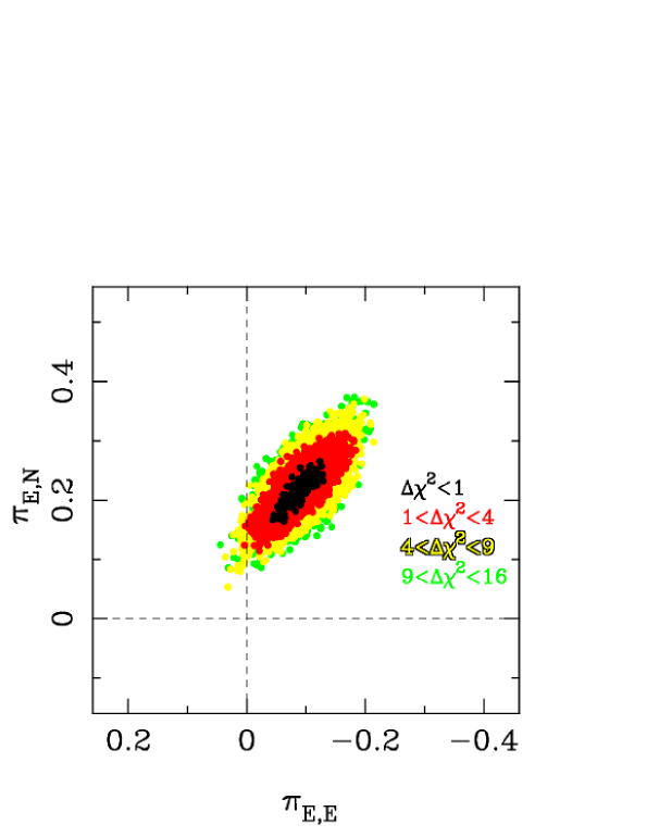
Figure 4: $\Delta\chi^{2}$ map of the parallax parameters of the best fit model with xallarap and parallax effects. The colors of black, red, yellow, green represent $\Delta\chi^{2}=1,4,9,16$, respectively.

In contrast, the probability distribution of the lens properties was also estimated by using the xallarap model parameters in Section 6. We performed fits including both parallax and xallarap effects because parallax amplitude is related to the lens mass. The results are listed in Table 5. The xallarap and parallax model has a binary mass ratio of $q=0.270\pm 0.005$ and a separation of $s=0.083\pm 0.001$ in a unit of Einstein radius with $\xi_{\rm E}=(3.91\pm 0.18)\times 10^{-4}$, and $P_{\xi}=9.139\pm 0.006$ days. Since the orbital period of the source companion is very short, it may be that parallax and xallarap do not affect the same part of the light curve. It is possible that the parallax results are unaffected by xallarap effects. Therefore, the parallax signal has not been detected on the light curve significantly, so we set the upper limit of the parallax amplitude $\pi_{\rm E}<0.5$ from the $\Delta\chi^{2}$ contour map of parallax parameters in Figure 4. This upper limit will imply a lower limit of the lens mass.

4 Source star and the Angular Einstein Radius

The source star angular radius $\theta_{*}$ was determined using source magnitude and color. The source star magnitudes and colors estimated from the light curve fit need to be corrected for extinction and reddening due to the interstellar dust in the line of sight. The Red Clump Giant (RCG) is the standard candle to estimate extinction and reddening. The Color Magnitude Diagram (CMD) was made from CTIO $I$- and $V$- band stars within 2^′ of the source star calibrated to the OGLE-III calalog (Figure 5). In this CMD, we find the RCG centroid to be,

$$(I,V-I)_{\rm clump,obs}=(16.56,3.13)\pm(0.03,0.03).$$ (9)

We adopt the Galactic bulge RCG magnitude $M_{I,RC,0}=-0.10\pm 0.05$ from Nataf (2012) and color $(V-I)_{RC,0}=1.06\pm 0.06$ from Bensby et al. (2011). According to Nishiyama et al. (2005), the clump in this field is 0.1 mag brighter than the Galactic center, which we take to be at $R_{\rm 0}=8.0\pm 0.3$ kpc Yelda et al. (2010). Hence, the distance modulus of the clump is DM=$14.42\pm 0.09$. Thus, the dereddened RCG centroid is expected to be

$$(I,V-I)_{\rm clump,0}=(14.32,1.06)\pm(0.11,0.06).$$ (10)

Comparing these centroids, we find the extinction value $A_{I}$ and reddening value $E(V-I)$ to be, ($A_{I},E(V-I)$) = (2.24, 2.07) $\pm$ (0.11, 0.06).

The source star magnitudes from the light curve fit are $(I,V-I)_{\rm s,obs}=(21.44,2.76)\pm(0.01,0.03)$. Applying $A_{\rm I}$ and $E(V-I)$, the dereddended source color and magnitude $(I,V-I)_{s,0}$ is calculated to be

$$(I,V-I)_{\rm s,0}=(19.20,0.69)\pm(0.11,0.07).$$ (11)

We estimate $(V-K)_{\rm S,0}=1.50\pm 0.18$ magnitude from $(V-I)_{\rm S,0}$ and Bessell & Brett (1988) color-color relation, and so $K=18.40\pm 0.22$. From Kervella et al. (2004), the relationship between color/brightness and a star angular radius is

$$\log(2\theta_{*})=0.0755(V-K)+0.5170-0.2K,$$ (12)

so the source angular radius is

$$\theta_{*}=0.45\pm 0.02\hskip 2.84544pt\mu\mathrm{as}.$$ (13)

Thus, the angular Einstein radius $\theta_{\rm E}$ is calculated by the source angular radius $\theta_{*}$ and $\rho=(2.98\pm 0.04)\times 10^{-4}$ to be

$$\theta_{E}=\frac{\theta_{*}}{\rho}=1.50\pm 0.08\hskip 2.84544pt\mathrm{mas},$$ (14)

and finally the lens-source relative proper motion $\mu_{\rm rel}$ is

$$\mu_{\rm rel}=\frac{\theta_{E}}{t_{\rm E}}=2.70\pm 0.15\hskip 2.84544pt\mathrm{mas}\hskip 2.84544pt\mathrm{yr^{-1}}.$$ (15)

5 Blended Light

Blending magnitudes obtained from the fits are listed in Table 6. The result of the fit indicates that the blending flux in the CTIO $V$-band is $-16.9\pm 8.7$ ADU, however the calculated flux is consistent with zero flux to within 2 sigma. The blending flux in the CTIO $I$-band is also consistent with zero flux to within 2 sigma. Thus, we estimate the upper limit of the brightness by using baseline images from the CTIO $I,V$-band and IRSF $J,H,K_{\rm s}$-band, by taken about 4 years after the peak so that the source star is not magnified by the microlensing. The $I$- and $V$-band magnitude were calibrated to the OGLE-III catalog magnitude, and the $J,H,K_{\rm s}$ band magnitude were calibrated to the 2MASS catalog. The result is that $V>20.90$, and other results are listed in Table 6. These upper limits are estimated from the equation, $M_{\rm limit}=-2.5\log{(5\sqrt{f_{\rm sky}\times\pi r^{2}/G})}+c$, where $f_{\rm sky}$ is sky flux at this target position, $\pi r^{2}$ is a PSF area, $G$ is the gain value, $c$ is the scale factor to calibrate to catalog magnitude. These parameters are listed in Table 7. For $I$-band upper limit on the brightness, we use the results of the modeling in the CTIO data to estimate, $I>19.15$.

6 The Lens Properties

In Section 3 and 4, we obtained the best fit model parameters and the angular Einstein radius from the source brightness. From them, we estimated the lens properties for the two solutions of the parallax model and the xallarap model.

6.1 The parallax model

The both of finite source and parallax effects allow us to determine the physical parameters of the lens properties as the lens total mass $M_{\rm L}$, distance $D_{\rm L}$ and velocity $v$. The lens total mass is described by the angular Einstein radius $\theta_{\rm E}$ and microlens parallax amplitude $\pi_{\rm E}$ as given by

$$M = \frac{\theta_{\rm E}}{\kappa\pi_{\rm E}},$$ (16)

where $\kappa=4G/(c^{2}~{}{\rm AU})=8.144~{}{\rm mas}~{}M_{\odot}^{-1}$. The distance is derived from the Equation 3.

We calculate the lens properties from the parameters of the combined parallax and lens orbital motion model (close separation and $u_{0}<0$). The lens total mass is $M_{\rm L}=1.40\pm 0.18M_{\odot}$, as the components of the lens, the primary lens has $M_{1}=1.06\pm 0.13M_{\odot}$ with a companion $M_{2}=0.34\pm 0.04M_{\odot}$. The distance to the lens is $D_{\rm L}=3.11\pm 0.39~{}\mathrm{kpc}$.

The upper limit of the brightness derives the upper limit of the lens mass. The absolute magnitude $M_{I}$ is calculated by

$$M_{I} = I_{\rm b}-5\log{\frac{D_{\rm L}}{10{\rm pc}}}-A_{I,{\rm L}},$$ (17)

$$= I_{\rm b}-5\log{\frac{D_{\rm L}}{10{\rm pc}}}-A_{I,{\rm S}}+(A_{I,{\rm S}}-A_{I,{\rm L}}),$$ (18)

where $I_{\rm b}$ is the apparent magnitude of the blend, $A_{I,\rm S}$ and $A_{I,\rm L}$ are the extinction toward the source and lens, respectively. Since the lens should be in front of the source, the extinction toward the source is larger than the one of the lens, ($A_{I,\rm S}-A_{I,\rm L})>0$. Therefore, the upper limit of the brightness is $M_{I}>4.4$. Note that this upper limit is quite conservative because there is a possibility that some of the dust is behind the lens. The upper limit of the brightness implies that the upper limit of the lens mass is $M<0.99M_{\odot}$, assuming the primary lens is a main sequence star. The main sequence star is the dominant component in the galaxy, and the upper limit of the lens mass, assuming that the primary lens is a main sequence star, is consistent within the error bars of the primary lens mass calculated by the parallax model parameters. Thus, the parallax model indicates that the binary lens system is likely constructed by the main sequence stars.

6.2 The xallarap model

We also estimated the probability distribution of the lens properties using the combined xallarap and parallax model (close separation and $u_{0}>0$). From the fit parameter for the finite source effects, $\rho$, we were able to calculate the angular Einstein radius. In Section 4, the source angular radius, $\theta_{*}$, and the angular Einstein radius, $\theta_{\rm E}$, are estimated by the combined parallax and lens orbital motion model. On the other hand, for the combined xallarap and parallax model, the $f_{\rm S}\times t_{\rm E}$ were invariant with the different model. Therefore, we can estimate these quantities using the equation (Yee et al., 2009),

$$\theta_{*}=\frac{\sqrt{f_{\rm S}}}{Z},$$ (19)

where $f_{\rm S}$ is the source flux as determined from the model, and $Z$ is the remaining set of factors. The $\theta_{\rm*,xa}$ and $\theta_{\rm E,xa}$ are calculated by the model parameters of $t_{\rm E,xa}=169.4\pm 1.0$ days and $\rho_{\rm xa}=(3.45\pm 0.02)\times 10^{-4}$ that $\theta_{\rm*,xa}=\theta_{*}\times\sqrt{f_{\rm S,xa}/f_{\rm S}}=\theta_{*}\times\sqrt{t_{\rm E}/t_{\rm E,xa}}=0.49\pm 0.03$, and $\theta_{\rm E,xa}=\theta_{\rm*,xa}/\rho_{\rm xa}=1.42\pm 0.10$ mas. Note that the index of “xa” indicates the parameter of the combined xallarap and parallax model. We estimate the probability distribution from Bayesian analysis by combining the Equation 16 and the measured values of $\theta_{\rm E,xa}$ and $t_{\rm E,xa}$.

The mass function adopted for the calculation based on Sumi et al. (2011) Table S3, model #1. The main sequence stars and brown dwarf stars form a power-law function, $dN/dM=M^{-\alpha}$ where $\alpha=2.0$ for ($0.7<M/M_{\odot}<1.0$), $\alpha=1.3$ for ($0.08<M/M_{\odot}<0.7$) and $\alpha=0.5$ for ($0.01<M/M_{\odot}<0.08$). The stellar remnant stars are assumed to be white dwarfs (WDs; $M=0.6M_{\odot},\sigma=0.16$), neutron stars (NSs; $M=1.35M_{\odot},\sigma=0.04$) and black holes (BHs; $M=5M_{\odot},\sigma=1$). These remnants are represented by Gaussians. The fraction of initial numbers of these objects in the four classes MSs (which include main sequence and brown dwarf stars), WDs, NSs and BHs are distributed as 88.8, 10.0, 1.0, and 0.2, respectively. The distance to the Galactic center is assumed to be 8 kpc and the upper limit of microlens parallax amplitude, $\pi_{\rm E}<0.5$, is adopted in the calculation, which affects the lower limit of the lens mass. The upper limit of the brightness, $I_{\rm b,0}=I_{\rm b}-A_{I}>16.91$, is also included.

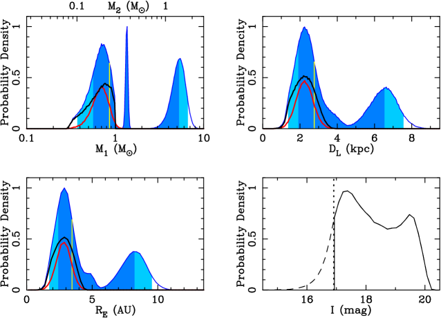
Figure 6: The probability distribution from a Bayesian analysis with the upper limit of lens brightness for mass, $M_{\rm L}$, distance, $D_{\rm L}$, Einstein radius $R_{\rm E}$ and $I$-band magnitude of primary lens brightness. The vertical solid lines in yellow indicate the median values. The distribution described in blue indicates the results with the entire mass function and the curves in black and red represent the results for only main sequence stars and white dwarfs, respectively. The dark and light blue shaded regions indicate the 68% and 95% confidence limits, respectively. In the bottom-right panel, the upper limit of brightness, $I_{\rm b,0}>16.91$ is shown by the vertical dotted line. The dashed curve indicates the rejected area due to the lens brightness constraint. Note that $D_{\rm S}$ is not fixed in the actual Bayesian analysis.

The probability distribution from the Bayesian analysis is shown in Figure 6. The distribution described in blue indicates the results for all mass functions, and the curves in black and red represent the results for only from MSs and WDs, respectively. In the bottom-right panel, the probability distribution for the brightness is derived using only main sequence stars and excludes remnant stars as these should be very faint. The solid and dashed curve indicate the probability of the brightness with and without the upper limit of the brightness $I_{\rm b,0}>16.91$, respectively, and the vertical dashed line represents the upper limit of the brightness. The probability ratio for each class of MSs, WDs, NSs, and BHs is 0.35, 0.23, 0.09, and 0.33, respectively, which indicates that the primary lens is likely a stellar remnant 65% of the time, such as a white dwarf, a neutron star or a black hole.

As a result, the lens properties were derived from the probability distribution as follows: The primary star is a massive star with a mass of $M_{1}=0.9_{-0.3}^{+4.6}M_{\odot}$, distance of $D_{\rm L}=2.6_{-0.9}^{+3.8}$ kpc, and the companion has a mass of $M_{2}=0.2_{-0.1}^{+1.2}M_{\odot}$. The Einstein radius is $R_{\rm E}=3.5_{-1.1}^{+5.2}$ AU, which means that the projected separation is $r_{\perp}=(0.3_{-0.1}^{+0.5},\hskip 5.0pt56_{-18}^{+83})$ AU and the physical three-dimensional separation is $a=(0.4_{-0.2}^{+0.5},\hskip 5.0pt82_{-37}^{+96})$ AU on the close and wide separation model, respectively. The physical three-dimensional separation was estimated by putting a planetary orbit at random inclination, eccentricity and phase (Gould & Loeb, 1992).

Recently, the mass functions of stellar remnants have been updated by improvements of observational methods and detections of stellar remnants (white dwarfs: Kepler et al. (2007), neutron stars: Kiziltan et al. (2010), and black holes: Özel et al. (2010)). However, the qualitative conclusions are not affected by these uncertain mass functions. Thus, we can conclude that the primary lens is most likely to be a stellar remnant such as a white dwarf, a neutron star or a black hole.

7 Discussion and Conclusion

We have reported the binary microlensing event OGLE-2007-BLG-514. This is an extremely high-magnification event ($A>1000$), which enabled follow-up observations of this event. From the binary lens model search, we found that the lens has a stellar binary mass ratio $q\geq 0.1$. The well-known degeneracies of the close/wide separation and impact parameter $u_{0}>0$ and $u_{0}<0$ both remained unresolved in our light-curve analysis. We also search for the higher order effects of microlens parallax, lens orbital motion, and xallarap (source orbital motion) for this event. The xallarap model $\chi^{2}$ is better than the parallax and lens orbital motion model, respectively. However, spurious xallarap signals at this level are common in microlensing (Poindexter et al., 2005). And, the data on this event has high S/N, so we expect that stronger false signals can be caused by systematics. Therefore, the combined parallax and lens orbital motion model is the most plausible solution, but we can not absolutely exclude the xallarap model. Thus, we consider two solutions of the parallax model and xallarap model for the estimation of the lens properties. The best fit model with parallax and lens orbital motion has a binary mass ratio of $q=0.321\pm 0.007$ and a separation of $s=0.072\pm 0.001$ in a unit of Einstein radius with $\pi_{\rm E}=0.13\pm 0.02$. On the other hand, the xallarap and parallax model has a binary mass ratio of $q=0.270\pm 0.005$ and a separation of $s=0.083\pm 0.001$ Einstein radius.

The parallax model parameters allow us to determine the lens properties. According to the model with parallax and lens orbital motion effects, the lens total mass is $M_{\rm L}=1.40\pm 0.18M_{\odot}$, as the components of the lens, the primary lens has $M_{1}=1.06\pm 0.13M_{\odot}$ with a companion $M_{2}=0.34\pm 0.04M_{\odot}$. The distance to the lens is $D_{\rm L}=3.11\pm 0.39~{}\mathrm{kpc}$. The upper limit of the brightness implies that the upper limit of the lens mass is $M<0.99M_{\odot}$, assuming the primary lens is a main sequence star. The main sequence star is the dominant component in the galaxy, and the upper limit of the lens mass, assuming that the primary lens is a main sequence star, is consistent within the error bars of the primary lens mass calculated by the parallax model parameters. Thus, the parallax model indicates that the binary lens system is likely constructed by the main sequence stars.

On the other hand, the probability distribution of the lens properties was estimated by the Bayesian analysis using the xallarap and parallax model. The parallax amplitude, $\pi_{\rm E}<0.5$, is adopted for the upper limit of the lens mass. Also, the upper limit of the brightness in $I$ band was included in the analysis. As a results, the primary star is a massive star with a mass of $M_{1}=0.9_{-0.3}^{+4.6}M_{\odot}$, a distance of $D_{\rm L}=2.6_{-0.9}^{+3.8}$ kpc, and a companion mass of $M_{2}=0.2_{-0.1}^{+1.2}M_{\odot}$. The probability ratio for each class of MSs, WDs, NSs, and BHs is 0.35, 0.23, 0.09, 0.33, respectively, which indicates that the primary lens is likely a stellar remnant 65% of the time, such as a white dwarf, a neutron star or a black hole.

Moreover, based on the OGLE astrometry, we found that the blended light is associated with the event to high precision (the difference of the position of the source and lens is estimated to be 23 mas, i.e., within the astrometric error.). Therefore, we considered three possibilities of where the blended light was coming from. The first is the primary lens. This suggestion is consistent with the parallax model that the primary lens is likely a main sequence star, which has a solar mass. The second is the companion of the lens. This is possible to explain by the results of the xallarap model. For example, if the primary lens is a black hole, the companion of the lens have a mass close to a solar mass. The last is the companion of the source in the xallarap model. But, it is difficult to interpret that the blended light is only coming from the companion of the source because the companion of the source is far from the Earth and very low mass, so the companion is very faint.

As a final conclusion, we found two solutions for this event. The one is the parallax model, which indicates that the binary lens system is likely constructed by the main sequence stars. The another is the xallarap model, which indicates that the primary lens is likely the stellar remnant, such as a white dwarf, a neutron star or a black hole.

In the future, follow-up observations by radio, optical, or X-ray space telescopes will identify whether the primary lens is a main sequence star or a stellar remnant. High spatial resolution observations with large ground-based telescope and Adaptive-Optics instruments, such as the Subaru telescope or the Very Large Telescope (VLT), could estimate more precise brightness from the lens using the source brightness obtained from the modeling. In addition, it has been 4 years since the peak magnification of this event, and the lens-source relative proper motion is $2.70\pm 0.15$ mas year^-1, indicating that the separation of the source and lens on the sky plane is about 10 mas by now. High resolution observation with the space telescope, Hubble Space Telescope (HST), could detect an elongated PSF blended with the lens and source, and verify the nature of the lens.

Microlensing searches are going on throughout the world. In particular, the OGLE group began using a new wide field of view camera, the OGLE-IV (1.4 deg² FOV), in March 2010 and the number of microlensing events dramatically increased after the OGLE-IV upgrade. Of course, the MOA group is continuing to operate its microlensing search with the MOA-II telescope with its wide field of view (2.2 deg²) MOA-cam3 CCD camera (Sako et al., 2008). In 2011, two survey groups found about 1800 microlensing events, which constitutes a two fold increase over last year. More and more binary lens objects varying from planetary systems to massive binary systems can be discovered by further microlensing observation.

Figure 1: The light curve of the binary microlensing event, OGLE-2007-BLG-514. The top panel shows the data points and the best fit model light curve with both parallax and lens orbital motion effects. The residuals between the data points and the model are shown in the bottom panel. Close-up views of two peaks are shown in the corners. Note that the CTIO $H$-band data points have not been shown at the first peak of the light curve for good-looking, but we used in the modeling.

Figure 2: The caustic curve (solid line) plotted for the OGLE-2007-BLG-514 best fit model. The dashed line indicates the source trajectory including both parallax and lens orbital motion effects. The circle on the source trajectory represents the source star size.

Figure 3: The $\Delta\chi^{2}$ of the best xallarap model as a function of the orbital period of the source star and its companion. The dashed and solid lines indicate the model with and without the Kepler constraint, respectively. The cross represents the best fit model with parallax effect.

Figure 5: The $(V-I,I)$ color magnitude diagram of stars within 2^′ of the OGLE-2007-BLG-514 source using $\mu$FUN CTIO data calibrated to the OGLE-III catalog. The triangle and dot indicate the source star and the center of the red clump giant, respectively.

Table 1: Re-normalizing parameters for error bars

data set	$k$	$e_{\rm min}$
OGLE	1.16	0.01
MOA-II	0.85	0.02
$\mu$FUN Auckland	0.93	0.00
$\mu$FUN SMARTS CTIO $V$-band	3.00	0.00
$\mu$FUN SMARTS CTIO $I$-band	1.81	0.00
$\mu$FUN SMARTS CTIO $H$-band	1.00	0.01
$\mu$FUN Campo Catino Austral	0.60	0.00
$\mu$FUN Farm Cove	0.92	0.00
RoboNet Faulkes Telescope North	0.73	0.01
RoboNet Faulkes Telescope South	0.48	0.00
PLANET Canopus	0.72	0.00
IRSF $J$-band	0.76	0.01
IRSF $H$-band	0.83	0.01
IRSF $K_{\rm s}$-band	0.76	0.01

Note. — The formula to re-normalize the error bars is $\sigma^{\prime}_{i}=k\sqrt{\sigma_{i}^{2}+e_{\rm min}^{2}}$, where $\sigma_{i}$ is original error bar of the $i$th data point within a unit of magnitude.

Table 2: Limb darkening coefficients for the source star

filter color	$V$	$R$	$I$	$J$	$H$	$K$
$u$	0.7242	0.6481	0.5618	0.4387	0.3711	0.3212

Note. — These coefficients are for the source star with effective temperature $T_{\rm eff}$=5500 K, surface gravity $\log g$=4.0 cm s^-2 and metallicity $\log$[M/H]=0.3 (Claret, 2000). We used the $R$-band parameter for unfiltered data.

Table 3: Binary lens model parameters for parallax

Model	$t_{0}$	$t_{E}$	$u_{0}$	$q$	$s$	$\alpha$	$\rho$	$\pi_{\rm E,N}$	$\pi_{\rm E,E}$	$\chi^{2}$
	HJD’	[days]	$10^{-3}$			[rad]	$10^{-4}$
close1.+	4386.784	198.96	1.60	0.249	0.0777	0.690	2.93	$\cdots$	$\cdots$	3601.37
$\sigma$	0.001	3.14	0.02	0.007	0.0007	0.002	0.05	$\cdots$	$\cdots$
close1.-	4386.784	199.80	-1.59	0.238	0.0787	5.595	2.91	$\cdots$	$\cdots$	3601.50
$\sigma$	0.001	3.85	0.03	0.009	0.0008	0.002	0.06	$\cdots$	$\cdots$
close2.+	4386.782	254.56	1.27	0.227	0.0709	0.679	2.29	-0.206	0.021	3580.37
$\sigma$	0.001	3.40	0.02	0.007	0.0009	0.002	0.05	0.013	0.006
close2.-	4386.783	205.34	-1.57	0.251	0.0765	5.603	2.85	0.221	0.042	3590.89
$\sigma$	0.001	4.81	0.03	0.008	0.0008	0.002	0.07	0.023	0.010
close3.+	4386.787	200.05	1.58	0.251	0.0773	0.690	2.95	-0.142	-0.642	3593.49
$\sigma$	0.001	2.29	0.02	0.008	0.0009	0.003	0.03	0.203	0.159
close3.-	4386.784	195.45	-1.63	0.241	0.0790	5.599	2.99	-0.079	-0.493	3598.00
$\sigma$	0.001	2.74	0.03	0.005	0.0007	0.003	0.04	0.232	0.250
close4.+	4386.782	246.01	1.31	0.219	0.0729	0.680	2.37	-0.194	0.018	3583.96
$\sigma$	0.001	3.58	0.02	0.009	0.0008	0.002	0.04	0.021	0.008
close4.-	4386.784	198.00	-1.62	0.262	0.0770	5.600	2.96	0.215	0.045	3590.66
$\sigma$	0.001	3.38	0.03	0.009	0.0007	0.002	0.05	0.026	0.010
wide1.+	4386.782	232.96	1.36	0.421	17.3863	0.686	2.51	$\cdots$	$\cdots$	3601.18
$\sigma$	0.001	3.58	0.02	0.016	0.2971	0.002	0.04	$\cdots$	$\cdots$
wide1.-	4386.782	235.81	-1.35	0.450	17.8030	5.596	2.48	$\cdots$	$\cdots$	3601.03
$\sigma$	0.001	4.04	0.02	0.026	0.3277	0.002	0.04	$\cdots$	$\cdots$
wide2.+	4386.781	277.00	1.17	0.395	18.5607	0.677	2.11	-0.174	0.019	3578.93
$\sigma$	0.001	2.77	0.01	0.018	0.2442	0.002	0.02	0.012	0.008
wide2.-	4386.781	238.43	-1.35	0.479	18.1461	5.604	2.45	0.182	0.039	3590.21
$\sigma$	0.001	2.84	0.01	0.018	0.1547	0.003	0.02	0.022	0.006
wide3.+	4386.786	236.20	1.33	0.460	17.9249	0.688	2.49	-0.137	-0.527	3592.68
$\sigma$	0.001	3.16	0.02	0.014	0.1940	0.003	0.03	0.135	0.120
wide3.-	4386.782	237.32	-1.34	0.402	17.3515	5.602	2.47	-0.079	-0.400	3597.90
$\sigma$	0.001	4.11	0.02	0.013	0.1737	0.003	0.05	0.136	0.196
wide4.+	4386.781	264.15	1.22	0.418	18.4004	0.680	2.21	-0.170	0.020	3582.38
$\sigma$	0.001	3.06	0.01	0.011	0.1652	0.002	0.02	0.017	0.006
wide4.-	4386.781	241.60	-1.33	0.477	18.2562	5.605	2.43	0.180	0.035	3590.36
$\sigma$	0.001	3.32	0.02	0.014	0.1797	0.002	0.03	0.019	0.005

Note. — Each model is classified by following characters. The character “1” indicates a binary standard model, the characters “2” and “3” represent models with orbital or terrestrial parallax, respectively. The character “4” indicates a model with both parallax effects. The names, “close” and “wide”, indicate separations $s<1$ and $s>1$, respectively. For the $u_{0}>0$ model, we use the character “+” and for the $u_{0}<0$ model we use the character “-”. The error bars represented as “$\sigma$” are given by MCMC. The $\chi^{2}$ value is the result of the fitting with 3588 data points. Note that the $u_{0}$ conventions are the same as in Figure 2 of (Gould, 2004) and HJD${}^{\prime}\equiv$ HJD - 2,450,000.

Table 4: Binary lens model parameters for lens orbital motion

Model	$t_{0}$	$t_{E}$	$u_{0}$	$q$	$s$	$\alpha$	$\rho$	$\pi_{\rm E,N}$	$\pi_{\rm E,E}$	$\omega$	$ds/dt$	$\chi^{2}$
	HJD’	[days]	$10^{-3}$			[rad]	$10^{-4}$			10-2	10-2
										[rad days-1]	[days-1]
lens orbital motion
close.+	4386.784	170.62	1.94	0.376	0.076	0.647	3.53	$\cdots$	$\cdots$	-4.9390	1.00	3553.26
$\sigma$	0.001	1.60	0.02	0.014	0.001	0.003	0.03	$\cdots$	$\cdots$	0.1753	0.20
close.-	4386.785	178.76	-1.85	0.353	0.075	5.633	3.37	$\cdots$	$\cdots$	4.9103	0.87	3551.59
$\sigma$	0.001	1.91	0.02	0.008	0.001	0.003	0.04	$\cdots$	$\cdots$	0.1955	0.15
wide.+	4386.746	225.95	1.38	0.427	17.552	0.674	2.48	$\cdots$	$\cdots$	-0.0015	-0.57	3601.19
$\sigma$	0.009	3.72	0.03	0.024	0.246	0.010	0.03	$\cdots$	$\cdots$	0.0006	0.16
wide.-	4386.712	215.09	-1.24	0.447	17.874	5.570	2.45	$\cdots$	$\cdots$	0.0070	-0.89	3600.81
$\sigma$	0.006	2.67	0.02	0.015	0.152	0.009	0.02	$\cdots$	$\cdots$	0.0006	0.10
parallax + lens orbital motion
close.+	4386.781	250.29	1.32	0.311	0.066	0.651	2.38	-0.141	-0.010	-3.5485	1.02	3549.82
$\sigma$	0.001	3.42	0.03	0.012	0.001	0.002	0.06	0.012	0.003	0.0051	0.02
close.-	4386.781	202.40	-1.64	0.321	0.072	5.644	2.98	0.131	0.004	4.8568	0.94	3548.29
$\sigma$	0.001	2.28	0.02	0.007	0.001	0.002	0.04	0.015	0.002	0.0035	0.01
wide.+	4386.872	292.38	0.96	0.399	18.358	0.759	2.17	-0.164	0.032	-0.0004	1.42	3583.05
$\sigma$	0.007	3.14	0.02	0.019	0.207	0.006	0.03	0.015	0.007	0.0001	0.08
wide.-	4386.943	288.83	-1.26	0.447	17.936	5.582	2.42	0.180	0.040	-0.0066	1.85	3590.67
$\sigma$	0.004	3.64	0.02	0.019	0.185	0.007	0.03	0.016	0.005	0.0004	0.05

Note. — The names, “close” and “wide”, indicate separations $s<1$ and $s>1$, respectively. For the $u_{0}>0$ model, we use the character “+” and for the $u_{0}<0$ model we use the character “-”. The error bars represented as “$\sigma$” are given by MCMC. The $\chi^{2}$ value is the result of the fitting with 3588 data points. Note that the $u_{0}$ conventions are the same as in Figure 2 of (Gould, 2004) and HJD${}^{\prime}\equiv$ HJD - 2,450,000.

Table 5: Binary lens model parameters for xallarap

Model	$t_{0}$	$t_{E}$	$u_{0}$	$q$	$s$	$\alpha$	$\rho$	$\pi_{\rm E,N}$	$\pi_{\rm E,E}$	$\xi_{\rm E,N}$	$\xi_{\rm E,E}$	RAξ	declξ	Pξ	$\chi^{2}$
	HJD’	[days]	$10^{-3}$			[rad]	$10^{-4}$			$10^{-4}$	$10^{-4}$	[deg]	[deg]	[days]
xallarap
close.+	4386.789	153.18	2.12	0.283	0.0860	0.683	3.83	$\cdots$	$\cdots$	-1.27	4.32	210.6	13.95	9.992	3546.78
$\sigma$	0.001	1.09	0.01	0.006	0.0005	0.004	0.02	$\cdots$	$\cdots$	0.09	0.11	10.1	11.28	0.007
close.-	4386.784	157.59	-2.11	0.291	0.0842	5.616	3.73	$\cdots$	$\cdots$	4.10	3.17	250.4	-63.43	9.992	3547.27
$\sigma$	0.001	1.08	0.02	0.006	0.0005	0.003	0.02	$\cdots$	$\cdots$	0.15	0.18	13.3	9.08	0.011
wide.+	4386.786	187.96	1.74	0.530	16.4576	0.675	3.12	$\cdots$	$\cdots$	-3.67	2.55	203.0	-6.14	9.737	3546.42
$\sigma$	0.001	1.24	0.01	0.014	0.1173	0.003	0.01	$\cdots$	$\cdots$	0.32	0.09	14.2	6.12	0.009
wide.-	4386.786	185.51	-1.75	0.493	16.0743	5.608	3.17	$\cdots$	$\cdots$	2.91	2.74	16.4	1.14	9.366	3544.88
$\sigma$	0.001	1.04	0.01	0.012	0.0994	0.003	0.02	$\cdots$	$\cdots$	0.21	0.13	10.3	7.27	0.006
xallarap + parallax
close.+	4386.788	169.39	1.93	0.270	0.0827	0.677	3.45	0.212	-0.091	-2.66	2.86	247.6	-7.36	9.139	3535.83
$\sigma$	0.001	1.02	0.01	0.005	0.0007	0.003	0.02	0.025	0.015	0.11	0.14	14.1	7.84	0.006
close.-	4386.788	162.58	-2.04	0.264	0.0850	5.608	3.61	0.213	-0.064	6.75	3.93	447.1	-163.07	9.158	3536.47
$\sigma$	0.001	1.36	0.01	0.006	0.0007	0.004	0.03	0.032	0.023	0.15	0.20	15.2	9.75	0.008
wide.+	4386.785	189.06	1.73	0.519	16.4318	0.670	3.10	0.200	-0.096	-1.58	4.41	344.4	5.79	9.347	3537.02
$\sigma$	0.001	1.27	0.01	0.011	0.0779	0.003	0.02	0.024	0.018	0.11	0.15	3.4	5.90	0.003
wide.-	4386.786	193.58	-1.68	0.454	16.0947	5.605	3.04	0.195	-0.084	1.67	4.34	173.2	15.35	9.979	3539.78
$\sigma$	0.001	1.74	0.02	0.010	0.0946	0.003	0.03	0.031	0.018	0.16	0.10	5.4	9.18	0.005

Note. — The names, “close” and “wide”, indicate separations $s<1$ and $s>1$, respectively. For the $u_{0}>0$ model, we use the character “+” and for the $u_{0}<0$ model we use the character “-”. The error bars represented as “$\sigma$” are given by MCMC. The $\chi^{2}$ value is the result of the fitting with 3588 data points. Note that the $u_{0}$ conventions are the same as in Figure 2 of (Gould, 2004) and HJD${}^{\prime}\equiv$ HJD - 2,450,000.

Table 6: Source and Blending brightness

data	$F_{\rm s}$	$F_{\rm s,err}$	$F_{\rm b}$	$F_{\rm b,err}$	Source	error	Blending	error
	[ADU]		[ADU]		Magnitude		Magnitude
OGLE $I$	12.63	0.10	62.4	3.0	21.25	0.01	19.51	0.04
CTIO $V$	0.83	0.02	-16.9	8.7	24.20	0.03	$\cdots$	$\cdots$
CTIO $I$	10.58	0.13	50.3	27.9	21.44	0.01	19.75	0.60
CTIO $H$	103.16	1.95	2012	402	18.97	0.02	15.74	0.22
IRSF $J$	58.37	0.30	103	128	19.59	0.01	18.97	1.35
IRSF $H$	113.28	0.51	382	211	18.87	0.01	17.54	0.60
IRSF $K_{\rm s}$	146.48	0.69	1301	294	18.59	0.01	16.21	0.25

Note. — The photometry file for each data set excluding the OGLE data was made by the DoPHOT tool to estimate blending fluxes and source fluxes.

Table 7: The upper limit of the lens brightness

data	$f_{\rm sky}$	$r$	$G$	$c$	Mlimit	Mlimit,blend
	[ADU]	[pixel]	[$e^{-}$/ADU]
OGLE $I$	$\cdots$	$\cdots$	$\cdots$	$\cdots$	$\cdots$	19.47
CTIO $V$	379.2	5	2.3	27.87$\pm$0.08	20.90	$\cdots$
CTIO $I$	609.4	5	2.3	26.91$\pm$0.18	19.59	19.15
IRSF $J$	1297.7	4	5.0	24.32$\pm$0.09	17.33	17.62
IRSF $H$	5427.7	4	5.0	24.35$\pm$0.08	16.61	16.96
IRSF $K_{\rm s}$	5955.6	3	5.0	23.50$\pm$0.08	15.97	15.96

Note. — The $f_{\rm sky}$ is sky flux at this target position, $r$ is the radius of a PSF area, and $c$ is the scale factor to calibrate to catalog magnitude. M_limit and M_limit,blend indicate the upper limit of the lens brightness estimated by the flux in the images observed in 2011 and the blending magnitude obtained from the fit, respectively.

References

- Abe et al. (2003) Abe, F., et al. 2003, A&A, 411, L493
- Agol et al. (2002) Agol, E., Kamionkowski, M, Koopmans, L. V. E., & Blandford, R. D. 2002, ApJ, 576, L131
- Albrow et al. (1998) Albrow, M., et al. 1998, ApJ, 509, 687
- Albrow et al. (2009) Albrow, M. D., et al. 2009, MNRAS, 397, 2099
- An et al. (2002) An, J. H., Albrow, M. D., Beaulieu, J.-P., et al. 2002, ApJ, 572, 521
- Batista et al. (2011) Batista, V. 2011, A&A, 529, A102
- Bennett (2010) Bennett, D. P. 2010, ApJ, 716, 1408
- Bennett et al. (2002) Bennett, D. P., et al. 2002, ApJ, 579, 639
- Bennett et al. (2008) Bennett, D. P., et al. 2008, ApJ, 684, 663
- Bensby et al. (2010) Bensby, T., et al. 2010, A&A, 512, A41
- Bensby et al. (2011) Bensby, T., et al. 2011, A&A, 533, A134
- Bessell & Brett (1988) Bessell, M., S., & Brett, J. M. 1988, PASP, 100, 1134
- Bond et al. (2001) Bond, I.A., et al. 2001, MNRAS, 327, 868
- Bramich (2008) Bramich, D. M. 2008, MNRAS, 386, L77
- Claret (2000) Claret, A. 2000, A&A, 363, 1081
- Dominik (1999) Dominik, M. 1999, A&A, 349, 108
- Doran & Müller (2004) Doran, M., & Müller, C. M. 2004, J. Cosmology Astropart. Phys, 9, 3
- Epstein et al. (2010) Epstein, C. R., Johnson. J. A., Dong. S., Udalski, A., Gould. A., & Becker, G. 2010, ApJ, 709, 447
- Gould & Loeb (1992) Gould, A., & Loeb, A. 1992, ApJ, 396, 104
- Gould (2000) Gould, A. 2000, ApJ, 542, 785
- Gould (2004) Gould, A. 2004, ApJ, 606, 319
- Gould et al. (2010) Gould, A., et al. 2010, ApJ, 720, 1073
- Han & Gould (2003) Han, C., Gould, A. 2003, ApJ, 592, 172
- Han & Hwang (2009) Han, C., & Hwang, K.-H. 2009, ApJ, 707, 1264
- Hwang et al. (2011) Hwang, K.-H., et al. 2011, MNRAS, 413, 1244
- Kepler et al. (2007) Kepler, S. O., Kleinman, S. J., Nitta, A., Koester, D., Castanheira, B. G., Giovannini, O., Costa, A. F. M., & Althaus, L. 2007, MNRAS, 375, 1315
- Kervella et al. (2004) Kervella, P., Thévenin, F., Di Folco, E., & Ségransan, D. 2004, A&A, 426, 297
- Kiziltan et al. (2010) Kiziltan, B., Kottas, A., & Thorsett, S. E. 2010, submitted to the ApJ, arXiv:1011.4291
- Mao et al. (2002) Mao, S., et al. 2002, MNRAS, 329, 349
- Nataf (2012) Nataf, D. 2012, in preparation
- Nishiyama et al. (2005) Nishiyama, S., et al. 2005, ApJ, 621, L105
- Özel et al. (2010) Özel, F., Psaltis, D., Narayan, R., & McClintock, J. E. 2010, ApJ, 725, 1918
- Poindexter et al. (2005) Poindexter, S., Afonso, C., Bennett, D. P., Glicenstein, J-F., Gould, A., Szymanśki, M, K., & Udalski, A. 2005, ApJ, 633, 914
- Rattenbury et al. (2005) Rattenbury, N. J., et al. 2005, A&A, 439, 645
- Sako et al. (2008) Sako, T., et al. 2008, Exp. Astron., 22, 51
- Schechter et al. (1993) Schechter, P. L., Mateo, M., Saha, A. 1993, PASP, 105, 1342
- Shin et al. (2011) Shin, I.-G., et al. 2011, ApJ, 735, 85
- Shin et al. (2012) Shin, I.-G., et al. 2012, ApJ, 746, 127
- Skowron et al. (2011) Skowron, J., et al. 2011, ApJ, 738, 87
- Sumi et al. (2010) Sumi, T., et al. 2010, ApJ, 710, 1641
- Sumi et al. (2011) Sumi, T., et al. 2011, Nature, 473, 349
- Tsapras et al. (2009) Tsapras, Y., et al. 2009, Astron. Nachr. , 330, 4
- Udalski et al. (1994) Udalski, A., et al. 1994, ApJ, 436, L103
- Udalski (2003) Udalski, A. 2003, Acta Astron., 53, 291
- Verde et al. (2003) Verde, L., et al. 2003, ApJ, 148, 195
- Yee et al. (2009) Yee, J. C., et al. 2009, ApJ, 703, 2082
- Yelda et al. (2010) Yelda, S., Ghez, A. M., Lu, J. R., Do, T., Clarkson, W., & Matthews, K. 2011, in ASP Conf. Ser. 439, The Galactic Center: A Window to the Nuclear Environment of Disk Galaxies, ed. M. R. Morris, Q. D. Wang, & F. Yuan (San Francisco, CA: ASP), 167
- Yoo et al. (2004) Yoo, J., et al. 2004, ApJ, 603, 139