Joint numerical ranges, quantum maps,
and joint numerical shadows

Abstract

We associate with a $k$-tuple of hermitian $N\times N$ matrices a probability measure on $\mathbb{R}^{k}$ supported on their joint numerical range: The joint numerical shadow of these matrices. When $k=2$ we recover the numerical range and the numerical shadow of the complex matrix corresponding to a pair of hermitian matrices. We apply this material to the theory of quantum information. Thus, we show that quantum maps on the set of quantum states defined by Kraus operators satisfying the identity resolution assumption shrink joint numerical ranges.

1 Introduction

Let ${\mathcal{H}}_{N}$ be the $N$-dimensional Hilbert space with the scalar product $\langle\varphi|\psi\rangle$, and let $A$ be an operator on ${\mathcal{H}}_{N}$. Its numerical range (also called the field of values) $W(A)\subset\mathbb{C}$ is the set of numbers $z=\langle\psi|A|\psi\rangle$, where $\langle\psi|\psi\rangle=1$ [1, 2]. A crucial fact, conjectured by O. Toeplitz in 1918 and proved by F. Hausdorff in 1919 [3, 4] is that $W(A)$ is convex. See [5] for an exposition of [3, 4] from a modern perspective. If $A$ is a normal operator, then $W(A)$ is the convex hull of the spectrum of $A$, hence a convex polygon. For generic $A$ the boundary $\partial W(A)$ is smooth [6]. If $N=2$, $\partial W(A)$ is a (possibly degenerate) ellipse [3, 7]. See [8] for $W(A)$ when $N=3$.

The present work is motivated by the applications of numerical range and related material in quantum mechanics, especially in the theory of quantum information [9, 10, 11]. We will freely use the relevant physics terminology in what follows. The set $\Omega_{N}$ of pure quantum states is naturally isomorphic to the complex projective space ${\mathbb{C}}P^{N-1}$. Quantum states are the operators $\rho\geq 0$ on ${\mathcal{H}}_{N}$ satisfying Tr$\rho=1$. The set ${\mathcal{Q}}_{N}$ of quantum states is convex, and $\Omega_{N}\subset{\mathcal{Q}}_{N}$ is the set of extremal points of ${\mathcal{Q}}_{N}$. The elements of ${\mathcal{Q}}_{N}\setminus\Omega_{N}$ are mixed quantum states.

For applications to quantum information it is crucial that $W(A)$ is a plane projection of $\Omega_{N}$ [12]. If $N=2$ (i.e., the one qubit case), $\Omega_{2}={\mathbb{C}}P^{1}$ is the Bloch sphere and ${\mathcal{Q}}_{2}\subset{\mathbf{R}}^{3}$ is the Bloch ball. The fact that a projection of the two-sphere is a (possibly degenerate) ellipse underlies the well known claims about numerical ranges of $2\times 2$ matrices [7]. The numerical shadow of an operator $A$ on ${\mathcal{H}}_{N}$ is a probability distribution $P_{A}(z)$ supported on $W(A)$ [15, 13, 14]. Let $|\psi\rangle$ be distributed on the unit sphere $S({\mathcal{H}}_{N})$ according to the Haar measure. Then $P_{A}(z)$ is the probability density of $z=\langle\psi|A|\psi\rangle$. In the one qubit case, $P_{A}(z)$ is the density of the plane shadow of the Bloch sphere under a light beam  [15].

Let $A_{1},\dots A_{m}$ be hermitian operators on $\mathcal{H}_{N}$. Their joint numerical range (JNR) [17] is the set in $\mathbb{R}^{m}$ defined by

$$W(A_{1},\dots,A_{m})\;=\;\{(\langle\psi|A_{1}|\psi\rangle,\dots,\langle\psi|A_{m}|\psi\rangle\,):\langle\psi|\psi\rangle=1\}.$$ (1)

Since $W(A_{1},A_{2})=W(A_{1}+iA_{2})$, equation  (1) generalizes the notion of the numerical range of a complex operator. We note that $W(A_{1},\dots,A_{m})$ is not necessarily convex for $m>2$ [17]. For instance, the JNR of Pauli matrices is the Bloch sphere; see section  2.

We study the above notions and the relationships between them and quantum maps. Theorem  1 in section  2 shows that the JNR of an $m$-tuple of hermitian operators is a linear projection of the set of pure quantum states to $\mathbb{R}^{m}$. In section  4 we associate with any $m$-tuple of hermitian operators a probability measure on ${\mathbf{R}}^{m}$. This is the joint numerical shadow of the $m$-tuple of hermitian operators; it extends the concept of numerical shadow of a complex operator  [15, 13, 14, 16]. We point out a few basic properties of joint numerical shadows, deferring a deeper study to a separate publication.

Let $\Phi$ be the quantum map on the set of quantum states defined by a $k$-tuple of Kraus operators satisfying the identity resolution  (13). In section  3 we study the effects of $\Phi$ on $m$-tuples of hermitian operators. As Corollaries  3 and  4 show, $\Phi$ shrinks the joint numerical ranges.

Throughout the paper we emphasize the applications of our material in the theory of quantum information. Examples 1, 2, 3, 4, 5 and 6 illustrate these applications. For instance, examples 3 and 4 show the shrinking of numerical ranges under particularly well known quantum maps in the qubit and the qutrit cases.

2 Joint numerical ranges

Let $\mathcal{L}_{N}$ (resp. $\mathcal{M}_{N}$, $\mathcal{P}_{N}$, $\mathcal{Q}_{N}$) denote the space of all (resp. hermitian, positive definite, positive definite with trace $1$) linear operators on ${\mathcal{H}}_{N}$. Let $\Omega_{N}\subset\mathcal{Q}_{N}$ be the set of rank one projections. As vector spaces, $\mathcal{L}_{N}=\mathbb{C}^{N^{2}},\mathcal{M}_{N}=\mathbb{R}^{N^{2}}$. The scalar product

$$(A,B)=\rm{tr}(AB^{*}),$$ (2)

makes $\mathcal{L}_{N}$ (resp. $\mathcal{M}_{N}\subset\mathcal{L}_{N}$) a Hilbert space (resp. Euclidean space). The set $\mathcal{P}_{N}\subset\mathcal{M}_{N}$ is a closed convex cone. Its interior consists of strictly positive operators, $\rho>0$, and its apex is the zero operator. The set $\mathcal{Q}_{N}$ is the intersection of $\mathcal{P}_{N}$ and the hyperplane $\{\rm{Tr}\rho=1\}$. It is a bounded convex region (i.e., has nonempty interior) in the $(N^{2}-1)$-dimensional affine space, and $\Omega_{N}\subset\mathcal{Q}_{N}$ is the set of its extremal points. For a unit vector $\psi\in\mathcal{H}_{N}$ we set $\rho_{\psi}=|\psi\rangle\langle\psi|\in\Omega_{N}$. The manifold $\mathbb{C}P^{N-1}$ is the quotient of the unit sphere $S(\mathcal{H}_{N})$ by the natural linear action of the unit circle $S^{1}\subset\mathbb{C}$. The map $\psi\mapsto\rho_{\psi}$ yields an isomorphism of $\mathbb{C}P^{N-1}$ and $\Omega_{N}$. In what follows we will identify $\mathbb{C}P^{N-1}$ and $\Omega_{N}$ via this isomorphism.

Let $A_{1},\dots,A_{m}\in\mathcal{M}_{N}$ be arbitrary. The mapping from $\mathbb{C}P^{N-1}$ to $\mathbb{R}^{m}$ given by

$${\rm jnr}_{(A_{1},\dots,A_{m})}:|\psi\rangle\mapsto(\langle\psi|A_{1}|\psi\rangle,\dots,\langle\psi|A_{m}|\psi\rangle).$$ (3)

is the joint numerical range map. The range $W(A_{1},\dots,A_{m})$ of this map is the joint numerical range (JNR) of operators $A_{1},\dots,A_{m}$. By the isomorphism $\mathbb{C}P^{N-1}\simeq\Omega_{N}$, we have ${\rm jnr}_{(A_{1},\dots,A_{m})}:\Omega_{N}\to\mathbb{R}^{m}$.

We will recall a few basic notions in affine geometry. By a vector space we will mean a finite dimensional real vector space. Let $V$ be a vector space. A set $H\subset V$ is an affine subspace if there is a linear subspace $H_{0}\subset V$ and a vector $h_{0}\in H$ such that $H=H_{0}+h_{0}$. Let $G\subset U,H\subset V$ be affine subspaces. Let $G_{0}\subset U,H_{0}\subset V$ be the corresponding linear subspaces. A map $Af:G\to H$ is an affine isomorphism if there is a linear isomorphism $Af_{0}:G_{0}\to H_{0}$ and vectors $h_{0}\in H,g_{0}\in G$ so that

$$Af(g)=Af_{0}(g-g_{0})+h_{0}.$$

Definition 1

Let $U,V$ be vector spaces, and let $X\subset U,Y\subset V$ be arbitrary sets. They are affinely isomorphic if there exist affine subspaces $H\subset U,G\subset V$ such that $X\subset G,Y\subset H$, and an affine isomorphism $A:G\to H$ such that $A(X)=Y$. The induced map $A:X\to Y$ is an affine isomorphism of $X$ onto $Y$.

Note that linear isomorphism of sets are the special cases in the above setting when the subspaces and the maps in question are, actually, linear. We will not distinguish between the linear and affine situations in what follows.

We will now expose a general topic in linear algebra. Let $U,V$ be vector spaces. We assume that $U$ is a Euclidean space with the scalar product $(\cdot,\cdot)$. Let $m\geq 1$. With any nonzero vectors $u_{1},\dots,u_{m}\in U$ and $v_{1},\dots,v_{m}\in V$ we associate a linear operator $L:U\to V$ by

$$L(u)=\sum_{i=1}^{m}(u,u_{i})v_{i}.$$ (4)

Let $\mathcal{A}\subset U$ (resp. $\mathcal{B}\subset V$) be the subspace spanned by $u_{1},\dots,u_{m}$ (resp. $v_{1},\dots,v_{m}$). We will need a simple lemma about the operator in equation  (4).

Lemma 1

1. Let $\dim\mathcal{A}=p\leq m$. Assume without loss of generality that the vectors $u_{1},\dots,u_{p}$ span $\mathcal{A}$. Then there are vectors $\tilde{v}_{1},\dots,\tilde{v}_{p}\in\mathcal{B}$ such that the linear operator in equation  (4) satisfies

$$L(u)=\sum_{i=1}^{p}(u,u_{i})\tilde{v}_{i}.$$ (5)

2. Let $\dim\mathcal{B}=q\leq m$. Assume without loss of generality that the vectors $v_{1},\dots,v_{q}$ span $\mathcal{B}$. Then there are vectors $\tilde{u}_{1},\dots,\tilde{u}_{q}\in\mathcal{A}$ such that the linear operator in equation  (4) satisfies

$$L(u)=\sum_{i=1}^{q}(u,\tilde{u}_{i})v_{i}.$$ (6)

3. If $p=m$ (resp. $q=m$) then $\tilde{v}_{i}=v_{i}$ (resp. $\tilde{u}_{i}=u_{i}$) for $1\leq i\leq m$.

The proposition below is immediate from Lemma  1.

Proposition 1

Let the setting be as in Lemma  1, and let $Pr_{\mathcal{A}}:U\to\mathcal{A}$ be the orthogonal projection. Then i) There is a unique linear operator $M:\mathcal{A}\to\mathcal{B}$ such that $L=M\circ Pr_{\mathcal{A}}$; ii) If $\dim\mathcal{A}=m$ (resp. $\dim\mathcal{B}=m$) then $M$ is surjective (resp. injective); iii) If $\dim\mathcal{A}=\dim\mathcal{B}=m$ then $M$ is an isomorphism.

Let $G,H\subset U$ be affine subspaces in a vector space. We say that they are parallel if $H=G+u_{0}$ for some $u_{0}\in U$.

Corollary 1

Let $U,V$ be vector spaces, and let $L:U\to V$ be as in equation  (4). Let $\mathcal{A}\subset U,\mathcal{B}\subset V$ be the subspaces spanned by the vectors $u_{1},\dots,u_{m}$ and $v_{1},\dots,v_{m}$ respectively. Let $M:\mathcal{A}\to\mathcal{B}$ be the operator from Proposition  1.

Let $G\subset U$ be an affine subspace containing a subspace parallel to $\mathcal{A}$. Let $\Gamma\subset G$ be an arbitrary set. If $M$ is injective, then $Pr_{\mathcal{A}}(\Gamma)$ and $L(\Gamma)$ are affinely isomorphic.

Proof. Let $u_{0}\in U$ be such that $\mathcal{A}=G+u_{0}$. Let $\mathcal{B}_{0}\subset\mathcal{B}$ be the range of $M$. Thus, $M:\mathcal{A}\to\mathcal{B}_{0}$ is a linear isomorphism. By Proposition  1, we have

$$L(\Gamma+u_{0})=M\,Pr_{\mathcal{A}}(\Gamma+u_{0})=M(\Gamma+u_{0})\subset\mathcal{B}_{0}.$$

The mapping $u\mapsto L(u+u_{0})$ induces an affine isomorphism of $G$ and $\mathcal{B}_{0}$.   

We will now apply the above material to joint numerical ranges.

Theorem 1

Let $A_{1},\dots,A_{m}\in\mathcal{M}_{N}$ be traceless, linearly independent hermitian operators. Let $\mathcal{A}\subset\mathcal{M}_{N}$ be the subspace spanned by them. Then i) The joint numerical range of $A_{1},\dots,A_{m}$ is affinely isomorphic to $Pr_{\mathcal{A}}(\Omega_{N})$; ii) The convex hull of the joint numerical range of $A_{1},\dots,A_{m}$ is affinely isomorphic to $Pr_{\mathcal{A}}(\mathcal{Q}_{N})$.

Proof. Let $U=\mathcal{M}_{N},V=\mathbb{R}^{m}$. Let $v_{1},\dots,v_{m}$ be the standard basis in $\mathbb{R}^{m}$. Then the map $jnr_{A_{1},\dots,A_{m}}$ has the form equation  (4) with $u_{i}=A_{i}$. By Proposition  1, the map $M:\mathcal{A}\to\mathbb{R}^{m}$ is a linear isomorphism. Set $G=\{X\in\mathcal{M}_{N}:\rm{tr}(X)=1\}$. Then $G\subset\mathcal{M}_{N}$ is an affine hyperplane containing the affine subspace $\mathcal{A}+\mathbf{1}_{N}$. Claim i) now follows from Corollary  1.

The convex hulls of affinely isomorphic sets are affinely isomorphic. Hence, claim i) implies claim ii).   

Corollary 2

Let the setting be as in Theorem  1, with $m=N^{2}-1$. Then $W(A_{1},\dots,A_{m})$ is affinely isomorphic to $\Omega_{N}$ and $\rm conv[W(A_{1},\dots,A_{m})]$ is affinely isomorphic to $\mathcal{Q}_{N}$.

Proof. This is a special case of Theorem  1. In this case the affine hyperplane $G$ is parallel to $\mathcal{A}$. Hence $Pr_{\mathcal{A}}$ induces an affine isomorphism of $\Omega_{N}$ and $Pr_{\mathcal{A}}(\Omega_{N})$.   

Example 1. Let $N=2$. The Pauli matrices

$$\sigma_{1}=\left[\begin{array}[]{cc}0&1\\ 1&0\end{array}\right],\ \ \sigma_{2}=\left[\begin{array}[]{cc}0&-i\\ i&0\end{array}\right],\ \ \sigma_{3}=\left[\begin{array}[]{cc}1&0\\ 0&-1\end{array}\right]$$ (7)

form an orthogonal basis in the space of traceless Hermitian $2\times 2$ matrices. By Corollary  2, $W(\sigma_{1},\sigma_{2},\sigma_{3})\subset\mathbb{R}^{3}$ is the unit sphere. Indeed, this also holds by an elementary computation. Let $\psi=[z_{1},z_{2}]$. Denote by $F:\mathbb{C}^{2}\to\mathbb{R}^{3}$ the joint numerical range map; (see equation  (3)). Then

$$F(\psi)=[z_{1}\bar{z}_{2}+z_{2}\bar{z}_{1},i(z_{1}\bar{z}_{2}-z_{2}\bar{z}_{1}),z_{1}\bar{z}_{1}+z_{2}\bar{z}_{2}],$$

and the sum of squared coordinates is $(|z_{1}|^{2}+|z_{2}|^{2})^{2}$.

Let $\rho$ be a $2\times 2$ density matrix. Its Bloch vector $(\tau_{1},\tau_{2},\tau_{3})=\tau\in{\mathbf{R}}^{3}$ is defined by the decomposition

$$\rho=\frac{1}{2}{\mathbf{1}}_{2}+\sum_{j=1}^{3}\tau_{j}\sigma_{j}$$ (8)

where $\tau_{j}=\rm{tr}(\sigma_{j}\rho)/2$. Since $\rho=\rho^{*}$, we have $\tau\in{\mathbf{R}}^{3}$, and since $\rho\geq 0$

$$\sqrt{\tau_{1}^{2}+\tau_{2}^{2}+\tau_{3}^{2}}=||\tau||\leq 1/2.$$

The equality $||\tau||=1/2$ holds if and only if $\rho$ is a pure state. Thus, the map ${\rm jnr}_{(\sigma_{1},\sigma_{2},\sigma_{3})}$ yields an isomorphism of $\mathcal{Q}_{2}$ (resp. $\Omega_{2}$) and the Bloch ball (resp. Bloch sphere).

Example 1 generalizes to $N>2$ as follows. Denote by $d=N^{2}-1$ the dimension of the space of traceles $N\times N$ hermitian matrices with the scalar product  (2). Let $\lambda_{1},\dots,\lambda_{d}$ be an orthogonal, but not necessarily an orthonormal, basis. For instance, for $N=3$ the Gell–Mann matrices $(\lambda_{1},\dots,\lambda_{8})$ satisfy the orthogonality relations $\rm{tr}(\lambda_{j}\lambda_{k})=2\delta_{jk}$ [19]. Let $\rho$ be a $N\times N$ state. The counterpart of equation  (8) is

$$\rho=\frac{1}{N}{\mathbf{1}}_{N}+\sum_{j=1}^{d}\tau_{j}\lambda_{j}.$$ (9)

The generalized Bloch vector $\tau=\tau(\rho)$ has $d$ components $\tau_{j}={\rm Tr}(\rho\lambda_{j})/{\rm Tr}(\lambda_{j}^{2})$. If the basis $\lambda_{1},\dots,\lambda_{d}$ is orthonormal and $\rho_{\psi}=|\psi\rangle\langle\psi|$ is a pure state, then $\tau_{\psi}=\tau(\rho_{\psi})$ satisfies $\tau_{j}=\langle\psi|\lambda_{j}|\psi\rangle$. Hence $\tau_{\psi}\in W(\lambda_{1},\dots\lambda_{d})$.

By Corollary  2, the convex hull $\rm conv[W(\lambda_{1},\dots\lambda_{d})]$ is affinely isomorphic to the set $\mathcal{Q}_{N}$ of quantum states. By Theorem 1, if $\lambda_{1},\dots,\lambda_{m}$ are linearly independent, then the joint numerical range $W(\lambda_{1},\dots,\lambda_{m})$ is affinely isomorphic to a projection of $\mathcal{Q}_{N}$ to ${\mathbf{R}}^{m}$. Compare with the results in  [17, 12].

3 Quantum maps

We recall that the set $\mathcal{L}_{N}$ of operators on ${\mathcal{H}}_{N}$ is a Hilbert space with the scalar product given by equation  (2). Let $\mathcal{L}\mathcal{L}_{N}$ be the space of linear operators on $\mathcal{L}_{N}$. For $\Phi\in\mathcal{L}\mathcal{L}_{N}$ we denote by $\Phi^{*}\in\mathcal{L}\mathcal{L}_{N}$ its adjoint. For $X,Y\in\mathcal{L}_{N}$ we define $\Phi_{X|Y}\in\mathcal{L}\mathcal{L}_{N}$ by

$$\Phi_{X|Y}(A)=XAY^{*}.$$ (10)

Let $X_{1},\dots,X_{k}\in\mathcal{L}_{N}$ be arbitrary. We set

$$\Phi_{(X_{1},\dots,X_{k})}=\sum_{i=1}^{k}\Phi_{X_{i}|X_{i}}.$$ (11)

We will often use the notation $\Phi=\Phi_{(X_{1},\dots,X_{k})}$. In the physics literature the transformations of $\mathcal{P}_{N}$ defined by

$$\rho_{1}=\Phi(\rho)=\sum_{i=1}^{k}X_{i}\rho X_{i}^{*}.$$ (12)

are called quantum maps. They correspond to generalized quantum measurements with $k$ possible outcomes [18]. Operators $X_{i}\in\mathcal{L}_{N}$ are the measurement operators or Kraus operators. Let $\Phi=\Phi_{(X_{1},\dots,X_{k})}$. Then $\Phi_{(X_{1}^{*},\dots,X_{k}^{*})}=\Phi^{*}$, the adjoint operator with respect to the scalar product  (2). In the physics literature the quantum map $\Phi^{*}$ is dual to $\Phi$. The duality of quantum maps corresponds to the duality between the Schrödinger and the Heisenberg representations in quantum mechanics. In the former, the quantum states $\rho\in\mathcal{P}_{N}$ evolve via $\rho_{1}=\Phi(\rho)$, while the observables $A\in\mathcal{M}_{N}$ do not. In the latter, the quantum states do not change and the observables evolve by $A\mapsto A_{1}=\Phi^{*}(A)$.

We will now establish a few basic properties of quantum maps. The following lemma, whose proof is left to the reader, will be used in Proposition  1.

Lemma 2

1. The operators $\Phi_{X|Y}$ span the vector space $\mathcal{L}\mathcal{L}_{N}$.

2. Let $X_{1},Y_{1},X_{2},Y_{2}\in\mathcal{L}_{N}$. Then

$$\Phi_{X_{2}|Y_{2}}\Phi_{X_{1}|Y_{1}}=\Phi_{X_{2}X_{1}|Y_{2}Y_{1}}.$$

3. We have

$$\left(\Phi_{X|Y}\right)^{*}=\Phi_{X^{*}|Y^{*}}.$$

Definition 2

We will denote by $\mathbf{1}\in\mathcal{L}_{N}$ the identity operator. Let $k\geq 1$. We say that the $k$-tuple of operators $X_{1},\dots,X_{k}\in\mathcal{L}_{N}$ is an identity resolution if

$$\sum_{i=1}^{k}X_{i}X_{i}^{*}=\mathbf{1}.$$ (13)

The dual property

$$\sum_{i=1}^{k}X_{i}^{*}X_{i}=\mathbf{1},$$ (14)

holds if and only if $X_{1}^{*},\dots,X_{k}^{*}$ is an identity resolution.

Proposition 1

Let $X_{1},\dots,X_{k}\in\mathcal{L}_{N}$ be arbitrary, and let $\Phi=\Phi_{(X_{1},\dots,X_{k})}\in\mathcal{L}\mathcal{L}_{N}$. Then the following holds.

1. The quantum map $\Phi:\mathcal{L}_{N}\to\mathcal{L}_{N}$ preserves $\mathcal{M}_{N}$ and $\mathcal{P}_{N}$.

2. The operators $X_{1},\dots,X_{k}$ satisfy equation  (13) if and only if $\Phi:\mathcal{L}_{N}\to\mathcal{L}_{N}$ preserves $\mathbf{1}$.

3. The operators $X_{1},\dots,X_{k}$ satisfy equation  (14) if and only if i) the map $\Phi$ preserves the trace; ii) the map $\Phi^{*}$ preserves $\mathbf{1}$.

4. If $X_{1},\dots,X_{k}$ satisfy equation  (14), then $\Phi$ preserves $\mathcal{Q}_{N}$.

Proof. It suffices to prove 1) for operators $\Phi=\Phi_{X|X}$. The former property is immediate from $(XAX^{*})^{*}=XA^{*}X^{*}$, and the latter from $\langle XAX^{*}v,v\rangle=\langle AX^{*}v,X^{*}v\rangle$. Claim 2) is immediate from the definition of $\Phi$. We have

$$\rm{Tr}\left(\Phi(A)\right)=(\Phi(A),\mathbf{1})=(A,\Phi^{*}(\mathbf{1})).$$

Claim 3) now follows from Lemma  2. Claim 4) is immediate from 1) and 3).   

Set $\Phi=\Phi_{(X_{1},\dots,X_{k})}$. We say that the quantum map $\Phi$ is unital (resp. trace preserving) if $\Phi(\mathbf{1})=\mathbf{1}$ (resp. $\rm{Tr}\left(\rho(\Phi)\right)=\rm{Tr}\Phi$). By Proposition  1, a quantum map is unital (resp. trace preserving) if and only if equation  (13) (resp. equation  (14)) is satisfied. Since

$${\rm Tr}\left(\Phi(\rho)A\right)={\rm Tr}\left(\sum_{i}X_{i}\rho X_{i}^{*}A\right)={\rm Tr}\left(\sum_{i}\rho X_{i}^{*}AX_{i}\right)={\rm Tr}\left(\rho\Phi^{*}(A)\right),$$

$\Phi$ is trace preserving (resp. unital) if and only if $\Phi^{*}$ is unital (resp. trace preserving).

For $\psi\in\mathcal{H}_{N}$ we set $\rho_{\psi}=|\psi\rangle\langle\psi|$. Then $\rho_{\psi}\in\mathcal{P}_{N}$, and for any $a\in\mathbb{C}$ we have

$$\rho_{a\psi}=|a|^{2}\rho_{\psi}.$$ (15)

In particular, $\rho_{\psi}=0$ if and only if $\psi=0$ and $\rho_{\psi}\in\mathcal{Q}_{N}$ if and only if $||\psi||=1$.

Proposition 2

Let $X_{1},\dots,X_{k}\in\mathcal{L}_{N}$, and let $\Phi=\Phi_{(X_{1},\dots,X_{k})}$. Let $\psi\in\mathcal{H}_{N}$ be any vector. For $1\leq i\leq k$ such that $X_{i}\psi\neq 0$, set $\psi_{i}=X_{i}\psi/||X_{i}\psi||$.

Then

$$\Phi(\rho_{\psi})=\sum_{i}||X_{i}\psi||^{2}\rho_{\psi_{i}}.$$ (16)

Proof. Let $X,Y\in\mathcal{L}_{N}$ and $v\in\mathcal{H}_{N}$. Then

$$(\Phi_{X|Y}(\rho_{\psi}))v=X\langle\psi,Y^{*}v\rangle\psi=\langle Y\psi,v\rangle X\psi.$$

In particular, we have

$$\Phi_{X|X}(\rho_{\psi})=\rho_{X\psi}.$$ (17)

The claim now follows from equations  (11) and  (15).   

Corollary 3

Let $X_{1},\dots,X_{k}$ satisfy equation  (14) and set $\Phi=\Phi_{(X_{1},\dots,X_{k})}$. Let $\psi\in\mathcal{H}_{N}$ be a unit vector. Let $1\leq m\leq k$ be the number of unit vectors $\psi_{i}$ from Proposition  2. Then

$$\Phi(\rho_{\psi})=\sum_{i=1}^{m}p_{i}\rho_{\psi_{i}},$$

where $p_{1},\dots,p_{m}>0$ and $\sum p_{i}=1$.

Proof. Set $p_{i}=||X_{i}\psi||^{2}$. The claim follows from equation  (16) and the identity

$$\sum_{i}||X_{i}\psi||^{2}=\langle\,\left(\sum_{i=1}^{k}X_{i}^{*}X_{i}\right)\psi,\psi\rangle.$$

 

Corollary 4

Let $X_{1},\dots,X_{k}\in\mathcal{L}_{N}$, and set $\Phi=\Phi_{(X_{1},\dots,X_{k})}$. Suppose that $X_{1},\dots,X_{k}$ satisfy equation  (13). Then
1. For any $A\in\mathcal{L}_{N}$ we have

$$W(\Phi(A))\ \subset\ W(A);$$ (18)

2. For any $A_{1},\dots,A_{m}\in\mathcal{M}_{N}$ we have

$$W(\Phi(A_{1}),\dots,\Phi(A_{m}))\subset\rm conv(W(A_{1},\dots,A_{m}));$$ (19)

3. If $W(A_{1},\dots,A_{m})$ is convex, then we have

$$W(\Phi(A_{1}),\dots,\Phi(A_{m}))\subset W(A_{1},\dots,A_{m}).$$ (20)

Proof. Let $A\in\mathcal{L}_{N}$ be arbitrary, and let $\psi\in\mathcal{H}_{N}$ be a unit vector. Then

$$\rm{Tr}(\Phi(A)\rho_{\psi})=\rm{Tr}\left((\sum_{i=1}^{k}X_{i}AX_{i}^{*})\rho_{\psi}\right)=\rm{Tr}\left(A(\sum_{i=1}^{k}X_{i}^{*}\rho_{\psi}X_{i})\right).$$

Note that the operators $X_{1}^{*},\dots,X_{k}^{*}$ satisfy equation  (14). By Proposition  2 and Corollary  4, there are unit vectors $\psi_{j}\in\mathcal{H}_{N}$ and probabilities $p_{j}$ such that

$$\rm{Tr}\left(\Phi(A)\rho_{\psi}\right)=\sum_{j}p_{j}\rm{Tr}\left(A\rho_{\psi_{j}}\right)=\sum_{j}p_{j}\langle\psi_{j}|A|\psi_{j}\rangle.$$ (21)

Claim 2 now follows from equation  (3). Claim 3 is a special case of Claim 2. Claim 3 and the Toeplitz-Hausdorff theorem yield Claim 1.   

The examples below illustrate the relationship between quantum maps and numerical ranges, which is the subject of Corollary  4.

Example 2. Let $N=2$. The decaying channel is the discrete dynamics $\Phi=\Phi_{X_{1},X_{2}}$ corresponding to the Kraus operators $X_{1}=\left[\begin{array}[]{cc}1&0\\ 0&\sqrt{1-p}\\ \end{array}\right]$ and $X_{2}=\left[\begin{array}[]{cc}0&\sqrt{p}\\ 0&0\\ \end{array}\right]$, where $p\in(0,1)$ is a free parameter. Set $A^{(j)}=\Phi^{j-1}(A^{(1)})$, where $A^{(1)}=\left[\begin{array}[]{cc}0&1\\ 0&0\\ \end{array}\right]$. Note that $\rm{tr}(A^{(1)})=0$. The set $W(A^{(1)})$ is the disc of radius $1/2$ centered at the origin, i.e., at the barycenter point $\rm{tr}(A^{(1)})/2$. We have $A^{(j)}=(1-p)^{(j-1)/2}A^{(1)}$, and $W(A^{(j)})=(1-p)^{(j-1)/2}W(A^{(1)})$ is the disc of radius $\frac{1}{2}(1-p)^{(j-1)/2}$ with the center at $0$. For instance, $A^{(2)}=\Phi(A^{(1)})=\left[\begin{array}[]{cc}0&\sqrt{1-p}\\ 0&0\\ \end{array}\right]$, and $A^{(3)}=\Phi^{2}(A^{(1)})=\left[\begin{array}[]{cc}0&1-p\\ 0&0\\ \end{array}\right]$. The limit of $W(A^{(j)})$, as $j\to\infty$, is $\{0\}$. Fig. 1a shows $W(A^{(1)}),W(A^{(2)}),W(A^{(3)})$ for $p=0.5$.

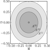
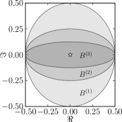
Figure 1: Numerical ranges $W(A^{(1)}),W(A^{(2)}),W(A^{(3)})$ from Example 2 for $p=0.5$ and $W(B^{(1)}),W(B^{(2)}),W(B^{(3)})$ from Example 3 for $p=0.25$. The stars mark the barycenter points in these examples. They are preserved by the dynamics.

Example 3. Let again $N=2$. The phase-flip channel is the discrete dynamics $\Psi=\Phi_{X_{1},X_{2}}$ corresponding to the Kraus operators $X_{1}=\sqrt{1-p}\;{\mathbf{1}}_{2}$ and $X_{2}=\sqrt{p}\sigma_{1}$. Here again, $p\in(0,1)$ is a free parameter. We set $B^{(1)}=A^{(1)}$ and $B^{(j+1)}=\Psi^{j}(B^{(1)})$. Then $B^{(2)}=\left[\begin{array}[]{cc}0&1-p\\ p&0\\ \end{array}\right]$ and $B^{(3)}=\left[\begin{array}[]{cc}0&1-2p(1-p)\\ 2p(1-p)&0\\ \end{array}\right]$. The numerical ranges of all $B^{(j)}$ are ellipses. Fig. 1b shows $W(B^{(1)}),W(B^{(2)}),W(B^{(3)})$ for $p=0.25$.

Example 4. This example is a generalization of Example 3 to $N=3$. The double flip channel acting on a qutrit is the the discrete dynamics $\Xi=\Phi_{X_{1},X_{2},X_{3}}$; the Kraus operators are $X_{1}=\sqrt{1-p-q}\mathbf{1}_{3}$, $X_{2}=\sqrt{p}\left[\begin{array}[]{ccc}0&1&0\\ 1&0&0\\ 0&0&1\\ \end{array}\right]$ and $X_{3}=\sqrt{q}\left[\begin{array}[]{ccc}1&0&0\\ 0&0&1\\ 0&1&0\\ \end{array}\right]$. The parameters $p,q$ satisfy $0\leq p,q,\,p+q\leq 1$. The operators $X_{2}$ and $X_{3}$ correspond to bit flips with probabilities $p$ and $q$. The operator $\Xi$ is trace preserving. The operator $C^{(1)}=\left[\begin{array}[]{ccc}0&1&0\\ 0&1&0\\ 0&0&2i\\ \end{array}\right]$ was studied in [16]; the numerical range $W(C^{(1)})$ is an ellipse. The barycenter of $W(C^{(1)})$ is $\rm{tr}(C^{(1)})/3=(1+2i)/3$. Set $C^{(j)}=\Xi^{j-1}(C^{(1)})$. For instance, $C^{(2)}=\left[\begin{array}[]{ccc}p&1-p-q&q\\ p&1-p-q(1-2i)&0\\ 0&0&2i+q(1-2i)\\ \end{array}\right]$. In Figure  2 $p=0.5$ and $q=0.4$, hence $1-p-q=0.1$.

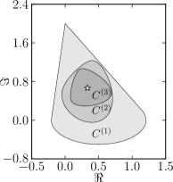
Figure 2: This figure illustrates Example 4 and the inclusion relation  (18). It shows the numerical ranges $W(C^{(1)}),W(C^{(2)}),W(C^{(3)})$ for $p=0.5$ and $q=0.4$. The limit of $W(C^{(j)})$, as $j\to\infty$, is the barycenter point $(1+2i)/3$ marked by the star.

4 Joint numerical shadows

We will first recall the notion of the numerical shadow of an operator on $\mathcal{H}_{N}$ [14, 13]. Let $\mu$ be the normalized Haar measure on $S(\mathcal{H}_{N})=\{\psi\in\mathcal{H}_{N}:||\psi||=1\}$, i.e., the unit sphere $S^{2N-1}$. We also denote by $\mu$ its push-forward to $\Omega_{N}\simeq\mathbb{C}P^{N-1}$. Let $A\in\mathcal{L}_{N}$. The numerical shadow $\nu_{A}$ is the push-forward of $\mu$ to $\mathbb{C}$ under the numerical range map. If $dz$ denotes the Lebesgue measure on $\mathbb{C}$, then $d\nu_{A}(z)=P_{A}(z)dz$ where

$$P_{A}(z)=\ \int_{\Omega_{N}}{\rm d}\mu(\psi)\ \delta\Bigl{(}z-\langle\psi|A|\psi\rangle\Bigr{)}$$ (22)

is a probability distribution.

Let now $A_{1},\dots,A_{m}\in\mathcal{M}_{N}$. Their joint numerical shadow $\nu_{A_{1},\dots,A_{m}}$ is the push-forward of $\mu$ under the joint numerical range map ${\rm jnr}_{(A_{1},\dots,A_{m})}:\Omega_{N}\to\mathbb{R}^{m}$. Thus, $\nu_{A_{1},\dots,A_{m}}$ is a probability measure supported on $W(A_{1},\dots,A_{m})$. Let $dx^{m}$ denote the Lebesgue measure on $\mathbb{R}^{m}$. Then $d\nu_{A_{1},\dots,A_{m}}=P_{A_{1},\dots,A_{m}}(x_{1},\dots,x_{m})dx^{m}$ where

$$P_{A_{1},\dots,A_{m}}(x_{1},\dots,x_{m})=\int_{\Omega_{N}}{\rm d}\mu(\psi)\ \prod_{j=1}^{m}\delta\Bigl{(}x_{j}-\langle\psi|A_{j}|\psi\rangle\Bigr{)}.$$ (23)

is a probability distribution. Numerical shadow is the special case of the joint numerical shadow corresponding to $m=2$. See the examples below for illustration.

Let $k_{1},\dots,k_{m}\in\mathbb{N}$. The moments

$$I_{k_{1},\dots,k_{m}}(A_{1},\dots,A_{m})=\int_{\mathbb{R}^{m}}x_{1}^{k_{1}}\cdots x_{m}^{k_{m}}d\nu_{A_{1},\dots,A_{m}}(x_{1},\dots,x_{m}).$$ (24)

are well defined and, by the Stone-Weierstrass theorem, uniquely determine the joint numerical shadow. When $m=2$, we recover the moments of the numerical shadow $\nu_{A}$ for the matrix $A=A_{1}+iA_{2}\in\mathcal{L}_{N}$ introduced in  [14]. Some of the results in  [14] extend to the moments of joint numerical shadows for arbitrary $m$. We will report on this in a separate publication.

If $\nu$ is a measure on $\mathbb{R}^{m}$ and $a\in\mathbb{R}$, we denote by $\nu^{a}$ the push-forward of $\nu$ under the self-map $v\mapsto av$ of $\mathbb{R}^{m}$. If $\nu_{1},\nu_{2}$ are measures on $\mathbb{R}^{m}$, we denote by $\nu_{1}*\nu_{2}$ their convolution. The following proposition exposes a few basic properties of joint numerical shadows. We leave the proof to the reader.

Proposition 3

1. Let $A_{1},\dots,A_{m}\in\mathcal{M}_{N}$. Let $U\in\mathcal{L}_{N}$ be a unitary operator. Set $B_{i}=UA_{i}U^{*},1\leq i\leq m$. Then

$$\nu_{B_{1},\dots,B_{m}}=\nu_{A_{1},\dots,A_{m}}.$$

2. Let $A_{1},\dots,A_{m}\in\mathcal{M}_{N}$ and $B_{1},\dots,B_{m}\in\mathcal{M}_{N}$ be arbitrary. Let $a,b\in\mathbb{R}$. Then

$$\nu_{aA_{1}+bB_{1},\dots,aA_{m}+bB_{m}}=\nu_{A_{1},\dots,A_{m}}^{a}*\nu_{B_{1},\dots,B_{m}}^{b}.$$

Example 5. We review Example 1. The set $W(\sigma_{1},\sigma_{2},\sigma_{3})\subset\mathbb{R}^{3}$ is the unit sphere. The joint numerical shadow $\nu_{\sigma_{1},\sigma_{2},\sigma_{3}}$ is the normalized Haar measure.

Example 6. We use the isomorphism $\mathcal{H}_{4}=\mathcal{H}_{2}\otimes\mathcal{H}_{2}$ to define the extensions of Pauli matrices $A_{j}=\sigma_{j}\otimes{\mathbf{1}}_{2},\,j=1,2,3$. We use the fact that the Haar measure on the space of pure states in ${\mathcal{H}}_{A}\otimes{\mathcal{H}}_{B}$ induces by partial trace, $\omega={\rm Tr}_{B}|\psi\rangle\langle\psi|$, the Lebesgue measure on the space of mixed states in $\mathcal{H}_{2}$ [20]. Using the equality between the expected values of an operator on $\mathcal{H}_{2}$ and the extended operator on $\mathcal{H}_{4}$, we obtain that $\nu_{A_{1},A_{2},A_{3}}$ is the normalized Lebesgue measure on the Bloch ball. Let $B_{j}={\mathbf{1}}_{2}\otimes\sigma_{j},\,j=1,2,3$. The swap operator

$$S=\left[\begin{array}[]{cccc}1&0&0&0\\ 0&0&1&0\\ 0&1&0&0\\ 0&0&0&1\\ \end{array}\right],$$ (25)

is a unitary operator on $\mathcal{H}_{4}$ satisfying $B_{j}=SA_{j}S^{*}$. By Proposition  3 and the above discussion, $\nu_{B_{1},B_{2},B_{3}}$ is the normalized Lebesgue measure on the Bloch ball.

Acknowledgements. This project started at the 43th Symposium on Mathematical Physics in Toruń; it was accomplished during the 44th Symposium. It is a pleasure to thank the organizers of these Symposia. We are obliged to Piotr Gawron for creating the figures. K. Ż. is grateful to C. F. Dunkl, J. A. Holbrook, J. Miszczak and Z. Puchała for fruitful discussions on numerical shadows and acknowledges financial support by the grant N202 090239 of the Polish Ministry of Science and Higher Education. The work of E.G. was partially supported by the MNiSzW grant N N201 384834 and the NCN Grant DEC-2011/03/B/ST1/00407. He acknowledges stimulating discussions with Bent Orsted in Aarhus in June 2011. Finally, we thank the anonymous referee for comments and suggestions.

References

[1]
A. Horn and C. R. Johnson,
Topics in Matrix Analysis,
Cambridge University Press, Cambridge, 1994.
[2]
K. E. Gustafson and D. K. M. Rao.
Numerical Range: The Field of Values of Linear Operators and
Matrices.
Springer-Verlag, New York, 1997.
[3] O. Toeplitz, Das algebraische Analogon zu einem
Satze von Fejér, Math. Zeitschrift 2 (1918), 187–197.
[4] F. Hausdorff, Der Wertvorrat einer
Bilinearform, Math. Zeitschrift 3 (1919), 314–316.
[5] E. Gutkin,
The Toeplitz-Hausdorff theorem revisited: relating linear algebra and geometry,
Math. Intelligencer26, 8 – 14 (2004).
[6] E. Jonckheere, F. Ahmad, E. Gutkin,
Differential topology of numerical range,
Lin. Alg. Appl.279, 227 – 254 (1998).
[7] C. K. Li,
A simple proof of the elliptical range theorem,
Proc. Am. Math. Soc.124, 1985-1986 (1996).
[8] D.S. Keeler, L. Rodman and I.M. Spitkovsky,
The numerical range of matrices,
Lin. Alg. Appl.252, 115-1139 (1997).
[9] D. W. Kribs, A. Pasieka, M. Laforest, C. Ryan, and M. P. Silva,
Research problems on numerical ranges in quantum computing,
Linear and Multilinear Algebra57, 491-502 (2009).
[10]
T. Schulte-Herbrüggen, G. Dirr, U. Helmke, and S. J. Glaser,
The significance of the -numerical range and the local
c-numerical range in quantum control and quantum information,
Linear and Multilinear Algebra56, 3-26 (2008)
[11] P. Gawron, Z. Puchała, J. A. Miszczak,
Ł. Skowronek, M.-D. Choi, and K. Życzkowski,
Restricted numerical range: a versatile tool in the theory of quantum information,
J. Math. Phys.51, 102204 (24pp) (2010).
[12] C.F. Dunkl, P. Gawron, J.A. Holbrook, J. Miszczak,
Z. Puchała and K. Życzkowski,
Numerical shadow and geometry of quantum states,
J. Phys.A 44, 335301 (19pp) (2011).
[13] T. Gallay and D. Serre,
Numerical measure of a complex matrix,
Commun. Pure Apl. Math.65, 287-336 (2012).
[14] C.F. Dunkl, P. Gawron, J.A. Holbrook, Z. Puchała and K. Życzkowski,
Numerical shadows: Measures and densities on the numerical range,
Lin. Algebra Appl434, 2042-2080 (2011).
[15] K. Życzkowski (with M.–D. Choi, C. Dunkl, J. Holbrook, P. Gawron,
J.Miszczak, Z. Puchała, and L. Skowronek),
Generalized numerical range as a versatile tool to study quantum entanglement,
Oberwolfach Report59, 34–37 (2009).
[16] Z. Puchała, J. A. Miszczak, P. Gawron,
C. F. Dunkl, J. A. Holbrook, and K. Życzkowski,
Restricted numerical shadow and geometry of quantum entanglement,
J. Phys.A 45, 415309 (28pp) (2012).
[17] E. Gutkin, E.A. Jonckheere, M. Karrow,
Convexity of the joint numerical range:
topological and differencial geometric viewpoints,
Lin. Alg. Appl.376, 143 – 171 (2004).
[18] I. Bengtsson and K. Życzkowski,
Geometry of Quantum States, Cambridge UP, Cambridge, 2006.
[19] L. I. Schiff, Quantum Mechanics,
New York, McGraw-Hill 1968.
[20] K. Życzkowski and H.-J. Sommers,
Induced measures in the space of mixed quantum states,
J. Phys.A 34, 7111-7125 (2001).