Abstract

We revisit the quantized version of the harmonic oscillator obtained through a $q$-dependent family of coherent states. For each $q$, $0<q<1$, these normalized states form an overcomplete set that resolves the unity with respect to an explicit measure. We restrict our study to the case in which $q^{-1}$ is a quadratic unit Pisot number: the $q$-deformed integers form Fibonacci-like sequences of integers. We then examine the main characteristics of the corresponding quantum oscillator: localization in the configuration and in the phase spaces, angle operator, probability distributions and related statistical features, time evolution and semi-classical phase space trajectories.

PACS: 03.65.Fd; 03.65.Sq; 02.30.Cj

Keywords: Coherent states; $q$-calculus; moment problem; quantization; quadratic Pisot number.

1 Introduction

In this work we revisit non-linear coherent states obtained from the standard ones through a certain type of $q$– or $q\,p$–deformations of the integers. Similar deformations have already been considered during the two last decades, since the pioneering work by Arik et al [1] (see for instance [2, 3, 4, 5] and references therein for a list of more recent related works, mostly devoted to algebraic aspects of such deformations). Our aim is to use these deformed coherent states for quantizing à la Berezin-Klauder-Toeplitz elementary classical observables like position, momentum, angle, quadratic Hamiltonian etc, and to examine some interesting features of their quantum counterparts. In particular, we insist on the condition that our (symmetric) $q$-deformations of integers be still integers, more precisely yield sequences of integers that generalize the famous Fibonacci sequence.

Section 2 is a review of what we understand by quantization of a centered disk of finite radius or of the complex plane $\mathbb{C}$, both being viewed as possible phase spaces for one degree of freedom mechanical systems. We then study in Section 3 sequences of integer numbers that appear as $q\,p$-deformations of integer numbers. We present two types of such sequences that we call fermionic (or antisymmetric) and bosonic (or symmetric) sequences. In both cases $p$ and $q$ are quadratic Pisot (more fairly Pisot-Vijayaraghavan) numbers. Among these appears the well-known Fibonacci sequence. We specially concentrate our study upon sequences of integers $({}^{s}[n]_{q})_{n\in\mathbb{N}}$ encountered in symmetric $q$-deformations of integers. Section 4 is devoted to the resolution of the moment problem (2.2), i.e, to finding a positive measure $w_{q}(t)\,dt$ such that ${}^{s}[n]_{q}!=\int_{0}^{\infty}t^{n}\,w_{q}(t)\,dt$. In Section 5 we present some computations and graphics for different $q$-sequences showing the main physical properties of these $q$-CS and the exceptional Pisot cases leading to nice periodic phase trajectories for lower symbols of time-evolving position and momentum operators issued from CS quantization. In the conclusion we give some remarks and put our work into the perspective of the general coherent state quantization framework. Finally four appendices are devoted to an introduction to the standard $q$-calculus, the symmetric $q$-calculus, the equations determining the quadratic Pisot numbers and powers and recurrence for general quadratic Pisot numbers.

2 A review of non-linear CS quantization issued from sequences of numbers

Let us suppose that we observe through some experimental device an infinite, strictly increasing sequence of nonnegative real numbers $\left(x_{n}\right)_{n\in\mathbb{N}}$, such that $x_{0}=0$, for instance the quantum energy spectrum of a given system, but it could be some other kind of observed data. To this sequence of numbers there corresponds the sequence of “factorials” $x_{n}!:=x_{1}\times x_{2}\times\dotso\times x_{n}$ with $x_{0}!:=1$. An associated exponential can be defined by

$$\mathcal{N}(t):=\sum_{n=0}^{+\infty}\frac{t^{n}}{x_{n}!}\,.$$ (2.1)

We assume that it has a nonzero convergence radius $R=\lim_{n\to\infty}x_{n+1}$. We now suppose that the (Stieltjes) moment problem has a (possibly non unique) solution for the sequence of factorials $\left(x_{n}!\right)_{n\in\mathbb{N}}$, i.e. there exists a probability distribution $t\mapsto w(t)$ on $[0,R)$ such that

$$x_{n}!=\int_{0}^{R}t^{n}\,w(t)\,dt\,,$$ (2.2)

and we extend (formally) the definition of the function $n\mapsto x_{n}!$ to real or complex numbers when it is needed (and possible!). Let $\mathcal{H}$ be a separable (complex) Hilbert space with scalar product $\langle\cdot|\cdot\rangle$ and orthonormal basis $|e_{0}\rangle,|e_{1}\rangle,\dotsc,|e_{n}\rangle,\dotsc$, i.e.,

$$\langle e_{n}|e_{n^{\prime}}\rangle=\delta_{nn^{\prime}}\,,\qquad\sum_{n\geq 0}|e_{n}\rangle\langle e_{n}|=I_{d}.$$ (2.3)

To each complex number $z$ in the open disk $\mathcal{D}_{\sqrt{R}}=\{z\in\mathbb{C}\,,\,|z|<\sqrt{R}\}$ we associate a vector in $\mathcal{H}$ defined as:

$$|v_{z}\rangle=\sum_{n=0}^{\infty}\frac{1}{\sqrt{\mathcal{N}(|z|^{2})}}\frac{z^{n}}{\sqrt{x_{n}!}}\,|e_{n}\rangle\,.$$ (2.4)

These vectors enjoy the following properties similar to those obeyed by standard coherent states (CS) [6, 7]:

• $\|v_{z}\|=1$ (normalization).

• The map $\mathcal{D}_{\sqrt{R}}\ni z\mapsto|v_{z}\rangle$ is weakly continuous (continuity).

• The map $\mathbb{N}\in n\mapsto|\langle e_{n}|v_{z}\rangle|^{2}=\dfrac{|z|^{2n}}{\mathcal{N}(|z|^{2})\;x_{n}!}$ is a Poisson-like distribution in $|z|^{2}$, with average number of events equal to $|z|^{2}$ (discrete probabilistic content).

• The map $\mathcal{D}_{\sqrt{R}}\ni z\mapsto|\langle e_{n}|v_{z}\rangle|^{2}=\dfrac{|z|^{2n}}{\mathcal{N}(|z|^{2})\;x_{n}!}$ is a (gamma-like) probability distribution (with respect to the square of the radial variable) with $x_{n+1}$ as a shape parameter and with respect to the following measure on the open disk $\mathcal{D}_{\sqrt{R}}$ (continuous probabilistic content [8])

  $$\nu(d^{2}z):=\mathcal{N}(|z|^{2})\,w(|z|^{2})\frac{d^{2}z}{\pi}\,,$$ (2.5)

  where $d^{2}z=d\,{\rm Re}z\;d\,{\rm Im}z$.

• The family of vectors (2.4) resolves the unity :

  $$\int_{\mathcal{D}_{\sqrt{R}}}\nu(d^{2}z)\,|v_{z}\rangle\langle v_{z}| =\sum_{n,n^{\prime}=0}^{\infty}|e_{n}\rangle\langle e_{n^{\prime}}|\,\frac{1}{\sqrt{x_{n}!x_{n}^{\prime}!}}\,\int_{\mathcal{D}_{\sqrt{R}}}\dfrac{d^{2}z}{\pi}\,w(|z|^{2})z^{n}{\bar{z}}^{n^{\prime}}$$

  $$=\sum_{n=0}^{\infty}|e_{n}\rangle\langle e_{n}|\,\frac{1}{x_{n}!}\,\int_{0}^{R}dt\,w(t)\;t^{n}=I_{d}\,,$$ (2.6)

  with the last equality resulting trivially from (2.2) and (2.3).

Vectors (2.4) are known in the literature as “non-linear” coherent states, an attributive adjective essentially issued from Quantum Optics [9, 10, 11, 12] (see also [13] for exhaustive references).

Property (v) is fundamental for quantization of the open disk $\mathcal{D}_{\sqrt{R}}$ in the sense that it allows one to define:

1. a normalized positive operator-valued measure (POVM) on $\mathcal{D}_{\sqrt{R}}$ equipped with the measure $\nu(d^{2}z)$ (2.5) and its $\sigma-$algebra $\mathcal{F}$ of Borel sets :

   $$\mathcal{F}\ni\Delta\,\mapsto\int_{\Delta}\nu(d^{2}z)\,|v_{z}\rangle\langle v_{z}|\,\,\in\mathcal{L}(\mathcal{H})^{+}\,,$$

   where $\mathcal{L}(\mathcal{H})^{+}$ is the cone of positive bounded operators on $\mathcal{H}$;

2. a Berezin-Klauder-Toeplitz (or “anti-Wick”) quantization, simply named coherent state quantization throughout this paper, of the complex plane [14, 15, 16, 7], which means that to a function $f(z,\bar{z})$ in the complex plane corresponds the operator $A_{f}$ in $\mathcal{H}$ defined by

   $$f\mapsto A_{f}=\int_{\mathcal{D}_{\sqrt{R}}}\nu(d^{2}z)\,f(z,\bar{z})\,|v_{z}\rangle\langle v_{z}|=\sum_{n,n^{\prime}=0}^{\infty}\left(A_{f}\right)_{nn^{\prime}}\,|e_{n}\rangle\langle e_{n^{\prime}}|\,,$$ (2.7)

   with matrix elements

   $$\left(A_{f}\right)_{nn^{\prime}}=\frac{1}{\sqrt{x_{n}!x_{n^{\prime}}!}}\,\int_{\mathcal{D}_{\sqrt{R}}}\frac{d^{2}z}{\pi}\,w(|z|^{2})\,f(z,\bar{z})\,z^{n}{\bar{z}}^{n^{\prime}}\,.$$

   The operator-valued integral (2.7) is understood as the sesquilinear form,

   $$B_{f}(\psi_{1},\psi_{2})=\int_{\mathcal{D}_{\sqrt{R}}}\nu(d^{2}z)\,f(z,\bar{z})\,\langle\psi_{1}|v_{z}\rangle\langle v_{z}|\psi_{2}\rangle.$$

   The form $B_{f}$ is assumed to be defined on a dense subspace of the Hilbert space. If $f$ is real and at least semi-bounded, the Friedrich’s extension of $B_{f}$ univocally defines a self-adjoint operator. However, if $f$ is not semi-bounded, there is no natural choice of a self-adjoint operator associated with $B_{f}$. In this case, we can consider directly the symmetric operator $A_{f}$ enabling us to obtain a self-adjoint extension (unique for particular operators). The question of what is the class of operators that may be so represented is a subtle one. We will come back to this point in Definition 2.1 below.

   If the function $f$ depends on $|z|^{2}=t$ only, we get (formally) a diagonal operator with matrix elements

   $$\left(A_{f}\right)_{nn^{\prime}}=\frac{\delta_{nn^{\prime}}}{x_{n}!}\,\int_{0}^{R}dt\,w(t)\,t^{n}\,f(t)\,.$$

   On the other hand, if $f$ depends on the angle $\theta=\arg z$ only, i.e. $f(z,\bar{z})=F(\theta)$, the matrix elements of $A_{f}$ involve the Fourier coefficients

   $$c_{n}(F)=\displaystyle\frac{1}{2\pi}\int_{0}^{2\pi}d\theta\,e^{-in\theta}\,F(\theta),$$

   i.e.

   $$\left(A_{F}\right)_{nn^{\prime}}=c_{n^{\prime}-n}(F)\,\frac{x_{\frac{n+n^{\prime}}{2}}!}{\sqrt{x_{n}!\;x_{n^{\prime}}!}}\,.$$

   For instance, the following self-adjoint “angle” operator is defined in this way. Its matrix elements are given by:

   $$A_{\theta}=\pi\,I_{{\mathcal{H}}}+i\,\sum_{n\neq n^{\prime}}\frac{x_{\frac{n+n^{\prime}}{2}}!}{\sqrt{x_{n}!\;x_{n^{\prime}}!}}\,\frac{1}{n^{\prime}-n}\,|e_{n}\rangle\langle e_{n^{\prime}}|\,,$$ (2.8)

   where we recall that $x_{\nu}!$ is defined by $x_{\nu}!=\int_{0}^{R}dt\,w(t)\,t^{\nu}$ whenever the latter integral converges.

For the elementary functions $f(z,\bar{z})=z$ and $f(z,\bar{z})=\bar{z}$ we obtain lowering and raising operators, respectively,

$$A_{z} =a\,,\;\qquad a\,|e_{n}\rangle=\sqrt{x_{n}}|e_{n-1}\rangle\,,\quad\;a\,|e_{0}\rangle=0\,\quad\mbox{(lowering operator)},$$ (2.9)

$$A_{\bar{z}} =a^{{\dagger}}\,,\qquad a^{{\dagger}}\,|e_{n}\rangle=\sqrt{x_{n+1}}|e_{n+1}\rangle\qquad\qquad\qquad\mbox{(raising operator)}\,.$$ (2.10)

It results that the state $|v_{z}\rangle$ is eigenvector of $A_{z}=a$ with eigenvalue $z$ (i.e. $a|v_{z}\rangle=z|v_{z}\rangle$) like for standard CS. Operators $a$ and $a^{{\dagger}}$ obey the generically non-canonical commutation rule

$$[a,a^{{\dagger}}]=x_{N+1}-x_{N},$$

where the “deformed-number” operator $x_{N}$ is defined by $x_{N}=a^{{\dagger}}a$ and is such that its spectrum is exactly $\{x_{n}\,,\,n\in\mathbb{N}\}$ with eigenvectors $x_{N}\,|e_{n}\rangle=x_{n}|e_{n}\rangle$. The linear span of the triple $\{a,a^{{\dagger}},x_{N}\}$ is obviously not closed, in general, under commutation and the set of resulting commutators generically gives rise to an infinite dimensional Lie algebra. These algebraic structures were extensively examined in previous papers (e.g. [1]).

The next simplest function on the complex plane is $f(z,\bar{z})=|z|^{2}$. When we consider the complex plane as the phase space of a particle moving on the line, i.e. $z=\frac{1}{\sqrt{2}}(\mathbf{q}+i\mathbf{p})$ and, hence, $|z|^{2}=\frac{1}{2}(\mathbf{p}^{2}+\mathbf{q}^{2})$ we get, in appropriate units, the classical Hamiltonian of the harmonic oscillator (H.O.). In this case

$$A_{z\bar{z}}=A_{z}\,A_{\bar{z}}=a\,a^{{\dagger}}=x_{N+1}\,.$$

Therefore, the spectrum of the quantized version of $|z|^{2}$ is the sequence $\left(x_{n}\right)_{n\geq 1}$.

Let us consider the (deformed) position and momentum operators as the respective CS quantizations of the phase space coordinates $\mathbf{q}$ and $\mathbf{p}$:

$$A_{\mathbf{q}}\equiv Q=\frac{1}{\sqrt{2}}(a+a^{\dagger})\;,\qquad A_{\mathbf{p}}\equiv P=\frac{1}{i\sqrt{2}}(a-a^{\dagger})\;.$$ (2.11)

It is worthy to note that if we had adopted the usual procedure of the canonical quantization for defining the quantum version of a classical observable $f(\mathbf{q},\mathbf{p})$, namely replacing $\mathbf{q}$ and $\mathbf{p}$ by $Q$ and $P$ respectively in the latter and proceeding with the symmetrization of $f(Q,P)$, we would have obtained expressions in general different of $A_{f}$. In the case of simple quadratic expressions these discrepancies read as

$$A_{q^{2}}=Q^{2}+\frac{1}{2}(x_{N+1}-x_{N})\,,\quad A_{p^{2}}=P^{2}+\frac{1}{2}(x_{N+1}-x_{N})\,,$$ (2.12)

and so for the H.O. Hamiltonian,

$$\frac{1}{2}(P^{2}+Q^{2})=A_{(p^{2}+q^{2})/2}-\frac{1}{2}(x_{N+1}-x_{N})=\frac{1}{2}(x_{N+1}+x_{N})\,.$$ (2.13)

Now an energy is always defined up to a constant. One usually decides that the zero-point of quantum energies lies at the infimum of the spectrum ($\sigma$) of the quantum potential energy. In the case of the canonical quantization, the latter is $\inf\sigma(Q^{2}/2)$ whilst it is $\inf\sigma((Q^{2}+x_{N+1}-x_{N})/2)$ in the case of CS quantization. So we have to compare the spectral values $x_{n}-\inf\sigma(Q^{2}/2)$ (for the canonical quant.) with $x_{n+1}-\inf\sigma((Q^{2}+x_{N+1}-x_{N})/2)$ (for the CS quant.). To solve this problem, we need to know more about the sequence $(x_{n})$. In the non-negative integer case, the two above differences are identical.

Given a function $f$ on the complex plane, the resulting operator $A_{f}$, if it exists, at least in a weak sense, acts on the Hilbert space ${\mathcal{H}}$. The integral

$$\langle\psi|A_{f}|\psi\rangle=\int_{\mathcal{D}_{\sqrt{R}}}f(z,\bar{z})|\langle\psi|v_{z}\rangle|^{2}\,\nu(d^{2}z)$$

should be finite for all $\psi$ in some dense subset of $\mathcal{H}$. In order to be more rigorous on this important point, let us adopt the following acceptance criteria for a function to belong to the class of quantizable classical observables.

Definition 2.1

A function $\mathcal{D}_{\sqrt{R}}\ni z\mapsto f(z,\bar{z})\in\mathbb{C}$ is a CS quantizable classical observable via the map $f\mapsto A_{f}$ defined by (2.7) if the map $\mathcal{D}_{\sqrt{R}}\ni z=\frac{1}{2}(\mathbf{q}+i\mathbf{p})\equiv(\mathbf{q},\mathbf{p})\mapsto\langle v_{z}|A_{f}|v_{z}\rangle$ is a smooth (i.e. $C^{\infty}$) function with respect to the $(\mathbf{q},\mathbf{p})$ coordinates.

The function $f$ is the upper [18] or contravariant [15] symbol of the operator $A_{f}$, and the mean value of the latter in state $|v_{z}\rangle$,

$$\check{f}(z,\bar{z}):=\langle v_{z}|A_{f}|v_{z}\rangle=\int_{\mathcal{D}_{\sqrt{R}}}f(z^{\prime},\bar{z^{\prime}})|\langle v_{z}|v_{z^{\prime}}\rangle|^{2}\,\nu(d^{2}z^{\prime})\,,$$

is the lower [18] or covariant [15] symbol of the operator $A_{f}$. The map $f\mapsto\check{f}$ is an integral transform with kernel $|\langle v_{z}|v_{z^{\prime}}\rangle|^{2}$ which generalizes the Berezin transform.

In [17] the definition 2.1 in the standard case $x_{n}=n$ is extended to a class of distributions including tempered distributions.

Localization properties in the complex plane, from the point of view of the sequence $\{x_{n}\}_{n\in\mathbb{N}}$, should be examined through the shape (as functions of $z$) of the respective lower symbols of $Q$ and $P$:

$$\check{Q}(z):=\langle v_{z}|Q|v_{z}\rangle\,,\qquad\check{P}(z):=\langle v_{z}|P|v_{z}\rangle\,,$$

and the noncommutativity reading of the complex plane should be encoded in the behaviour of the lower symbol $\langle v_{z}|[Q,P]|v_{z}\rangle$ of the commutator $[Q,P]$. The dispersions verify

$$\left(\Delta_{v_{z}}Q\right)^{2}=\left(\Delta_{v_{z}}P\right)^{2}=\frac{1}{2}\,\langle v_{z}|(x_{N+1}-x_{N})|v_{z}\rangle=\frac{1}{2}|\langle v_{z}|[Q,P]|v_{z}\rangle|$$ (2.14)

for any $|v_{z}\rangle$, which indicates that the latter form a family of intelligent states. The study, within the above framework, of the product of dispersions expressed in states $|v_{z}\rangle$,

$$\left(\Delta_{v_{z}}Q\right)\,\left(\Delta_{v_{z}}P\right)=\frac{1}{2}\,\langle v_{z}|(x_{N+1}-x_{N})|v_{z}\rangle\,,$$ (2.15)

should thus be relevant since they saturate the uncertainty relations within the quantization context provided by them. Note that eq. (2.15) can also be written in terms of mean values $\langle F(n)\rangle$ of discrete function $n\mapsto F(n)$ with respect to the Poisson-like distribution $n\mapsto\dfrac{t^{n}}{\mathcal{N}(t)\;x_{n}!}$:

$$\left(\Delta_{v_{z}}Q\right)\,\left(\Delta_{v_{z}}P\right)=\frac{1}{2}\,\langle(x_{n+1}-x_{n})\rangle=\frac{1}{2}\,\left(\langle x_{n+1}\rangle-|z|^{2}\right)\,.$$

Another interesting function emerging from this formalism is the lower symbol of a function $F(\theta)$ of the angle only. With $z=re^{i\theta}$ we find the series

$$\check{F}(z,\bar{z})=\langle v_{z}|A_{F}|v_{z}\rangle=c_{0}(F)+\sum_{k\neq 0}d_{|k|}(r)\,c_{k}(F)\,e^{ik\theta}\,,$$ (2.16)

where the function

$$d_{|k|}(r)=\frac{r^{k}}{\mathcal{N}(r^{2})}\sum_{n=0}^{\infty}\frac{x_{\frac{|k|}{2}+n}!}{x_{n}!\;x_{n+|k|}!}\,r^{2n}$$ (2.17)

balances the Fourier coefficient $c_{k}(F)$ of the function $F$ (see Appendix A).

Thus for the angle operator $A_{\theta}$ (2.8) we have the particular series (see Fig. 12a):

$$\check{\theta}(z,\bar{z})=\pi+i\sum_{k\in\mathbb{Z}-\{0\}}\frac{d_{|k|}(r)}{k}\,e^{ik\theta}\,=\pi-2\sum_{k=1}^{\infty}\frac{d_{|k|}(r)}{k}\,\sin({k\theta})\,.$$ (2.18)

Note that if we wish to restore physical units, e.g. for the motion of a particle (mass $m$) on the line, we should introduce some characteristic length and momentum which will provide unit standard for the $(\mathbf{q},\mathbf{p})$ variables, say $\ell_{c}$ and $\wp_{c}$ respectively. Since we have in view a (CS) quantum version of this motion, it is natural to impose the relation $\ell_{c}\,\wp_{c}=\hbar$. So we keep dimensionless the phase space variable $z$ by putting

$$z=\frac{1}{\sqrt{2}}\left(\frac{\mathbf{q}}{\ell_{c}}+i\ell_{c}\frac{\mathbf{p}}{\hbar}\right)\,.$$ (2.19)

It is clear from the above expression that the (semi-)classical regime corresponds to large $|z|=r$ and that the original function $F(\theta)$ is recovered through its Fourier series if $\lim_{r\to\infty}d_{k}(r)=1$ for each $k$.

Let us tell more about the physical meaning of such a coherent state quantization, although if we go back to dimensionless quantities for the sake of simplicity. In the case of the sequence of non-negative integers, we have $x_{n}=n$, $R=\infty$ and we recover the canonical quantization of the complex plane $\mathcal{D}_{\infty}=\mathbb{C}$ viewed as the classical phase space for the motion of a particle on the line, equipped with the usual Lebesgue (or “uniform”) measure $\nu(d^{2}z)=d^{2}z/\pi$. Within this standard scheme, the quantized version of the classical H.O. Hamiltonian $H=\frac{1}{2}(\mathbf{p}^{2}+\mathbf{q}^{2})$ is the number operator $N+1$ with spectrum $1,2,\dotsc$. Also, one can prove in this case that $\lim_{r\to\infty}d_{k}(r)=1$ for each $k$ (see Fig. LABEL:fig_drka). Now, changing the measure $d^{2}z/\pi$ into

$$\nu(d^{2}z)=w(|z|^{2})\,\mathcal{N}(|z|^{2})\,\mathrm{H}(|z|^{2}-R)\,d^{2}z/\pi,$$

where $\mathrm{H}(\cdot)$ is the Heaviside function, we give to the phase space a different statistical content: classical states are not anymore described by points $z_{0}$, i.e. by Dirac distributions $z\mapsto\delta_{z_{0}}(z)$, but instead by the distribution $z\mapsto w(|z-z_{0}|^{2})\mathcal{N}(|z-z_{0}|^{2})\,\mathrm{H}(|z|^{2}-R)$. Then, by following the CS quantization stemming from the associated sequence $\left(x_{n}\right)_{n\in\mathbb{N}}$, we consistently find the latter as another (possibly observed!) energy spectrum along the equation

$$A_{\frac{1}{2}(p^{2}+q^{2})}=A_{z\bar{z}}=a\,a^{{\dagger}}=x_{N+1}\,.$$

Since we are dealing with a different quantized version of the classical observable $|z|^{2}$ and considering it as a quantum Hamiltonian $\hat{H}$, ruling the time evolution of quantum states, it is natural to investigate the time evolution of the quantized version $a=A_{z}$, as found in (2.9), of the classical phase space point $z=(\mathbf{q}+i\mathbf{p})/\sqrt{2}$, comparing it with the phase space circular classical trajectories. This time evolution is well caught through its mean value in coherent states $|v_{z}\rangle$ (lower symbol) :

$$\begin{array}[]{lll}\check{z}\left(t\right)&\overset{\mathrm{def}}{=}&\left\langle v_{z}\right|e^{-i\hat{H}t}\,A_{z}\,e^{i\hat{H}t}\left|v_{z}\right\rangle\\[8.5359pt] &=&\displaystyle\frac{z}{\mathcal{N}_{\lambda}(|z|^{2})}\sum_{n=0}^{+\infty}\frac{\left|z\right|^{2n}}{x_{n}!}\,\exp\left({i}\left({x_{n+2}-x_{n+1}}\right){t}\right)\,.\end{array}$$ (2.20)

In the standard case we just have $\check{z}\left(t\right)=e^{it}z$, which describes nothing else but the classical phase-space trajectory. In the deformed case (2.20) we easily prove that $|\check{z}\left(t\right)|\leq|z|$.

There exists another interesting exploration of the semi-classical character of coherent states. For this purpose we can define a phase space distribution in terms of the following density of probability (given a fixed a normalized state, say $|v_{z_{0}}\rangle$) on the complex plane equipped with the measure $d\nu(=d^{2}z)$ for all $t$ :

$$z=(q,p)/\sqrt{2}\in\mathbb{C}\mapsto\rho_{v_{z_{0}}}(z):=|\langle v_{z}|v_{z_{0}}\rangle|^{2}=\frac{|\mathcal{N}(\bar{z}z_{0})|^{2}}{\mathcal{N}(|z|^{2})\mathcal{N}(|z_{0}|^{2})}\,.$$ (2.21)

The time evolution behavior of the probability density $\rho_{v_{z_{0}}}(z)$ is given by

$$z\mapsto\rho_{v_{z_{0}}}(z,t):=|\langle v_{z}|e^{-i\hat{H}t}|v_{z_{0}}\rangle|^{2}=\frac{|\mathcal{N}_{\Delta_{N}\,t}(\bar{z}z_{0})|^{2}}{\mathcal{N}(|z|^{2})\mathcal{N}(|z_{0}|^{2})}\,,$$ (2.22)

where the modified “exponential” appearing at the numerator is defined by:

$$\mathcal{N}_{\Delta_{N}\,t}(z):=\sum_{n=0}^{\infty}\frac{z^{n}}{x_{n}!\;e^{i\Delta_{n}t}}\,,\quad\Delta_{n}=x_{n+1}\,.$$

3 Integers as deformations of integers

It is well-known that in the $q$-deformation of Lie algebras and in the study of their $q$-representations appear some real numbers that are deformations of nonnegative integer numbers like

$$[n]_{q}:=\frac{1-q^{\pm n}}{1-q^{\pm 1}},\qquad{}^{s}[n]_{q}:=\frac{q^{n}-q^{-n}}{q-q^{-1}},\quad n\in\mathbb{N},\;q\in\mathbb{R},$$ (3.23)

since in the limit $q\to 1$ we recover the original number $n$. For the $q$-oscillator these $q$-integer numbers constituted the energy spectrum of deformed versions of the harmonic oscillator ($0<|q|<1$). Moreover, $q$-coherent states are constructed for these $q$-oscillators.

In general, these sequences of $q$-numbers are non-integer numbers. Hence, one is naturally led to address the question: do there exist such sequences with $[n]_{q}\in\mathbb{N}\;\;\forall n\;\in\mathbb{N}$? For the previous $q$-deformation $[n]_{q}$ the answer is trivially no since if

$$[n]_{q}\equiv\frac{1-q^{n}}{1-q}=1+q+q^{2}+\cdots+q^{n-1}\quad\mbox{for any}\,n$$

then $q\in\mathbb{N}$.

However, there are other deformations of numbers where it is possible to obtain sequences of non-negative integers. The interest of such sequences would be to get, for instance, $qp$-harmonic oscillator with spectrum of positive integer numbers. As a matter of fact, let us consider the so-called $pq$-deformations of non-negative integers (or natural numbers) $n\in\mathbb{N}$:

$$[[n]]_{qp}:=\frac{q^{n}-p^{n}}{q-p}\,.$$

The particular cases $p=1$ and $p=q^{-1}$ correspond to $q$-deformations (3.23).

Now, we demand that the following property holds for any $n\in\mathbb{N}$:

$$u_{n}\equiv[[n]]_{qp}\in\mathbb{N}\,.$$

We already check that it is true for $u_{0}=0$ and $u_{1}=1$. From $q+p=u_{2}\in\mathbb{N}$ and $q^{2}+qp+p^{2}=u_{3}\in N$, we immediately infer that $q$ and $p$ are quadratic integers, i.e. both are roots of the quadratic equation

$$X^{2}-sX+r=0\,,\quad s=u_{2}=p+q\in\mathbb{N}\,,\quad r=pq=u_{2}^{2}-u_{3}\in\mathbb{N}\,.$$ (3.24)

We now impose that both $q$ and $p$ be non-zero real numbers. This implies that $0\leq s^{2}-4r=4u_{3}-3u_{2}^{2}=u_{3}-3r$. So, from $u_{3}\in\mathbb{N}$ and $r\in\mathbb{Z}$ we infer that $q$ and $p$ are real if $r<0$, i.e. $r$ is a negative integer. If $r>0$, i.e. $r$ is a positive integer, then $u_{3}$ should be bigger than $3r$. Hence, the choice of $r,s\in\mathbb{Z}^{\ast}$ determines completely the sequence of the $u_{n}$’s through a three-term recurrence which replicates exactly the algebraic equation (3.24). Indeed, by definition we have $u_{0}=0$, $u_{1}=1$ and $u_{2}=p+q$. Next,

$$u_{3}=(p+q)^{2}-qp=u^{2}_{2}-r=su_{2}-r,$$

and more generally, from the trivial identity,

$$p^{n+1}-q^{n+1}=(p+q)(p^{n}-q^{n})+pq(p^{n-1}-q^{n-1})\,$$

we have

$$u_{n+1}-su_{n}+ru_{n-1}=0\,,\quad u_{0}=0\,,\quad u_{1}=1\,.$$ (3.25)

Such sequences of numbers generalize the famous Fibonacci sequence corresponding to the simplest case $s=1$ and $r=-1$. In this case, $p=\dfrac{1+\sqrt{5}}{2}\equiv\tau$ (the golden mean) and $q=\dfrac{1-\sqrt{5}}{2}=-1/\tau$.

In this paper, we precisely focus on the cases $r=\pm 1$ and $s>0$ (the choice $s<0$ corresponding to a change of sign for both roots).

• Case 1.- If we choose $r=-1$, then $s\geq 1$, and the roots of

  $$X^{2}-sX-1=0\,$$

  are $q,p$ such that, say $-1<q<0$ and $1<p$.

• Case 2.- If we choose instead $r=1$, then $s\geq 2$ and the equation now reads

  $$X^{2}-sX+1=0\,.$$ (3.26)

  We exclude the trivial case $s=2$ which corresponds to $p=q=1$, and we will consider all other cases, $s\geq 3$, which give $0<q<1$ and $p=1/q>1$.

In both cases, the algebraic integer $p>1$ is called a quadratic (because of the degree of the equation) Pisot-Vijayaraghavan (because $p>1$ the other root, $q$ has modulus less than 1) unit (since $r=\pm 1$). The complete description of the cases of quadratic Pisot numbers which are not unit is given in the appendices (see [19] and references therein).

In case 2, we are precisely in the situation of the so-called symmetric or bosonic $q$-deformation of natural numbers:

$${}^{[s]}[n]_{q}=\frac{q^{n}-q^{-n}}{q-q^{-1}}={}^{[s]}[n]_{q^{-1}}\,.$$ (3.27)

In case 1, we are instead in the situation of antisymmetric or fermionic $q$-deformation of natural numbers:

$${}^{[f]}[n]_{q}=\frac{q^{n}-(-1)^{n}q^{-n}}{q+q^{-1}}=(-1)^{n}\,{}^{[f]}[n]_{q^{-1}}\,.$$

Numbers	n=1	2	3	4	5	6	7	8	9	10	11
Fibonacci	1	2	3	5	8	13	21	34	55	89	144
q-fermionic	1	2	5	12	29	70	169	408	985	2378	5741
q-bosonic 1	1	3	8	21	55	144	377	987	2584	6765	17711
q-bosonic 2	1	4	15	56	209	780	2911	10864	40545	151316	564719
q-bosonic 3	1	5	24	115	551	2640	12649	60605	290376	1391275	6665999

Table 1: Quadratic Pisot numbers with $q=(1-\sqrt{5})/2,\;q=1-\sqrt{2},\;q=(3-\sqrt{5})/2,\;q=2-\sqrt{3},\;q=(5-\sqrt{21})/2.$

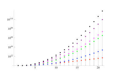
Figure 1: Factorials of Pisot numbers together with the standard factorial (red) versus $n$ for $q=(1-\sqrt{5})/2$ (blue), $q=(1-\sqrt{2})$ (green), $q=(3-\sqrt{5})/2$ (magenta), $q=(2-\sqrt{3}$ (purple), $q=(5-\sqrt{21})/2$ (black).

4 Moment measure for the symmetric deformation of integers

To a given $q>0$ let us associate the sequence $\left(x_{n}\right)_{n\in\mathbb{N}}$ defined by the symmetric deformations of nonnegative integers $(x_{n}\equiv{}^{[s]}[n]_{q})_{n\in\mathbb{N}}$ given by (3.27). Our aim is to make explicit the moment measure for this sequence, i.e. to find a probability distribution $t\mapsto w_{q}(t)$ on $[0,R)$ such that

$$x_{n}!={}^{[s]}[n]_{q}!=\int_{0}^{R}t^{n}\,w_{q}(t)\,dt\,.$$

Since

$$R=\lim_{n\to\infty}x_{n}=\infty\,,\quad\forall\ q>0\,,$$

its associated exponential

$$\mathfrak{e}_{q}(t)\equiv\mathcal{N}_{q}(t)=\sum_{n=0}^{+\infty}\frac{t^{n}}{x_{n}!}$$ (4.28)

defines an analytic entire function $\mathfrak{e}_{q}(z)$ in the complex plane for any positive $q$. This series coincides with $\mathcal{N}(t)$ (2.1) that now we call $\mathcal{N}_{q}(t)$ since $x_{n}$ depends on $q$.

Figure 2: $\mathfrak{e}_{q}(t)$ for $q=1$ (red), $q=(3-\sqrt{5})/2$ (blue), $q=2-\sqrt{3}$ (green), $q=(5-\sqrt{21})/2$ (purple).

Let us now introduce the “auxiliary” exponential :

$$\mathfrak{E}_{q}(t):=\sum_{n=0}^{\infty}q^{\frac{n(n+1)}{2}}\frac{t^{n}}{x_{n}!}\equiv\sum_{n=0}^{\infty}\frac{t^{n}}{y_{n}!}\,,$$

where $y_{n}:=q^{-n}x_{n}$. Its radius of convergence is $\infty$ for $0<q\leq 1$ and is equal to $1/(q-q^{-1})$ for $q>1$.

Figure 3: $\mathfrak{E}_{q}(t)$ for $q=1$ (red), $q=(3-\sqrt{5})/2$ (blue), $q=2-\sqrt{3}$ (green), $q=(5-\sqrt{21})/2$ (purple).

This last exponential is connected with the two standard $q$-exponentials as they are defined in [20] (see Appendix B for more details):

$$\mathfrak{E}_{q}(t)=e^{qt}_{q^{-2}}=E^{qt}_{q^{2}}\,,$$ (4.29)

where

$$e_{q}^{x}:=\sum_{n=0}^{\infty}\frac{x^{n}}{[n]_{q}!}\quad\left(=\frac{1}{\prod_{j=0}^{\infty}(1-q^{j}(1-q)x)}\quad\mbox{for}\quad q<1\right)\,,$$

$$E_{q}^{x}:=\sum_{n=0}^{\infty}q^{n(n-1)/2}\frac{x^{n}}{[n]_{q}!}=e_{q^{-1}}^{x}\quad\left(=\prod_{j=0}^{\infty}(1+q^{j}(1-q)x)\quad\mbox{for}\quad q<1\right)\,,$$ (4.30)

and

$$[n]_{q}:=\frac{1-q^{n}}{1-q}.$$

We note that the series $e_{q}^{x}$ converges for all $x$ if $q\geq 1$ and for all $x$ such that $|x|<1/(1-q)$ if $q<1$. On the contrary, $E_{q}^{x}$ converges for all $x$ if $q\leq 1$ and for all $x$ such that $|x|<1/(1-q^{-1})$ if $q>1$. From the relation $e_{q}^{-x}E_{q}^{x}=1$, valid for all $x$ such that $|x|<1/(1-q)$ if $q<1$ and for all $x$ such that $|x|<1/(1-q^{-1})$ if $q>1$, we infer that, in the case $q\leq 1$,

$$\left[\mathfrak{E}_{q}(t)\right]^{-1}=\mathfrak{E}_{q^{-1}}(-t)\quad\forall\,t\quad\mbox{such that}\quad|t|<\frac{1}{q^{-1}-q}\,.$$ (4.31)

Also note that due to (4.29) and (4.30), the expression of $\mathfrak{E}_{q}(t)$ as an infinite product for $q<1$ reads

$$\mathfrak{E}_{q}(t)=\prod_{j=0}^{\infty}(1+q^{2j+1}\,(1-q^{2})\,t)\quad\mbox{for}\quad|t|<\frac{1}{q(1-q^{2})}\,,$$

and so the first zero of $\mathfrak{E}_{q}(t)$ standing on the left of the origin is equal to $-1/(q(1-q^{2}))$. Due to these relations, the auxiliary exponential $\mathfrak{E}_{q}(t)$ is involved in the $q$-integral representation(s) of the $q$-gamma function $\Gamma_{q}(x)$ defined [20] by

$$\Gamma_{q}(x)=\frac{(1-q)_{q}^{x-1}}{(1-q)^{x-1}}\,,\quad x>0\,,$$

where the expression $(1+a)^{x}_{q}$ is given in Appendix B. It obeys the functional equation

$$\Gamma_{q}(x+1)=[x]_{q}\,\Gamma_{q}(x)\,,\quad\mbox{for all}\ x>0\,,\quad\Gamma_{q}(1)=1\,,$$

and so

$$\Gamma_{q^{2}}(x+1)=q^{x-1}\,{}^{[s]}[x]_{q}\,\Gamma_{q^{2}}(x)\,.$$ (4.32)

(a) $\Gamma_{q}(x)$                                                         (b) $\Gamma_{q^{2}}(x)$

Figure 4: Representations of $q$-gamma functions for $q=1$ (red), $q=(3-\sqrt{5})/2$ (blue), $q=2-\sqrt{3}$ (green), $q=(5-\sqrt{21})/2$ (purple).

A first integral representation is the following:

$$\Gamma_{q}(x)=\int_{0}^{\frac{1}{1-q}}t^{x-1}E_{q}^{-qt}\,d_{q}t\ .$$

The $q$–integral (introduced by Thomae [21] and Jackson [22]) is defined by

$$\int_{0}^{a}f(t)\;d_{q}t=(1-q)\sum_{j=0}^{\infty}a\;q^{j}\,f(a\;q^{j})\,,$$ (4.33)

and can be considered also as an ordinary integral with a discrete measure:

$$\int_{0}^{a}f(t)\;d_{q}t=\int_{0}^{\infty}\rho_{q}(t,a)f(t)\,dt\,,\qquad\rho_{q}(t,a)=(1-q)\sum_{j=0}^{\infty}aq^{j}\,\delta(t-aq^{j})\,.$$ (4.34)

Therefore, one derives from (4.33) and (4.34) the integral representation

$$\Gamma_{q}(x)=\int_{0}^{\infty}\rho_{q}(t,1/(1-q))\,t^{x-1}E_{q}^{-qt}\,dt\,.$$ (4.35)

Now, particularizing eq. (4.32) to nonnegative integer values $x=n$ we obtain the expression

$$\Gamma_{q^{2}}(n+1)=q^{\frac{n(n-1)}{2}}\,{}^{[s]}[n]_{q}\,\Gamma_{q^{2}}(n)=q^{-n}\,q^{\frac{n(n+1)}{2}}\,x_{n}!\,.$$ (4.36)

Combining (4.36) with (4.35), (4.29), and the integration variable change $t\mapsto q\;t$, we get the solution to the moment problem with a positive measure for the sequence $\left(q^{\frac{n(n+1)}{2}}\,x_{n}!\right)_{n\in\mathbb{N}}$ when $q<1$:

$$q^{\frac{n(n+1)}{2}}\,x_{n}!=\int_{0}^{\infty}t^{n}\,\varpi_{q}(t)\,dt\,,$$ (4.37)

where $\varpi_{q}(t)$ is the discrete measure:

$$\varpi_{q}(t)=\sum_{j=0}^{\infty}q^{2j}\,\,\mathfrak{E}_{q}\left(-\frac{q^{2j}}{q^{-1}-q}\right)\,\delta\left(t-\frac{q^{2j}}{q^{-1}-q}\right)\,.$$

An important point to be noted concerning this measure is its positiveness. Indeed, from (4.31) the factors $\mathfrak{E}_{q}\left(-\frac{q^{2j}}{q^{-1}-q}\right)$ are positive for all $j\geq 0$.

In order to solve the moment problem for the sole sequence $(x_{n}!)_{n\in\mathbb{N}}$ it is necessary to solve it for the sequence $\left(q^{-\frac{n(n+1)}{2}}\right)_{n\in\mathbb{N}}$ and to use an adapted composition formula [23] for moments: let $a(t)$ and $b(t)$ be two weight functions solving the moment problems

$$a_{n}!=\int_{0}^{\infty}t^{n}a(t)\,dt\,,\qquad b_{n}!=\int_{0}^{\infty}t^{n}b(t)\,dt\,,$$

respectively. Then the weight function defined by the (multiplicative) convolution

$$w(t):=\int_{0}^{\infty}a(t/u)\,b(u)\,\frac{du}{u}$$ (4.38)

solves the moment problem

$$a_{n}!\,b_{n}!=\int_{0}^{\infty}t^{n}w(t)\,dt\,.$$

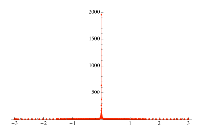
Figure 5: Representation of the function $g_{q}(t)$ for $q=(3-\sqrt{5})/2$.

Now, from [24] and [23] a positive measure solution to the moment problem for the sequence $\left(q^{-\frac{n(n+1)}{2}}\right)_{n\in\mathbb{N}}$, $0<q<1$, is given by

$$q^{-\frac{n(n+1)}{2}}=\int_{0}^{\infty}t^{n}g_{q}(t)\,dt\,,$$ (4.39)

with

$$g_{q}(t)=\frac{1}{\sqrt{2\pi\,|\ln{q}|}}\,\exp\left[-\frac{\left[\ln\left(\frac{t}{\sqrt{q}}\right)\right]^{2}}{2|\ln q|}\right]\,.$$

Finally, applying the composition formula (4.38) to the product of (4.37) and (4.39) yields the solution to the moment problem for the sequence $(x_{n}!)$:

$$x_{n}!=q^{-\frac{n(n+1)}{2}}\,q^{\frac{n(n+1)}{2}}\,x_{n}!=\int_{0}^{\infty}t^{n}w_{q}(t)\,dt\,$$

with the positive measure density given by

$$w_{q}(t)=\int_{0}^{\infty}g_{q}(t/u)\,\varpi_{q}(u)\,\frac{du}{u}=(q^{-1}-q)\sum_{j=0}^{\infty}\,g_{q}\left(t\,\frac{q^{-1}-q}{q^{2j}}\right)\mathfrak{E}_{q}\left(-\frac{q^{2j}}{q^{-1}-q}\right)\,.$$

5 CS quantization of the complex plane with integer symmetric deformations of the integer numbers

As was announced above, we fix our attention to Case 2 in Section 3 by considering the sequence of integers $\left(x_{n}={}^{[s]}[n]_{q}\right)$ defined for $n\geq 0$ by (3.27) where $q$ ($0<q<1$) is solution of eq. (3.26), i.e, $X^{2}-sX+1=0$ with integer $s\geq 3$. From (3.25) these integers $x_{n}$ obey the recurrence relation

$$x_{n+1}-sx_{n}+x_{n-1}=0\,,\quad x_{0}=0\,,\quad x_{1}=1\,.$$

In section 4 we have solved the moment problem for the sequence $(x_{n}!)_{n\in\mathbb{N}}$, so we can construct a family of CS associated to $(x_{n})_{n\in\mathbb{N}}$ according to (2.4) and solving the identity according to ((v)). We now proceed with numerical explorations by choosing the lowest cases $s=3,4$ and $5$ which correspond to $q=(3-\sqrt{5})/2,\;q=2-\sqrt{3}$ and $q=(5-\sqrt{21})/2$ respectively. Note that $(3-\sqrt{5})/2=1/\tau^{2}$, where $\tau=(1+\sqrt{5})/2$ is the golden mean. These $q$-numbers ($q=(3-\sqrt{5})/2$) are Fibonacci numbers which occupy the odd place in the Fibonacci series (see Table 1). The limit of ${}^{s}[n]_{q}$ (3.27) when $q\to 1$ is $n$.

The explicit expression of the coherent states (2.4) associated to these $q$-integers ${}^{[s]}[n]_{q}$ is

$$|v_{z}\rangle_{q}=\sum_{n=0}^{\infty}\frac{1}{\sqrt{\mathcal{N}_{q}(|z|^{2})}}\frac{z^{n}}{\sqrt{{}^{[s]}[n]_{q}!}}\,|e_{n}\rangle\,.$$

The CS $|v_{z}\rangle_{q}$ in the limit $q\to 1$ goes to the standard CS $|v_{z}\rangle$ [25, 14, 26]

$$|v_{z}\rangle=\sum_{n=0}^{\infty}\frac{1}{\sqrt{\exp(|z|^{2})}}\frac{z^{n}}{\sqrt{n!}}\,|e_{n}\rangle\,$$ (5.40)

(for which the kets $|e_{n}\rangle$ are given their usual Fock interpretation of number states, i.e. $|e_{n}\rangle\equiv|n\rangle$), taking into account that when $q$ goes to $1$ ${}^{[s]}[n]_{q}\to n$ and $\mathcal{N}_{q}(|z|^{2})\to\exp{(|z|^{2})}$.

In the following we study the physical properties of these $q$-CS for different values of $q$ and we compare with the standard CS. A graphical way to see this limit is to consider the ratio-function

$$d_{q}(n)=\frac{{}^{[s]}[n]_{q}!}{n!}$$

and display it versus $n$ for different values of $q$ [2] (see Fig. 6a). Also in figure 6b we represent the normalization function $\mathcal{N}_{q}(t)$ (4.28) of the CS versus $t$ for positive values of $t$ and different values of $q$.

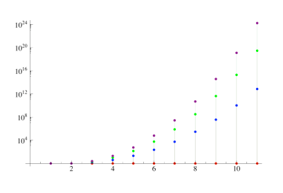
(a) $d_{q}(n)$                                                           (b) $\mathcal{N}_{q}(t)$

Figure 6: Representation of $d_{q}(n))$ and $\mathcal{N}_{q}(t)$ with $t\geq 0$ for $q=1$ (red), $(3-\sqrt{5})/2$ (blue), $2-\sqrt{3}$ (green), $(5-\sqrt{21})/2$ (purple).

Let us suppose that the state $|e_{n}\rangle$ corresponds to the state of $n$ bosons $|n\rangle$. Then the probability of finding $n$ bosons in the $q$-CS $|v_{z}\rangle_{q}$ is given by the $q$-Poisson distribution

$$\rho_{q}(n,|z|)=\dfrac{|z|^{2n}}{\mathcal{N}(|z|^{2})\;x_{n}!},$$

whose limit when $q\to 1$ is the standard Poisson distribution appearing in the standard CS. In figures 7 we display the $q$-Poisson distribution for different values of $|z|$ and $q$. In particular, in figure 7b we also display the standard Poisson distribution (in yellow) and notice that the $q$-Poisson distributions are left displaced with respect to the standard Poisson distribution. It shows that $\rho_{q}(n,|z|)$ is a sub-Poissonian distribution. The Mandel parameter [27]

$$Q_{q}(|z|^{2})=\frac{(\Delta X_{N})^{2}-\langle X_{N}\rangle}{\langle X_{N}\rangle}=\frac{\langle X_{N}^{2}\rangle-\langle X_{N}\rangle^{2}-\langle X_{N}\rangle}{\langle X_{N}\rangle}$$

measures the deviation of a Poisson-like distribution from the Poisson distribution. The Mandel parameter for the Poisson distribution vanishes since for standard CS $(\Delta N)^{2}=\langle N\rangle$, where $N$ is the number operator; if $Q_{q}(|z|^{2})<0$ we have a sub-Poissonian distribution, i.e. there is an antibunching effect; finally if $Q_{q}(|z|^{2})>0$ the $q$-Poisson distribution is a super-Poissonian distribution, i.e. the bunching effect appears. For our $q$-CS the Mandel parameter is negative (see Fig. 8).

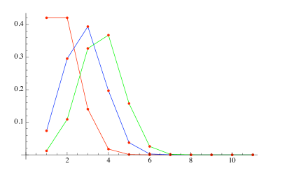
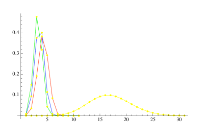
(a) $|z|=4$ (red), $5$ (blue), $6$ (green) and $q=(3-\sqrt{5})/2$.    (b) $|z|=4,\;q=1$ (yellow), $(3-\sqrt{5})/2$ (red),
.   $2-\sqrt{3}$ (blue), $(5-\sqrt{21})/2$ (green).

Figure 7: Representations of Poisson-like distributions $\rho_{q}(n,|z|)$ versus $n$ for different values of the parameters $|z|$ and $q$.

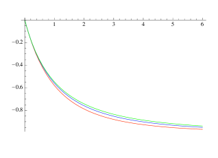
Figure 8: The Mandel parameter $Q_{q}(|z|^{2})$ versus $|z|$ for $q=(3-\sqrt{5})/2$ (red), $2-\sqrt{3}$ (blue), $(5-\sqrt{21})/2$ (green).

Expression (2.14) shows us that these $q$-CS are intelligent states for the operators $Q$ and $P$ (2.11). The variances of $Q$ and $P$ read respectively:

$$(\Delta_{v_{z}}Q)^{2}=(\Delta_{v_{z}}P)^{2}=\frac{1}{2}|\langle v_{z}|[Q,P]|v_{z}\rangle|=\frac{1}{2}\left|\frac{1}{\mathcal{N}(|z|^{2})}+(s-1)|z|^{2}-|z|^{4}\left\langle\frac{1}{x_{n+2}}\right\rangle\right|\,.$$

This quantity is $\geq 1/2$ for all $z\in\mathbb{C}$ since $x_{N+1}-x_{N}(=(s-1)x_{N}-x_{N-1})\geq I_{d}$. Only for $z=0$, i.e. for the vacuum state $|v_{0}\rangle=|e_{0}\rangle$, we have:

$$(\Delta_{v_{0}}Q)^{2}=(\Delta_{v_{0}}P)^{2}=\frac{1}{2}|\langle v_{0}|[Q,P]|v_{0}\rangle|=1/2\,.$$

So, these operators have no minimum-uncertainty state in the sense of ordinary quantum mechanics, at the exception of the vacuum, in such a way that the vacuum uncertainty product provides a global lower bound (see Fig. 9). According to these results squeezing does not occur in $|v_{z}\rangle_{q}$ for any $q$ and $z$.

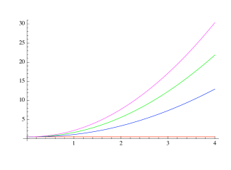
Figure 9: $(\Delta_{v_{z}}Q)^{2}$ versus $|z|$ for $q=1$ (red), $(3-\sqrt{5})/2$ (blue), $2-\sqrt{3}$ (green), $(5-\sqrt{21})/2$ (purple).

The $q$-deformed boson creation and annihilation operators ($a,\,a^{\dagger}$) (2.9) and (2.10) can be related to the standard boson creation and annihilation operators ($b,\;b^{\dagger}$) by

$$a^{\dagger}=\sqrt{\frac{x_{n+1}}{n+1}}\;b^{\dagger},\qquad a=\sqrt{\frac{x_{n}}{n}}\;b.$$

Thus, standard $n$-boson states $|e_{n}\rangle$ can be rewritten as $n$-$q$-deformed-boson states as

$$|e_{n}\rangle=\frac{1}{\sqrt{n!}}(b^{\dagger})^{n}|e_{0}\rangle=\frac{1}{\sqrt{x_{n}!}}(a^{\dagger})^{n}|e_{0}\rangle.$$

Hence, the $q$-CS $|v_{z}\rangle$ can also expressed in terms of $n$-bosons operators by

$$|v_{z}\rangle=\sum_{n=0}^{\infty}\frac{1}{\sqrt{\mathcal{N}(|z|^{2})}}\frac{z^{n}}{{x_{n}!}}\,(a^{\dagger})^{n}|e_{0}\rangle\,=\sum_{n=0}^{\infty}\frac{1}{\sqrt{\mathcal{N}(|z|^{2})}}\frac{z^{n}}{\sqrt{x_{n}!\;n!}}\,(b^{\dagger})^{n}|e_{0}\rangle\,.$$

We can compare the properties of the $q$-CS with those of the standard CS by using the characteristic functional [29] (see Fig. 10)

$$\rho_{q}(n)=\frac{{}^{[s]}[n+1]_{q}/^{[s]}[n]_{q}}{(n+1)/n}$$

Obviously, in our case, $\rho_{q}(n)>1$ for any $q$ (see Fig. 10).

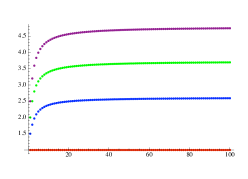
Figure 10: Characteristic functional for $q=1$ (red), $(3-\sqrt{5})/2$ (blue), $2-\sqrt{3}$ (green), $(5-\sqrt{21})/2$ (purple).

Signal-to-quantum noise ratio for these $q$-deformed photons is determined by the relation

$$\sigma_{q}=\frac{\langle Q\rangle_{q}^{2}}{(\Delta Q)_{q}^{2}}.$$

Note that $\langle Q\rangle_{q}=\sqrt{2}\Re z$. Fig. 11 shows that the signal-to-quantum noise ratio for $q$-deformed photons is not enhanced over the standard photon case (in red).

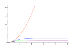
Figure 11: Signal-to-quantum noise ratio versus $|z|$ for $q=1$ (red), $(3-\sqrt{5})/2$ (blue), $2-\sqrt{3}$ (green), $(5-\sqrt{21})/2$ (purple).

In relation with the $q$-Pisot coherent state quantization of angle (angle operator $A_{\theta}$ (2.8)) we display (Figs. 12, 13 and 14) the lower symbol of $A_{\theta}$ ($\check{\theta}(z,\bar{z})$) whose explicit expression is given by (2.18). In order to make comparisons we also display in some of these figures the angle lower-symbol for the standard coherent states (5.40). We easily check that the function $\check{\theta}(z,\bar{z})$ tends to the classical angle function as $|z|\to\infty$. Effectively, it is enough to se that the function $d_{k}(r)$ goes to 1 when $r=|z|=r$ goes to $\infty$ (and $q=1$) (see Fig. 15 and 16).

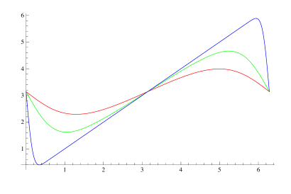
(a) Standard coherent states.                           (b) $q$-Pisot coherent states ($q=(3-\sqrt{5})/2$).

Figure 12: Lower symbol of the angle operator for different values of the parameters $|z|=0.5$ (red), $1$ (green), $5$ (blue) and $\theta\in[0,2\pi)$.

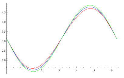
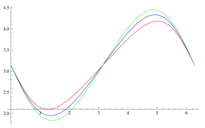
(a) $|z|=0.5$.                                                         (b) $|z|=2$.

Figure 13: Lower symbol of the angle operator for $q=(3-\sqrt{5})/2$ (red), $2-\sqrt{3}$ (blue), $(5-\sqrt{21})/2$ (green) and $\theta\in[0,2\pi)$..

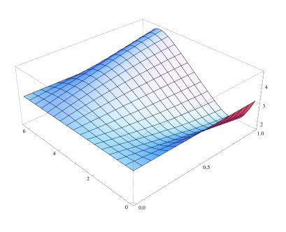
(a) Standard coherent states.              (b) $q$-Pisot coherent states ($q=(3-\sqrt{5})/2$).

Figure 14: Lower symbol of the angle operator for $|z|\in[0,1]$ and $\theta\in[0,2\pi)$.

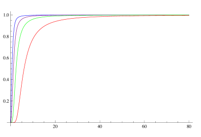
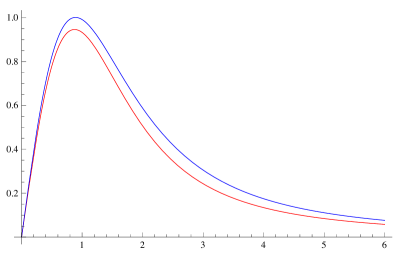
(a) $k=1$ (blue), $k=2$ (purple), $k=4$ (green),              (b): $k=1$; $q=(3-\sqrt{5})/2$ (blue), $q=2-\sqrt{3}$ $k=10$ (red).                                                                   (red).

Figure 15: Representation of the function $d_{k}(r)$ (2.17): (a) for $q=1$ and (b) for $q\neq 1$.

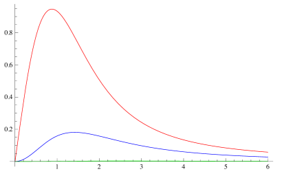
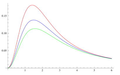
(a) $k=1$ (red), $k=2$ (blue), $k=4$ (green)              (b): $k=2$; $q=(3-\sqrt{5})/2$ (red), $q=2-\sqrt{3}$ (blue) and $q=(3-\sqrt{5})/2$.                                                  and $q=(5-\sqrt{21})/2$ (red).

Figure 16: Representation of the function $d_{k}(r)$ (2.17) for $q\neq 1$.

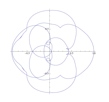
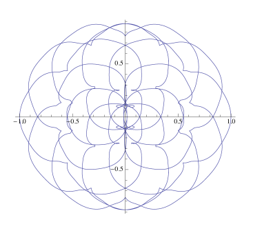
(a) $q=(3-\sqrt{5})/2$.                                            (b) $q=2-\sqrt{3}$.

Figure 17: Plots of $\Im\check{z}\left(t\right)$ versus $\Re\check{z}\left(t\right)$ for different values of $q$ and $0\leq t\leq 8\pi$.

(a) $q=(5-\sqrt{21})/2$.                                            (b)

Figure 18: Plots of $\Im\check{z}\left(t\right)$ versus $\Re\check{z}\left(t\right)$ for different values of $q$ and $0\leq t\leq 8\pi$. In Fig. 18(b) we plot the previous three figures together with the corresponding to $q=1$ which is a circle of radius 1.

Another domain of interest is the behavior of the $q$-Pisot coherent states in phase space. For this purpose we firstly study the trajectories in phase space, i.e., the time evolution of $a=A_{z}$ (2.9), i.e. $A_{z}(t)=e^{-i\hat{H}t}\,A_{z}\,e^{i\hat{H}t}$, corresponding to the classical phase space point $z=(\mathbf{q}+i\mathbf{p})/\sqrt{2}$, which is given by the mean value in coherent states $|v_{z}\rangle$, $\check{z}\left(t\right)=\left\langle v_{z}\right|A_{z}(t)\left|v_{z}\right\rangle$ (2.20). In Figs. 17 and 18 we plot $\Im\check{z}\left(t\right)$ versus $\Re\check{z}\left(t\right)$ for different values of $q$ and $0\leq t\leq 8\pi$. Note that since the $q$ numbers involved in these CS are integers the phase space trajectories are periodic with period $2\pi$. We show the phase space distribution $\rho_{v_{z_{0}}}(z)$ (2.21) in Fig. 19 with the fixed state $|v_{(1,1)}\rangle$ and in Fig. 20 for the initial CS state $z_{0}=(1,0)$ and different values of $q$.

(a) Standard coherent states.                       (b) $q$-Pisot coherent states ($q=(3-\sqrt{5})/2$).

Figure 19: Phase space distribution $\rho_{v_{z_{0}}}(z)$ for the particular state $|v_{z_{0}}\rangle$ with $z_{0}=(1,1)$. The black circle corresponds to the expected phase space given by (2.20).

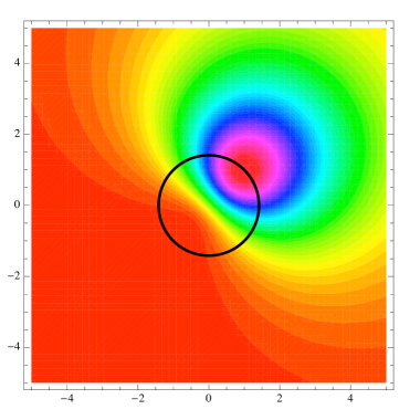
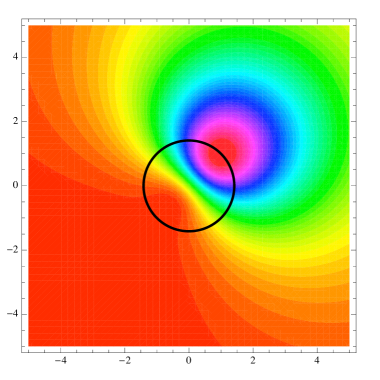
(a) $q$-Pisot coherent states ($q=2-\sqrt{3}$)             (b) $q$-Pisot coherent states ($q=(5-\sqrt{21})/2)$.

Figure 20: Phase space distribution $\rho_{v_{z_{0}}}(z)$ for the particular state $|v_{z_{0}}\rangle$ with $z_{0}=(1,0)$. The black circle corresponds to the expected phase space given by (2.20).

6 Conclusions

In this paper we have introduced a $q$-dependent family of coherent states and we have explored some properties of the quantum harmonic oscillator obtained through the corresponding coherent state quantization. We have restricted our study to the case in which $q^{-1}$ is a quadratic unit Pisot number, since then the spectrum of the quantum Hamiltonian is made of the $q$-deformed integers ${}^{[s]}[n]_{q}=\frac{q^{n}-q^{-n}}{q-q^{-1}}$ which are still integers and form sequences of Fibonacci type. We have put into evidence interesting quantum features issued from these particular algebraic cases, concerning particularly the localization in the configuration space and in the phase space, probability distributions and related statistical features, time evolution and semi-classical phase space trajectories. The periodicity of the latter nicely reflects the algebraic Pisot nature of the deformation parameter $q$. By contrast we present the semi-classical phase space trajectories for irrational values of $q$ (Figs. 21 and Fig. 22). Obviously, the trajectories are not periodic.

Let us place the present study into a more general perspective. “Coherent state(s) quantization” [7] is a generic phrase for naming a certain point of view in analyzing a set $X$ (here the complex plane) of parameters, equipped with a measure $\mu$ (here $w_{q}(|z|^{2})\,d^{2}z/\pi$). The approach matches what physicists understand by quantization when the “observed” measure space $X$ has a phase space or symplectic structure (it is not exactly the case here since the measure is not the usual symplectic one). It matches also well established approaches by signal analysts, like wavelet analysis [32]. The set $X$ can be finite, countably infinite or uncountably infinite. The approach is generically simple, of Hilbertian essence, and always the same: one starts from the Hilbert space $L^{2}(X,\mu)$ of complex square integrable functions on $X$ with respect to the measure $\mu$. One chooses an orthonormal set $\mathcal{O}$ of vectors $\phi_{n}$ in it (here $\phi_{n}(x)=\bar{x}^{n}/x_{n}!$ satisfying the finiteness condition $\mathcal{N}(x)=\sum_{n}|\phi_{n}(x)|^{2}<\infty$, and a “companion” Hilbert space $\mathcal{H}$ (the space of “quantum states”) with orthonormal basis (here the $|e_{n}\rangle$’s) in one-to-one correspondence with the elements of $\mathcal{O}$. There results a family $\mathcal{C}$ of states

$$|x\rangle=\frac{1}{\sqrt{\mathcal{N}(x)}}\sum_{n}\overline{\phi_{n}(x)}\,|e_{n}\rangle$$

(the “coherent states”) in $\mathcal{H}$, which are labelled by elements of $X$ and which resolve the unity operator in $\mathcal{H}$. This is the departure point for analysing the original set and functions living on it from the point of view of the frame (in its true sense) $\mathcal{C}$. We end in general with a non-commutative algebra of operators in $\mathcal{H}$, set aside the usual questions of domains in the infinite dimensional case.

There is a kind of manifest universality in this approach. The change of the frame family $\mathcal{C}$ produces another quantization, another point of view, possibly equivalent to the previous one, possibly not. The present study lies in the continuity of a series of such explorations, which were already present in the first works by Klauder at the beginning of the sixties of the past century (see for instance [16, 33] and references therein), pursued by Berezin [15] in his famous paper of 1975, and more recently extended to various measure sets (see for instance [34, 35, 36, 37, 38, 39]).

That this correspondence fits the CS quantization is once more the mark of the universality and the easy implementation of this type of analysis, in comparison with usual quantization methods (see the review [40]).

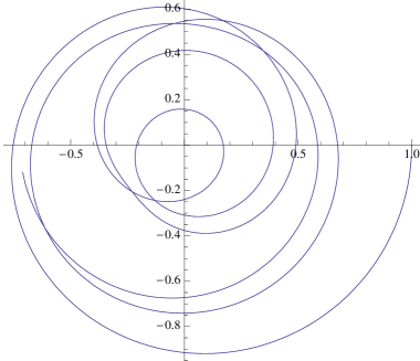
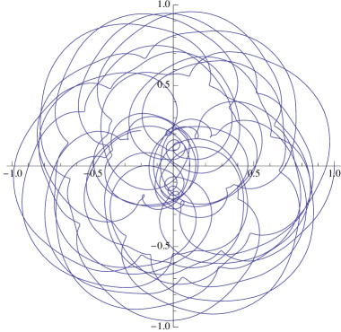
(a) $q=\sqrt{2}$.                                            (b) $q=e$.

Figure 21: Plots of $\Im\check{z}\left(t\right)$ versus $\Re\check{z}\left(t\right)$ for irrational values of $q$ and $0\leq t\leq 8\pi$.

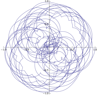
(a) $q=\pi$.                                            (b)

Figure 22: Plots of ${\Im}\check{z}\left(t\right)$ versus $\Re\check{z}\left(t\right)$ for irrational values of $q$ and $0\leq t\leq 8\pi$. In Fig. 22(b) we plot the previous three figures together with the corresponding to $q=1$ for $0\leq t\leq 2\pi$.

Appendix

A   Inequalities

Let us consider the Hilbert space $L^{2}([0,R),w(t)dt)$ of square integrable functions on the interval $[0,R)\subset\mathbb{R}$ with respect the measure $w(t)\;dt$. Scalar product and norms are respectively defined by

$$\langle f_{1}|f_{2}\rangle=\int_{0}^{R}\overline{f_{1}}(t)\,f_{2}(t)\,w(t)\,dt\,,\qquad\|f\|=\sqrt{\int_{0}^{R}|f(t)|^{2}\,w(t)\,dt}\,.$$

In particular for the monomial functions $m_{\alpha}(t):=t^{\alpha}$,

$$\left\|m_{\frac{n}{2}}\right\|^{2}=\int_{0}^{R}t^{n}\,w(t)\,dt=x_{n}!\,.$$

From the Cauchy-Schwarz inequality, $|\langle f_{1}|f_{2}\rangle|\leq\|f_{1}\|\,\|f_{2}\|$ valid for any pair $f_{1},f_{2},$ in $L^{2}([0,R),w(t)dt)$ we infer the inequality:

$$x_{\frac{n_{1}+n_{2}}{2}}!=\int_{0}^{R}t^{\frac{n_{1}+n_{2}}{2}}\,w(t)\,dt=\left\langle m_{\frac{n_{1}}{2}}|m_{\frac{n_{2}}{2}}\right\rangle\leq\left\|m_{\frac{n_{1}}{2}}\right\|\,\cdot\left\|m_{\frac{n_{2}}{2}}\right\|=\sqrt{x_{n_{1}}!\,x_{n_{2}}!}\,,$$ (0.41)

for any $n_{1},n_{2}\in\mathbb{N}$, actually for any $n_{1},n_{2}\in\mathbb{R}^{+}$.

Now, consider the series defined for $k\in\mathbb{N}$ and for $t\geq 0$ by:

$$\mathcal{S}_{k}(t)=\frac{1}{\mathcal{N}(t)}\sum_{n=0}^{\infty}\frac{x_{\frac{k}{2}+n}!}{x_{n}!x_{n+k}!}\,t^{n+k/2}\,.$$

Due to (0.41) we have a first upper bound:

$$\mathcal{S}_{k}(t)=\frac{1}{\mathcal{N}(t)}\sum_{n=0}^{\infty}\frac{x_{\frac{k}{2}+n}!}{\sqrt{x_{n}!x_{n+k}!}}\,\frac{1}{\sqrt{x_{n}!x_{n+k}!}}\,t^{n+k/2}\leq\frac{1}{\mathcal{N}(t)}\sum_{n=0}^{\infty}\frac{1}{\sqrt{x_{n}!x_{n+k}!}}\,t^{n+k/2}\,.$$

Let us apply again the Cauchy-Schwarz inequality:

$$\sum_{n=0}^{\infty}\frac{1}{\sqrt{x_{n}!x_{n+k}!}}\,t^{n+k/2}\leq\sqrt{\sum_{n=0}^{\infty}\frac{1}{x_{n}!}\,t^{n}}\,\sqrt{\sum_{n=0}^{\infty}\frac{1}{x_{n+k}!}\,t^{n+k}}\leq\mathcal{N}(t)\,.$$

In consequence, we can assert that

$$\mathcal{S}_{k}(t)\leq 1\qquad\forall\ k\geq 0\,,\,t\geq 0\,.$$

B   Standard $q$-calculus

There exists a large literature [21, 28, 41, 42, 43, 44], devoted to $q$-calculus in the standard sense (see specially [20] for updated results), which means that the $q$-deformation of a number $x$ is given by the asymmetric expression

$$[x]_{q}:=\frac{1-q^{x}}{1-q}\,.$$

Suppose here and further that $0<q<1$ and let us adopt the following notations for the related infinite products

$$(a+b)_{q}^{n} = \prod_{j=0}^{n-1}(a+q^{j}b)\ ,\quad\text{ if }n\in\mathbb{Z}^{+}\ ,$$ (0.42)

$$(1+a)_{q}^{\infty} = \prod_{j=0}^{\infty}(1+q^{j}a)\ ,$$ (0.43)

$$(1+a)_{q}^{t} = \frac{(1+a)_{q}^{\infty}}{(1+q^{t}a)_{q}^{\infty}}\ ,\quad\text{ if }t\in\mathbb{C}\ .$$ (0.44)

Under the assumptions on $q$, the infinite product (0.43) is convergent, and the definitions (0.42) and (0.44) are consistent.

The $q$–gamma function $\Gamma_{q}(t)$, a $q$–analogue of Euler’s gamma function, was introduced by Thomae [21] and later by Jackson [28] as the infinite product

$$\Gamma_{q}(t)=\frac{(1-q)_{q}^{t-1}}{(1-q)^{t-1}}\ ,\quad t>0\ .$$

A first integral representation of $\Gamma_{q}(t)$ reads as

$$\Gamma_{q}(t)=\int_{0}^{\frac{1}{1-q}}x^{t-1}E_{q}^{-qx}d_{q}x\ .$$ (0.45)

Here in (0.45) $E_{q}^{x}$ is one of the two $q$–analogues of the exponential function,

$$E_{q}^{x} = \sum_{n=0}^{\infty}q^{n(n-1)/2}\frac{x^{n}}{[n]!}\ =\ (1+(1-q)x)_{q}^{\infty}\ ,$$ (0.46)

$$e_{q}^{x} = \sum_{n=0}^{\infty}\frac{x^{n}}{[n]!}\ =\ \frac{1}{(1-(1-q)x)_{q}^{\infty}}\ ,$$ (0.47)

and the $q$–integral (introduced by Thomae [21] and Jackson [22]) is defined by

$$\int_{0}^{a}\;f(x)\;d_{q}x=(1-q)\sum_{j=0}^{\infty}a\;q^{j}f(a\;q^{j})\ .$$ (0.48)

Notice that the series on the right–hand side of (0.48) is guaranteed to be convergent as soon as the function $f$ is such that, for some $C>0,\ \alpha>-1$, $|f(x)|<Cx^{\alpha}$ in a right neighborhood of $x=0$. Also note that the $q$–exponential functions (0.46)-(0.47) are related by

$$e_{q}^{x}\;E_{q}^{-x}=E_{q}^{x}\;e_{q}^{-x}=1\,,$$

and that for $q\in(0,1)$ the series expansion of $e_{q}^{x}$ has radius of convergence $1/(1-q)$, whereas the series expansion of $E_{q}^{x}$ converges for every $x$.

The $q$–derivative $D_{q}$ of a function is defined by

$$(D_{q}f)(x)=\frac{f(qx)-f(x)}{(q-1)x}\ .$$

Jackson integral and $q$–derivative are related by the “fundamental theorem of quantum calculus” [30, p. 73], i.e.

Theorem 1

• If $F$ is any anti $q$–derivative of the function $f$, namely $D_{q}F=f$, continuous at $x=0$, then

  $$\int_{0}^{a}f(x)d_{q}x=F(a)-F(0)\ .$$

• For any function $f$ one has

  $$D_{q}\int_{0}^{x}f(t)d_{q}t=f(x)\ .$$

The $q$–analogue of the Leibniz rule is, as it is easy to check,

$$D_{q}(f(x)g(x))=g(x)D_{q}f(x)+f(qx)D_{q}g(x)\ .$$ (0.49)

An immediate consequence is the $q$–analogue of the rule of integration by parts:

$$\int_{0}^{a}g(x)D_{q}f(x)d_{q}x=f(x)g(x)\Big{|}_{0}^{a}-\int_{0}^{a}f(qx)D_{q}g(x)d_{q}x\ .$$

The Jackson integral in a generic interval $[a,b]$ is defined by [22]:

$$\int_{a}^{b}f(x)d_{q}x=\int_{0}^{b}f(x)d_{q}x-\int_{0}^{a}f(x)d_{q}x\ .$$

Improper integrals are also defined in the following way [22], [31]:

$$\int_{0}^{\infty/A}f(x)d_{q}x=(1-q)\sum_{n\in\mathbb{Z}}\frac{q^{n}}{A}f\Big{(}\frac{q^{n}}{A}\Big{)}\ .$$ (0.50)

Notice that in order the series on the right–hand side of (0.50) to be convergent, it suffices that the function $f$ satisfies the conditions: $|f(x)|<Cx^{\alpha},\quad\forall x\in[0,\epsilon)$, for some $C>0,\ \alpha>-1,\ \epsilon>0$; and $|f(x)|<Dx^{\beta},\quad\forall x\in[N,\infty)$, for some $D>0,\ \beta<-1,\ N>0$. In general though, even when these conditions are satisfied, the value of the sum will be dependent on the constant $A$. In order the integral to be independent of $A$, the anti $q$–derivative of $f$ needs to have limits for $x\rightarrow 0$ and $x\rightarrow+\infty$.

The $q$–exponential functions (0.46)-(0.47) satisfy the following properties:

1. $D_{q}e_{q}^{x}=e_{q}^{x}\ ,\qquad D_{q}E_{q}^{x}=E_{q}^{qx}$.

2. $e_{q}^{x}\;E_{q}^{-x}=E_{q}^{x}\;e_{q}^{-x}=1$.

3. $e_{q}^{x}=E_{1/q}^{x}$.

The function $\Gamma_{q}(t)$ is the “correct” $q$–analogue of the $\Gamma$–function, since it reduces to $\Gamma(t)$ in the limit $q\rightarrow 1$, and it satisfies a property analogue to $\Gamma(t+1)=t\,\Gamma(t)$. Indeed, $\Gamma_{q}(t)$ is equivalently expressed as

$$\Gamma_{q}(t)=\frac{(1-q)_{q}^{t-1}}{(1-q)^{t-1}}\ ,$$

and, in particular, it verifies

$$\Gamma_{q}(t+1)=[t]\;\Gamma_{q}(t)\ ,\quad\forall t>0\ ,\qquad\Gamma_{q}(1)=1\ .$$

C   The essential of symmetric $q$-calculus

We now recall the essential of the $q$-calculus in the symmetric case, i.e. when the $q$-deformation of a number, say $t$, is given by

$${}^{[s]}[t]_{q}=\frac{q^{t}-q^{-t}}{q-q^{-1}}\,.$$

To simplify, we will drop the subscript $q$ in all symbols when it is not really needed for the understanding.

$q$-derivative :

the symmetric $q$-derivative is defined as

$${}^{[s]}D_{q}f(x)=\frac{f(qx)-f(q^{-1}x)}{(q-q^{-1})x}\,.$$

Applied to a power of the variable $x$, it gives:

$${}^{[s]}D_{q}x^{n}={}^{[s]}[n]_{q}x^{n-1}\,.$$

The Leibnitz formula (0.49) reads in the present context:

$${}^{[s]}D_{q}(f(x)g(x))=f(q^{-1}x){}^{[s]}D_{q}g(x)+g(qx){}^{[s]}D_{q}f(x)\,.$$

“Proper” definite $q$-integral :

$$\int_{0}^{a}f(x)\,{}^{[s]}d_{q}x=(1-q^{2})a\sum_{n=0}^{\infty}q^{2n}f(q^{2n+1}a)\,.$$ (0.51)

Applied to a power of the variable $x$, it gives:

$$\int_{0}^{a}x^{n}\,{}^{[s]}d_{q}x=\frac{1}{{}^{[s]}[n+1]_{q}}a^{n+1}\,.$$

If a $q$-primitive $F(x)$ of $f(x)$ is known (i.e. $f(x)={}^{[s]}D_{q}F(x)$), then the integral (0.51) is, as expected, equal to

$$\int_{0}^{a}f(x)\,{}^{[s]}d_{q}x=F(a)-F(0)\,.$$

“Improper” definite $q$-integral :

$$\int_{0}^{\infty/A}f(x)\,{}^{[s]}d_{q}x=(1-q^{2})\sum_{n\in\mathbb{Z}}\frac{q^{2n}}{A}f\left(\frac{q^{2n+1}}{A}\right)\,.$$

If $f(x)={}^{[s]}D_{q}F(x)$, then this integral is equal to

$$\int_{0}^{\infty/A}f(x)\,{}^{[s]}d_{q}x=\underset{N\to\infty}{\lim}\left(F\left(\frac{q^{-2N}}{A}\right)-F\left(\frac{q^{2N}}{A}\right)\right)\,.$$

Factorials and $q$-exponentials :

the (symmetric) $q$-factorial is defined by

$${}^{[s]}[n]_{q}!={}^{[s]}[n]_{q}\times{}^{[s]}[n-1]_{q}\times\cdots\times{}^{[s]}[2]\times 1\,.$$

In the context of $q$-deformations, there exist two types of $q$-exponentials:

$$\mathfrak{e}_{q}(x) =\sum_{n=0}^{\infty}\frac{x^{n}}{{}^{[s]}[n]_{q}!}\,,$$

$$\mathfrak{E}_{q}(x) =\sum_{n=0}^{\infty}q^{\frac{n(n+1)}{2}}\frac{x^{n}}{{}^{[s]}[n]_{q}!}\,.$$

First we note that the symmetries

$$\mathfrak{e}_{1/q}(x)=\mathfrak{e}_{q}(x)\,,\qquad\mathfrak{E}_{1/q}(x)=1/\mathfrak{E}_{q}(-x)\,.$$

These two series obey the $q$-differential equations:

$${}^{[s]}D_{q}\,\mathfrak{e}_{q}(x)=\mathfrak{e}_{q}(x)\,,\qquad{}^{[s]}D_{q}\,\mathfrak{E}_{q}(x)=\mathfrak{E}_{q}(qx)\,.$$

$q$–Gamma function :

we define a gamma-type function through the proper definite integral:

$${}^{[s]}\widetilde{\gamma}_{q}(t)=\int_{0}^{\frac{1}{1-q^{2}}}x^{t-1}\,\mathfrak{E}_{q}(-qx)\,{}^{[s]}d_{q}x\,.$$

By performing an integration by parts, we can prove the following recurrence relation:

$${}^{[s]}\widetilde{\gamma}_{q}(t+1)=q^{t}\,{}^{[s]}[t]\,{}^{[s]}\widetilde{\gamma}_{q}(t)\,.$$

In particular, for $t=n\in\mathbb{N}$, we get:

$${}^{[s]}\widetilde{\gamma}_{q}(n+1)=q^{\frac{n(n+1)}{2}}\,{}^{[s]}[n]!\,.$$

D   Equation and solutions for general quadratic Pisot numbers

We consider two cases:

D.1   Positive conjugate case

Equation:

$$X^{2}-(a+1)X+(a-b)=0;\qquad a,b\in\mathbb{Z},\;\;a\geq b+1,\;\;b>0.$$

Solutions:

$$\begin{array}[]{l}1<a<\beta=\frac{1}{2}\left(a+1+\sqrt{(a-1)^{2}+4b}\right),\\[8.5359pt] 0<\beta^{\prime}=\frac{1}{2}\left(a+1-\sqrt{(a-1)^{2}+4b}\right)<1,\end{array}$$

with

$$\lfloor\beta\rfloor=a,\qquad\beta\beta^{\prime}=a-b\geq 1,\qquad\beta+\beta^{\prime}=a+1.$$

D.2   Negative conjugate case

Equation:

$$X^{2}-cX-d=0;\qquad c,d\in\mathbb{Z},\;\;c\geq d\geq 1.$$

Solutions:

$$1\leq c<\beta=\frac{1}{2}\left(c+\sqrt{c^{2}+4d}\right),\qquad-1<\beta^{\prime}=\frac{1}{2}\left(c-\sqrt{c^{2}+4d}\right)<0,$$

with

$$\lfloor\beta\rfloor=c,\qquad\beta\beta^{\prime}=-d\geq 1,\qquad\beta+\beta^{\prime}=c.$$

E   Powers and recurrence for general quadratic Pisot numbers

E.1   Positive conjugate case

$$\beta^{n}=v_{n}\beta+w_{n},\quad v_{0}=0,\;\;w_{0}=1,\quad v_{1}=1,\;\;w_{1}=0.$$

$$w_{n+1}=(b-a)v_{n},\ v_{n+1}=(a+1)v_{n}+(b-a)v_{n-1}.$$

$$v_{n}=\frac{\beta^{n}-\beta^{\prime n}}{\beta-\beta^{\prime}}$$

$$\beta^{n}+\beta^{\prime n}=(a+1)v_{n}+2(b-a)v_{n-1}.$$

E.1   Negative conjugate case

$$\beta^{n}=v_{n}\beta+w_{n},\ v_{0}=0,\ w_{0}=1,v_{1}=1,\ w_{1}=0.$$

$$w_{n+1}=dv_{n},\ v_{n+1}=cv_{n}+dv_{n-1}.$$

$$v_{n}=\frac{\beta^{n}-\beta^{\prime n}}{\beta-\beta^{\prime}}$$

$$\beta^{n}+\beta^{\prime n}=cv_{n}+2dv_{-1}.$$

References

- [1] M. Arik, E. Demircan, T. Turgut, L. Ekinci and M. Mungan, Zeit. für Phys. C 55, 89-95 (1992).
- [2] C. Quesne, J. Phys. A 35, 9213-9226 (2002).
- [3] J. de Souza, E. M. F. Curado and M. A. Rego-Monteiro, J. Phys. A 39, 10415/25 (2006).
- [4] A. M. Gavrilik and A. P. Rebesh, J. Phys. A 43, 095203/15 (2010).
- [5] A. M. Gavrilik, I. I. Kachurik and A. P. Rebesh, J. Phys. A 43, 245204/20 (2010).
- [6] J. R. Klauder and B. S. Skagerstam, Coherent States – Applications in Physics and Mathematical Physics (World Scientific: Singapore, 1985).
- [7] J. P. Gazeau, Coherent States in Quantum Physics (Wiley-VCH: Berlin, 2009).
- [8] S. T. Ali, J. P. Gazeau and B. Heller, J. Phys. A 41, 365302/22 (2008).
- [9] R. L. de Matos Filho and W. Vogel, Phys Rev. A 54, 4560–4563 (1996).
- [10] V. I. Man ko, G. Marmo, F. Zaccaria and E. C. G. Sudarshan, Proceedings of 4th Wigner Symp. p. 421, N. M. Atakishiyev et al (eds.) (World Scientific: Singapore, 1996).
- [11] V. I. Man ko, G. Marmo, E. C. G. Sudarshan and F. Zaccaria, Phys. Scr. 55, 528–541 (1997).
- [12] O. de los Santos-Sánchez and J. Récamier, J. Phys. A 44, 145307/17 (2011).
- [13] V. V. Dodonov, J. Opt. B: Quantum Semiclass. Opt. 4, R1–R33 (2002).
- [14] J. R. Klauder, J. Math. Phys. 4, 1055–1058 and 1058–1073 (1963).
- [15] F. A. Berezin, Commun. Math.Phys. 40, 153–174 (1975).
- [16] J. R. Klauder, Ann. of Phys. 237, 147-160 (1995).
- [17] H. Bergeron, B. Chakraborty, J. P. Gazeau and A. Youssef, “Gaussian coherent state quantization of functions and distributions”, in preparation (2011).
- [18] E. Lieb, Coherent States: Past, Present and Future p. 267–278, D. H. Feng et al (eds.) (World Scientific: Singapore, 1994).
- [19] M. J. Bertin, A. Decomps-Guilloux, M. Grandet-Hugot, M. Pathiaux-Delefosse and J.P. Schreiber, Pisot and Salem Numbers (Birkh user: Basel 1992).
- [20] A. De Sole and V. Kac, Rend. Mat. Acc. Lincei 9, 11–29 (2005); arXiv: math.QA/0302032.
- [21] J. Thomae, J. reine angew. Math. 70, 258–281 (1869).
- [22] F. H. Jackson, Quart. J. Pure and Appli. Math. 41, 193-203 (1910).
- [23] H. Bergeron, Nonlinear coherent states and their generalization: a resolvent-like definition, unpublished.
- [24] J. P. Gazeau, M. C. Baldiotti and D. M. Gitman, Phys. Lett. A 373, 1916 and 2600 (2009).
- [25] R J Glauber, Phys. Rev. 130, 2529 (1963); Phys. Rev. 131, 2766 (1963).
- [26] E. C. G. Sudarshan, Phys. Rev. Lett. 10, 277 (1963).
- [27] L. Mandel and E. Wolf, Optics Coherence and Quantum Optics (Cambridge Univ. Press: Cambridge, 1995).
- [28] F. H. Jackson, Proc. Roy. Soc. London 74, 64–72 (1904).
- [29] A. I. Solomon, Phys. Lett. A 196, 29 (1994).
- [30] V. Kac and P. Cheung, Quantum Calculus (Springer-Verlag: New York, 2002).
- [31] T. H. Koornwinder in Special functions, -series and related topics, p. 131–166, M. E. H. Ismail et al (eds.) (Amer. Math. Soc.: Providence, 1997).
- [32] S. T. Ali, J. P. Antoine and J. P. Gazeau, Coherent states and wavelets, a mathematical overview (Springer: New York, 2000).
- [33] J. R. Klauder, Beyond Conventional Quantization (Cambridge Univ. Press: Cambridge, 2000).
- [34] S. T. Ali, L. Balková, E. M. F. Curado, J. P. Gazeau, M. A. Rego-Monteiro, L. M. C. S. Rodrigues and K. Sekimoto,
- [35] M. C. Baldiotti, D. M. Gitman and J.P. Gazeau, Phys. Lett. A 373, 3937–3943 (2009).
- [36] N. Cotfas and J.P Gazeau, J. Phys. A: Math. Theor. 43, 193001/27 (2010).
- [37] N. Cotfas, J.P. Gazeau and K. Górska, J. Phys. A: Math. Theor. 43, 305304 (2010).
- [38] N. Cotfas, J.P Gazeau and A. Vourdas, J. Phys. A: Math. Theor. 44, 175303/19 (2011).
- [39] J.P Gazeau and F. H. Szafraniec, J. Phys. A: Math. Theor. 44 495201/13 (2011).
- [40] S. T. Ali and M. Engliš, Rev. Math. Phys. 17, 391 (2005).
- [41] H. T. Koelink and T. H. Koornwinder in Deformation theory and quantum groups with applications to mathematical physics; Contemp. Math., 134, 141–142 (Amer. Math. Soc.: Providence, 1992).
- [42] H. Exton, -Hypergeometric functions and applications (Ellis Horwood Ltd.: Chichester, 1983).
- [43] G. Gasper and M. Rahman, “Basic hypergeometric series” in Encyclopedia of Mathematics and its Applications 35 (Cambridge Univ. Press: Cambridge, 1990).
- [44] G. E. Andrews, R. Askey and R. Roy, “Special functions” in Encyclopedia of Mathematics and its Applications 71 (Cambridge Univ. Press: Cambridge, 1999).