Discovery of optical candidate supernova remnants in Sagittarius

During an [O iii] survey for planetary nebulae, we identified a region in Sagittarius containing several candidate Supernova Remants and obtained deep optical narrow-band images and spectra to explore their nature. The images of the unstudied area have been obtained in the light of H$\alpha+[$N ii$]$, $[$S ii$]$ and $[$O iii$]$. The resulting mosaic covers an area of $1.4\degr\times 1.0\degr$ where filamentary and diffuse emission was discovered, suggesting the existence of more than one supernova remnants (SNRs) in the area. Deep long slit spectra were also taken of eight different regions. Both the flux calibrated images and the spectra show that the emission from the filamentary structures originates from shock-heated gas, while the photo-ionization mechanism is responsible for the diffuse emission. Part of the optical emission is found to be correlated with the radio at 4850 MHz suggesting their association, while the WISE infrared emission found in the area at 12 and 22 $\mu$m marginally correlates with the optical. The presence of the $[$O iii$]$ emission line in one of the candidate SNRs suggests shock velocities into the interstellar ”clouds” between 120 and 200 km s^-1, while the absence in the other indicates slower shock velocities. For all candidate remnants the [S ii] $\lambda\lambda$ 6716/6731 ratio indicates electron densities below 240 cm^-3, while the H$\alpha$ emission has been measured to be between 0.6 to 41$\times$$10^{-17}$ erg s^-1 cm^-2 arcsec^-2. The existence of eight pulsars within 1.5$\degr$ away from the center of the candidate SNRs also supports the scenario of many SNRs in the area as well as that the detected optical emission could be part of a number of supernovae explosions.

1 Introduction

Supernova explosions belong to the most spectacular events in the Universe. Observations of galaxies reveal several events every year (Mannucci et al., 2005), where the supernova is of comparable brightness to the entire galaxy for days up to weeks. Supernova remnants (SNRs) which are the consequent result of such events are some of the strongest radio sources observed. SNRs have a major influence on the properties of the interstellar medium (ISM) and on the evolution of galaxies as a whole. They enrich the ISM with heavy elements, release about 10⁵¹ ergs and heat the ISM, compress the magnetic field and efficiently accelerate in their shock waves energetic cosmic rays as observed throughout the Galaxy. The majority of known SNRs have been discovered by their non-thermal radio emission (Green, 2009) while a smaller number of them are observed in other wavelengths (e.g optical; Boumis et al. 2008, 2009, X-rays; Reynolds et al. 2009, infrared; Reach et al. 2006).

In this paper, we report the optical detection of many filamentary and diffuse structures (possibly more than one SNR) in the region of Sagittarius constellation. During an $[$O iii$]$ 5007 Å survey for planetary nebulae (Boumis et al., 2003, 2006), we identified a very strong $[$S ii$]$ source designated as candidate supernova remnant instead of planetary nebula. Following that detection, a number of images in H$\alpha+[$N ii$]$, $[$S ii$]$ and $[$O iii$]$ were taken in order to explore the SNR candidate area and many filamentary structures were discovered. Only one known SNR was found in the area (G 16.2–2.7; Trushkin 1999), hence all the other filamentary structures were examined in detail in order to identify their origin. Information about the observation and data reduction is given in Sect. 2. In Sect. 3 and 4 the results of the imaging and spectra observations are presented, while in Sect. 5 we report on observations in wavelengths other than the optical. Finally, in Sect. 6 we discuss the properties of the new candidate SNRs.

2 Observations

A summary and log of our observations are given in Table 1. In the sections below, we describe these observations in detail.

2.1 Imaging

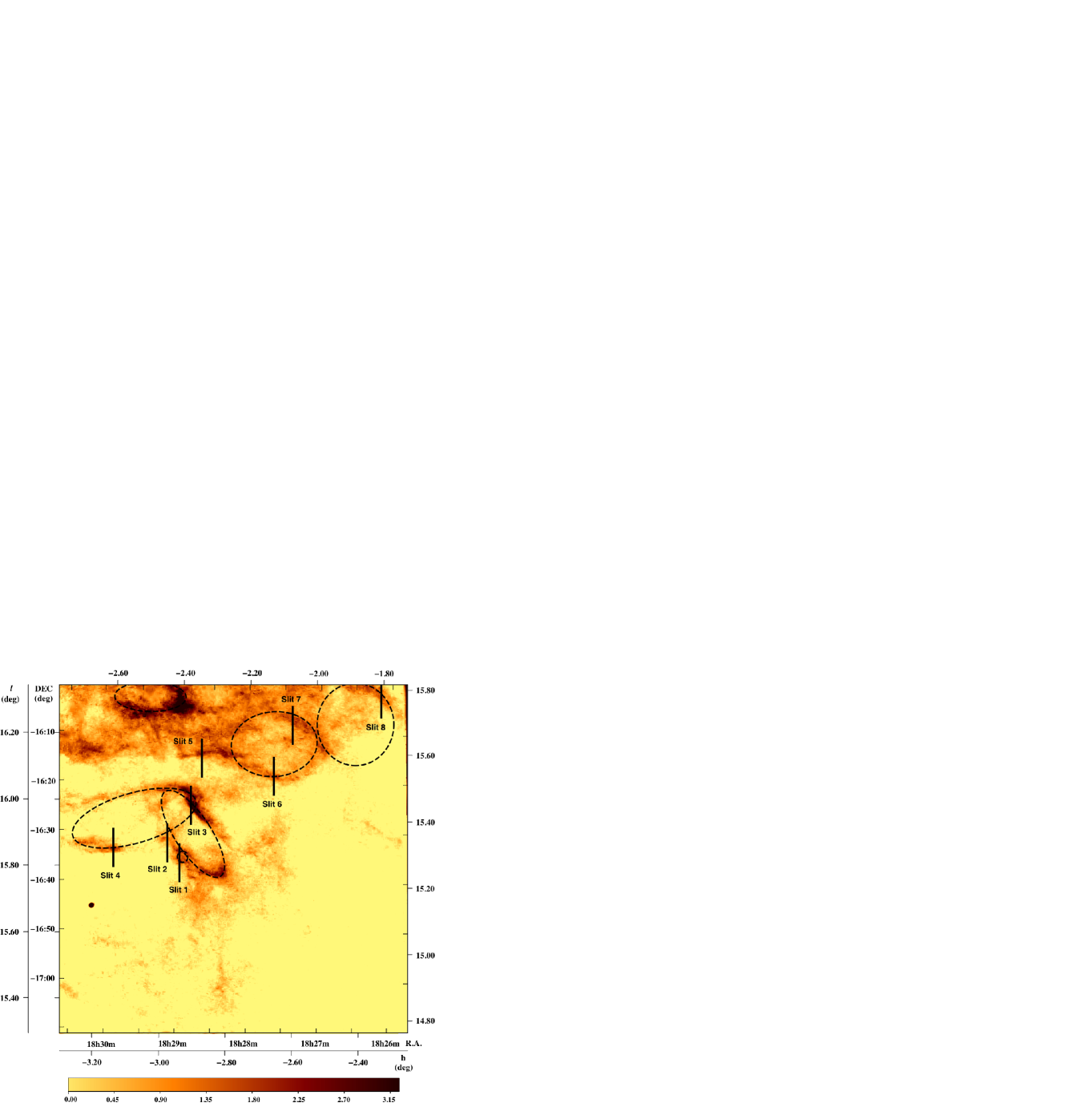
Figure 1: The continuum–subtracted image of the observed area in Sagittarius, in H$\alpha+[$N ii$]$ emission in both equatorial (R.A., Dec internal lines on axis) and galactic (l, b external lines on axis) coordinates. The black lines indicate the positions of the slits and the dashed-ellipses the geometry of the newly discovered candidate SNRs. Shadings run linearly from 0 to 3.2$\times$$10^{-17}$ erg s^-1 cm^-2 arcsec^-2.

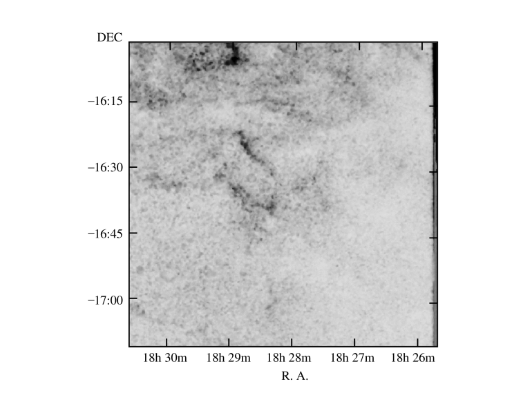
Figure 2: The continuum–subtracted image of the observed area in $[$S ii$]$ emission. Shadings run linearly from 0 to 90$\times$$10^{-17}$ erg s^-1 cm^-2 arcsec^-2.

All images were taken with the 0.3 m Schmidt–Cassegrain (f/3.2) telescope at Skinakas Observatory in Crete, Greece, in 2005 June 7, 8 and 9, and August 26 and 28. A 1024 $\times$ 1024 Thomson CCD was used which has a pixel size of 19 $\mu$m resulting in a 70′ $\times$ 70′ field of view and an image scale of 4″ pixel^-1. The area of interest was observed for 2400 s in H$\alpha+[$N ii$]$, $[$S ii$]$ and $[$O iii$]$ filters, while corresponding continuum images were also observed (180 s each) and after the appropriate scaling were subtracted from the narrow-band images to eliminate the confusing star field. The continuum subtracted images of the H$\alpha+[$N ii$]$ and $[$S ii$]$ emission lines are shown in Figs. 1 and 2.

The image reduction was carried out using the IRAF and MIDAS packages. All frames were bias subtracted and flat–field corrected using a series of twilight flat–fields. The absolute flux calibration was performed through observations of a series of spectrophotometric standard stars (HR5501, HR7596, HR7950, HR8634 and HR9087; Hamuy et al. 1992). The astrometric solution for all data frames was calculated using the Space Telescope Science Institute (STScI) Guide Star Catalogue II (GSC–II; Lasker et al. 2008). All the equatorial coordinates quoted in this work, refer to epoch 2000.

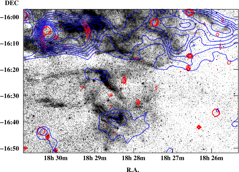
Figure 5: The correlation between the SuperCOSMOS H$\alpha$ mosaic image and the radio emission from archival data at 4850 MHz (blue line) and 1400 MHz (red line). The blue contours scale linearly from 2.0$\times 10^{-2}$ Jy/beam to 0.2 Jy/beam, with step 0.02 Jy/beam and the red from 1.2$\times 10^{-3}$ Jy/beam to 4.0$\times 10^{-3}$ Jy/beam, with step 9.3$\times 10^{-4}$ Jy/beam.

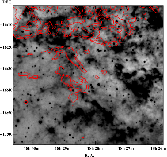
Figure 6: The correlation between the infrared WISE emission at 22$\mu$m image and the H$\alpha+[$N ii$]$  emission (red lines). The red contours values are 70 (low) and 130 (high) $\times$$10^{-17}$ erg s^-1 cm^-2 arcsec^-2.

In order to cover in full the area of interest, we used wide–field images from the SuperCOSMOS H$\alpha$ Survey (SHS; Parker et al. 2005). The resulting 1.4°$\times$ 1.0° mosaic was created from 16 different fields, each one having a 30′ $\times$ 30′ field of view and an image scale of 0.67″ pixel^-1. The mosaic was used in order to compare the detected optical emission with other wavebands (radio and infrared – see Sect. 3.3 and Figs. 5, 6). The details of all imaging observations are given in Table 1.

2.2 Spectroscopy

Low dispersion long–slit spectra were obtained with the 1.3 m Ritchey–Cretien (f/7.7) telescope at Skinakas Observatory in 2005 June 4 and 5, July 10 and September 6 and 7. The 1300 line mm ^-1  grating was used together with a 2000 $\times$ 800 SITe CCD (15 $\times$ 15 $\mu$m² pixels) resulting in a scale of 1Å pixel^-1 and covering the range 4750 Å – 6815 Å. The above combination results in a spectral resolution of $\sim$8 and $\sim$11 Å in the red and blue wavelengths, respectively. The slit width was 7$\aas@@fstack{\prime\prime}$7 and its length 7$\aas@@fstack{\prime}$9 and in all cases was oriented in the south–north direction. The spectrophotometric standard stars HR4468, HR5501, HR7596, HR9087, HR8634, and HR7950 (Hamuy et al., 1992) were observed to calibrate the spectra. The data reduction was performed using the IRAF package (twodspec).

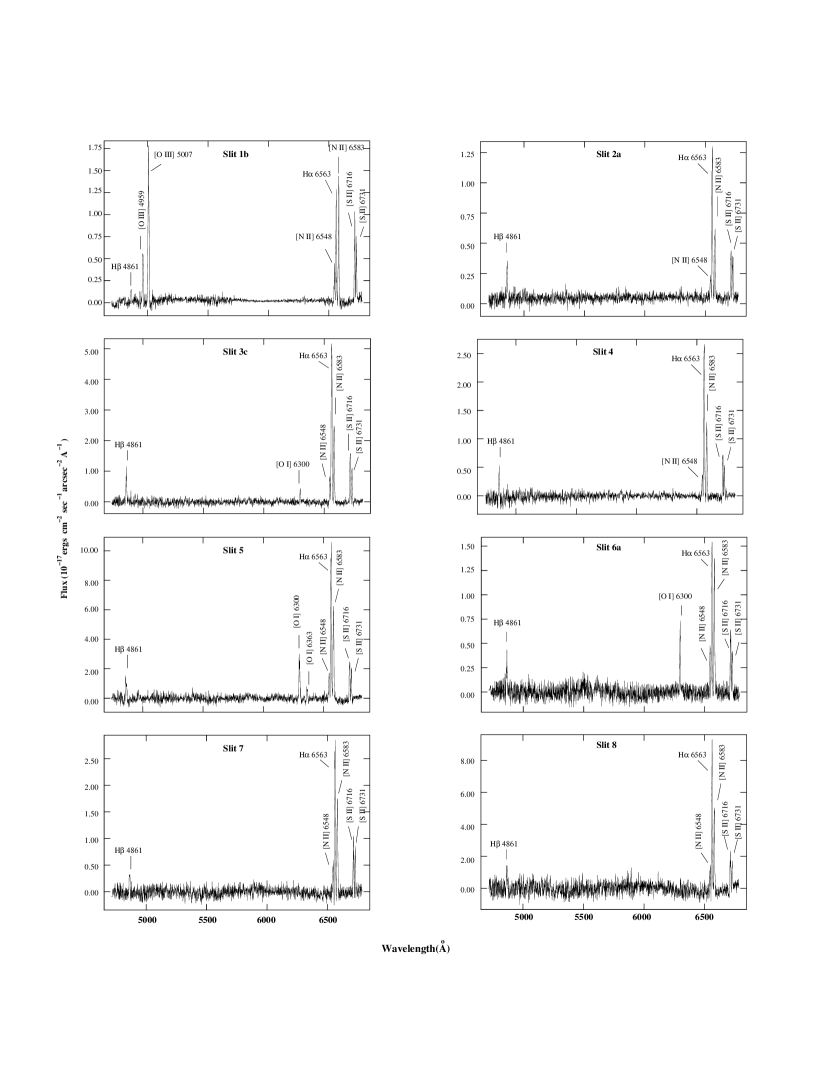
Figure 3: Long–slit spectra from different positions of the observed area (see Table 1).

The deep low resolution spectra were taken on the relatively bright optical filament (their exact positions are given in Table 1). In Table 5, we present the relative line fluxes taken from different apertures (a, b and c) along each slit. In particular, apertures a, b and c have an offset (see Table 1) north or south of the slit center which were selected because they are free of field stars in an otherwise crowded field and they include sufficient line emission to permit an accurate determination of the observed line fluxes (their exact aperture length is given in Table 1). The background extraction aperture was taken towards the northern end or the southern end of the slits depending on the slit position. The signal to noise ratios presented in Table 5 do not include calibration errors, which are less than 10 percent. Typical spectra are shown in Fig. 3.

3 Results

3.1 The optical emission line images

The images in Figs. 1 and 2 show considerable new faint optical emission including filamentary and diffuse structures. The H$\alpha+[$N ii$]$ (Fig. 1) best describes the newly detected structures, while the $[$S ii$]$ image (Fig. 2) also shows strong emission but less filamentary structure. In contrast, $[$O iii$]$ emission was only detected in one small area and it is not shown here.

All images being flux calibrated provide a first indication of the nature of the observed emission (see Table 2). A study of these images shows that most parts of the optical emission originate from shock heated gas since we estimate ratios $[$S ii$]$/H$\alpha$$\geq$0.47. This conclusion is verified by the deep long–slit spectra which offer more accurate measurements of the individual line fluxes. The variety of structures detected in the H$\alpha+[$N ii$]$ and $[$S ii$]$ images are not present in the medium ionization line of $[$O iii$]$ apart from one area (Slit 1), hence the 3$\sigma$ upper limit, over the area is given in Table 2.

Several thin and curved filaments can be seen in Fig. 1. In general, the field appears somewhat complex due to the presence of many filamentary structures and significant number of diffuse emission structures. A search in the database did not reveal any known bright optical nebula. A combination of their morphology and the spectroscopic results suggest the existence of more than one possible SNR in the region. In particular, following their geometry we suggest the existence of six candidate SNRs (indicated as dashed-ellipses in Fig. 1). Their names, centers and diameters are presented in Table 3. Of course, the possibility of less or more SNRs in the region cannot be ruled out.

The most interesting filaments of the candidate SNRs are described here in more detail.

G 15.6$-$2.6. The basic characteristic of its filaments is their brightness in H$\alpha+[$N ii$]$ (Fig. 1) and $[$S ii$]$ (Fig. 2). The bulk of the emission seems to be bounded by at least two very bright complex filaments. The southern structure covers the area from $\delta$$\sim-$16°39′, $\alpha$$\simeq$18^h28^m21^s to $\delta$$\sim-$16°33′, $\alpha$$\simeq$18^h29^m01^s, while the northern, having the same inclination ($\sim$45°), with respect to the east–west direction, covers the area between $\delta$$\sim-$16°29′, $\alpha$$\simeq$18^h28^m31^s and $\delta$$\sim-$16°21′, $\alpha$$\simeq$18^h28^m55^s. No significant emission was found in the image of the $[$O iii$]$ medium ionization line. The morphology of the $[$S ii$]$ image is generally similar to, though not as bright as, that of the H$\alpha+[$N ii$]$ image. We detected $[$S ii$]$ emission where most of the H$\alpha+[$N ii$]$ emission was found with filamentary bright structures in the south–east and north–west areas, while diffuse emission characterizes the rest of the remnant’s emission. Diffuse emission and several shorter filamentary structures are detected between the north and south boundaries. The images show $[$S ii$]$/H$\alpha$$\geq$0.7 in agreement with the two spectra positions (slits 1 & 3) which show $[$S ii$]$/H$\alpha$$\geq$1.0. It should be noted that part of the filaments in the south and to the north seem to correlate with the radio and infrared emission but their resolution does not permit to verify or not such a correlation (see Section 3.3). New pointed radio observations are needed to come into secure conclusion.

G 15.8$-$2.8. The most interesting regions lie in the south–east and north–west, where bright filamentary structures are present (between $\alpha$$\simeq$18^h29^m45^s, $\delta$$\simeq$–16°34′20″; $\alpha$$\simeq$18^h30^m26^s, $\delta$$\simeq$–16°32′17″ and $\alpha$$\simeq$18^h28^m48^s, $\delta$$\simeq$–16°22′45″; $\alpha$$\simeq$18^h28^m58^s, $\delta$$\simeq$–16°21′15″). There are also fainter filaments and diffuse emission which cover most of the suggested SNR area, both to the north (from the bright north–west filament to $\alpha$$\simeq$18^h30^m33^s, $\delta$$\simeq$–16°25′00″) and south (from the bright south–east filament to $\alpha$$\simeq$18^h28^m47^s, $\delta$$\simeq$–16°25′30″). Similarly to the previous candidate SNR, no $[$O iii$]$ emission was detected. Both images and spectra (slits 2 & 4) show similar $[$S ii$]$/H$\alpha$ (between 0.47 and 0.60). Part of this SNR to the west overlaps with the north filament of the previous SNR, however their morphology and curvature suggest that the filamentary structures are separated and they probably do not correlate with each other. Also, there is a gap of $\sim$1′ between the very bright filaments and they both show infrared emission, while it seems that only the filament from this candidate SNR correlates with the radio emission (Section 3.3). However, due to the low resolution of the radio observations, the possibility that the radio emission comes from both SNRs cannot be ruled out. It should be noted that because the radio emission is generally weak, the overlap of the two remannts would certaintly make it brighter. Also, the fact that the high frequency radio emission correlates better with the optical than the low frequency, which might suggests a flatter radio spectrum and therefore thermal radio emission, should be examined further by new pointed radio observations in order to verify their nature.

G 15.8$-$2.2. The faint filamentary and diffuse emission of this candidate SNR forms a well defined ellipse (Fig. 1). There is a bright structure to the east ($\alpha$$\simeq$18^h28^m20^s, $\delta$$\simeq$–16°14′25″) and many small filaments all around the SNR’s borders. The $[$S ii$]$/H$\alpha$ emission suggests shock–heated mechanisms ($\sim 0.6$) in agreement with that from the spectra (slits 6 & 7) which is between 0.45 and 0.7. There is also a bright filament further to the east (from $\alpha$$\simeq$18^h28^m28^s, $\delta$$\simeq$–16°14′00″ to $\alpha$$\simeq$18^h28^m56^s, $\delta$$\simeq$–16°15′05″) with shock–heated emission, having however the weakest $[$S ii$]$  measured in the area ($[$S ii$]$/ha$=$0.45; slit 5). Following its morphology, it is probable that it is not related to this remnant, however, their correlation cannot be ruled out completely. There is also radio and infrared emission which might correlates with the optical in some of the SNR’s regions (Section 3.3), while $[$O iii$]$ emission has not been detected.

G 15.8$-$1.9. In contrast to the previous SNR candidates, this is the fainter one in both H$\alpha+[$N ii$]$ and $[$S ii$]$ images, having less filamentary and more diffuse emission, while $[$O iii$]$ was not detected. Its brightest part is to the north–northwest (from $\alpha$$\simeq$18^h26^m00^s, $\delta$$\simeq$–16°04′25″ to $\alpha$$\simeq$18^h26^m40^s, $\delta$$\simeq$–16°00′20″), there is fainter emission to the east ($\alpha$$\simeq$18^h26^m50^s, $\delta$$\simeq$–16°13′45″), while no emission has been detected to the south. The $[$S ii$]$/H$\alpha$ ratios of 0.48 (spectrum, slit 8) and 0.50 (imaging) suggest that a shock–heated mechanism produced the emission while the optical emission correlates well with the radio and partially with the infrared (Section 3.3).

G 16.2$-$2.5. This is the brightest candidate in H$\alpha+[$N ii$]$ and $[$S ii$]$ with $[$S ii$]$/H$\alpha$$\sim 0.5$. There are bright thick filaments almost all around the remnant (south from $\alpha\simeq$ 18^h28^m45^s, $\delta\simeq$ –16°06′10″ to $\alpha\simeq$ 18^h29^m55^s, $\delta\simeq$ –16°03′30″; west from $\alpha\simeq$ 18^h28^m45^s, $\delta\simeq$ –16°06′40″ to $\alpha\simeq$ 18^h28^m56^s, $\delta\simeq$ –16°01′30″ and north–west to $\alpha\simeq$ 18^h29^m14^s, $\delta\simeq$ –15°59′45″) with a width of $\sim$2–3′(due to the position of this candidate SNR, the north part can only be seen in Fig. 5). Weaker and diffuse emission patches are located in its north–east area while no $[$O iii$]$ emission was found. The detected emission line structures are also bounded in all directions by diffuse emission which is probably due to H ii regions. It is very close to the only known radio SNR G 16.2–2.7 but their position and morphology suggest that they are not related to each other (see Fig. 5). However, a small possibility that this emission is related to the radio remnant still remains if we consider that they can be seen by a different angle to the line of sight. Kinematic oobservations could confirm or reject the latter scenario. There is also infrared emission in the area which partially correlates with the optical (Section 3.3).

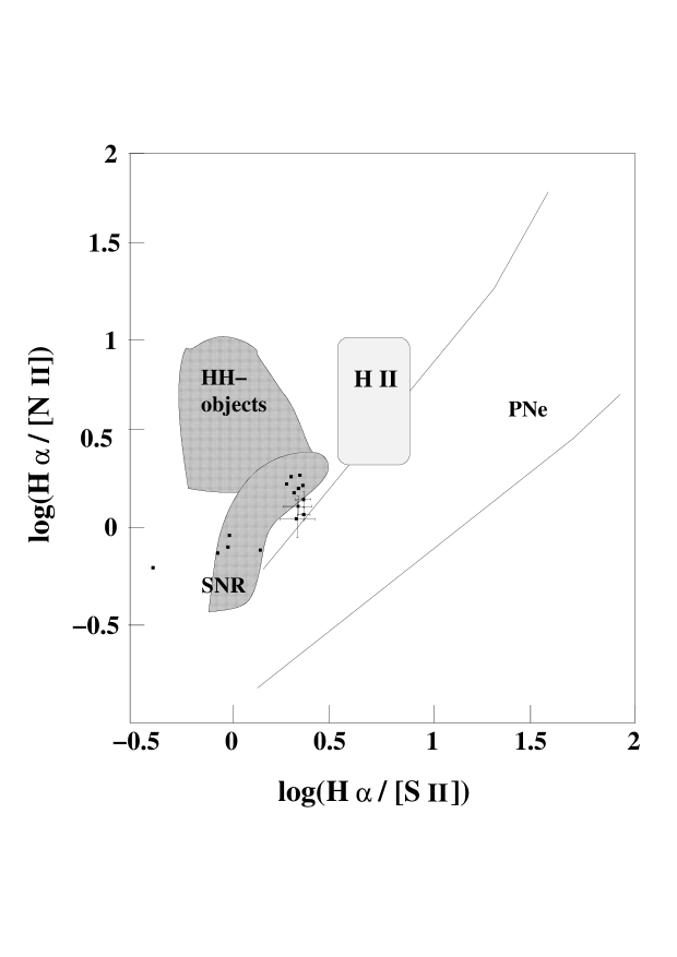
Figure 4: Diagnostic diagram (Sabbadin et al. (1977); Cantó (1981)), where the positions of line ratios listed in Table 1, from Slit 1a to 8, are shown in black squares. For those which are not within the SNR region the calculated errors have taken into account.

G 15.6$-$2.7. This is the most peculiar region since it is the only area that shows strong $[$O iii$]$ and very strong $[$N ii$]$ emission. A shock–heated mechanism is responsible for the emission found since the $[$S ii$]$/H$\alpha$$>$1.0. Its morphology, size and position in the diagnostic diagram (Fig. 4) let us conclude that it should be a SNR which might not related to G 15.6$-$2.6, however their correlation cannot be ruled out so further investigation (i.e. high resolution spectroscopic observations) is needed in order to identify its origin. In case they are related, then the possibility that its $[$S ii$]$ emission is background emission from G 15.6$-$2.6 and it does not come from this object will change the responsible mechanism to photoionization and then it might not be an SNR but a planetary nebula. Note that the strong $[$O iii$]$ emission is not unusual to be found in both SNRs and PNe so it cannot be used as a distiguishable criterion. In Table 2 a typical $[$O iii$]$ flux is given. Radio emission is not found to be correlated with this SNR candidate while there is faint infrared emission in its vicinity which might associate with it. (Section 3.3).

3.2 The optical spectra

Deep long–slit spectra were taken in order to accurately determine the nature of the observed emission by measuring the strengths of the H$\alpha$ and $[$S ii$]$ emission lines. Eight different spectra, extracted from the relatively brightest optical filaments, are shown in Fig. 3 and the measured fluxes are given in Table 5. Different apertures (a, b and c) were extracted from each spectrum along the slit which have an offset (see Table 1) north or south of the slit center. The selection criteria were to be in an area which is free of field stars and they include sufficient line emission to permit an accurate determination of the observed line fluxes. The background extraction aperture was taken towards the northern end or the southern end of the slits depending on the slit position. The signal to noise ratios presented in Table 5 do not include calibration errors, which are less than 10 percent.

The properties of the spectra strongly point to emission from shock heated gas ($[$S ii$]$/H$\alpha$ ratios between 0.44 to 1.20, $[$N ii$]$/H$\alpha$ ratios between 0.53 to 1.35; presence of $[$O i$]$ emission; Table 5). The filamentary nature of the newly discovered optical radiation, as seen in the narrow band images, also supports this conclusion. The absolute H$\alpha$ flux covers a range of values from 0.6 to 41.3 $\times$ $10^{-17}$ erg s^-1 cm^-2 arcsec^-2. The $[$S ii$]\lambda\lambda\ 6716/6731$ ratio that was measured between 1.2 and 1.5, indicates low electron densities (below 240 cm^-3; Osterbrock & Ferland 2006 and below 400 cm^-3 by taking into account the statistical errors on the sulfur lines; Shaw & Dufour 1995).

Although, the low ionization lines are quite strong, $[$O iii$]$ line emission at 5007 Å is only detected at pos. 1 (Table 2), suggesting shock velocities $\sim$120 km s^-1 (cox85) and below 200 km s^-1 (Allen et al., 2008) in that area. Also, the $[$O iii$]$/H$\beta$ is $>$ 6, according to theoretical models (Raymond et al., 1988), suggest the presence of shocks with incomplete recombination zones. The relatively weak H$\beta$ emission and the absence of $[$O iii$]$ emission in all the other positions suggest significant interstellar attenuation of the optical emission and they could be explained by slow shocks propagating into the interstellar clouds ($\leq$ 100 km s^-1; Hartigan et al. 1987).

The log(H$\alpha$/$[$N ii$]$) versus log(H$\alpha$/$[$S ii$]$) intensities, from Table 5, corrected for interstellar extinction, are compared with others of well defined phenomena in Fig. 4 (following Sabbadin et al. 1977 & Cantó 1981) and show that all positions are within or very close to (taking into account the calculated error for those which are not within) the area designated for SNRs.

3.3 Observations at other wavelengths

Radio emission in the area of the optical structures is detected in the low resolution (7′) 4850 MHz images of the Green Bank survey (Condon et al., 1991). In most of the cases, the radio emission matches with the optical emission but given the low resolution, it is hard to make a detailed spatial correlation apart from confirming their association. We have also examined the higher resolution CGPS data at 1420 MHz (Taylor et al., 2003) but no prominent emission was detected to be correlated with the optical. The observed filaments are located close to radio contours (Fig. 5), in many cases there is a good correlation but the low resolution of the radio images does not allow us to determine the relative position of the filament with respect to the shock front. Higher resolution radio observations in different wavelengths should be performed to provide conclusive evidence on the nature of the sources as SNRs.

We have also searched ROSAT All–sky survey data for X–ray emission but it is very faint and diffuse and we can not identify the sources in detail. We also searched the VLA Galactic Plane Survey (VGPS; Stil et al. 2006) for Hi kinematics data but unfortunately the area of interest is not covered by this survey.

In order to explore how the optical emission correlates with the infrared, we searched all the available data at NASA/IPAC Infrared Science Archive. In particular, we examined the GLIMPSE/Spitzer (Churchwell et al., 2009), the WISE (Wright et al., 2010) and the IRIS (Miville–Desch$\hat{\rm e}$nes & Lagache, 2005) images of the same area. Unfortunately, the area we are interested in was not covered by the GLIMPSE survey at 3.6, 4.5, 5.8 and 8.0 $\mu$m (resolution at 1.2″) while the IRIS at 25, 60 and 100 $\mu$m (resolution from 30″ to 2′) data revealed clear enhancement of infrared emission in the area where the optical emission of the candidate SNRs is detected, however the low-resolution maps do not permit a detailed comparison. On the other hand, the WISE data at 3.4, 4.6, 12 and 22 $\mu$m (resolution of 6.1, 6.4, 6.5 and 12″, respectively) show evidence of correlation with the optical and/or radio emission in the last two channels. In particular, both the 12 and 22 $\mu$m show evidence of association with the optical and radio filamentary structures of the candidate SNRs. Since the 12 $\mu$m image has essentially the same features with the 22 $\mu$m but they appear to be stronger in the latter, in Fig. 6 we present a greyscale representation of the 22 $\mu$m image with overlapping contours of the optical emission. In a few cases, the infrared emission seems to follow the morphology of the candidate SNRs suggesting their possible association which is expected since it is known that the shocked gas cools through emission lines, and many important emission lines occur in the mid–infrared. A similar case is that of the SNR G 296.7$-$0.9 (Robbins et al., 2012) where possible association of this SNR with the infrared emission was found. It should also be noted that the appearance of the infrred emission in the vicinity and not on the optical emission in most of the cases is expected, since in general there is not a very good correlation between the infrared and the H$\alpha$ emission (Reach et al., 2006).

4 Discussion

The newly discovered candidate SNRs towards the Sagittarius constellation show up as incomplete circular or elliptical structures in the optical and in most of the cases in the radio and without any X–ray and H i emission detected so far. The absence of soft X–ray emission may indicate a low shock temperature and/or a low density of the local interstellar medium. Its optical emission marginally correlates with the infrared. The elliptical shape of the candidate SNRs is unusual compared to most known SNRs suggesting that the surrounding medium is very irregular with not constant interstellar density. However, it should be mentioned that a significant number of known SNRs show not circular structure (bilateral, barriel, elliptical, cilindrical etc.) depending on their position to the line of sight so this might also be a reason of their appearance.

Detailed optical observations have been performed in an attempt to understand the nature of the candidate SNRs. The lower ionization images in H$\alpha+[$N ii$]$ and $[$S ii$]$ reveal several filamentary and diffuse structures while the higher ionization image in $[$O iii$]$  shows emission only in one region. The H$\alpha+[$N ii$]$ image best describes the newly detected structures. Sulfur line emission is also detected and generally appears less filamentary and more diffuse than in the H$\alpha+[$N ii$]$ image with their position and shape in agreement with that of the H$\alpha+[$N ii$]$. The $[$O iii$]$ flux production depends mainly on the shock velocity and the ionization state of the preshocked gas. Therefore, as mentioned in Sect. 3.1, the absence of $[$O iii$]$ emission in almost all of the areas may be explained by slow shocks propagating into the ISM. The presence of [O i] 6300 Å line emission is also consistent with the emission being from shocked material. The $[$O iii$]$/H$\beta$ ratio is a very useful diagnostic tool for complete or incomplete shock structures (Raymond et al., 1988). However, the absence of $[$O iii$]$ does not allow us to suggest for complete or incomplete shock structures apart from pos.1 where shocks with incomplete recombination zones should be present. Both the calibrated images and the long–slit spectra suggest that the detected emission results from shock heated gas since the $[$S ii$]$/H$\alpha$ ratio exceeds the empirical SNR criterion value of 0.4–0.5, while the measured $[$N ii$]$/H$\alpha$ ratio also confirms this result.

The SNR origin of the proposed candidate remnants is strongly suggested by the positions of the line ratios in Fig. 4 compared with those of Herbig–Haro objects, Hii regions and planetary nebulae (PNe). They follow closely the shape of those observed for those of shock ionized evolved SNRs.

The H$\alpha$/H$\beta$ ratios in Table 5 can be used to estimate the variations in logarithmic extinction coefficient c over these sources, assuming an intrinsic ratio of 3 and the interstellar extinction curve as implemented in the nebular package (Shaw & Dufour, 1995) within the IRAF software. An interstellar extinction c (see Table 5) between 0.2 and 1.1 or an A_V between 0.4 and 2.2 were measured, respectively. We have also determined the electron density measuring the density–sensitive line ratio of $[$S ii$]\lambda\lambda\ 6716/6731$. The measured densities lie below 240 cm^-3.

The candidate remnants under investigation have not been studied in the past hence the current stage of their evolution is unknown. Our aim is to provide a first indication of their stage of evolution by estimating basic SNR parameters, assuming that the temperature is close to 10⁴ K.

Estimated values of N_H between 4.8 and 6.8 $\times 10^{21}$ cm^-2 and N_H between 3.2 and 7.4 $\times 10^{21}$ cm^-2 are given by Dickey & Lockman (1990) and Kalberla et al. (2005) respectively, for the column density in the direction of the candidate remnants. Using the relations of Ryter et al. (1975) and Predehl & Schmitt (1995), we obtain N_H between 0.9 and 4.9 $\times 10^{21}\leavevmode\nobreak\ {\rm cm}^{-2}$ for the minimum and maximum c values calculated from our spectra. In Table 3, we present the estimated values of N_H for each candidate remnant, where it can be seen that the values based on the optical data and the statistical relations are consistent with the estimated galactic N_H  from Kalberla et al. (2005) and less by that estimated from Dickey & Lockman (1990). However, it should be noted that the slightly higher values calculated by the latter method can be explained by the fact that it also covers gas beyond the area of interest. Assuming that they are still in the adiabatic phase of their evolution the preshock cloud density n_c can be measured by using the relationship (Dopita, 1979)

$${\rm n_{[SII]}\simeq\ 45\ n_{c}V_{\rm s}^{2}}\leavevmode\nobreak\ {\rm cm^{-3}},$$ (1)

where ${\rm n_{[SII]}}$ is the electron density derived from the sulfur line ratio and V_s is the shock velocity into the clouds in units of 100 km s^-1. Furthermore, the blast wave energy can be expressed in terms of the cloud parameters by using the equation given by McKee & Cowie (1975)

$${\rm E_{51}}=2\times 10^{-5}\beta^{-1}{\rm n_{c}}\ V_{\rm s}^{2}\ {\rm r_{s}}^{3}\ \ {\rm erg}.$$ (2)

The factor $\beta$ is approximately equal to 1 at the blast wave shock, ${\rm E_{51}}$ is the explosion energy in units of 10⁵¹ erg and r_s the radius of the remnant in pc.

By using the upper limit on the electron density of 240 cm^-3, which was derived from our spectra, we obtain from Eq. (1) that ${\rm n_{c}}V_{\rm s}^{2}<5.3$. Then Eq. (2) becomes ${\rm E_{51}}<\alpha\times 10^{-3}\leavevmode\nobreak\ {\rm D_{1kpc}^{3}}$, where $\alpha$ is a value depends on the diameter of each candidate remnant and ${\rm D_{1kpc}}$ the distance to the remnant in units of 1 kpc. For the different diameters of the remnants and assuming the typical value of 1 for the supernova explosion energy (E₅₁), we derive that the candidate SNRs lie at distances greater than 8 kpc. Since, there are no other measurements of the interstellar density n₀, values of 0.1 and 1.0 will be examined. Then, the lower interstellar density of $\sim$0.1 cm^-3 suggests that their distance is between 10 and 22 kpc while for n${}_{0}\approx 1\leavevmode\nobreak\ {\rm cm}^{-3}$ it is between 1.0 and 2.2 kpc, for the lower and higher column densities calculated above. Combining the previous results, values between 0.1 and 0.2 cm^-3 for the interstellar density seem to be more probable. It should also be noted that the ambient density of gas around the candidate SNRs is not the same so this might also change the estimated vaues.

We also searched for pulsars in the region using the ATNF Pulsar Catalogue (Manchester et al., 2005). In total, we found 8 pulsars within a 1.5$\degr$ diameter circle away from the center of each candidate SNR. In Table 5, we present their names, coordinates and rotation period as well as which candidate SNRs fulfill the 1.5$\degr$ limit. The closest one is PSR1826-1526 to G 15.8$-$1.9 at a distance of 0.7$\degr$. It is not clear at the moment if any of these pulsars are related to the candidate SNRs, however, the existence of a significant number of pulsars very close to the area of the candidate SNRs it is another strong indication of the existence of more than one SNRs in the region. It is more plausible that due to their distance from the candidate SNRs they are not associated with them since the closest pulsar is about 4 radii from the nearest SNR or $>$ 75 pc in the plane of the sky at a distance of 8 kpc. However, if they are not in the plane of the sky which is probably the case, then these numbers might change. Also, they might be at different distances which change the numbers, too. Therefore, their correlation cannot be confirmed or ruled out and it should be further examined in the future in detail.

It is possible that this irregular group of filaments is part of a wider structure but is being seen through holes in intervening clouds, leading to patchy optical interstellar extinction. The current data are not sufficient to claim strong a correlation. Furthermore, there is a possibility that the detected optical emission could be part of a number of supernova explosions in the area. However, since neither the distance nor the interstellar medium density are accurately known, we cannot confidently determine the current stage of evolution of the candidate remnants and more observations are needed.

Further study of the area would benefit from higher resolution multiwavelength observations (optical, radio and X–ray) and will help to clarify the current uncertainties. In particular, higher resolution imaging observations will verify their filamentary structure and confirm their morphological appearance, while kinematic observations will help to determine their 3-D morphology and measure expansion velocities. X–ray observations will help in order to clarify if there is any correlation of the faint and diffuse X–ray emission with the optical filaments and provide more information about their evolutionary stage, while radio observations would also be useful to examine their non–thermal spectral index and confirm their SNR nature.

Table 1: Imaging and Spectral log

IMAGING
Filter	$\lambda_{\rm c}$	$\Delta\lambda$	Total exp. time	telescope
	(Å)	(Å)	(sec)
H$\alpha+$[N ii] 6548 & 6584 Å	6570	75	4800 (2)	0.3m Skinakas
$[$O iii$]$ 5007 Å	5005	28	4800 (2)	0.3m Skinakas
$[$S ii$]$ 6716 & 6731 Å	6720	18	4800 (2)	0.3m Skinakas
Cont blue	5470	230	180	0.3m Skinakas
Cont red	6096	134	180	0.3m Skinakas
H$\alpha+$[N ii] 6548 & 6584 Å		80	10800	1.2m AAO/UKST
SPECTROSCOPY
Slit position	Slit centers		Offset	Aperture length
	$\alpha$	$\delta$
	(h m s)	(° ′ ″)	(arcsec)	(arcsec)
1a	18 29 09	$-$16 31 32	2.4 N	10.6
1b	18 29 09	$-$16 31 32	28.9 S	18.9
2a	18 28 58	$-$16 36 00	95.0 N	26.0
2b	18 28 58	$-$16 36 00	70.2 N	11.8
2c	18 28 58	$-$16 36 00	19.5 N	13.0
3a	18 28 49	$-$16 24 55	137.5 N	27.1
3b	18 28 49	$-$16 24 55	33.6 N	43.6
3c	18 28 49	$-$16 24 55	20.1 S	23.6
4	18 29 55	$-$16 34 12	16.6 S	30.7
5	18 28 42	$-$16 15 02	37.2 S	60.2
6a	18 27 41	$-$16 17 39	74.3 S	30.7
6b	18 27 41	$-$16 17 39	116.2 S	20.0
7	18 27 26	$-$16 07 50	32.4 N	31.9
8	18 26 12	$-$16 01 58	27.7 N	23.6

Table 2: Typically fluxes measured over the brightest filaments.

	Slit 1	Slit 2	Slit 3	Slit 4	Slit 5	Slit 6	Slit 7	Slit 8
H$\alpha+[$N ii$]$	42.8	62.8	114.3	64.1	67.2	50.4	57.9	53.8
$[$S ii$]$	19.5	18.8	40.0	16.6	15.8	15.6	17.1	13.5
$[$O iii$]$	236	$<$45
$[$S ii$]$/H$\alpha$	0.91	0.60	0.70	0.52	0.47	0.62	0.59	0.50

Table 3: New candidate SNRs.

SNR name	SNR center		Diameter	NH		NH
	$\alpha$	$\delta$		Kal	D&L	Ral & P&S
	(h m s)	(° ′ ″)	(arcmin)	($\times 10^{21}$ cm-2)	($\times 10^{21}$ cm-2)	($\times 10^{21}$ cm-2)
G 15.6$-$2.6	18 28 46.1	$-$16 30 40	3.7$\times$10.2	4.6	6.8	1.0–4.9
G 15.8$-$2.8	18 29 35.8	$-$16 27 40	5.1$\times$12.9	3.2	4.8	1.0-4.9
G 15.8$-$2.2	18 27 38.8	$-$16 12 17	6.5$\times$8.7	4.6	6.8	2.6–3.3
G 15.8$-$1.9	18 26 30.7	$-$16 08 00	7.7$\times$8.3	7.4	6.8	0.7–4.8
G 16.2$-$2.5	18 29 23.5	$-$16 03 06	3.0$\times$7.2	4.6	6.2	2.8–3.5
G 15.6$-$2.7	18 28 53.5	$-$16 35 34	1.1$\times$1.1	4.6	6.8	2.0-4.8

Table 4: Relative line fluxes.

	Slit 1a			Slit 1b			Slit 2a			Slit 2b			Slit 2c
Line (Å)	F	I	S/N	F	I	S/N	F	I	S/N	F	I	S/N	F	I	S/N
H$\beta$ 4861	23	35	13	15	35	2	19	35	27	21	35	18	24	35	21
[O iii] 4959	13	20	7	66	147	5	$-$	$-$	$-$	$-$	$-$	$-$	$-$	$-$	$-$
[O iii] 5007	36	53	23	187	405	13	$-$	$-$	$-$	$-$	$-$	$-$	$-$	$-$	$-$
$[$O i$]$ 6300	14	14	17	$-$	$-$	$-$	$-$	$-$	$-$	$-$	$-$	$-$	$-$	$-$	$-$
[N ii] 6548	32	32	36	36	36	5	14	14	42	15	15	22	13	12	42
H$\alpha$ 6563	100	100	89	100	100	14	100	100	216	100	100	123	100	100	137
[N ii] 6584	95	95	82	100	99	14	40	39	103	44	43	58	42	42	66
[S ii] 6716	63	61	59	74	69	10	27	26	71	31	29	44	30	29	44
[S ii] 6731	49	47	47	53	49	7	22	21	56	26	25	38	26	23	38
Absolute H$\alpha$ flux	7.5			0.62			16.7			13.3			11.9
[S ii]/H$\alpha$	1.08 $\pm$ 0.02			1.20$\pm$ 0.1			0.47$\pm$ 0.03			0.54 $\pm$0.05			0.51$\pm$ 0.04
F(6716)/F(6731)	1.30 $\pm$ 0.04			1.4$\pm$ 0.3			1.3$\pm$ 0.1			1.2$\pm$ 0.1			1.3$\pm$ 0.1
[N ii]/H$\alpha$	1.28$\pm$ 0.02			1.35$\pm$ 0.1			0.53$\pm$0.03			0.58$\pm$ 0.06			0.54$\pm$ 0.05
c(H$\beta$)	0.52$\pm$ 0.10			1.1$\pm$ 0.6			0.74$\pm$ 0.05			0.64$\pm$ 0.07			0.50$\pm$ 0.06
EB-V	0.37 $\pm$ 0.07			0.7 $\pm$ 0.4			0.51 $\pm$ 0.03			0.44 $\pm$ 0.05			0.34 $\pm$ 0.04
	Slit 3a			Slit 3b			Slit 3c			Slit 4			Slit 5
Line (Å)	F	I	S/N	F	I	S/N	F	I	S/N	F	I	S/N	F	I	S/N
H$\beta$ 4861	15	35	18	20	35	44	18	35	32	28	35	16	20	35	21
$[$O i$]$ 6300	9	10	26	5	5	33	7	7	31	$-$	$-$	$-$	24	25	61
$[$O i$]$ 6363	$-$	$-$	$-$	$-$	$-$	$-$	$-$	$-$	$-$	$-$	$-$	$-$	12	12	27
[N ii] 6548	17	16	38	16	16	85	18	18	66	15	14	21	15	15	37
H$\alpha$ 6563	100	100	165	100	100	337	100	100	243	100	100	115	100	100	194
[N ii] 6584	96	95	73	44	44	180	49	48	141	47	47	58	57	56	122
[S ii] 6716	63	60	28	28	26	115	31	29	94	27	26	36	27	26	57
[S ii] 6731	49	45	16	20	18	88	21	19	70	21	20	28	20	19	42
Absolute H$\alpha$ flux	14.1			27.0			26.3			10.7			20.2
[S ii]/H$\alpha$	1.05$\pm$ 0.09			0.45 $\pm$0.02			0.49 $\pm$ 0.03			0.47$\pm$ 0.05			0.45 $\pm$0.04
F(6716)/F(6731)	1.3$\pm$ 0.2			1.41$\pm$ 0.07			1.5 $\pm$ 0.1			1.3$\pm$ 0.2			1.4$\pm$ 0.1
[N ii]/H$\alpha$	1.1$\pm$0.1			0.60$\pm$ 0.02			0.66$\pm$ 0.04			0.61$\pm$ 0.07			0.71$\pm$ 0.06
c(H$\beta$)	1.04$\pm$ 0.07			0.70$\pm$ 0.03			0.82$\pm$ 0.04			0.27$\pm$ 0.08			0.69$\pm$ 0.06
EB-V	0.57 $\pm$ 0.02			0.19 $\pm$ 0.05			0.72 $\pm$ 0.05			0.48 $\pm$ 0.02			0.48 $\pm$ 0.04

Table 5: Continued.

	Slit 6a			Slit 6b			Slit 7			Slit 8
Line (Å)	F	I	S/N	F	I	S/N	F	I	S/N	F	I	S/N
H$\beta$ 4861	27	35	13	30	35	24	16	35	8	19	35	10
$[$O i$]$ 6300	31	31	35	21	21	40	$-$	$-$	$-$	$-$	$-$	$-$
[N ii] 6548	37	37	36	20	21	39	23	23	22	16	16	23
H$\alpha$ 6563	100	100	84	100	100	146	100	100	81	100	100	111
[N ii] 6584	95	94	73	66	65	96	67	66	55	62	61	71
[S ii] 6716	45	44	39	26	25	41	31	29	27	29	28	38
[S ii] 6731	30	29	27	19	19	30	21	19	20	21	20	30
Absolute H$\alpha$ flux	8.3			13.0			19.7			41.3
[S ii]/H$\alpha$	0.7 $\pm$ 0.1			0.44$\pm$ 0.03			0.5$\pm$ 0.1			0.48 $\pm$0.08
F(6716)/F(6731)	1.5 $\pm$ 0.2			1.3$\pm$ 0.1			1.5$\pm$ 0.4			1.4$\pm$ 0.3
[N ii]/H$\alpha$	1.3$\pm$ 0.2			0.86$\pm$ 0.07			0.9$\pm$ 0.2			0.8$\pm$ 0.1
c(H$\beta$)	0.34$\pm$ 0.09			0.20$\pm$ 0.05			1.0$\pm$ 0.2			0.7$\pm$ 0.1
EB-V	0.23 $\pm$ 0.07			0.13 $\pm$ 0.04			0.7 $\pm$ 0.1			0.51 $\pm$ 0.09

Table 6: Pulsars found within a region of 1.5° from the candidate SNRs.

Pulsar name	Pulsar center		Period	candidate SNR	References
	$\alpha$	$\delta$
	(h m s)	(° ′ ″)	(s)
J1822$-$1606	18 22 23.0	$-$16 05 59.0	8.4377	3, 4	(1),(2)
J1822$-$1617	18 22 36.6	$-$16 17 35.0	0.8311	3, 4	(3)
J1823$-$1526	18 23 21.4	$-$15 26 22.0	1.6254	3, 4	(3)
J1824$-$1500	18 24 14.1	$-$15 00 33.0	0.4122	3, 4	(3)
J1825$-$1446	18 25 02.9	$-$14 46 52.6	0.2792	4	(4),(5)
J1826$-$1526	18 26 12.6	$-$15 26 03.0	0.3820	1-6	(6)
J1829$-$1751	18 29 43.1	$-$17 51 03.9	0.3071	1, 2, 6	(5),(7),(8)
J1834$-$1710	18 34 53.4	$-$17 51 03.9	0.3583	2	(9)