Two New Zeta Constants: Fractal String, Continued Fraction, and Hypergeometric Aspects of the Riemann Zeta Function

Abstract.

The Riemann zeta function at integer arguments can be written as an infinite sum of certain hypergeometric functions and more generally the same can be done with polylogarithms, for which several zeta functions are a special case. An analytic continuation formula for these hypergeometric functions exists and is used to derive some infinite sums which allow the zeta function at integer arguments $n$ to be written as a weighted infinite sum of hypergeometric functions at $n-1$. The form might be considered to be a shift operator for the Riemann zeta function which leads to the curious values $\zeta^{F}(0)=I_{0}(2)-1$ and $\zeta^{F}(1)=\operatorname{Ei}(1)-\gamma$ which involve a Bessel function of the first kind and an exponential integral respectively and differ from the values $\zeta\left(0\right)=-\frac{1}{2}$ and $\zeta\left(1\right)=\infty$ given by the usual method of continuation. Interpreting these “hypergeometrically continued” values of the zeta constants in terms of reciprocal common factor probability we have $\zeta^{F}\left(0\right)^{-1}\cong 78.15\%$ and $\zeta^{F}\left(1\right)^{-1}\cong 75.88\%$ which contrasts with the standard known values for sensible cases like $\zeta\left(2\right)^{-1}=\frac{6}{\pi^{2}}\cong 60.79\%$ and $\zeta\left(3\right)^{-1}\cong 83.19\%$. The combinatorial definitions of the Stirling numbers of the second kind, and the $2$-restricted Stirling numbers of the second kind are recalled because they appear in the differential equation satisfied by the hypergeometric representation of the polylogarithm. The notion of fractal strings is related to the (chaotic) Gauss map of the unit interval which arises in the study of continued fractions, and another chaotic map is also introduced called the “Harmonic sawtooth” whose Mellin transform is the (appropritately scaled) Riemann zeta function. These maps are within the family of what might be called “deterministic chaos”. Some number theoretic definitions are also recalled.

1. The Zeta Function

1.1. Riemann’s $\zeta(t)$ Function

Riemann’s zeta function, named after Bernhard Riemann(1826-1866), is defined by

(1) $$\begin{array}[]{lll}\zeta(t)&=\sum_{n=1}^{\infty}n^{-t}&\forall\{t\in\mathbbm{C}:\mathcal{R}(t)>1\}\\ &=\frac{1}{1-2^{-t}}\sum_{n=0}^{\infty}(2n+1)^{-t}&\forall\{t\in\mathbbm{C}:\mathcal{R}(t)>1\}\\ &=\left(1-2^{-t}\right)\eta\left(t\right)&\forall\{t\in\mathbbm{C}:\mathcal{R}(t)>0\}\end{array}$$

where $\mathcal{R}(t)$ and $\mathcal{I}(t)$ denote real and imaginary parts of $t$ respectively and $\eta\left(t\right)$ is the Dirichlet eta function, also known as the alternating zeta function, named after Johann Dirichlet(1805-1859)

(2) $$\begin{array}[]{lll}\eta\left(t\right)&=\sum_{n=1}^{\infty}\frac{\left(-1\right)^{n-1}}{n^{t}}&\forall\{t\in\mathbbm{C}:\mathcal{R}(t)>0\}\\ &=\frac{1}{\Gamma\left(s\right)}\int x^{s-1}\frac{1}{e^{x}+1}\mathrm{d}x&\forall\{t\in\mathbbm{C}:\mathcal{R}(t)>0\}\end{array}$$

where the integral is a Mellin transform of $\left(e^{x}+1\right)^{-1}$. The function $\zeta(t)$ is analytic and uniformly convergent when $\mathfrak{R}(t)>1$ or $\mathfrak{R}(t)>0$ when using the eta function form. The only singularity of $\zeta(t)$ is at $t=1$ where it becomes the divergent harmonic series. The reflection functional equation [48, 13.151] which relates $\zeta(t)$ to $\zeta(1-t)$ is given by

(3) $$\zeta(t)\pi^{-t}2^{1-t}\Gamma(t)\cos\left(\frac{t\pi}{2}\right)=\zeta(1-t)$$

The interpretation of zeta in terms of frequentist probability is that given $n$ integers chosen at random, the probability that no common factor will divide them all is $\zeta\left(n\right)^{-1}$. In other words, given an array $i$ of $n$ random intgers, $\zeta\left(n\right)^{-1}$ is the probabability that $\gcd\left(i_{1},i_{2},\ldots,i_{n}\right)=1$ where $\gcd$is the greatest common denominator function. So for example, the probability that a pair of randomly chosen integers is coprime is $\zeta\left(2\right)^{-1}=\frac{6}{\pi^{2}}\cong 60.79\%$, and the probability that a triplet of randomly chosen integers is relatively prime is $\zeta\left(3\right)^{-1}\cong 83.19\%$. [37][48, 13.1][7, 1.4]

1.1.1. The Generalized Hurwitz Zeta Function $\zeta(t,a)$

A more general function which includes Riemann’s Zeta function was defined by A. Hurwitz.

(4) $$\begin{array}[]{ll}\zeta(t,a)&=\end{array}\sum_{n=0}^{\infty}(n+a)^{-t}$$

Notice that the summation starts at $n=0$ whereas Riemann’s starts at $n=1$. It is apparent that $\zeta(t)$ is a special case of $\zeta(t,a)$ where

(5) $$\zeta(t)=\sum_{n=1}^{\infty}n^{-t}=\zeta(t,1)=\sum_{n=0}^{\infty}(n+1)^{-t}$$

[14][48, 13.11]

1.1.2. Hypergeometric Representations of the Lerch Transcendent: $\Phi(z,t,v)$

The Lerch transcendent $\Phi(z,t,v)$ [10, 1.11] is a further generalization of the Hurtwitz zeta function

(6) $$\begin{array}[]{ll}\Phi(z,t,v)&=\sum_{n=0}^{\infty}\frac{z^{n}}{(v+n)^{t}}\end{array}$$

valid $\forall|z|<1$ or $\{|z|=1:\mathcal{R}(t)>1\}$ which is related to $\zeta(t,v)$ and $\zeta(t)$ by

(7) $$\begin{array}[]{lll}\Phi(1,t,v)&=\zeta(t,v)&\\ \Phi(1,t,1)&=\zeta(t)&\\ \Phi(1,t,1/2)&=\zeta(t,1/2)&=(2^{t}-1)\zeta(t)\end{array}$$

When $t=1$ the Lerch transcendent reduces to

(8) $$\begin{array}[]{ll}\Phi(z,1,v)&=\frac{{}_{2}F_{1}\left(\begin{array}[]{ll}1&v\\ 1+v&\end{array}|z\right)}{v}\end{array}$$

and when $n\in\{0,1,2,\ldots.\}$, $\Phi(z,n,v)$ has the hypergeometric representation [19]

(9) $$\begin{array}[]{ll}\Phi(z,n,v)&=\end{array}v^{-n}_{n+1}F_{n}\left(\begin{array}[]{ll}1&\vec{v}_{n}\\ &\overrightarrow{1+v}_{n}\end{array}|z\right)$$

yielding

(10) $$\begin{array}[]{ll}\zeta(n,v)&=v^{-n}_{n+1}F_{n}\left(\begin{array}[]{ll}1&\vec{v}_{n}\\ &\overrightarrow{1+v}_{n}\end{array}\right)\end{array}$$

and

(11) $$\begin{array}[]{ll}\zeta(n)&=\left(\frac{2^{n}}{2^{n}-1}\right)_{n+1}F_{n}\left(\begin{array}[]{ll}1&\overrightarrow{1/2}_{n}\\ &\overrightarrow{3/2}_{n}\end{array}\right)\\ &=_{n+1}F_{n}\left(\begin{array}[]{l}\vec{1}_{n+1}\\ \vec{2}_{n}\end{array}\right)\end{array}$$

and thus due to (1) and (7) we have the hypergeometric transformation

(12) $${}_{n+1}F_{n}\left(\begin{array}[]{ll}1&\overrightarrow{1/2}_{n}\\ &\overrightarrow{3/2}_{n}\end{array}\right)=(1-2^{-n})_{n+1}F_{n}\left(\begin{array}[]{l}\vec{1}_{n+1}\\ \vec{2}_{n}\end{array}\right)$$

where the argument absent in ${}_{p}F_{q}$ is assumed to be 1 and the symbol $\vec{c}_{n}$ denotes a parameter vector of length $n$ where each element is equal to $c$ (e.g. $\vec{5}_{3}=[5,5,5]$).

1.1.3. The Hypergeometric Polylogarithm

The polylogarithm, also known as Jonquière’s function, is defined $\forall|t|\leqslant 1,n\in\{0,1,2,\ldots\}$ by

(13) $$\begin{array}[]{lll}\operatorname{Li}_{n}(t)&=\sum_{k=1}^{\infty}\frac{t^{k}}{k^{n}}&\\ &=_{n+1}F_{n}\left(\begin{array}[]{l}\vec{1}_{n+1}\\ \vec{2}_{n}\end{array}|t\right)t&\\ &=t\sum_{k=0}^{\infty}\frac{t^{k}}{k!}\frac{\prod_{i=1}^{n+1}(1)_{k}}{\prod_{j=1}^{n}(2)_{k}}&\\ &=t\sum_{k=0}^{\infty}t^{k}\frac{(1)_{k}^{n+1}}{(2)_{k}^{n}}&\\ &=t\sum_{k=0}^{\infty}t^{k}\frac{\Gamma(k+1)^{n}}{\Gamma(k+2)^{n}}&\\ &=t\sum_{k=0}^{\infty}\frac{t^{k}}{(1+k)^{n}}&\end{array}$$

The hypergeometric representation (116) of $\operatorname{Li}_{n}(t)=_{n+1}F_{n}\left(\begin{array}[]{l}a_{1}\ldots a_{n+1}\\ b_{1}\ldots b_{n}\end{array}|t\right)t=\operatorname{Li}_{n}^{F}(t$) where $a_{1}\ldots a_{n+1}=\vec{1}_{n+1}$ and $b_{1}\ldots b_{n}=\vec{2}_{n}$  is nearly-poised of the first kind [41, 2.1.1] since $a_{1}+b_{1}=3=\ldots=a_{n}+b_{n}=3$.   The notation $\operatorname{Li}_{n}^{F}(t)$ refers specifically the hypergeometric form of $\operatorname{Li}_{n}(t$). The derivatives and integrals of $\operatorname{Li}_{n}(t$) satisfy the recurrence relations

(14) $$\begin{array}[]{ll}\frac{\mathrm{d}}{\mathrm{d}t}\operatorname{Li}_{n}(t)&=\frac{\operatorname{Li}_{n-1}(t)}{t}\\ \frac{\mathrm{d}}{\mathrm{d}t}_{n+1}F_{n}\left(\begin{array}[]{l}\vec{1}_{n+1}\\ \vec{2}_{n}\end{array}|t\right)t&=_{n}F_{n-1}\left(\begin{array}[]{l}\vec{1}_{n+1}\\ \vec{2}_{n}\end{array}|t\right)\end{array}$$

(15) $$\begin{array}[]{ll}\int_{0}^{t}\frac{\operatorname{Li}_{n}(s)}{s}\mathrm{d}s&=\operatorname{Li}_{n+1}(t)\\ \int_{0}^{t}{{}_{n+1}F_{n}}\left(\begin{array}[]{l}\vec{1}_{n+1}\\ \vec{2}_{n}\end{array}|s\right)\mathrm{d}s&={{}_{n+2}F_{n+1}}\left(\begin{array}[]{l}\vec{1}_{n+2}\\ \vec{2}_{n+1}\end{array}|t\right)t\end{array}$$

and the reflection functional equation for $\operatorname{Li}_{n}(1)=\zeta(n)$ is

(16) $$\begin{array}[]{ll}\operatorname{Li}_{n}(1)&=\frac{\operatorname{Li}_{n}(-1)}{(2^{1-n}-1)}\end{array}$$

$\operatorname{Li}_{n}^{F}(t)$  is seen to be ($n-1$)-balanced (117) with the trivial calculation

(17) $$\sum_{k=1}^{n}2-\sum_{k=1}^{n+1}1=2n-(n+1)=n-1$$

The usual defintion of $\operatorname{Li}_{n}(t)$ requires analytic continuation at $t=1$ but this is not necessary because the hypergeometric function converges absolutely on the unit circle when it is at least $1$-balanced (117) which is true $\forall n\geqslant 2$. The only Saalschützian polylogarithm is $\operatorname{Li}_{2}(t$) [32, Eq3.8] [20, 25:12][26, 1.4.2]

1.1.4. The Differential Equation Solved by $\operatorname{Li}^{F}_{n}(t)$ and Some Combinatorics

Some combinatorial functions need to be defined before writing the differential equation solved by $\operatorname{Li}_{n}^{F}(t)$. Let a partition be an arrangement of the set of elements $1,\ldots,k$ into $n$ subsets where each element is placed into exactly one set. The number of partitions of the set $1,\ldots,k$ into $n$ subsets is given by the Stirling numbers of the second kind [2, 1.1.3][38, 2.7] defined by

(18) $$\begin{array}[]{ll}\left\{\begin{array}[]{l}k\\ n\end{array}\right\}&=\sum_{j=0}^{n}\frac{j^{k}}{n!(-1)^{j-n}}\left(\begin{array}[]{l}n\\ j\end{array}\right)\\ &=\sum_{j=0}^{n}\frac{j^{k}(-1)^{n-j}}{\Gamma(j+1)\Gamma(n-j+1)}\\ &=\frac{(-1)^{n+1}}{\Gamma(n)}_{k}F_{k-1}\left(\begin{array}[]{l}1-n,\vec{2}_{k-1}\\ \vec{1}_{k-1}\end{array}\right)\end{array}$$

The ${}_{k}F_{k-1}$ representation of $\left\{\begin{array}[]{l}k\\ n\end{array}\right\}$ is ($n-k$)-balanced (117) since $(k-1)-((1-n)+2(k-1))=n-k$. The $r$-restricted Stirling numbers of the second kind $\left\{\begin{array}[]{l}k\\ n\end{array}\right\}_{r}$, or simply the $r$-Stirling numbers, counts the number of partitions of the set 1,…,n into $k$ subsets with the restriction that the numbers $1,\ldots,r$ belong to distinct subsets. [29] The recursion satisfied by $\left\{\begin{array}[]{l}k\\ n\end{array}\right\}_{r}$ is given by

(19) $$\begin{array}[]{ll}\left\{\begin{array}[]{l}k\\ n\end{array}\right\}_{r}&=\left\{\begin{array}[]{ll}0&k<r\\ \delta_{n,r}&k=r\\ n\left\{\begin{array}[]{l}k-1\\ n\end{array}\right\}_{r}+\left\{\begin{array}[]{l}k-1\\ n-1\end{array}\right\}_{r}&n>r\end{array}\right.\end{array}$$

where $\delta_{n,m}=\left\{\begin{array}[]{ll}1&n=m\\ 0&n\neq m\end{array}\right.$ is the Kronecker delta. Specifically, the $2$-restricted Stirling numbers[15, A143494] appearing in the differential equation for $\operatorname{Li}_{n}^{F}(t)$ are given by

(20) $$\begin{array}[]{lll}\left\{\begin{array}[]{l}k\\ n\end{array}\right\}_{2}&&=\left\{\begin{array}[]{l}k\\ n\end{array}\right\}-\left\{\begin{array}[]{l}k-1\\ n\end{array}\right\}\\ &&=\frac{1}{(k-2)!}\sum_{j=0}^{k-2}(-1)^{j-k}\left(\begin{array}[]{c}k-2\\ j\end{array}\right)(j+2)^{n-2}\\ &&=(-1)^{k}\sum_{j=0}^{k-2}\frac{(j+2)^{n-2}(-1)^{j}}{j!(k-2-j)!}\end{array}$$

The ($n+1$)-th order hypergeometric differential equation (119) satisfied by f(t)=$\operatorname{Li}^{F}_{n}(t)$ (13)

(21) $$0=\left\{\begin{array}[]{ll}f(t)+\frac{\mathrm{d}}{\mathrm{d}t}f(t)(t^{2}-t)&n=0\\ \frac{\mathrm{d}}{\mathrm{d}t}f(t)+\sum_{m=2}^{n+1}\left(\frac{\mathrm{d}}{\mathrm{d}t^{m}}f(t)\right)\left(t^{m-1}\left\{\begin{array}[]{l}n+1\\ m\end{array}\right\}-t^{m-2}\left\{\begin{array}[]{l}n+1\\ m\end{array}\right\}_{2}\right)&n\geqslant 1\end{array}\right.$$

has a most general solution of the form

(22) $$\begin{array}[]{l}\begin{array}[]{l}f\left(t\right)=x+yG_{n}(t)+\sum_{m=1}^{n-1}z_{m}\ln(t)^{m}\end{array}\end{array}$$

where $x,y,z_{1},\ldots,z_{n-1}$ are arbitrary parameters and $G_{n}(t)$ satifies the recursion

(23) $$\begin{array}[]{ll}G_{n}(t)&=\left\{\begin{array}[]{ll}\frac{t}{1-t}&n=0\\ \ln(t-1)&n=1\\ \operatorname{Li}_{2}(1-t)+\ln(t-1)\ln(t)&n=2\\ \int\frac{G_{n-1}(t)}{t}\mathrm{d}t&n\geqslant 3\end{array}\right.\end{array}$$

which has the explicit solution

(24) $$\begin{array}[]{ll}G_{n}(t)&=\left\{\begin{array}[]{ll}\frac{t}{1-t}&n=0\\ \ln(t-1)&n=1\\ \operatorname{Li}_{2}(1-t)+\ln(t-1)\ln(t)&n=2\\ \frac{(\ln(t-1)-\ln(1-t))\ln(t)^{n-1}}{\Gamma(n)}+\frac{\pi^{2}}{6}\frac{\ln(t)^{n-2}}{\Gamma(n-1)}-\operatorname{Li}_{n}(t)&n>2\end{array}\right.\end{array}$$

The indicial equation of (21) at the $t=1$ is

(25) $$\begin{array}[]{l}\operatorname{ind}(\operatorname{Li}_{n}^{F}(t))=-\frac{t(-1)^{n-1}\Gamma(n-1-t)(t-n+1)^{2}}{\Gamma(1-t)}\end{array}$$

The ($n+1$) roots of $\operatorname{ind}(\operatorname{Li}_{n}^{F}(t))$ are the exponents of (21) which are simply

(26) $$\left\{t:\operatorname{ind}(\operatorname{Li}_{n}^{F}(t))=0\}=0,1,\ldots,n-1,n-1\right.$$

where the last root $n-1$ of $\operatorname{ind}(\operatorname{Li}_{n}^{F}(t))$ is the balance of $\operatorname{Li}_{n}^{F}(t)$ (17) having multiplicity 2 thus inducing the logarithmic terms of (22). [16, 15.31 and 16.33] These equations were derived by writing the differential equation for increasing values of $n$ and then noticing that the developing pattern of coefficients were combinatorial. After deriving the general combinatorial differential equation, it was solved for increasing values of $n$ which resulted in nested integrals of prior solutions and then the general solution was derived from that pattern.

1.1.5. The “Hypergeometric Form” of the Zeta Function

The main focus will be on the special case $\operatorname{Li}^{F}_{n}(t)$ at unit argument where it coincides with the Riemann Zeta function at the integers. As with $\operatorname{Li}^{F}_{n}(t)$, the symbol $\zeta^{F}(n)$ refers specifically to the hypergeometric representation of $\zeta(n)$ at non-negative integer values of $n$. Using (5) and (13), it can easily be seen that $\zeta(n$) can be expressed as a generalized hypergeometric function (116) with

(27) $$\begin{array}[]{ll}\zeta^{F}(n)&=\operatorname{Li}^{F}_{n}(1)\\ &={{}_{n+1}F_{n}}\left(\begin{array}[]{l}\vec{1}_{n+1}\\ \vec{2}_{n}\end{array}\right)\\ &=\sum_{k=0}^{\infty}\frac{1}{k!}\frac{\prod_{i=1}^{n+1}(1)_{k}}{\prod_{j=1}^{n}(2)_{k}}\\ &=\sum_{k=0}^{\infty}\frac{(1)^{n+1}_{k}}{k!(2)^{n}_{k}}\\ &=\sum_{k=0}^{\infty}\frac{\Gamma(k+1)^{n}}{\Gamma(k+2)^{n}}\\ &=\sum_{k=0}^{\infty}(k+1)^{-n}\\ &=\zeta(n,1)\\ &=\zeta(n)\end{array}$$

The value $\zeta^{F}(0)=_{1}F_{0}\left(\begin{array}[]{l}1\\ \end{array}|1\right)$ is singular and so must be calculated with the reflection equation (16) to get $\operatorname{Li}^{F}_{0}(-1)=_{1}F_{0}\left(\begin{array}[]{l}1\\ \end{array}|-1\right)=-\frac{1}{2}=\zeta(0)$ which agrees with the integral form of $\zeta(t)\forall t\neq 1$

(28) $$\begin{array}[]{lllll}\left.\zeta(t)\right|_{t=0}&\left.=\left(\frac{1}{2}+\frac{1}{t-1}+2\int_{0}^{\infty}\frac{\sin(s\arctan(s))(1+s^{2})^{-\frac{s}{2}}}{e^{2\pi s}-1}\mathrm{d}s\right)\right|_{t=0}&=&\operatorname{Li}_{0}(-1)=-\frac{1}{2}&\end{array}$$

2. Number Theory, Continued Fractions, and Fractal Strings

2.1. Fractal Strings and Dynamical Zeta Functions

A fractal string is defined as a nonempty open subset of the real line $\Omega\subseteq\mathbbm{R}$ which can be expressed as a disjoint union of open intervals $I_{j}$ being the connected components of $\Omega$. [25, 3.1][30][23][22][11][24]

(29) $$\begin{array}[]{ll}\Omega&=\bigcup_{j=1}^{\infty}I_{j}\end{array}$$

The length of the $j$-th interval $I_{j}$ will be denoted $\ell_{j}$. It will be assumed that $\Omega$ is standard, meaning that its length is finite, and that $\ell_{j}$ is a nonnegative monotically decreasing sequence.

(30) $$\begin{array}[]{l}|\Omega|_{d}=\sum_{j=1}^{\infty}(\ell_{j})^{d}<\infty\exists d>0\\ \ell_{1}\geqslant\ell_{2}\geqslant\ldots\geqslant\text{$\ell_{j}\geqslant\ell_{j+1}\geqslant\cdots\geqslant 0$}\end{array}$$

where $\exists d>0$ means there is at least one value of $d$ for which the statement is true. It can be the case that $\ell_{j}=0$ for some $j$ in which case $\ell_{j}$ is a finite sequence. The sequence of lengths of the components of the fractal string is denoted by

(31) $$\begin{array}[]{ll}\mathcal{L}&=\{\ell_{j}\}_{j=1}^{\infty}\end{array}$$

The boundary of $\Omega$ in $\mathbbm{R}$ will be denoted by $\partial\Omega=K\subset\Omega$ which will also denote the boundary of $\mathcal{L}$. Any totally disconnected bounded perfect subset $K\subset\mathbbm{R}$, or generally, any compact subset $K\subset\mathbbm{R}$, can be represented as a string of finite length $|\Omega|_{1}$. A subset $K$ of a topological space $\Omega$ is said to be perfect if it is closed and each of its points is a limit point. Since here $\Omega$ is a metric space and $K\subset\Omega$ is closed, the Cantor-Bendixon lemma states that there exists a perfect set $P\subset K$ such that $K-P$ is a most countable. [35, 2.2 Ex17] As such, $\Omega$ can be defined as the complenent of $K$ in its closed convex hull, that is, $\Omega=\Omega(K)$ is the smallest compact interval $[a,b]$ containing $K$. The connected components of the bounded open set $\Omega=(a,b)\backslash K$ are the intervals $I_{j}$ of the fractal string $\mathcal{L}$ associated with $K$.

2.2. The Gauss Map $h(x)$

Let $\Omega_{h}=(0,1)\backslash\partial\Omega_{h}$ where $\partial\Omega_{h}=\left\{\pm\infty,0,\frac{1}{n}:n\in\mathbbm{Z}\right\}$ is the set of discontinous boundary points of the Gauss map $h(x)\in\Omega_{h}\forall x\not\in\partial\Omega_{h}$, also known as the Gauss function or Gauss transformation, which maps unit intervals onto unit intervals and by iteration gives the continued fraction expansion of a real number

(32) $$\begin{array}[]{ll}h(x)&=\frac{1}{x}-\left\lfloor\frac{1}{x}\right\rfloor\\ &=-\frac{\left\lfloor\frac{1}{x}\right\rfloor x-1}{x}\\ &=\{x^{-1}\}\\ &=\frac{1}{x}\operatorname{mod}1\end{array}$$

where $\left\lfloor x\right\rfloor$ is the floor function, the greatest integer$\leqslant x$ and $\{x\}=x-\left\lfloor x\right\rfloor$ is the fractional part of $x$. [13, 2.1,3.9.1,9.1,9.3,9.7.1][42, A.1.7] Clearly $h(x)$ is also defined outside of $\Omega$

(33) $$h(x)=\left\{\begin{array}[]{ll}\frac{1}{x}&x>1\\ h(x)&-1\leqslant x\leqslant 1\\ \frac{1}{x}+1&x<-1\end{array}\right.$$

since

(34) $$\begin{array}[]{l}\end{array}\left\lfloor\frac{1}{x}\right\rfloor=\left\{\begin{array}[]{ll}0&x>1\\ \left\lfloor\frac{1}{x}\right\rfloor&-1\leqslant x\leqslant 1\\ -1&x<-1\end{array}\right.$$

As can be seen in Figure 1, $h(x)$ is discontinuous at a countably infinite set of points of Lebesgue measure zero on its boundary $\partial\Omega_{h}$

(35) $$\text{$\left\{y:\lim_{x\rightarrow y^{-}}h(x)\neq\lim_{x\rightarrow y^{+}}h(x)\right\}=$}\partial\Omega_{h}=\left\{\pm\infty,0,\frac{1}{n}:n\in\mathbbm{Z}\right\}$$

The left and right limits of $h(x)$ when $x$ approaches an element on the boundary $\partial\Omega_{h}$ is given by

(36) $$\begin{array}[]{lll}\lim_{x\rightarrow\partial\Omega^{-}}h(x)&=0&\\ \lim_{x\rightarrow\partial\Omega^{+}}h(x)&=1&\end{array}$$

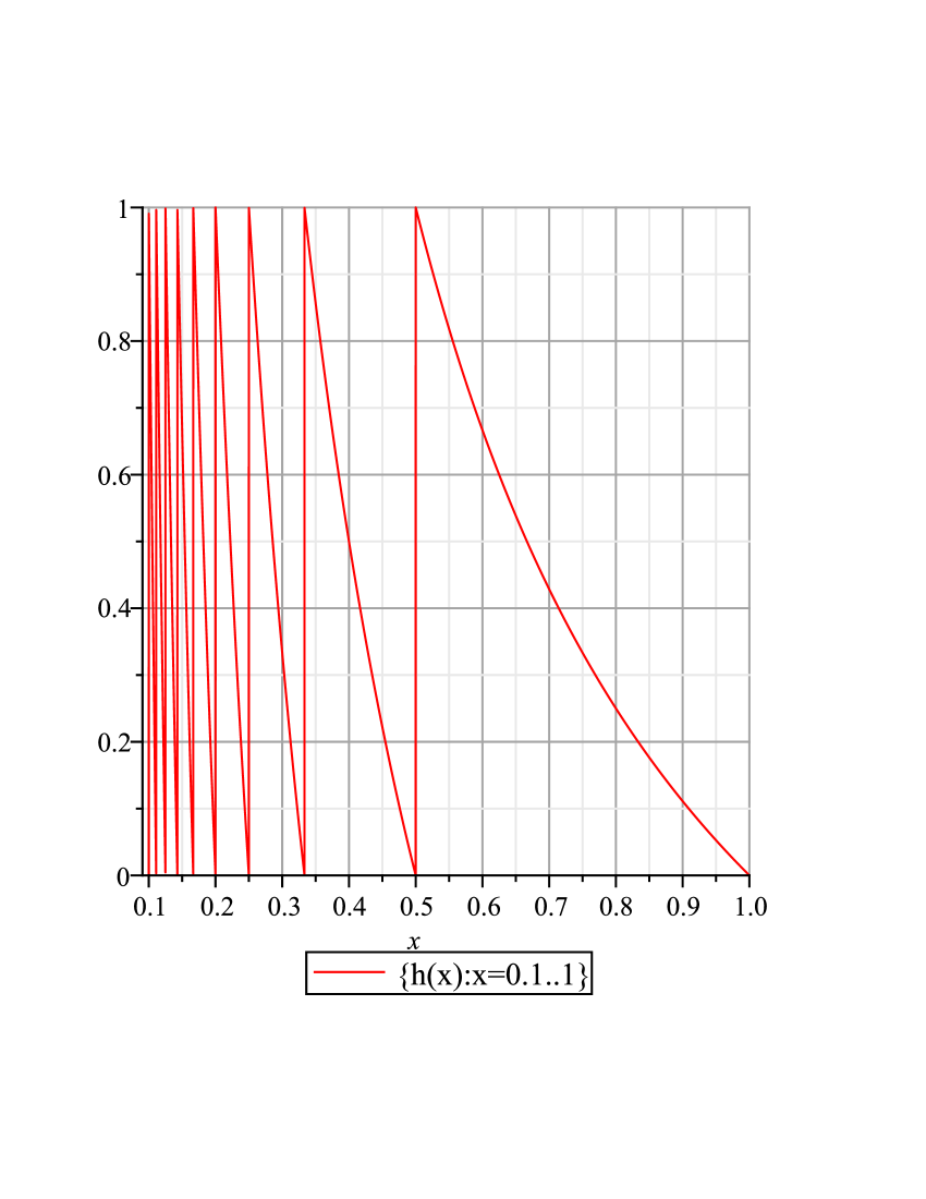
Figure 1. The Gauss Map

2.2.1. The Frobenius-Perron Transfer Operator

The Frobenius-Perron transfer operator [42, 2.4.4][31, 2.3.3][13, 1.3.1,8.2][40, 1.8,2.4] of a unit interval mapping $f(y)$ describes how a probablility density $\rho(y)$ transforms under the action of the map.

(37) $$\begin{array}[]{ll}{}[U_{f}\rho](x)&=\int\delta(x-f(y))\rho(y)\mathrm{d}y\end{array}$$

where $\delta$ is the Dirac delta function and $\theta$ is the Heaviside step function.

(38) $$\begin{array}[]{ll}\text{$\int\delta(x)\mathrm{d}x$}&=\theta(x)\\ \theta(x)&=\left\{\begin{array}[]{ll}0&x<0\\ 1&x\geqslant 0\end{array}\right.\end{array}$$

The function $f(y)$ is the map being iterated and $\rho(y)$ is some density on which the transfer operator $U$ acts. Essentially, iteration of the map transforms points to points and iteration of the transfer operator maps point densities to point densities. The Gauss-Kuzmin-Wirsing(GKW) operator is obtained by applying the transfer operator to the Guass map. [44, 2] [50] [46]

(39) $$\begin{array}[]{ll}{}[U_{h}\rho](x)&=\sum_{n=1}^{\infty}\frac{\rho\left(\frac{1}{n+x}\right)}{(n+x)^{2}}\end{array}$$

By changing the variables and order of integration in (65) an operator equation for $\zeta(s$) is obtained.

(40) $$\begin{array}[]{ll}\zeta(s)&=\frac{s}{s-1}-s\int_{0}^{1}x[U_{h}x^{s-1}]\mathrm{d}x\\ &=\frac{s}{s-1}-s\int_{0}^{1}x\int\delta(x-h(y))y^{s-1}\mathrm{d}y\mathrm{d}x\\ &=\frac{s}{s-1}-s\int_{0}^{1}x\int\delta(x-\left(y^{-1}-\left\lfloor y^{-1}\right\rfloor\right))y^{s-1}\mathrm{d}y\mathrm{d}x\\ &=\frac{s}{s-1}-s\int_{0}^{1}x\sum_{n=1}^{\infty}\frac{\left(\frac{1}{n+x}\right)^{s-1}}{(n+x)^{2}}\mathrm{d}x\end{array}$$

An operator similiar to (39) is

(41) $$\begin{array}[]{ll}{}[S_{h}\rho](x)&=\sum_{n=1}^{\infty}\rho\left(\frac{1}{n}\right)-\rho\left(\frac{1}{n+x}\right)\end{array}$$

The action of $[U_{h}\rho](x)$ on the identity function $x\rightarrow x$ is given by

(42) $$\begin{array}[]{ll}{}[U_{h}x](x)&=\sum_{n=1}^{\infty}\frac{\frac{1}{n+x}}{(n+x)^{2}}\\ &=\sum_{n=1}^{\infty}\frac{1}{(n+x)^{3}}\\ &=-\frac{\Psi^{(2)}(x+1)}{2}\\ &=\frac{{}_{4}F_{3}\left(\begin{array}[]{llll}1&x+1&x+1&x+1\\ &x+2&x+2&x+2\end{array}\right)}{(x+1)^{3}}\end{array}$$

where $\Psi^{(n)}(x)$ is the polygamma function (122). The area under the curve of $[U_{h}x](x)$ is

(43) $$\begin{array}[]{l}\int_{0}^{1}\end{array}[U_{h}x](x)\mathrm{d}x=\begin{array}[]{l}\int_{0}^{1}\end{array}-\frac{\Psi^{(2)}(x+1)}{2}\mathrm{d}x=\frac{1}{2}$$

The identity action of $[S_{h}\rho](x)$ is

(44) $$\begin{array}[]{ll}{}[S_{h}x](x)&=\sum_{n=1}^{\infty}\frac{1}{n}-\frac{1}{n+x}\\ &=\gamma+\Psi(x+1)\end{array}$$

where $\gamma$ is Euler’s constant

(45) $$\begin{array}[]{ll}\gamma&=\lim_{n\rightarrow\infty}\sum_{k=1}^{n}\frac{1}{k}-\ln(n)\\ &=\lim_{s\rightarrow 1}\zeta(s)-\frac{1}{s-1}\\ &=\lim_{s\rightarrow 1}\zeta(s)+\int_{1}^{\infty}h(x)x^{s-1}\mathrm{d}x\\ &=\lim_{s\rightarrow 1}\frac{1}{s-1}-s\int_{0}^{1}h(x)x^{s-1}\mathrm{d}x+\int_{1}^{\infty}h(x)x^{s-1}\mathrm{d}x\\ &=1-\int_{0}^{1}h(x)\mathrm{d}x\\ &\approx 0.57721566490153286060651209\end{array}$$

and the area under its curve is given by

(46) $$\begin{array}[]{ll}\int_{0}^{1}[S_{h}x](x)\mathrm{d}x&=\int_{0}^{1}\gamma+\Psi(x+1)\mathrm{d}x=1-\gamma\end{array}$$

2.2.2. Piecewsise Integration of $h(x)$

The Guass map $h(x)\in\Omega_{h}$ is piecewise monotone [40, 2.1] between the points of $\partial\Omega_{h}$, and thus partitions the unit interval infinite covering set of decreasing open intervals seperated by $\partial\Omega_{h}$. [13, 5.7.1] Let $I_{n}$ be an infinite set of open intervals

(47) $$\begin{array}[]{ll}I_{n}&=\left\{\begin{array}[]{ll}(1,\infty)&n=0\\ \left(\frac{1}{n+1},\frac{1}{n}\right)&0<n<\infty\\ (0,0)=\emptyset&n=\infty\end{array}\right.\end{array}$$

It is easy to see that

(48) $$\begin{array}[]{lll}\Omega_{h}\cup\partial\Omega_{h}=&[0,1]&=\text{$\bigcup_{n=1}^{\infty}I_{n}$}\\ &[0,\infty]&=\text{$\bigcup_{n=0}^{\infty}I_{n}$}\end{array}$$

Define the Gauss map partition $h_{n}(x)$ where $\{h_{n}(x)\neq 0:x\in I_{n}\}$ as a piecewise step function

(49) $$\begin{array}[]{ll}h_{n}(x)&=\left\{\begin{array}[]{ll}\frac{1-xn}{x}&\frac{1}{n+1}<x<\frac{1}{n}\\ 0&\operatorname{otherwise}\end{array}\right.\\ &=\left(\frac{1-xn}{x}\right)\left(\theta\left(\frac{xn+x-1}{n+1}\right)-\theta\left(\frac{xn-1}{n}\right)\right)\end{array}$$

where $\theta(t)$ is the Heaviside step function (38). We can reassemble all of the $\{h_{n}(x)\}_{n=1}^{\infty}$ to recover $h(x$)

(50) $$\begin{array}[]{ll}h(x)&=\sum_{n=1}^{\infty}h_{n}(x)\\ &=\sum_{n=1}^{\infty}\left(\frac{1-xn}{x}\right)\left(\theta\left(\frac{xn+x-1}{n+1}\right)-\theta\left(\frac{xn-1}{n}\right)\right)\end{array}$$

where only one of the $h_{n}(x)$ is $\operatorname{nonzero}$ for each $x$. By setting $n=\left\lfloor\frac{1}{x}\right\rfloor$ in (49) we get

(51) $$\begin{array}[]{ll}h(x)&=\left\{\begin{array}[]{ll}\frac{1-x\left\lfloor\frac{1}{x}\right\rfloor}{x}&\frac{1}{\left\lfloor\frac{1}{x}\right\rfloor+1}<x<\frac{1}{\left\lfloor\frac{1}{x}\right\rfloor}\\ 0&\operatorname{otherwise}\end{array}\right.\\ &=\left(\frac{1-x\left\lfloor\frac{1}{x}\right\rfloor}{x}\right)\left(\theta\left(\frac{x\left\lfloor\frac{1}{x}\right\rfloor+x-1}{\left\lfloor\frac{1}{x}\right\rfloor+1}\right)-\theta\left(\frac{x\left\lfloor\frac{1}{x}\right\rfloor-1}{\left\lfloor\frac{1}{x}\right\rfloor}\right)\right)\end{array}$$

Define the partitioned integral operator $\left[Pf(x);x\right](n)$ by

(52) $$\begin{array}[]{lllll}\text{$\left[Pf(x);x\right](n)$}&=\text{$\left[Pf(x)\right](n)$}&=\left[Pf\right](n)&=\int_{\frac{1}{n+1}}^{\frac{1}{n}}f(x)\mathrm{d}x&=\int_{I_{n}}f(x)\mathrm{d}x\end{array}$$

where by convention we have

(53) $$\begin{array}[]{llll}\left[Pf(x)\right](0)&=\lim_{n\rightarrow 0^{+}}\int_{I_{n}}f(x)\mathrm{d}x&=\int_{1}^{\infty}f(x)\mathrm{d}x&\\ \left[Pf(x)\right](\infty)&=\lim_{n\rightarrow\infty}\int_{I_{n}}f(x)\mathrm{d}x&=\int_{0}^{0}f(x)\mathrm{d}x&=0\end{array}$$

Thus

(54) $$\begin{array}[]{lll}\int_{0}^{1}f(x)\mathrm{d}x&=\sum_{n=1}^{\infty}\left[Pf(x)\right](n)&=\sum_{n=1}^{\infty}\int_{I_{n}}f(x)\mathrm{d}x\\ \int_{0}^{\infty}f(x)\mathrm{d}x&=\sum_{n=0}^{\infty}\left[Pf(x)\right](n)&=\sum_{n=0}^{\infty}\int_{I_{n}}f(x)\mathrm{d}x\end{array}$$

Each interval $I_{n}$ has the length

(55) $$\begin{array}[]{ll}\ell I_{n}&=\left[P1\right](n)\\ &=\int_{\frac{1}{n+1}}^{\frac{1}{n}}1\mathrm{d}x\\ &=\frac{1}{n}-\frac{1}{n+1}\\ &=\frac{1}{n(n+1)}\end{array}$$

The elements $n(n+1)$ are known as the oblong numbers [15, A002378]. It is seen, together with (44), that

(56) $$\begin{array}[]{ll}|\Omega_{h}|&=\int_{0}^{1}1\mathrm{d}x\\ &=\sum_{n=1}^{\infty}\ell I_{n}\\ &=\sum_{n=1}^{\infty}\frac{1}{n(n+1)}\\ &=[S_{h}x](1)\\ &=\gamma+\Psi(2)\\ &=1\end{array}$$

The piecewise integral operator $\left[Pf(x);x\right](n)$ can be used to calculate the area under the curve of $h(x)$ which is also equal to the area under the curve of $[S_{h}x](x)$. Let the length of the $n$-th component $h_{n}(x)$ be denoted by

(57) $$\begin{array}[]{ll}\ell h_{n}&=\left[Ph(x);x\right](n)\\ &=\int_{I_{n}}h(x)\mathrm{d}x\\ &=\int_{I_{n}}h_{n}(x)\mathrm{d}x\\ &=\int_{0}^{1}h_{n}(x)\mathrm{d}x\\ &=\frac{\ln(n+1)n+\ln(n+1)-\ln(n)n-\ln(n)-1}{n+1}\end{array}$$

Regarding $h(x)$ as a fractal string $\mathcal{L}_{h}=\{h_{n}(x)\}_{n=1}^{\infty}$ its length $|\mathcal{L}_{h}|$ is given by

(58) $$\begin{array}[]{ll}\text{$|\mathcal{L}_{h}|$}&=\int_{0}^{1}h(x)\mathrm{d}x\\ &=\sum_{n=1}^{\infty}\ell h_{n}\\ &=\sum_{n=1}^{\infty}\frac{\ln(n+1)n+\ln(n+1)-\ln(n)n-\ln(n)-1}{n+1}\\ &=\int_{0}^{1}[S_{h}x](x)\mathrm{d}x\\ &=\int_{0}^{1}\gamma+\Psi(x+1)\mathrm{d}x\\ &=1-\gamma\end{array}$$

If $n=0$ in (48) we get the interval $\left.I_{0}=\left(\frac{1}{1},\frac{1}{0}\right)=(1,\infty\right)$ and

(59) $$\begin{array}[]{ll}\ell h_{0}=&\int_{I_{0}}h(x)\mathrm{d}x=\int_{1}^{\infty}\frac{1}{x}\mathrm{d}x=\infty\end{array}$$

but if we choose a finite cutoff then

(60) $$\begin{array}[]{ll}\int_{1}^{y}h(x)\mathrm{d}x&=\int_{1}^{y}\frac{1}{x}\mathrm{d}x\\ &=\ln(y)\end{array}$$

and

(61) $$\begin{array}[]{l}\int_{1}^{\infty}\end{array}\frac{\ln(y)}{y^{n}}\mathrm{d}y=\frac{1}{(n-1)^{2}}$$

thus

(62) $$\begin{array}[]{ll}\sum_{n=2}^{\infty}\begin{array}[]{l}\int_{1}^{\infty}\end{array}\frac{\int_{1}^{y}h(x)\mathrm{d}x}{y^{n}}\mathrm{d}y&=\sum_{n=2}^{\infty}\begin{array}[]{l}\int_{1}^{\infty}\end{array}\frac{\int_{1}^{y}\frac{1}{x}\mathrm{d}x}{y^{n}}\mathrm{d}y\\ &=\sum_{n=2}^{\infty}\begin{array}[]{l}\int_{1}^{\infty}\end{array}\frac{\ln(y)}{y^{n}}\mathrm{d}y\\ &=\sum_{n=2}^{\infty}\frac{1}{(n-1)^{2}}\\ &=\zeta(2)\\ &=\frac{\pi^{2}}{6}\end{array}$$

2.2.3. The Mellin Transform

The Mellin transform [36, II.10.8][3, 3.6] is defined as

(63) $$\begin{array}[]{ll}M^{(a,b)}_{x\rightarrow s}f(x)&=\int_{a}^{b}f(x)x^{s-1}\mathrm{d}x\end{array}$$

where the usual definition of the Mellin transform is $M^{(0,\infty)}_{x\rightarrow s}f(x)$. Somewhat incredibly, by taking the Mellin transformation of $h(x)$ over the unit interval, we get an analytic continuation of $\zeta(s)$ which is convergent when $s$ is not equal to a negative integer, $0$, or $1$. When $s$ is a negative integer or 0 the limit or analytic continuation must be taken since the series is formally divergent at these points, and of course the series $s=1$ diverges. [45] [44] [43]

(64) $$\begin{array}[]{ll}M_{x\rightarrow s}^{I_{n}}h(x)&=\left[Ph(x)x^{s-1};x\right](n)\\ &=\int_{\frac{1}{n+1}}^{\frac{1}{n}}\left(\frac{1}{x}-\left\lfloor\frac{1}{x}\right\rfloor\right)x^{s-1}\mathrm{d}x\\ &=-\frac{n(n+1)^{-s}+s(n+1)^{-s}-n^{1-s}}{s(s-1)}\end{array}$$

(65) $$\begin{array}[]{ll}\zeta(s)&=\frac{1}{s-1}-sM_{x\rightarrow s}^{(0,1)}h(x)\\ &=\frac{1}{s-1}-s\int_{0}^{1}h(x)x^{s-1}\mathrm{d}x\\ &=\frac{1}{s-1}-s\int_{0}^{1}\left(\frac{1}{x}-\left\lfloor\frac{1}{x}\right\rfloor\right)x^{s-1}\mathrm{d}x\\ &=\frac{s}{s-1}-s\sum_{n=1}^{\infty}M_{x\rightarrow s}^{I_{n}}h(x)\\ &=\frac{s}{s-1}-s\sum_{n=1}^{\infty}-\frac{n(n+1)^{-s}+s(n+1)^{-s}-n^{1-s}}{s(s-1)}\end{array}$$

The term $\frac{1}{s-1}$ changes to $\frac{s}{s-1}=\text{$\frac{1}{s-1}-(-1)$}$ by subtracting the residue [47, 10.41][48, 6.1] of

(66) $$M_{x\rightarrow s}^{I_{0}}h(x)=\int_{I_{0}}h(x)x^{s-1}\mathrm{d}x=\int_{1}^{\infty}\frac{x^{s-1}}{x}\mathrm{d}x=-\frac{1}{s-1}$$

at the singular point $s=1$, which happens to coincide with $\sum_{s=2}^{\infty}\frac{-\frac{1}{s-1}}{s}$

(67) $$\begin{array}[]{ll}\operatorname{Res}\left(\int_{1}^{\infty}\frac{x^{s-1}}{x}\mathrm{d}x;1\right)&=\operatorname{Res}\left(-\frac{1}{s-1};1\right)\\ &=\sum_{s=2}^{\infty}-\frac{\frac{1}{s-1}}{s}\\ &=-1\end{array}$$

2.3. The Harmonic Sawtooth w(x)

Define the harmonic sawtooth map $w(x)\in\Omega_{h}\backslash\partial\Omega_{h}$ which shares the same domain and boundary as the Gauss map $h(x)$ to which it is similiar, and also has the property that its Mellin transform is the (appropriately scaled) zeta function. The $n$-th component $w_{n}(x)$ is defined over the $n$-th interval $I_{n}$

(68) $$\begin{array}[]{ll}w_{n}(x)&=\left\{\begin{array}[]{ll}n(xn+x-1)&\frac{1}{n+1}<x<\frac{1}{n}\\ 0&\operatorname{otherwise}\end{array}\right.\\ &=n(xn+x-1)\left(\theta\left(\frac{xn+x-1}{n+1}\right)-\theta\left(\frac{xn-1}{n}\right)\right)\end{array}$$

and by the substitution $n\rightarrow\left\lfloor\frac{1}{x}\right\rfloor$ we have

(69) $$\begin{array}[]{ll}w(x)&=\sum_{n=1}^{\infty}w_{n}(x)\\ &=\sum_{n=1}^{\infty}n(xn+x-1)\left(\theta\left(\frac{xn+x-1}{n+1}\right)-\theta\left(\frac{xn-1}{n}\right)\right)\\ &=\left\lfloor\frac{1}{x}\right\rfloor\left(x\left\lfloor\frac{1}{x}\right\rfloor+x-1\right)\end{array}$$

Unlike $h(x)$ which is nonzero outside of $|x|>1$, the (harmonic) sawtooth map has $w(x)=0\forall|x|>1$.

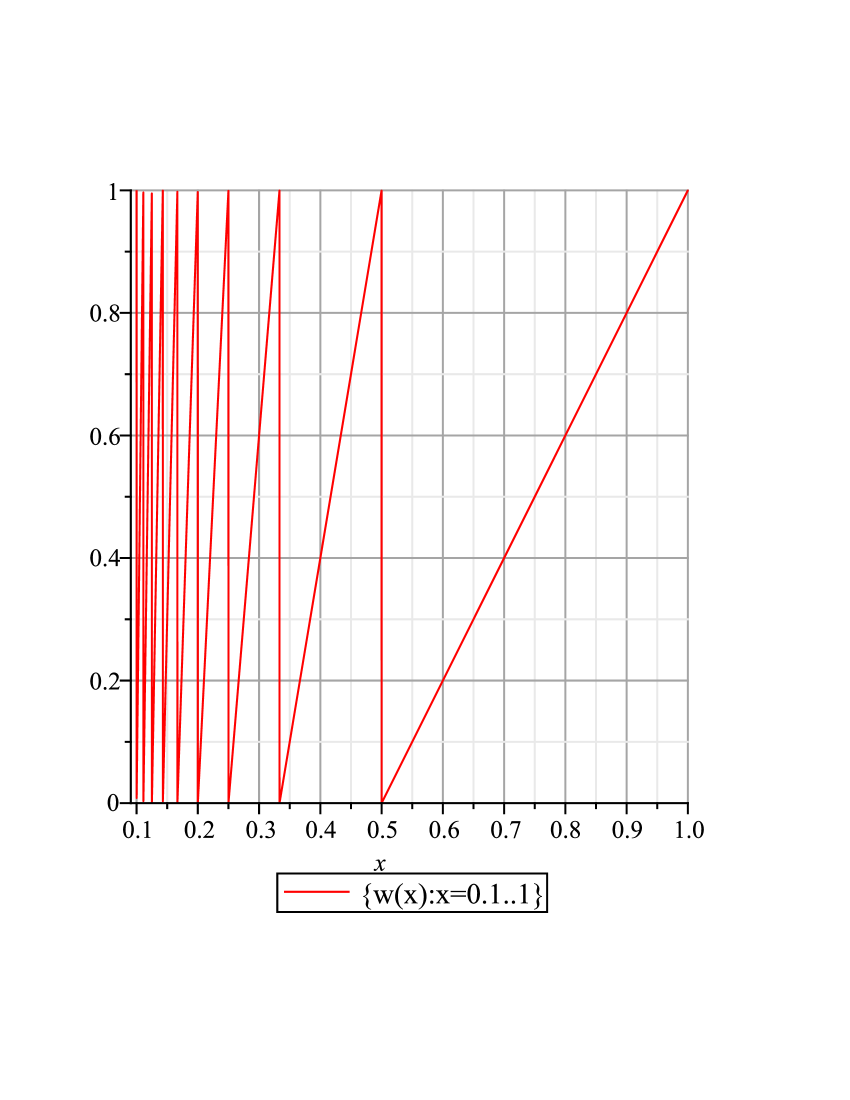
Figure 2. The Harmonic Sawtooth

The length of each component of $w(x)$ is

(70) $$\begin{array}[]{ll}\ell w_{n}&=\left[Pw(x);x\right](n)\\ &=\int_{I_{n}}w(x)\mathrm{d}x\\ &=\frac{1}{2(n+1)n}\end{array}$$

So that the total length of the harmonic sawtooth string $\mathcal{L}_{w}$ is

(71) $$\begin{array}[]{ll}|\mathcal{L}_{w}|&=\int_{0}^{1}w(x)\mathrm{d}x\\ &=\sum_{n=1}^{\infty}\ell w_{n}\\ &=\sum_{n=1}^{\infty}\frac{1}{2(n+1)n}\\ &=\frac{1}{2}\end{array}$$

The infinite set of Mellin transforms of $w_{n}(x)$

(72) $$\begin{array}[]{ll}M_{x\rightarrow s}^{I_{n}}w(x)&=M_{x\rightarrow s}^{(0,1)}w_{n}(x)\\ &=\left[Pw(x)x^{s-1};x\right](n)\\ &=\int_{\frac{1}{n+1}}^{\frac{1}{n}}n(xn+x-1)x^{s-1}\mathrm{d}x\\ &=\int_{0}^{1}n(xn+x-1)\left(\theta\left(\frac{xn+x-1}{n+1}\right)-\theta\left(\frac{xn-1}{n}\right)\right)x^{s-1}\mathrm{d}x\\ &=-\frac{n(n+1)^{-s}+s(n+1)^{-s}-n^{1-s}}{s(s-1)}\end{array}$$

are summed to get an expression for $\{\zeta(s):\mathfrak{R}(s)\not\in\mathbbm{N}_{0^{-}}\}$

(73) $$\begin{array}[]{ll}\zeta(s)&=s\frac{s+1}{s-1}\int_{0}^{1}\left\lfloor\frac{1}{x}\right\rfloor\left(x\left\lfloor\frac{1}{x}\right\rfloor+x-1\right)x^{s-1}\mathrm{d}x\\ &=\sum_{n=1}^{\infty}s\frac{s+1}{s-1}M_{x\rightarrow s}^{I_{n}}w(x)\\ &=\sum_{n=1}^{\infty}s\frac{s+1}{s-1}\int_{\frac{1}{n+1}}^{\frac{1}{n}}n(xn+x-1)x^{s-1}\mathrm{d}x\\ &=\sum_{n=1}^{\infty}s\frac{s+1}{s-1}\left(-\frac{n(n+1)^{-s}+s(n+1)^{-s}-n^{1-s}}{s(s-1)}\right)\\ &=\sum_{n=1}^{\infty}\frac{n(n+1)^{-s}-n^{1-s}+sn^{-s}}{s-1}\end{array}$$

2.4. The Prime Numbers

Let $\mathbbm{P}=\{2,3,5,7,11,13,17,19,23,29,\ldots\}$ denote the set of prime numbers and $\mathbbm{N}_{1}=\{1,2,\ldots\}$ and $\mathbbm{N}_{0}=\{0,1,2,\ldots\},\mathbbm{N}=\{\ldots,-2,-1,0,1,2,\ldots\}$ be the set of positive, non-negative, and signed integers.

2.4.1. The Prime Counting Function: $\pi(x)$

The prime counting function $\pi(x)$ counts the number of primes less than a given number. It can written as

(74) $$\begin{array}[]{ll}\pi(x)&=\sum_{p<x}^{p\in\mathbbm{P}}1\end{array}$$

which is essentially a step function which increases by 1 for each prime. [9, 15.11]

2.4.2. von Mangoldt and Chebyshev’s Functions: $\Lambda(x),\theta(x),\text{$\psi(x)$}$

Chebyshev’s function of the first kind $\theta(x)$ is the sum of the logarithm of all primes $\leqslant x$

(75) $$\begin{array}[]{ll}\theta(x)&=\sum_{k=1}^{\pi(x)}\ln(p_{k})\\ &=\ln\left(\sum_{k=1}^{\pi(x)}p_{k}\right)\end{array}$$

where $p_{k}\in\mathbbm{P}$ is the $k$-th prime. [7, 4.4] The generalization of $\pi(x)$ is the Chebyshev function of the second kind

(76) $$\begin{array}[]{ll}\psi(x)&=\sum_{p^{r}\leqslant x}^{\{p\in\mathbbm{P},r\in\mathbbm{N}_{1}\}}\ln(p)\\ &=\sum_{k=1}^{\left\lfloor\log_{2}(x)\right\rfloor}\theta(x^{\frac{1}{k}})\\ &=\ln(\operatorname{lcm}(1,2,3,\ldots,\left\lfloor x\right\rfloor))\\ &=\sum^{n\leqslant x}_{n}\Lambda(n)\\ &=x-\frac{\ln(1-x^{-2})}{2}-\ln(2\pi)-\sum^{\zeta(\rho)=0}_{\rho}\frac{x^{\rho}}{\rho}\forall\mathcal{I}(\rho)\neq 0\end{array}$$

where the first sum ranges over the primes $p\in\mathbbm{P}$ and positive integers $r$ and the sum over $\rho$ is von Mangoldt’s formula where $\rho$ ranges over the non-trivial roots of $\zeta(s)$ in increasing order. The function $\operatorname{lcm}(\ldots.)$ is the least common multiple, and $\Lambda(x)$ is the von Mangoldt function.

(77) $$\begin{array}[]{ll}\Lambda(x)&=\left\{\begin{array}[]{ll}\ln(p)&\{n=p^{k}:p\in\mathbbm{P},k\in\mathbbm{N}_{1}\}\\ 0&\operatorname{otherwise}\end{array}\right.\\ &=\ln\left(\frac{\operatorname{lcm}(1,2,\ldots,n)}{\operatorname{lcm}(1,2,\ldots,n-1)}\right)\end{array}$$

$\Lambda(s)$ is related to $\zeta(s)$ by

(78) $$-\frac{\frac{\mathrm{d}}{\mathrm{d}s}\zeta(s)}{\zeta(s)}=\sum_{n=1}^{\infty}\frac{\Lambda(n)}{n^{s}}\forall\mathcal{R}(s)>1$$

Chebyshev proved that $\pi(x),\theta(x),\operatorname{and}\text{$\psi(x)$}$  have the same scaled asymptotic limit.

(79) $$\lim_{x\rightarrow\infty}\frac{\pi(x)}{\left(\frac{x}{\ln(x)}\right)}=\lim_{x\rightarrow\infty}\frac{\psi(x)}{x}=\lim_{x\rightarrow\infty}\frac{\theta(x)}{x}=1$$

[18, 1.3] [17, I.4] [7, 4.3-4.4&3.1-3.2] [8] [9, 15.11]. Note that [9] incorrectly defines $\psi(x)$ as $\ln(\gcd(\ldots)).$

3. Analytic Continuation

3.1. Continuation of ${}_{n+1}F_{n}$ Near Unit Argument

The continuation formula for Gauss’s hypergeometric function ${}_{2}F_{1}$ near unit argument is well known

(80) $$\begin{array}[]{ll}\frac{\Gamma(a_{1})\Gamma(a_{2})}{\Gamma(b_{1})}_{2}F_{1}\left(\begin{array}[]{ll}a_{1}&a_{2}\\ b_{1}&\end{array}|z\right)&=\sum_{n=0}^{\infty}\frac{(-1)^{n}(1-z)^{n}}{n!}\frac{\Gamma(a_{1}+n)\Gamma(a_{2}+n)\Gamma(s_{1}-n)}{\Gamma(a_{1}+s_{1})\Gamma(a_{2}+s_{1})}\\ &+(1-z)^{s_{1}}\sum_{n=0}^{\infty}\frac{(-1)^{n}(1-z)^{n}}{n!}\frac{\Gamma(a_{1}+s_{1}+n)\Gamma(a_{2}+s_{1}+n)\Gamma(-s_{1}-n)}{\Gamma(a_{1}+s_{1})\Gamma(a_{2}+s_{1})}\end{array}$$

where $s_{1}=b_{1}-a_{1}-a_{2}$ is the balance (117) of ${}_{2}F_{1}$ which must not be equal to an integer, that is, ${}_{2}F_{1}$ cannot be $s_{1}$-balanced. A function is said to be $k$-balanced only when $k$ is an integer. When $\mathcal{R}(s_{1})>0$ the value at $z=1$ is finite and given by the Gaussian summation formula

(81) $$\begin{array}[]{ll}\frac{{}_{2}F_{1}\left(\begin{array}[]{ll}a_{1}&a_{2}\\ b_{1}&\end{array}\right)}{\Gamma(b_{1})}&=\frac{\Gamma(b_{1}-a_{1}-a_{2})}{\Gamma(b_{1}-a_{1})\Gamma(b_{1}-a_{2})}\\ &=\frac{\Gamma(s_{1})}{\Gamma(a_{1}+s_{1})\Gamma(a_{2}+s_{1})}\end{array}$$

It is obvious that $\lim_{t\rightarrow 1}\operatorname{Li}_{1}^{F}(t)=\lim_{t\rightarrow 1}\text{${}_{2}F_{1}\left(\begin{array}[]{ll}1&1\\ 2&\end{array}|t\right)=\zeta^{F}(1)$}=\infty$ is $0$-balanced and of course equal to the divergent harmonic series so the continuation formula does not apply. However, Bühring and Srivastava [6][5] generalized this relation to all ${}_{n+1}F_{n}$ by expanding (81) as a series then interchanging the order of summations to derive a recurrence with respect to $n$

(82) $$\begin{array}[]{ll}{}_{n+1}F_{n}\left(\begin{array}[]{l}a_{1},\ldots,a_{n+1}\\ b_{1},\ldots,b_{n}\end{array}|t\right)&=\frac{\Gamma(b_{n})\Gamma(b_{n-1})}{\Gamma(a_{n+1})\Gamma(b_{n}+b_{n-1}-a_{n+1})}\\ &\cdot\sum_{m=0}^{\infty}\frac{(b_{n}-a_{n+1})_{m}(b_{n-1}-a_{n-1})_{m}}{(b_{n}+b_{n-1}-a_{n+1})_{m}m!}_{n}F_{n-1}\left(\begin{array}[]{l}a_{1},\ldots,a_{n}\\ b_{1},\ldots,b_{n-2},b_{n-1}+b_{n}-a_{n+1}+m\end{array}|t\right)\end{array}$$

which is valid $\forall\{\mathcal{R}(a_{i})>0:1\leqslant i\leqslant n+1\}$. The $m$-th term of the summand in (82) is contiguous (4.1.2) to the ($m-1$)-th and ($m+1$)-th terms and thus a linear relationship can always be found between neighboring terms.

3.2. The Continuation of $\operatorname{Li}_{n}^{F}(t)\operatorname{and}\zeta^{F}(n)$ via Contiguous Functions

There are 4 functions contiguous (4.1.2) to $\operatorname{Li}_{n}^{F}(t)$, only 3 of them are unique, and just 1 of them is interesting. The functions are obtained by shifting one of the numerator parameters $a_{i}\pm 1$ or shifting one of the denominator parameters $b_{i}\pm 1$. Shifting any of the $a$ parameters or any of the $b$ parameters will suffice since they are all equal and ${}_{p}F_{q}$ is invariant with respect to the ordering of parameters. Let $\vec{c}^{+}_{n}$ and $\vec{c}^{-}_{n}$ denote the parameter vector $\vec{c}_{n}$ where one element is shifted up or down by $1$.

(83) $$\begin{array}[]{ll}\vec{c}^{+}_{n}&=\vec{c}_{n-1},c+1=\underbrace{c,\ldots,c}_{n-1},c+1\\ \vec{c}^{-}_{n}&=\vec{c}_{n-1},c-1=\underbrace{c,\ldots,c}_{n-1},c-1\end{array}$$

For example, $\vec{4}_{3}^{+}=4,4,5$. Two of the four functions contiguous to $\operatorname{Li}_{n}^{F}(t)$ are identical

(84) $$\begin{array}[]{ll}{}_{n+1}F_{n}\left(\begin{array}[]{l}\vec{1}^{+}_{n+1}\\ \vec{2}_{n}\end{array}|t\right)t&=_{n+1}F_{n}\left(\begin{array}[]{l}\vec{1}_{n+1}\\ \vec{2}^{-}_{n}\end{array}|t\right)t=\operatorname{Li}_{n-1}^{F}(t)\end{array}$$

Shifting any $a_{i}$ up is equivalent to shifting any $b_{i}$ down, both operations take $\operatorname{Li}_{n}^{F}(t)$ to $\operatorname{Li}_{n-1}^{F}(t)$. Shifting any $a_{i}$ down results in the identity function since it puts a $0$ in the numerator.

(85) $${}_{n+1}F_{n}\left(\begin{array}[]{l}\vec{1}^{-}_{n+1}\\ \vec{2}_{n}\end{array}|t\right)t=t$$

Thus, the only interesting function continguous to $\operatorname{Li}_{n}^{F}(t)$ is obtained by shifting one of the denominator parameters up. Let this function be denoted by $\operatorname{Li}_{n}^{F+1}(t)$

(86) $$\begin{array}[]{ll}\text{$\operatorname{Li}_{n}^{F+1}(t)$}=_{n+1}F_{n}\left(\begin{array}[]{l}\vec{1}_{n+1}\\ \vec{2}^{+}_{n}\end{array}|t\right)&=\left\{\begin{array}[]{ll}I_{0}\left(2\sqrt{t}\right)-\frac{1}{\sqrt{t}}I_{1}\left(2\sqrt{t}\right)&n=0\\ \frac{e^{t}}{t}-\frac{1}{t}-1&n=1\\ (-1)^{n}\left(1-\frac{\operatorname{Li}_{1}(t)}{t}+\sum_{k=1}^{n-1}(-1)^{k+1}\operatorname{Li}_{k}(t)\right)&n\geqslant 2\end{array}\right.\end{array}$$

where $I_{n}(x)$ is a modified Bessel function of the first kind [34, 65] [10, 6.9.1]

(87) $$\begin{array}[]{ll}I_{n}(x)&=\frac{x^{n}}{\Gamma(n+1)2^{n}}_{0}F_{1}\left(\begin{array}[]{l}\\ n+1\end{array}|\frac{x^{2}}{4}\right)\end{array}$$

Before applying (82), the notation will be simplified by extending (83) so that repeated shifts can be written more easily

(88) $$\begin{array}[]{ll}\vec{c}^{+j}_{n}&=\vec{c}_{n-1},c+j=\underbrace{c,\ldots,c}_{n-1},c+j\\ \vec{c}^{-j}_{n}&=\vec{c}_{n-1},c-j=\underbrace{c,\ldots,c}_{n-1},c-j\end{array}$$

where clearly $\vec{c}^{+}_{n}=\vec{c}^{+1}_{n}$ and $\vec{c}^{-}_{n}=\vec{c}^{-1}_{n}$. The goal is to extend $\operatorname{Li}_{n}^{F+1}(t)$ to all $\operatorname{Li}_{n}^{F+m}(t)$ by repeated application of $\vec{c}^{+1}_{n}$. Applying (82) to (13) gives the continuation of $\operatorname{Li}_{n}^{F}(t)\rightarrow\operatorname{Li}_{n+1}^{F}(t)\forall n\geqslant 1$ by setting $a_{1\ldots n+1}=\vec{1}_{n+1}$ and $b_{1\ldots n}=\vec{2}_{n}$ which results in

(89) $$\begin{array}[]{ll}\operatorname{Li}_{n}^{F}(t)&={{}_{n+1}F_{n}}\left(\begin{array}[]{l}\vec{1}_{n+1}\\ \vec{2}_{n}\end{array}|t\right)t\forall n\geqslant 0\\ &=t\sum_{m=0}^{\infty}\left(\frac{{}_{n}F_{n-1}\left(\begin{array}[]{l}\vec{1}_{n}\\ \vec{2}_{n-2},3+m\end{array}|t\right)}{(m+1)(m+2)}\right)\forall n\geqslant 2\\ &=t\sum_{m=0}^{\infty}\left(\frac{{}_{n}F_{n-1}\left(\begin{array}[]{l}\vec{1}_{n}\\ \vec{2}^{+m+1}_{n-1}\end{array}|t\right)}{(m+1)(m+2)}\right)\forall n\geqslant 2\end{array}$$

since

(90) $$\frac{\Gamma(b_{n})\Gamma(b_{n-1})}{\Gamma(a_{n+1})\Gamma(b_{n}+b_{n-1}-a_{n+1})}=\frac{\Gamma(2)\Gamma(2)}{\Gamma(1)\Gamma(2+2-1)}=\frac{1}{2}$$

and

(91) $$\frac{(b_{n}-a_{n+1})_{m}(b_{n-1}-a_{n-1})_{m}}{(b_{n}+b_{n-1}-a_{n+1})m!}=\frac{(1)_{m}(1)_{m}}{(2+2-1)_{m}m!}=\frac{2}{(m+1)(m+2)}$$

The denominator parameters $\vec{2}^{+1+m}_{n-1}$ in (89) are simply

(92) $$\begin{array}[]{lll}\vec{2}^{+1+m}_{n-1}&=\vec{2}_{n-2},3+m&=\underbrace{2,\ldots,2}_{n-2},3+m\end{array}$$

The numbers ($m+1)(m+2$) are known as the oblong numbers, [15, A002378]. By simply setting $t=1$ in (89) we get the continuation from $\zeta^{F}(n)\rightarrow\zeta^{F}(n+1)\forall n\geqslant 1$

(93) $$\begin{array}[]{ll}\zeta^{F}(n)=_{n+1}F_{n}\left(\begin{array}[]{l}\vec{1}_{n+1}\\ \vec{2}_{n}\end{array}\right)&=\sum_{m=0}^{\infty}\left(\frac{{}_{n}F_{n-1}\left(\begin{array}[]{l}\vec{1}_{n}\\ \vec{2}^{+m+1}_{n-1}\end{array}\right)}{(m+1)(m+2)}\right)\forall n\geqslant 2\end{array}$$

The justification in saying that $\operatorname{Li}_{n}^{F}(t)$ and $\zeta^{F}(n)$ are continued to $\operatorname{Li}_{n+1}^{F}(t)$ and $\zeta^{F}(n+1)$ comes from the fact that the first term in the summand of the continuation (89) from $\operatorname{Li}_{n-1}^{F}(t)\rightarrow\operatorname{Li}_{n}^{F}(t$) is contiguous to  $\operatorname{Li}_{n-1}^{F}(t)$, that is, ${}_{n}F_{n-1}\left(\begin{array}[]{l}\vec{1}_{n}\\ \vec{2}^{+1}_{n-1}\end{array}|t\right)$ is contiguous to $\operatorname{Li}_{n-1}^{F}(t)=\text{${}_{n}F_{n-1}\left(\begin{array}[]{l}\vec{1}_{n}\\ \vec{2}_{n-1}\end{array}|t\right)$}$. The continuation formula (89) gives interesting answers for $n=0$ and $n=1$ which suggest an alternative to “the analytic continuation” of $\zeta\left(t\right)$ which is different from the usual $\frac{1}{1-2^{-t}}\sum_{n=0}^{\infty}(2n+1)^{-t}$. We have

(94) $$\begin{array}[]{llll}\zeta^{F}(0)&=\sum_{m=0}^{\infty}\left(\frac{{}_{0}F_{1}\left(\begin{array}[]{l}\\ m+3\end{array}\right)}{(m+1)(m+2)}\right)&&\\ &=\sum_{m=0}^{\infty}\frac{-\left(I_{m+1}\left(2\right)m+I_{m+1}\left(2\right)-I_{m}\left(2\right)\right)\Gamma\left(m+3\right)}{(m+1)(m+2)}&&\\ &=I_{0}(2)-1&&\\ &\approx 1.2795853023360&&\\ \zeta^{F}(1)&=\sum_{m=0}^{\infty}\left(\frac{{}_{1}F_{1}\left(\begin{array}[]{l}1\\ m+3\end{array}\right)}{(m+1)(m+2)}\right)&&\\ &=\sum_{m=0}^{\infty}\frac{e\left(\Gamma\left(m+3\right)-\Gamma\left(m+2,1\right)m-2\Gamma\left(m+2,1\right)\right)}{(m+1)(m+2)}&&\\ &=\operatorname{Ei}(1)-\gamma&&\\ &\approx 1.3179021514544&&\end{array}$$

where $\operatorname{Ei}(x)$ is the exponential integral [10, 6.9.2]

(95) $$\begin{array}[]{ll}\operatorname{Ei}(x)&=\gamma-\frac{\ln(x^{-1})}{2}+\frac{\ln(x)}{2}+\sum_{k=1}^{\infty}\frac{x^{k}}{k\Gamma(k+1)}\\ &=\gamma-\frac{\ln(x^{-1})}{2}+\frac{\ln(x)}{2}+x_{2}F_{2}\left(\begin{array}[]{ll}1&1\\ 2&2\end{array}|x\right)\end{array}$$

and $\Gamma\left(a,z\right)$ is the incomplete Gamma function

(96) $$\Gamma\left(a,z\right)=\Gamma\left(z\right)-\frac{z^{a}_{1}F_{1}\left(\begin{array}[]{l}a\\ a+1\end{array}|-z\right)}{a}$$

So we have the “hypergeometrically continued” values $\zeta^{F}(0)=I_{0}(2)-1$ and $\zeta^{F}(1)=\operatorname{Ei}(1)-\gamma$ whereas the “real” values are $\zeta\left(0\right)=-\frac{1}{2}$ and $\zeta\left(1\right)=\infty$. In terms of reciprocal probability we have

(97) $$\begin{array}[]{ll}\zeta^{F}\left(0\right)^{-1}&\cong 78.15\%\\ \zeta^{F}\left(1\right)^{-1}&\cong 75.88\%\end{array}$$

3.2.1. $\operatorname{Li}_{1}^{F}(t)\rightarrow\operatorname{Li}_{2}^{F}(t)$ and $\zeta_{1}^{F}(t)\rightarrow\zeta_{2}^{F}(t)$

The continuation $\zeta_{n}^{F}(t)$ from $n=1\rightarrow 2$ via (93) is straightforward

(98) $$\begin{array}[]{ll}\text{$\zeta^{F}(2)$}&=_{3}F_{2}\left(\begin{array}[]{lll}1&1&1\\ 2&2&\end{array}\right)\\ &=\sum_{m=0}^{\infty}\left(\frac{{}_{2}F_{1}\left(\begin{array}[]{ll}1&1\\ &3+m\end{array}\right)}{(m+1)(m+2)}\right)\\ &=\sum_{m=0}^{\infty}\left(\frac{\sum_{k=0}^{\infty}\frac{\Gamma(m+3)\Gamma(k+1)}{\Gamma(m+k+3)}}{(m+1)(m+2)}\right)\\ &=\sum_{m=0}^{\infty}\frac{1}{(m+1)(m+2)}\frac{(m+2)}{(m+1)}\\ &=\sum_{m=0}^{\infty}\frac{1}{(m+1)^{2}}\\ &=\frac{\pi^{2}}{6}\end{array}$$

The continuation of $\operatorname{Li}^{F}_{1}(t)$ to $\operatorname{Li}^{F}_{2}(t)$ is a bit more complicated

(99) $$\begin{array}[]{ll}\operatorname{Li}_{2}^{F}\left(t\right)&=_{3}F_{2}\left(\begin{array}[]{lll}1&1&1\\ &2&2\end{array}|t\right)\\ &=\sum_{m=0}^{\infty}\left(\frac{{}_{2}F_{1}\left(\begin{array}[]{ll}1&1\\ &m+3\end{array}|t\right)}{(m+1)(m+2)}\right)\\ &=\sum_{m=0}^{\infty}r_{2}(m,t)\end{array}$$

then $r_{2}(m,t)$ is given by

(100) $$\begin{array}[]{ll}r_{2}(m,t)&=\frac{\sum_{n=0}^{m}\frac{(-1)^{n+1}\Gamma(m+2)(\Psi(m-n+1)-\Psi(m+2))(-1)^{m}e^{\psi(m+2)}t^{n}}{\Gamma(n+2)\Gamma(m-n+1)}}{(m+1)e^{\psi(m+2)}t^{m+1}}\\ &-\frac{(t-1)^{m+1}t^{-2-m}\ln(1-t)}{m+1}\end{array}$$

so $\operatorname{Li}_{2}^{F}(t)$ is equal to

(101) $$\text{$\operatorname{Li}_{2}^{F}(t)$=}\sum_{m=0}^{\infty}\frac{\sum_{n=0}^{m}\frac{(-1)^{n+1}\Gamma(m+2)(\Psi(m-n+1)-\Psi(m+2))(-1)^{m}e^{\psi(m+2)}t^{n}}{\Gamma(n+2)\Gamma(m-n+1)}}{(m+1)e^{\psi(m+2)}t^{m+1}}-\frac{(t-1)^{m+1}t^{-2-m}\ln(1-t)}{m+1}$$

where $\psi(m)=\ln(\operatorname{lcm}(1,2,3,\ldots,m))$ is Chebyshev’s function of the 2nd kind (76) and $\Psi(m$) is the digamma function

(102) $$\Psi(x)=\frac{\mathrm{d}}{\mathrm{d}x}\ln(\Gamma(x))=\frac{\frac{\mathrm{d}}{\mathrm{d}x}\Gamma(x)}{\Gamma(x)}$$

3.2.2. $\zeta^{F}(2)\rightarrow\zeta^{F}(3)$

The continuation from $\zeta^{F}(2)$ to $\zeta^{F}(3)$ via (93) is carried out like so

(103) $$\begin{array}[]{ll}\text{$\zeta^{F}(3)$}&=_{4}F_{3}\left(\begin{array}[]{llll}1&1&1&1\\ &2&2&2\end{array}\right)\\ &=\sum_{m=0}^{\infty}\left(\frac{{}_{3}F_{2}\left(\begin{array}[]{lll}1&1&1\\ &2&3+m\end{array}\right)}{(m+1)(m+2)}\right)\\ &=\sum_{m=0}^{\infty}r_{3}(m)\end{array}$$

Each term in the summand $r_{3}(m)$ has the form $\frac{\zeta(2)}{m+1}+q_{3}(m)$ where of course $\zeta(2)=\frac{\pi^{2}}{6}$ and $q_{3}(m)$ is a rational function of $m$ which follows a 3rd order linear recurrence equation[28, 8.2] given by

(104) $$\begin{array}[]{ll}q_{3}(m)&=q_{3}\left(m+1\right)\left(m^{3}+8\hskip 2.5ptm^{2}+21\hskip 2.5ptm+18\right)\\ &+q_{3}\left(m+2\right)\left(-2\hskip 2.5ptm^{3}-20\hskip 2.5ptm^{2}-67\hskip 2.5ptm-75\right)\\ &+q_{3}\left(m+3\right)\left(m^{3}+12\hskip 2.5ptm^{2}+48\hskip 2.5ptm+64\right)\end{array}$$

(105) $$q_{3}(m)=\left\{\begin{array}[]{ll}-1&m=0\\ -\frac{5}{8}&m=1\\ -\frac{49}{108}&m=2\end{array}\right.$$

The solution to which is given by

(106) $$\begin{array}[]{ll}q_{3}(m)&=\frac{\Psi^{(1)}(m+2)-\zeta\left(2\right)}{m+1}\end{array}$$

so the summand $r_{3}(m)$ is

(107) $$\begin{array}[]{ll}r_{3}(m)&=\frac{\zeta(2)}{m+1}+q_{3}(m)=\frac{\Psi^{(1)}(2+m)}{m+1}\end{array}$$

Thus (111) is also equal to

(108) $$\begin{array}[]{ll}\zeta^{F}(3)&=\sum_{m=0}^{\infty}\frac{\Psi^{(1)}(m+2)}{m+1}\end{array}$$

Thus

(109) $$\begin{array}[]{ll}r_{3}(m)&=\frac{\Psi^{(1)}(m+2)}{m+1}\\ &=\frac{\zeta(2,m+2)}{m+1}\\ &=\frac{\pi^{2}}{6}-\sum_{k=1}^{m-1}\frac{1}{k^{2}}\\ &=\frac{\sum_{k=1}^{\infty}\frac{1}{(k+m-1)^{2}}}{m+1}\\ &=\frac{{}_{3}F_{2}\left(\begin{array}[]{lll}1&m+2&m+2\\ &m+3&m+3\end{array}\right)}{(m+1)(m+2)^{2}}\\ &=\frac{{}_{3}F_{2}\left(\begin{array}[]{lll}1&1&1\\ &2&3+m\end{array}\right)}{(m+1)(m+2)}\end{array}$$

The first 10 terms of $\{q_{3}(m):m=0\ldots 9\}$ are

(110) $$\left[-1,-\frac{5}{8},-\frac{49}{108},-\frac{205}{576},-\frac{5269}{18000},-\frac{5369}{21600},-\frac{266681}{1234800},-\frac{1077749}{5644800},-\frac{9778141}{57153600},-\frac{1968329}{12700800}\right]$$

The denominator of (110) appears to be [15, A119936], the least common multiple of denominators of the rows of a certain triangle of rationals and the numerators are [15, A007406], the numerator of $\sum_{k=1}^{n}\frac{1}{k^{2}}$ from (123) which, according to a theorem Wolstenholme, $p$ divides $\operatorname{numer}(q_{3}(p-1$)) where $p\in\mathbbm{P}$ is prime. [12] [4] [1]

3.2.3. $\zeta^{F}(3)\rightarrow\zeta^{F}(4)$

The continuation from $\zeta^{F}(3)$ to $\zeta^{F}(4)$ via (93) is given by

(111) $$\begin{array}[]{ll}\text{$\zeta^{F}(4)$}&=_{5}F_{4}\left(\begin{array}[]{lllll}1&1&1&1&1\\ 2&2&2&2&\end{array}\right)\\ &=\sum_{m=0}^{\infty}\left(\frac{{}_{4}F_{3}\left(\begin{array}[]{llll}1&1&1&1\\ &2&2&3+m\end{array}\right)}{(m+1)(m+2)}\right)\\ &=\sum_{m=0}^{\infty}r_{4}(m)\end{array}$$

The summand $r_{4}(m)$ has the form

(112) $$\begin{array}[]{ll}r_{4}(m)&=a(t,m)-b(t,m)-\frac{H(m+1)\operatorname{Li}_{2}(t)}{(m+1)t}+\frac{\operatorname{Li}_{3}(t)}{(m+1)t}\end{array}$$

where $a(t,m)$ is an $(m+1)$-th degree polynomial and $b(t,m)$ is a $(m+2)$-th degree polynomial(the determination of which is left to an excercise for the reader or the topic of another article, but is readily obtained with the help of Maple[27]), and $H(n)$ is the $n$-th Harmonic number

(113) $$\begin{array}[]{ll}H(n)&=\sum_{i=1}^{n}\frac{1}{n}\\ &=\Psi(n+1)+\gamma\\ &=\sum_{k=1}^{\infty}\frac{n}{k^{2}+kn}\\ &=\frac{n}{n+1}_{3}F_{2}\left(\begin{array}[]{lll}1&1&n+1\\ &2&n+2\end{array}\right)\end{array}$$

The polynomial $b(t,m)$ vanishes when $t=1$. An interesting set of formulas for $\zeta(4)$ is

(114) $$\begin{array}[]{ll}\zeta(4)&=\sum_{n=1}^{\infty}\frac{\Psi^{(2)}(n+1)+2\zeta(3)}{2n\left(n+1\right)}\\ &=\sum_{n=1}^{\infty}\frac{\Psi^{(2)}(n+1)+2\sum_{m=0}^{\infty}\frac{\Psi^{(1)}(m+2)}{m+1}}{2n\left(n+1\right)}\\ &=\frac{\pi^{4}}{90}\end{array}$$

4. Appendix

4.1. $\operatorname{The}\operatorname{Generalized}\operatorname{Hypergeometric}\operatorname{Function}:_{p}F_{q}$

The Pochhammer symbol is defined according to

(115) $$\begin{array}[]{ll}(n)_{k}&=\frac{\Gamma(n+k)}{\Gamma(n)}\end{array}$$

The generalized hypergeometric function [39][48, 4.1] is defined as an infinite sum of quotients of finite products of Pochhammer symbols

(116) $$\begin{array}[]{ll}\begin{array}[]{l}{}_{p}F_{q}\left(\begin{array}[]{l}a_{1},\ldots,a_{p}\\ b_{1},\ldots,b_{q}\end{array}|t\right)\end{array}&=\sum_{k=0}^{\infty}\frac{t^{k}}{k!}\frac{\prod_{i=1}^{p}(a_{i})_{k}}{\prod_{j=1}^{q}(b_{j})_{k}}\end{array}$$

The function ${}_{p}F_{q}$ is said to be $k$-balanced [5] if the sum of the denominator parameters $b_{1}\ldots b_{p}$ minus the sum of the numerator parameters $a_{1}\ldots a_{p+1}$ is an integer.

(117) $$k=\operatorname{bal}(_{p}F_{q})=\sum_{n=1}^{q}b_{n}-\sum_{n=1}^{p}a_{n}$$

The value $k$ is the characteristic exponent of the hypergeometric differential equation at unit argument which is equal to the maximum root of the corresponding indicial equation and so determines the behaviour of the function near this point. A $1$-balanced function is said to be Saalschützian. [41, 2.1.1]

4.1.1. The Differential Equation and Convergence

The function ${}_{p}F_{q}$ converges when

(118) $$\begin{array}[]{l}\left\{\begin{array}[]{lll}p\leqslant q&\forall|t|\neq\infty&\\ p=q+1&\forall|t|<1&\\ \{p=q+1:\operatorname{bal}(_{p}F_{q})\geqslant 1\}&\forall|t|=1&\\ p>q+1&\forall t=0&\end{array}\right.\end{array}$$

where $\operatorname{bal}(_{p}F_{q})=\sum_{n=1}^{q}b_{n}-\sum_{n=1}^{p}a_{n}$ is the balance of the parameters (117). The differential equation solved by ${}_{p}F_{q}\operatorname{is}\operatorname{of}\operatorname{order}\text{max(p,q+1)}$

(119) $$\left(\theta_{t}\prod_{j=1}^{q}(\theta_{t}+b_{j}-1)-t\prod_{i=1}^{p}(\theta_{t}+a_{i})\right)f(t)=0$$

where $f(t)=_{p}F_{q}\left(\begin{array}[]{l}a_{1},\ldots,a_{p}\\ b_{1},\ldots,b_{q}\end{array}|t\right)$ and $\theta_{t}=t\frac{\mathrm{d}}{\mathrm{d}t}$ is the differential operator. When $p=q+1$ (119) has the form

(120) $$a_{0}f(t)+t^{q}\frac{\mathrm{d}}{\mathrm{d}t^{q+1}}f(t)+\sum_{n=1}^{q}t^{n-1}(ta_{n}-b_{n})\frac{\mathrm{d}}{\mathrm{d}t^{n}}f(t)=0$$

[48, 4.2][21, Ch3][34, 44-46] [41, 2.1.2]

4.1.2. Contiguous Functions and Linear Relations

Any two hypergeometric functions ${{}_{p}F_{q}}(a_{\ldots},b_{\ldots};z)$ and ${}_{p}F_{q}(c_{\ldots},d_{\ldots};z)$ are said to be contiguous if all $p+q$ pairs of parameters $(a_{1},c_{1}),\ldots,(a_{p},c_{p}),(b_{1},d_{1}),\ldots,(b_{q},d_{q})$ are equal except for one pair which differs only by 1. There are $2p+q$ linearly independent relations between the $(2p+2q)$ functions contiguous to ${}_{p}F_{q}(a_{\ldots},b_{\ldots};z)$ where the relations are linear functions of $z$ and polynomial functions of the parameters $a_{\ldots},b_{\ldots}$. When any $\left\{a_{i}=a_{j}:i\neq j\}\right.$ or $\left\{b_{i}=b_{j}:i\neq j\}\right.$ in ${}_{p}F_{q}(a_{\ldots},b_{\ldots};z)$ there will fewer unique contiguous functions than if all the parameters were unique since the hypergeometric function is invariant with respect to the ordering of parameters. [41, 2.2.1] [34, 48] [39] [10, 4.3] [49] [33]

4.2. Other Special Functions

4.2.1. Polygamma $\Psi^{(n)}(x)$

The polygamma function is the $n$-th derivative of the digamma (102) function

(121) $$\Psi^{(n)}(x)=\frac{\mathrm{d}}{\mathrm{d}x^{n}}\Psi(x)$$

and is defined as an infinite sum, a Hurwitz zeta function (4), or a hypergeometric function when $x$ is positive integer

(122) $$\begin{array}[]{ll}\Psi^{(n)}(x)&=\left\{\begin{array}[]{ll}\left(\sum_{k=1}^{\infty}\frac{1}{k}-\frac{1}{k+x-1}\right)-\gamma&n=0\\ \sum_{k=0}^{\infty}-\frac{n!(-1)^{n}}{(k+x)^{n+1}}&n\geqslant 1\end{array}\right.\\ &=\left\{\begin{array}[]{ll}\left(\frac{x-1}{x}_{3}F_{2}\left(\begin{array}[]{lll}1&1&x\\ &2&x+1\end{array}\right)\right)-\gamma&n=0\\ \frac{n!(-1)^{n+1}}{x^{n+1}}_{n+2}F_{n+1}\left(\begin{array}[]{ll}1&\vec{x}_{n+1}\\ \overrightarrow{(1+x)}_{n+1}&\end{array}\right)&n\geqslant 1\end{array}\right.\\ &=\left\{\begin{array}[]{ll}\Psi(x)&n=0\\ (-1)^{n+1}n!\zeta(x,n+1)&n\geqslant 1\end{array}\right.\end{array}$$

or as a finite sum when $x$ is a positive integer and $n=1$ [10, 1.16]

(123) $$\begin{array}[]{ll}\Psi^{(1)}(x)&=\frac{\pi^{2}}{6}-\sum_{k=1}^{x-1}\frac{1}{k^{2}}\end{array}$$

4.3. Notation

(124) $$\begin{array}[]{ll}\mathbbm{Z}&\{\ldots,-2,-1,0,1,2,\ldots\}\\ \mathbbm{N}&\{1,2,3,\ldots.\}\\ \mathbbm{N}_{1^{-}}&\{\ldots,-3,-2,-1\}\\ \mathbbm{N}_{0}&\{0,1,2,3,\ldots.\}\\ \mathbbm{N}_{0^{-}}&\{\ldots,-3,-2,-1,0\}\end{array}$$

References

- [1] M. Bayat. A generalization of wolstenholme’s theorem. The American Mathematical Monthly, 104(6):557–560, 1997.
- [2] Miklos Bona. Combinatorics of Permutations. Discrete Mathematics and Its Applications. Chapman & Hall/CRC, 1st edition, 2004.
- [3] Jonathan M. Borwein and Peter B. Borwein. Pi and the AGM: A Study in Analytic Number Theory and Computational Complexity. Wiley-Interscience, 1998.
- [4] K. Broughan and F. Luca. Some divisibility properties of binomial coefficients and wolstenholme’s conjecture. Preprint, http://www.math.waikato.ac.nz/ kab/papers/Wolstenholme3.pdf, 2008.
- [5] W. Bühring and H. M. Srivastava. Analytic Continuation of the Generalized Hypergeometric Series near Unit Argument with Emphasis on the Zero-Balanced Series, pages 17–35. Approximation Theory and Applications. Hadronic Press, 1998. arXiv.org:math/0102032.
- [6] Wolfgang Bühring. Generalized hypergeometric functions at unit argument. Proceedings of the American Mathematical Society, 114(1):145–153, 1992.
- [7] H.M. Edwards. Riemann’s Zeta Function. Academic Press & Dover, 1974.
- [8] G.H. Hardy and J.E. Littlewood. Contributions to the theory of the riemann zeta-function and the theory of the distribution of primes. Acta Mathematica, 41:119–196, 1916.
- [9] J. Havil. Gamma: Exploring Euler’s Constant. Princeton University Press, 2003.
- [10] H.Bateman, A. Erdélyi, W. Magnus, F. Oberhettinger, and F. Tricomi. Higher Transcendental Functions, volume 1 of The Bateman Manuscript Project. McGraw-Hill, 1953.
- [11] Christina Q. He and Michel Laurent Lapidus. Generalized Minkowski content, spectrum of fractal drums, fractal strings and the Riemann zeta-function, volume 127 of Memoirs of the American Mathematical Society. American Mathematical Society, May 1997.
- [12] Charles Helou and Guy Terjanian. On wolstenholme’s theorem and its converse. Journal of Number Theory, 128(3):475–499, March 2008.
- [13] Geon ho Choe. Computational Ergodic Theory, volume 13 of Algorithms and Computation in Mathematics. Springer, 1 edition, 2005.
- [14] A Hurwitz. Einige eigenschaften der dirichlet’schen funktionen , die bei der bestimmung der klassenanzahlen binärer quadratischer formen auftreten. Z. für Math. und Physik, 27:86–101, 1882.
- [15] The OEIS Foundation Inc. The on-line encyclopedia of integer sequences. http://oeis.org.
- [16] E.L. Ince. Ordinary Differential Equations. Dover Publications, 1956.
- [17] A. E. Ingham. The Distribution of Prime Numbers. Cambridge University Press, 1995.
- [18] Garteh A. Jones and J. Mary Jones. Elementary Number Theory. Springer, 1998.
- [19] H. M. Srivastava Junesang Choi, Arjun K. Rathie. Some hypergeometric and other evaluations of and allied series. Applied Mathematics and Computation, 104(2-3):101–108, September 1999.
- [20] Jerome Spanier Keith B. Oldham, Jan C. Myland. An Atlas of Functions. Springer, 2nd edition, 2009.
- [21] W. Koepf. Hypergeometric Summation: An Algorithmic Approach to Summation and Special Function Identities. Braunschweig, 1998.
- [22] M. L. Lapidus. Fractals and vibrations: Can you hear the shape of a fractal drum? Fractals, 3(4):725–736, 1995.
- [23] Michel L. Lapidus. Fractal drum, inverse spectral problems for elliptic operators and a partial resolution of the weyl-berry conjecture. Transactions of the American Mathematical Society, 325(2):465–529, Jun 1991.
- [24] Michel L. Lapidus. Towards a noncommutative fractal geometry? laplacians and volume measures on fractals. In Lawrence H. Harper Michel L. Lapidus and Adolfo J. Rumbos, editors, Harmonic Analysis and Nonlinear Differential Equations: A Volume in Honor of Victor L. Shapiro, volume 208 of Contemporary Mathematics, pages 211–252. American Mathematical Society, 1995.
- [25] Michel L. Lapidus. In search of the Riemann zeros: Strings, Fractal membranes and Noncommutative Spacetimes. American Mathematical Society, 2008.
- [26] Leonard Lewin. Structural Properties of Polylogarithms, volume 37 of Mathematical Surveys and Monographs. American Mathematical Society, 1991.
- [27] Maplesoft. Maple 15 Programming Guide. Maplesoft, 2011.
- [28] Doron Zeilberger Marko Petkovsek, Herbert S. Wilf. A=B. AK Peters, Ltd., 1996.
- [29] I. Mezo. New properties of r-stirling series. Acta Mathematica Hungarica, 119:341–358, 2008.
- [30] C Pomerance ML Lapidus. The riemann zeta-function and the one-dimensional weyl-berry conjecture for fractal drums. Proceedings of the London Mathematical Society, 66(1):41–69, 1993.
- [31] E. Ott. Chaos in dynamical systems. Cambridge University Press, 1993.
- [32] S. Ponnusamy and S. Sabapathy. Geometric properties of generalized hypergeometric functions. The Ramanujan Journal, 1(2):187–210, 1997.
- [33] Earl D. Rainville. The contiguous function relations for pfq with application to batemean’s j and rice’s h. Bulletin of the American Mathematical Society, 51(10):714–723, 1945.
- [34] Earl D. Rainville. Special Functions. Chelsea Pub Co, 1971.
- [35] M.M. Rao. Measure Theory and Integration (Revised and Expanded), volume 265 of Pure and Applied Mathematics. Marcel Dekker, 2nd edition, 2004.
- [36] David Hilbert Richard Courant. Methods of Mathematical Physics, volume 1. Interscience Publishers, first english edition, 1953.
- [37] Berhhard Riemann. Ueber die anzahl der primzahlen unter einer gegebenen grösse. Monatsberichte der Berliner Akademie, R1:145, 1859.
- [38] John Riordan. Introduction to Combinatorial Analysis. John Wiley & Sons/Dover, 1958 / 2002.
- [39] Kelly Roach. Hypergeometric function representations. In International Symposium on Symbolic and Algebraic Computation, pages 301–308, 1996.
- [40] David Ruelle. Dynamical Zeta Functions for Piecewise Monotone Maps of the Interval. American Mathematical Society, 4th edition, 1994.
- [41] Lucy Joan Slater. Generalized Hypergeometric Functions. Cambridge University Press, 1966.
- [42] Julien Clinton Sprott. Chaos and Time-Series Analysis. Oxford University Press, 2003.
- [43] Linas Vepstas. Yet another riemann hypothesis. http://linas.org/math/yarh.pdf, Oct 2004.
- [44] Linas Vepstas. A series representation for the riemann zeta derived from the gauss-kuzmin-wirsing operator. http://linas.org/math/poch-zeta.pdf, Aug 2005.
- [45] Linas Vepstas. Notes relating to newton series for the riemann zeta function. http://linas.org/math/norlund-l-func.pdf, Nov 2006.
- [46] Linas Vepstas. The gauss-kuzmin-wirsing operator. http://linas.org/math/gkw.pdf, Oct 2008.
- [47] Walter Rudin. Real & Complex Analysis. Tata McGraw-Hill, 3rd edition, 2006.
- [48] E.T. Whittaker & G.N. Watson. A Course Of Modern Analysis (3rd Edition). Cambridge University Press, 1927.
- [49] JR. Willard Miller. Lie theory and generalized hypergeometric functions. SIAM J. Math. Anal., 3(1):31–44, 1972.
- [50] E. Wirsing. On the theorem of gauss-kusmin-levy and a frobenius-type theorem for function spaces. Acta Arithmetica, 24:506–528, 1974.