Cosmological parameter constraints from galaxy-galaxy lensing and galaxy clustering with the SDSS DR7

Abstract

Recent studies have shown that the cross-correlation coefficient between galaxies and dark matter is very close to unity on scales outside a few virial radii of galaxy halos, independent of the details of how galaxies populate dark matter halos. This finding makes it possible to determine the dark matter clustering from measurements of galaxy-galaxy weak lensing and galaxy clustering. We present new cosmological parameter constraints based on large-scale measurements of spectroscopic galaxy samples from the Sloan Digital Sky Survey (SDSS) Data Release 7 (DR7). We generalise the approach of Baldauf et al. (2010) to remove small scale information (below 2 and 4$h^{-1}\mathrm{Mpc}$ for lensing and clustering measurements, respectively), where the cross-correlation coefficient differs from unity. We derive constraints for three galaxy samples covering 7131 deg², containing 69150, 62150, and 35088 galaxies with mean redshifts of $0.11$, $0.28$, and $0.40$. We clearly detect scale-dependent galaxy bias for the more luminous galaxy samples, at a level consistent with theoretical expectations. When we vary both $\sigma_{8}$ and $\Omega_{m}$ (and marginalise over non-linear galaxy bias) in a flat $\Lambda$CDM model, the best-constrained quantity is $\sigma_{8}(\Omega_{m}/0.25)^{0.57}=0.80\pm 0.05$ ($1\sigma$, stat. $+$ sys.), where statistical and systematic errors (photometric redshift and shear calibration) have comparable contributions, and we have fixed $n_{s}=0.96$ and $h=0.7$. These strong constraints on the matter clustering suggest that this method is competitive with cosmic shear in current data, while having very complementary and in some ways less serious systematics. We therefore expect that this method will play a prominent role in future weak lensing surveys. When we combine these data with WMAP7 CMB data, constraints on $\sigma_{8}$, $\Omega_{m}$, $H_{0}$, $w_{\mathrm{de}}$ and $\sum m_{\nu}$ become 30–80 per cent tighter than with CMB data alone, since our data break several parameter degeneracies.

1 Introduction

The currently accepted cosmological model that is broadly consistent with multiple observations, known as $\Lambda$CDM, is dominated by dark ingredients: dark matter, which we observe through its gravitational effects, and dark energy, the presence of which was inferred due to the accelerated expansion of the universe as detected using supernovae (Riess et al., 1998; Perlmutter et al., 1999). Further attempts to constrain this model, such as those described by the Dark Energy Task Force (Albrecht et al., 2006), rely on observational methods that can broadly be classified in two ways: geometric measurements such as supernovae (standard candles) and Baryon Acoustic Oscillations (BAO, standard rulers); and measurements of large-scale structure growth. The latter measurements of structure growth - particularly as a function of time - can constrain the initial amplitude of matter fluctuations, the matter density, and even the nature of dark energy; the scale-dependence of structure growth can be used to constrain the neutrino mass.

Theoretical predictions for structure growth, such as from perturbation theory or $N$-body simulations, are cleanest when expressed in terms of fluctuations in the density of dark matter. Fortunately, weak gravitational lensing provides us with a way of observing the total matter density (including dark matter), via the deflections of light due to intervening matter along the line-of-sight, which both magnifies and distorts galaxy shapes (for a review, see Bartelmann & Schneider, 2001; Refregier, 2003; Hoekstra & Jain, 2008; Massey et al., 2010). The lensing measurement that is commonly used to constrain the amplitude and growth of matter fluctuations is ‘cosmic shear’, the auto-correlation of galaxy shape distortions due to intervening matter along the line-of-sight. Since the initial detections of cosmic shear a decade ago (Bacon et al., 2000; Van Waerbeke et al., 2000; Rhodes et al., 2001; Hoekstra et al., 2002), increasingly enlarging datasets and sophisticated measurement techniques have led to steadily decreasing errors, both statistical and systematic (e.g., Schrabback et al., 2010; Heymans et al., 2013).

However, cosmic shear is, by its very nature, a difficult measurement: in the auto-correlation of galaxy shape distortions, coherent systematic errors (such as those induced by seeing or distortions in the telescope) become an additional additive term. Moreover, intrinsic alignments with the local density field that anti-correlate with the real gravitational shear (Hirata & Seljak, 2004) can contaminate cosmic shear measurements in ways that are difficult to remove.

Baldauf et al. (2010) provided an alternate approach to constraining the growth of structure using gravitational lensing which is less subject to the aforementioned difficulties. This approach involves the combination of two measurements: the auto-correlation of galaxy positions (galaxy clustering), and the cross-correlation between foreground galaxy positions and background galaxy shears (galaxy-galaxy lensing, which measures the galaxy-mass cross-correlation). By combining these two measurements, we can recover the matter correlation function, the quantity that is most easily predicted by the theory. To reduce uncertainties associated with exactly how galaxies populate dark matter halos, Baldauf et al. (2010) construct a two-point observable that explicitly eliminates all information below scales equal to a few times the typical dark matter halo virial radius. The use of these two observations allows for a direct measurement of the galaxy bias (the factor relating the matter and the galaxy density fluctuations, which can be both mass- and scale-dependent), thus eliminating one of the main systematic uncertainties in using galaxy clustering alone to constrain the matter power spectrum, by converting it to a statistical error over which we marginalise when constraining cosmology. This measurement can constrain the amplitude of matter fluctuations at quite low redshift, which is very useful when combined with higher-redshift measurements, providing a measure of structure growth in the time when dark energy is most dominant. Also, since it relies on shear cross-correlations rather than auto-correlations, coherent additive errors in galaxy shapes can be removed from the analysis entirely.

This paper is a proof of concept of the method described in Baldauf et al. (2010) to constrain the amplitude of matter fluctuations at $z<0.4$, using data from the Sloan Digital Sky Survey (SDSS). For this measurement, we use lens samples that have spectroscopy: one sample of typical galaxies from the SDSS ‘Main’ galaxy sample, and two samples consisting of Luminous Red Galaxies (LRGs), which are commonly used for large-scale structure measurements due to their homogeneous photometric properties, simple selection criteria, and the large cosmological volume that they sample. By dividing our sample into three lens samples, we can test for consistency between the results at different redshifts (modulo the expected amount of evolution due to the different mean redshifts). We will demonstrate that even this very shallow survey can constrain the amplitude of matter fluctuations at the $\sim 6$ per cent level, which is especially cosmologically interesting when combined with Cosmic Microwave Background (CMB) data.

We begin in Sec. 2 with a more detailed outline of the theoretical background behind the observation we wish to carry out, and simulations that we use for tests of this method. The data that we use is described in Sec. 3, and our observational methodology in Sec. 4. The observational results for the galaxy-galaxy lensing are in Sec. 5 and for the galaxy clustering, in Sec. 6. We show the resulting constraints on cosmological parameters and on galaxy bias in Sec. 7, and conclude in Sec. 8 with perspective on how this method may be used in upcoming surveys that will carry out deep, wide-field lensing observations.

Here we note the cosmological model and units used in this paper. All estimates of observed quantities assume a flat $\Lambda$CDM universe with $\Omega_{m}=0.25$, $\Omega_{\Lambda}=0.75$; we discuss the implications of this choice in Sec. 2.3.3. Distances quoted for transverse lens-source separation are comoving $h^{-1}\mathrm{Mpc}$, where $H_{0}=100\,h$ km$\mathrm{s}^{-1}$ Mpc^-1. Likewise, $\Delta\Sigma$ is computed using the expression for $\Sigma_{c}^{-1}$ in comoving coordinates, Eq. (7). In the units used, $H_{0}$ scales out of everything, so our results are independent of this quantity. Finally, 2-dimensional separations are indicated with capital $R$, 3-dimensional radii with lower-case $r$ (occasionally $r$ may denote $r$-band magnitude as well; this should be clear from context).

2 Theory

The most basic theory predictions for the growth of structure are phrased in terms of the statistics of the matter distribution - for example, the 2-point matter auto-correlation function $\xi_{\mathrm{m}\mathrm{m}}({\mn@boldsymbol{r}})$ or the power spectrum $P_{\mathrm{m}\mathrm{m}}({\mn@boldsymbol{k}})$. Here the matter auto-correlation function is defined in terms of the matter density contrast $\delta_{\mathrm{m}}=\rho_{m}/\bar{\rho}_{m}-1$ as

$$\xi_{\mathrm{m}\mathrm{m}}({\mn@boldsymbol{r}})=\langle\delta_{\mathrm{m}}({\mn@boldsymbol{x}})\delta_{\mathrm{m}}^{*}({\mn@boldsymbol{x}}+{\mn@boldsymbol{r}})\rangle.$$ (1)

Perturbation theory is sufficient to predict such statistics of the matter distribution when the perturbations are linear (density contrast $\delta_{m}\ll 1$); $N$-body simulations are used to predict the non-linear power spectrum (e.g., Heitmann et al., 2010) in the absence of modifications due to gas physics, which may be significant on the scales used for typical weak lensing analyses (Zhan & Knox, 2004; Jing et al., 2006; Rudd et al., 2008; Zentner et al., 2008; Semboloni et al., 2011).

Galaxy redshift surveys allow us to constrain analogous auto-correlation functions for the galaxy density field, $\xi_{\mathrm{g}\mathrm{g}}({\mn@boldsymbol{r}})$ or $P_{\mathrm{g}\mathrm{g}}({\mn@boldsymbol{k}})$. Unfortunately, the connection between the theory predictions for the matter statistics to the two-point statistics of the galaxy density field is non-trivial. We can define the relation as

$$\xi_{\mathrm{g}\mathrm{g}}(r)=b^{2}(r)\xi_{\mathrm{m}\mathrm{m}}(r).$$ (2)

On large scales, it is possible to use the linear bias approximation, $b(r)={\rm constant}$, where the galaxy bias depends on the mass of the dark matter halos hosting the galaxies. However, the bias is also scale-dependent on smaller scales (Cole et al., 2005; Tinker et al., 2005; Smith et al., 2007; Sánchez & Cole, 2008), $\lesssim 20$$h^{-1}\mathrm{Mpc}$ for galaxies in very massive halos. The existence of galaxy bias causes significant difficulty in inferring the statistics of the underlying matter density field from galaxy redshift surveys, additional information is needed.

Galaxy-galaxy weak lensing provides a simple way to probe the connection between galaxies and matter via their cross-correlation function

$$\xi_{\mathrm{g}\mathrm{m}}({\mn@boldsymbol{r}})=\langle\delta_{\mathrm{g}}({\mn@boldsymbol{x}})\delta_{\mathrm{m}}^{*}({\mn@boldsymbol{x}}+{\mn@boldsymbol{r}})\rangle.$$ (3)

This cross-correlation can be related to the projected surface density around lensing galaxies

$$\Sigma(R)=\overline{\rho}\int\left[1+\xi_{\mathrm{g}\mathrm{m}}\left(\sqrt{R^{2}+\Pi^{2}}\right)\right]\mathrm{d}\Pi,$$ (4)

where $\Pi$ is the line-of-sight separation measured from the lens, and therefore $r^{2}=R^{2}+\Pi^{2}$. This surface density is then related to the observable quantity for lensing, the tangential shear distortion $\gamma_{t}$ of the shapes of background galaxies, via

$$\Delta\Sigma(R)=\gamma_{t}(R)\Sigma_{c}=\overline{\Sigma}(<R)-\Sigma(R),$$ (5)

where

$$\overline{\Sigma}(<R)=\frac{2}{R^{2}}\int_{0}^{R^{\prime}}R^{\prime}\mathrm{d}R^{\prime}\Sigma(R^{\prime}).$$ (6)

When averaging over (‘stacking’) large numbers of lens galaxies to determine the average signal around them, the resulting matter distribution is axisymmetric about the line-of-sight. The observable quantity $\Delta\Sigma$ can be expressed as the product of two factors, a tangential shear $\gamma_{t}$ and a geometric factor

$$\Sigma_{c}=\frac{c^{2}}{4\pi G}\frac{D_{A}(z_{s})}{D_{A}(z_{l})D_{A}(z_{l},z_{s})(1+z_{L})^{2}}$$ (7)

where $D_{A}(z_{l})$ and $D_{A}(z_{s})$ are angular diameter distances to the lens and source, $D_{A}(z_{l},z_{s})$ is the angular diameter distance between the lens and source, and the factor of $(1+z_{L})^{-2}$ arises due to our use of comoving coordinates.

Generally, for some 2-point statistic $\zeta$ (for example, the real-space correlation function $\xi$ or Fourier-space power spectrum $P(k)$), we can relate the three possible 2-point correlations that can be constructed out of the matter and galaxy fields, $\zeta_{\mathrm{m}\mathrm{m}}$, $\zeta_{\mathrm{g}\mathrm{g}}$, and $\zeta_{\mathrm{g}\mathrm{m}}$, as follows:

$$\zeta_{\mathrm{g}\mathrm{m}} = b^{(\zeta)}r_{\mathrm{cc}}^{(\zeta)}\zeta_{\mathrm{m}\mathrm{m}},$$ (8)

$$\zeta_{\mathrm{g}\mathrm{g}} = b^{(\zeta)2}\zeta_{\mathrm{m}\mathrm{m}}=\frac{b^{(\zeta)}}{r_{\mathrm{cc}}^{(\zeta)}}\zeta_{\mathrm{g}\mathrm{m}}.$$ (9)

All quantities in these equations are a function of scale, where the scale depends on the exact statistic (e.g., 3D $r$, 2D $R$, Fourier wavenumber $k$, multipole $\ell$). Here $b^{(\zeta)}$ is the galaxy bias relating the galaxy and dark matter fluctuations, and $r_{\mathrm{cc}}^{(\zeta)}$, defined as $r_{\mathrm{cc}}^{(\zeta)}=\zeta_{\mathrm{g}\mathrm{m}}/\sqrt{\zeta_{\mathrm{m}\mathrm{m}}\zeta_{\mathrm{g}\mathrm{g}}}$, is the cross-correlation coefficient between the matter and galaxy fluctuations. Generically, the galaxy bias tends to a constant value on large scales (‘linear bias’), and the cross-correlation coefficient approaches one, but the rate at which this happens depends on the choice of statistic $\zeta$. In particular, if $\zeta$ is defined as a product of either a Fourier mode (i.e. the power spectrum) or of a count in cell (of varying size, called the smoothing size), then $|r_{\mathrm{cc}}^{(\zeta)}|<1$ (note that no shot-noise subtraction is applied here). In this case, the deviation of $r_{\mathrm{cc}}^{(\zeta)}$ from unity can be related to stochasticity (e.g., Dekel & Lahav, 1999), which is defined as

$$\langle(\delta_{\mathrm{g}}-b^{(\zeta)}\delta_{\mathrm{m}})^{2}\rangle = \zeta_{\mathrm{g}\mathrm{g}}-2b^{(\zeta)}\zeta_{\mathrm{g}\mathrm{m}}+(b^{(\zeta)})^{2}\zeta_{\mathrm{m}\mathrm{m}}$$ (10)

$$= 2(b^{(\zeta)})^{2}(1-r_{\mathrm{cc}}^{(\zeta)})\zeta_{\mathrm{m}\mathrm{m}}.$$

This is zero if $r_{\mathrm{cc}}^{(\zeta)}=1$. However, the rate at which $r_{\mathrm{cc}}^{(\zeta)}$ approaches unity as a function of either the size of the cell or the wavevector of the Fourier mode is slow, because stochasticity (such as the shot noise caused by finite number of galaxies) contributes to it. This rate of convergence to unity is even worse if compensated windows with positive and negative weights, such as for the aperture mass statistic, are used (Schneider et al., 1998); this effect has been observed in practice by, e.g., Simon et al. (2009) and Jullo et al. (2012).

On the other hand, $\zeta$ can be defined as a correlation function, as in Eq. (1), not as a product of a field with itself (or another field), in which case the shot noise does not explicitly contribute to it except at zero lag. A related statistic in Fourier space is the shot-noise-subtracted power spectrum, where stochasticity is explicitly subtracted. In this case, as shown in Baldauf et al. (2010), $r_{\mathrm{cc}}^{(\zeta)}$ is much closer to unity (except at zero lag) and the scale dependence of $b^{(\zeta)}$ is significantly reduced (which is why shot-noise subtraction is a standard procedure in the analysis of the galaxy power spectrum). Moreover, even on scales where $b^{(\zeta)}$ is strongly scale dependent, $r_{\mathrm{cc}}^{(\zeta)}$ is close to unity, with deviations from unity of only a few per cent on scales above 3$h^{-1}\mathrm{Mpc}$, where the scale-dependent bias can be tens of per cent. In this case, $r_{\mathrm{cc}}^{(\zeta)}$ has no relation to stochasticity, since its contribution does not enter or is explicitly subtracted from it, and we no longer need to have $|r_{\mathrm{cc}}^{(\zeta)}|<1$.

If we can ensure that we are working in a regime where the cross-correlation $r_{\mathrm{cc}}^{(\zeta)}\approx 1$, or, more generally, if we have a robust model for its scale dependence, then we can infer the combination of the mean matter density and the correlation statistic of matter by combining the galaxy-galaxy lensing and galaxy clustering statistics. Note that the galaxy-galaxy lensing observable is not sensitive to just $\zeta_{\mathrm{g}\mathrm{m}}$, but rather to $\bar{\rho}_{\mathrm{m}}\zeta_{\mathrm{g}\mathrm{m}}$ (e.g., see Eq. 4), so this combination of observables gives

$$\bar{\rho}_{\mathrm{m}}^{2}\frac{\zeta_{\mathrm{g}\mathrm{m}}^{2}}{\zeta_{\mathrm{g}\mathrm{g}}}=\bar{\rho}_{\mathrm{m}}^{2}[r_{\mathrm{cc}}^{(\zeta)}]^{2}\zeta_{\mathrm{m}\mathrm{m}}.$$ (11)

As a result, on fully linear scales, g-g lensing and clustering together would constrain the product $\sigma_{8}\Omega_{m}$; since the majority of analyses (including ours) have substantial constraining power in the nonlinear regime, this changes the best-constrained parameter combination to $\sim\sigma_{8}\Omega_{m}^{0.6}$.

So far, this discussion has been fairly general. Baldauf et al. (2010) carried out a detailed exploration of the behaviour of $r_{\mathrm{cc}}^{(\zeta)}$ for a variety of statistics $\zeta$, using a simulated sample of Luminous Red Galaxies residing in dark matter halos with masses $\gtrsim 3\times 10^{13}h^{-1}M_{\odot}$, at $z=0.23$. As shown there, a key point in determining the optimal statistic $\zeta$ is that we want to avoid information from within the halo virial radius, because those are the scales for which the correlation coefficient is intrinsically quite different from unity in a way that cannot be predicted from first principles (without some detailed model for how galaxies populate dark-matter halos). The observed lensing signal $\Delta\Sigma$ is therefore quite non-optimal from the perspective of wanting to do cosmology using large scales only, because as shown in Eqs. (5) and (6), at a given $R$ it depends on the surface density of matter around galaxies all the way from $R=0$.

The statistic that was proposed by Baldauf et al. (2010) and Mandelbaum et al. (2010) to remove small-scale information is known as the annular differential surface density (ADSD) $\Upsilon$, defined as

$$\Upsilon(R;R_{0}) = \Delta\Sigma(R)-\left(\frac{R_{0}}{R}\right)^{2}\Delta\Sigma(R_{0})$$ (12)

$$= \frac{2}{R^{2}}\int_{R_{0}}^{R}\mathrm{d}R^{\prime}R^{\prime}\Sigma(R^{\prime})$$

$$\qquad-\frac{1}{R^{2}}\left[R^{2}\Sigma(R)-R_{0}^{2}\Sigma(R_{0})\right].$$

This statistic depends not only on projected separation $R$, but also on some scale $R_{0}$; as demonstrated in Eq. (2), $\Upsilon(R;R_{0})$ is completely lacking any information from below $R_{0}$. We thus have to choose a value of $R_{0}$ that is appropriate for our particular application. We will consider several $R_{0}$ values in this paper, but generally we would like this to be a few times the typical dark matter halo virial radius (a point that we examine in more detail in Sec. 2.4). As demonstrated in detail in Baldauf et al. (2010), the advantages of such a choice are that (a) the correlation coefficient $r_{\mathrm{cc}}^{(\Upsilon)}\sim 1$ for all scales $R\geq R_{0}$, and (b) the few per cent deviations from $1$ can be calculated quite accurately via perturbation theory (which is only applicable in this regime outside of halo virial radii). It was shown that the deviations of $r_{\mathrm{cc}}$ from unity can be described well with one free parameter related to non-linearity of the bias, $b_{2}$. In this paper, we allow the data (specifically galaxy auto-correlations) to determine $b_{2}$, which will in turn determine the small deviations of $r_{\mathrm{cc}}$ from unity. In addition, because $\Upsilon$ is a partially compensated statistic, it is not very susceptible to issues that can plague the projected correlation function ($w_{\mathrm{g}\mathrm{g}}$) such as sampling variance from large-scale modes uniformly shifting $w_{\mathrm{g}\mathrm{g}}$ up or down.

The approach described here, which entails removing small-scale information completely, is a conservative approach that minimises systematic uncertainties due to all the things we do not know on small scales (how galaxies populate dark matter halos, baryonic effects on the matter power spectrum, etc.) at the expense of increasing the statistical errors. Baryonic effects are generally considered to be small above scales of several $h^{-1}\mathrm{Mpc}$, however there are studies that claim that baryonic effects can change the matter power spectrum even by $\sim 10$ per cent at $k=1$ $h/$Mpc (van Daalen et al., 2011), because baryons may be expelled from halos due to some mechanism such as AGN feedback, redistributing the dark matter potentially to several virial radii. While a detailed study of the implications for our work would require a comparison of the correlation functions, we note that given the correspondence $r\sim 1/k$ (for broadband power) it is generally the case that this $\sim 10$ per cent contamination at $k=1$ $h/$Mpc should correspond to $r=1$ $h^{-1}$Mpc scales, which we do not use in our analysis. Our minimum $r=R_{0}$ that is several times larger means that the relevant effect from that paper is the $\sim 1$ per cent contamination that they find at $k\sim 0.3$ $h/$Mpc; this is comparable to our other theoretical uncertainties and well below our observational uncertainties, so it does not have to be modeled directly. Alternatively, one can see this from the fact that the physical arguments given in that work suggest deviations in the power spectrum up to $\sim 2r_{\mathrm{vir}}$, whereas the scales we have chosen are typically $>3r_{\mathrm{vir}}$ for the halo masses in our sample. Future studies with increased statistical precision may find it necessary to model this effect on the correlation function directly. It is also worth considering the mass-dependence of this effect, which is lower for more massive halos (McCarthy et al., 2011) and could thus influence the choice of which galaxy samples to use for these analyses.

This point about baryonic effects is another issue for which our method should be contrasted with cosmic shear. The problem caused by baryonic effects is exacerbated with shear-shear analyses since they are not localized to a given redshift, so that a given transverse physical scale can translate into a very large angular scale if these galaxies are nearby. In our case we can use the lens galaxies with redshifts to explicitly remove scales below several $h^{-1}\mathrm{Mpc}$, immunizing ourselves from this effect to a large degree. This is yet another reason that the approach we advocate here can be a powerful alternative to the shear-shear correlation functions which have been the focus of most weak lensing cosmological analyses to date.

Alternative approaches involving halo occupation distribution (HOD) modeling have also been considered (Yoo et al., 2006; Cacciato et al., 2009; Leauthaud et al., 2011; Cacciato et al., 2012a; Leauthaud et al., 2012; Tinker et al., 2012; van den Bosch et al., 2012) as ways to combine the galaxy-galaxy lensing and clustering observations to constrain cosmology. Those approaches can potentially give smaller statistical errors, since they use the small-scale lensing signals which typically have the best $S/N$, but they are subject to additional systematic uncertainties both in terms of theory interpretation and observational uncertainties that are more pronounced on small scales (e.g., intrinsic alignments; magnification; data processing challenges near bright lens galaxies).

To be more quantitative, our approach is that the small-scale galaxy auto-correlation contains no cosmological information, since there is nothing in the distribution of galaxies within the halo that has a simple relation to cosmological parameters. While small scale galaxy clustering can constrain HOD models, this by itself does not help in cosmological constraints. Moreover, it is potentially dangerous to rely on small scale clustering to constrain cosmological models, because one can never be sure that the HOD parametrisation is sufficiently general and that there is no artificial breaking of degeneracies with cosmological parameters due to insufficient generality. HOD models explored to date do not allow a reasonable degree of freedom in how galaxies are placed inside the halos. For example, More et al. (2012) assume the distribution of galaxies follows that of the dark matter, with just a 10 per cent uncertainty in the concentration-mass relation. Likewise, the 10-parameter HOD in Leauthaud et al. (2011) includes no freedom in the radial distribution of satellite galaxies, which is assumed to follow that of the dark matter. To date, no work has shown that either (a) cosmological information can be derived in a way that is completely unbiased with respect to these strong assumptions about the radial distribution of satellite galaxies, or (b) when one allows the radial distribution of satellites within halos to be free, that one still gets any significant cosmological information from small-scale clustering.

Moreover, these HOD models ignore issues such as assembly bias (explicit dependence of clustering properties on assembly history, rather than just mass alone; Gao et al. 2005, Gao & White 2007) that can change the relation between small- and large-scale clustering information. Once we are trying to place cosmological constraints at the $\sim 5$ per cent level, where these small details (such as the radial distribution of satellites within halos and assembly bias) become more important, it is more robust simply to remove the small scale clustering regime. Our approach explicitly does that.

When testing our procedure, we will apply it to a simulated mock sample, which we have generated using an HOD model known to reproduce the galaxy two-point correlation function, but our claim is that our procedure should work on any sample. The reason for this claim is that despite using an HOD-based sample for the tests, the method itself does not assume a lack of assembly bias - in other words, the large-scale bias is not presumed to relate to the mean halo mass from the lensing measurement. Indeed, we could carry out this analysis on a sample with a significant assembly bias, but that assembly bias would not violate our much weaker assumption, which is that the same large-scale bias describes the weak lensing (via $\xi_{\mathrm{g}\mathrm{m}}$) and clustering (via $\xi_{\mathrm{m}\mathrm{m}}$). On large enough scales, this assumption must be true. One might worry that an assembly bias could change the trends in $r_{\mathrm{cc}}$ with scale. We see no reason a priori for this to be the case, but we caution that our method has not been tested with samples that were explicitly selected to include various levels of assembly bias, which we defer to future work.

While we believe that the galaxy auto-correlation contains no useful information on small scales, the galaxy-dark matter correlation does contain information on halo mass, which in combination with the galaxy auto-correlation on large scales can provide independent cosmological information using the method of Seljak et al. (2005). Our current method cannot take advantage of this additional information from the small scale lensing, so in this sense it is sub-optimal. But, again, using that small-scale lensing information would make us more obviously susceptible to errors due to assembly bias.

One additional aspect to our approach that is meant to reduce systematic uncertainties is that we do not simply use all of our lens galaxies in one large sample to get a small statistical error. Instead, we have several lens samples at different redshifts. This way, we can check for consistency of the results with each sample, and check for deviations from our assumptions about $r_{\mathrm{cc}}$ or observational systematics that scale with redshift (such as our understanding of the source redshift distribution, which is more important when the lens redshift approaches the typical source redshifts).

2.1 Simulations

While we argued in the previous section that our approach is, by design, fairly insensitive to the details of how galaxies occupy dark matter halos, it is nevertheless useful to test the whole procedure on a mock data sample that is as close as possible to the real data. Here, we repeat the description of the $N$-body simulations that were used for validation of the method in Baldauf et al. (2010) and that we use for additional tests in this paper. We use the Zürich horizon ‘zHORIZON’ simulations, a suite of forty pure dissipationless dark matter simulations of the $\Lambda$CDM cosmology (Smith, 2009). Each simulation models the dark matter density field in a box of length $L=1500$$h^{-1}\mathrm{Mpc}$, using $N_{\text{p}}=750^{3}$ dark matter particles with a mass of $M_{\text{p}}=5.55\times 10^{11}h^{-1}M_{\odot}$. The cosmological parameters for the simulations in Table 1 are inspired by the results of the WMAP cosmic microwave background experiment (Spergel et al., 2003, 2007). The initial conditions were set up at redshift $z=50$ using the 2LPT code (Scoccimarro, 1998). The evolution of the $N_{\text{p}}$ equal mass particles under gravity was then followed using the publicly available $N$-body code GADGET-2 (Springel, 2005). Finally, gravitationally-bound structures were identified in each simulation snapshot using a Friends-of-Friends (FoF, Davis et al., 1985) algorithm with linking length of $0.2$ times the mean inter-particle spacing. We rejected halos containing fewer than twenty particles, and identified the potential minimum of the particle distribution associated with the halo as the halo centre. In total, we identify halos in the mass range $1.1\times 10^{13}h^{-1}M_{\odot}\leq M_{\mathrm{vir}}\leq 4\times 10^{15}h^{-1}M_{\odot}$.

$\Omega_{\text{m}}$	$\Omega_{\Lambda}$	$h$	$\sigma_{8}$	$n_{s}$	$w_{\text{de}}$
$0.25$	$0.75$	$0.7$	$0.8$	$1.0$	$-1$

Table 1: Cosmological parameters adopted for the simulations: matter density relative to the critical density, dark energy density parameter, dimensionless Hubble parameter, matter power spectrum normalisation, primordial power spectrum slope, and dark energy equation of state $p=w_{\text{de}}\rho$.

We populate the halos in these simulations with galaxies using the Halo Occupation Distribution (HOD). This model requires us to specify probability distributions for (a) the number of galaxies in our sample that occupy a halo of mass $M$, and (b) the radial distribution of galaxies within halos. The HOD can be separated into terms representing ‘central’ galaxies living at the centre of halos, and ‘satellite’ galaxies that are distributed more widely within the halos. We assume that a halo can only contain a satellite if it also has a central galaxy. This assumption may not be entirely valid for a colour-selected sample such as LRGs, if the central galaxy is very bright but slightly too blue to be included in the sample. This will have effects on scales below the virial radius: the galaxy-dark matter correlations will be reduced on very small scales. It will also reduce galaxy clustering in cases when this satellite has another satellite in the same halo. We expect these effects to become small on scales larger than the virial radius.

Details of the five-parameter HOD that we used, and tests of how well it describes the sample abundance, lensing, and clustering statistics, are given in Baldauf et al. (2010) and Reyes et al. (2010). The satellite fractions range from $10$ per cent at the lower luminosity end, to $\sim 5$ per cent at higher luminosity. These results are consistent with previous estimates of LRG environments (e.g., Reid & Spergel, 2009).

2.2 Non-linear bias model

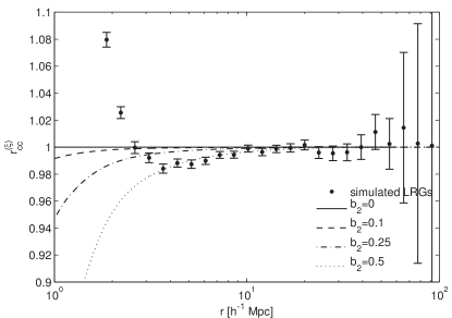
Figure 1: Correlation function cross-correlation coefficient between mock LRGs and dark matter (data points) in the simulations described in Sec. 2.1, with errors determined from the box to box variations in simulations. Lines are predictions from our model, with $r_{\mathrm{cc}}^{(\xi)}=1-(1/4)(b_{2}/b)^{2}\xi_{\text{lin}}(r)$, using a large-scale bias of $b=2.07$ (selected to match the observed large-scale $\xi_{\mathrm{g}\mathrm{g}}$ and $\xi_{\mathrm{g}\mathrm{m}}$ in the mock LRG sample) and different values of $b_{2}$, with $b_{2}=0.5$ providing the best fit to the simulated clustering and lensing observable quantities. The plot goes to larger $r$ compared to the 2d values of $R$ used in our analysis, because the measured observables at some $R$ depend on the 3d correlation functions to larger $r$.

The analysis in Baldauf et al. (2010) was focused on modeling the cross-correlation coefficient $r_{\mathrm{cc}}$, since this is the only quantity that is needed to relate the measurement of galaxy auto-correlation and galaxy-dark matter correlation to the dark matter auto-correlation. However, it is useful to analyse how well we model clustering and g-g lensing data separately with a given non-linear bias model. One reason to do so is that this allows us to choose different minimum scales ($R_{0}$) for galaxy-galaxy lensing and galaxy clustering. We expect that lensing information will be quite insensitive to the details of HOD modeling: both a satellite and a central galaxy give approximately the same g-g lensing signal for separations larger than the virial radius. So, we would expect the lensing signal to be fairly model-independent down to the virial radius. In contrast, the clustering signal will depend very sensitively on how satellite galaxies are populated within the virial radius, so the clustering signal up to at least twice the virial radius will be quite model-dependent. For example, if there are no satellites, then the clustering signal drops to almost zero within twice the virial radius, while if all the halos have one central galaxy and one satellite radially distributed as the dark matter, then the clustering signal is similar to the lensing signal. This sensitivity to how satellite galaxies populate halos suggests that we should choose a larger value of $R_{0}$ for clustering than for lensing measurements. A second reason to use larger $R_{0}$ for clustering is that the statistical errors are significantly smaller than for lensing, so the analysis of clustering data is much more sensitive to inaccuracies in the theoretical model. A third reason is that if we can model both of these functions with a few free parameters, we can use the better-measured galaxy clustering data to determine these parameters.

To do so, we require models not just for $r_{\mathrm{cc}}$, but also for scale-dependent bias, that are as realistic as possible. In order to interpret the measurements without taking ratios of noisy quantities, we must have some well-motivated way of describing the non-linear bias of the samples that we study. We consider the same local bias model of Fry & Gaztanaga (1993) as in Baldauf et al. (2010), $\delta_{\mathrm{h}}=b\delta_{\mathrm{m}}+(b_{2}/2)\delta_{\mathrm{m}}^{2}+(b_{3}/3!)\delta_{\mathrm{m}}^{3}$, which contains a local bias relation between galaxy and dark matter density up to third order and combines it with standard perturbation theory (SPT), which expands the density perturbation into a series $\delta_{\mathrm{m}}=\delta_{\mathrm{m}}^{(1)}+\delta_{\mathrm{m}}^{(2)}+...$, where $\delta_{\mathrm{m}}^{(1)}$ is the Gaussian linear theory prediction and $\delta_{\mathrm{m}}^{(n)}$ is of order $[\delta_{\mathrm{m}}^{(1)}]^{n}$, to calculate the next-to-leading order corrections to the galaxy-galaxy and galaxy-matter power spectra. The third order bias enters only through a renormalisation of the leading order bias parameter, and does not have an explicit influence on the observable correlators. At the next-to-leading order, the corrections to the galaxy-galaxy and galaxy-matter power spectra come from the auto-correlation of $\delta_{\mathrm{m}}^{2}$ and its cross-correlation with the second order density perturbation $\delta_{\mathrm{m}}^{(2)}$. In evaluating these terms, we can define (Smith et al., 2009)

$$A(k)= \int\frac{\text{d}^{3}q}{(2\pi)^{3}}F_{2}({\mn@boldsymbol{q}},{\mn@boldsymbol{k}}-{\mn@boldsymbol{q}})P(q)P(|{\mn@boldsymbol{k}}-{\mn@boldsymbol{q}}|)$$ (14)

$$B(k)= \int\frac{\text{d}^{3}q}{(2\pi)^{3}}P(q)P(|{\mn@boldsymbol{k}}-{\mn@boldsymbol{q}}|),$$ (15)

where $F_{2}$ is the SPT mode coupling kernel (see, e.g., Bernardeau et al. 2002)

$$F_{2}({\mn@boldsymbol{q}}_{1},{\mn@boldsymbol{q}}_{2})= \frac{5}{7}\alpha({\mn@boldsymbol{q}}_{1},{\mn@boldsymbol{q}}_{2})+\frac{2}{7}\beta({\mn@boldsymbol{q}}_{1},{\mn@boldsymbol{q}}_{2}),$$ (16)

with

$$\alpha({\mn@boldsymbol{q}}_{1},{\mn@boldsymbol{q}}_{2})=\frac{\left({\mn@boldsymbol{q}}_{1}+{\mn@boldsymbol{q}}_{2}\right)\cdot{\mn@boldsymbol{q}}_{1}}{q_{1}^{2}}, \!\!\!\beta({\mn@boldsymbol{q}}_{1},{\mn@boldsymbol{q}}_{2})=\frac{1}{2}\left({\mn@boldsymbol{q}}_{1}+{\mn@boldsymbol{q}_{2}}\right)^{2}\frac{{\mn@boldsymbol{q}}_{1}\cdot{\mn@boldsymbol{q}}_{2}}{q_{1}^{2}q_{2}^{2}}.$$ (17)

Upon Fourier transforming, we obtain the corresponding correlation functions, which are given by

$$\xi_{\text{gg}}(r,z)=b^{2}\xi_{\text{mm,NL}}(r,z)+2b\,b_{2}\,\xi_{A}(r,z)+\frac{1}{2}b_{2}^{2}\xi_{B}(r,z)$$ (18)

and

$$\xi_{\text{gm}}(r,z)=b\,\xi_{\text{mm,NL}}(r,z)+b_{2}\xi_{A}(r,z).$$ (19)

$\xi_{A}(r)$ and $\xi_{B}(r)$ are the Fourier transforms of $A(k)$ and $B(k)$. In principle, $\xi_{\text{mm,NL}}$ should be the correlation function corresponding to one loop perturbation theory. Taking SPT at face value, the Fourier transform is ill behaved and we replace it by the non-linear correlation function measured in the $N$-body simulations. Note that $\xi_{B}=\xi_{\text{lin}}^{2}$.

As shown in Baldauf et al. (2010), the above model can be used to predict the cross-correlation coefficient in the linear and weakly non-linear regime. It predicts $r_{\mathrm{cc}}$ to be unity on large scales and to drop below unity as one goes to smaller scales, with explicit functional form given by $r_{\mathrm{cc}}^{(\xi)}=1-(1/4)(b_{2}/b)^{2}\xi_{\text{lin}}(r)$. We know this model to be imperfect in the sense that other non-linear bias parameters at a quadratic and cubic level may be needed to properly model the data (Chan et al. 2012; Baldauf et al. 2012), but these higher order parameters may not be that different in terms of their effect on the scale dependence of the statistics we study here, so we group them into a single parameter $b_{2}$ for the purpose of this paper.

As seen in Fig. 1, this model (with parameters chosen to match mock LRG catalogues, and in particular, best-fitting $b=2.07$ and $b_{2}=0.5$) describes the correlation coefficient down to $3h^{-1}$Mpc, below which physics from within the virial radius begins to affect the results. As argued above, we expect that these effects are more significant for the auto-correlation than for the cross-correlation. We must choose the minimum scale at which we can still adopt this model. Our method for doing so will be described in Sec. 2.4; it is based on carrying out our analysis on simulated data, and checking that we can recover the true cosmology in the simulations. Before we can do so, we next describe how we model the observable quantities in real and simulated data, $\Upsilon_{\mathrm{g}\mathrm{g}}$ and $\Upsilon_{\mathrm{g}\mathrm{m}}$.

2.3 Modeling the observables

Our approach is to use Eqs. (18) and (19) to model the two observables. The data are used to constrain linear $b$, quadratic bias $b_{2}$, and the dark matter power spectrum times the matter density, as in Eq. (11). This is the full, non-linear matter power spectrum, as shown in Baldauf et al. (2010). We will use Monte Carlo Markov Chain (MCMC) methods, in which the data are compared to the model, hence for each set of cosmological parameters we must compute the fully non-linear dark matter power spectrum.

2.3.1 Matter power spectrum

We obtain the estimated linear $\xi_{\mathrm{m}\mathrm{m}}(r)$ by specifying the cosmological parameters using the camb linear gravity solver (Lewis et al., 2000), which is part of the cosmomc package that we use for the estimation of the cosmological parameters (Lewis & Bridle, 2002). We increase the accuracy of the solver, by setting accuracy_level=1.5, and checked that increasing accuracy_level does not change our results. The correlation functions $\xi_{\mathrm{m}\mathrm{m}}(r)$ are calculated at the effective redshifts of the three galaxy samples, given in Table 2.

To obtain a precise prediction for the non-linear matter power spectrum as a function of cosmological parameters, we are unable to use a standardized and publicly available emulator such as the one presented by Lawrence et al. (2010) for two reasons. First, we wish to explore variations of the Hubble parameter, $H_{0}$, which cannot be independently varied using that emulator. Second, the emulator only provides predictions for the power spectrum to a maximum wavenumber of $k=1$ $h/$Mpc, but power at higher $k$ is important when computing the matter power spectrum at our minimum scale of $R=2h^{-1}$Mpc to the required precision.

Thus, given the need to compute the non-linear power spectrum for arbitrary cosmological parameters ${\mn@boldsymbol{\theta}}$ that differ from our fiducial ones (${\mn@boldsymbol{\theta}_{0}}$), there are several possible approaches that we could take (given our simulations that are on a grid of cosmological parameters). The change in cosmological parameters affects the non-linear power spectrum in two ways: first, via the change in the linear power spectrum; and second, via the change in non-linearity corrections. Since the first effect is dominant, we account for it accurately using analytic calculations of the linear matter power spectrum, only interpolating on our simulation grid to account for the second (much smaller) effect. If we relate the non-linear and linear correlation functions via

$$\xi_{\mathrm{nl}}(r|{\mn@boldsymbol{\theta}})=\xi_{\mathrm{lin}}(r|{\mn@boldsymbol{\theta}})\frac{\xi_{\mathrm{nl}}(r|{\mn@boldsymbol{\theta}})}{\xi_{\mathrm{lin}}(r|{\mn@boldsymbol{\theta}})}\equiv\xi_{\mathrm{lin}}(r|{\mn@boldsymbol{\theta}})\alpha(r|{\mn@boldsymbol{\theta}}),$$ (20)

then we can Taylor expand $\alpha(r)$ around our fiducial cosmological parameters,

$$\xi_{\mathrm{nl}}(r|{\mn@boldsymbol{\theta}})\!\!\!\! = \!\!\!\!\!\xi_{\mathrm{lin}}(r|{\mn@boldsymbol{\theta}})\left[\alpha(r|\mn@boldsymbol{\theta}_{0})+\sum_{i}\left.\frac{\partial\alpha(r|\mn@boldsymbol{\theta})}{\partial\theta_{i}}\right|_{\mn@boldsymbol{\theta}_{0}}\!\!\Delta\theta_{i}\right]$$ (21)

$$= \!\!\!\!\!\xi_{\mathrm{lin}}(r|{\mn@boldsymbol{\theta}})\alpha(r|\mn@boldsymbol{\theta}_{0})\left[1+\sum_{i}\left.\frac{\partial\log\alpha(r|\mn@boldsymbol{\theta})}{\partial\theta_{i}}\right|_{\mn@boldsymbol{\theta}_{0}}\!\!\Delta\theta_{i}\right]$$

where the index $i$ runs over the parameters for which we have $\xi_{\mathrm{m}\mathrm{m}}$ on a grid ($\sigma_{8}$, $n_{s}$, $\Omega_{m}$, $H_{0}$, and redshift $z$). As an example of how this works for one parameter, changing $\sigma_{8}$ mostly changes the amplitude of the correlation functions by the square of the ratio of two values of $\sigma_{8}$ under consideration and this change is propagated exactly. Only the second-order change in the shape of the non-linear corrections is Taylor-expanded.

Our fiducial model has $\Omega_{m}=0.25$, $\sigma_{8}=0.8$, $n_{s}=1.0$, $h=0.7$, and $z=0.23$; we have 8 simulations of this cosmology. To obtain the derivatives of non-linear corrections with respect to cosmological parameters (needed in Eq. 21), we use further models with $\Omega_{m}=(0.2,0.3)$, $\sigma_{8}=(0.7,0.9)$, $n_{s}=(0.95,1.05)$, $H_{0}=(65,75)$ km s^-1 Mpc^-1, and 7 different redshift slices between $z=0$ and $z=0.51$. Non-linear correlation functions for these models are obtained from $N$-body simulations (Smith, 2009). For each non-fiducial model, all parameters but one are kept at the fiducial value. For the parameters for which we have two simulations bracketing the fiducial value ($\Omega_{m}$, $\sigma_{8}$, $z$, $H_{0}$), we use different derivatives depending on whether the corresponding value for the target model is above or below the fiducial value. We opted to do this rather than calculating the second derivative to avoid numerical errors blowing up when the quadratic term becomes dominant. By construction, such modelling exactly reproduces the non-linear matter correlation function for models for which we have simulations.

2.3.2 Massive neutrinos

We would also like to place constraints on massive neutrinos, which requires some additional corrections to the formalism in Sec. 2.3.1. We parametrise the neutrino mass effect as the sum of masses for the three neutrino families, $\sum m_{\nu}$, and include three different ways that they affect the matter power spectrum. First, lensing is sensitive to the total gravitational potential, which includes a contribution from massive neutrinos. This requires us to use the Poisson equation to relate potential to density perturbations, the latter of which must include the neutrino contribution ($\delta\rho=\rho_{\rm cdm}\delta_{\rm cdm}+\rho_{\rm b}\delta_{\rm b}+\rho_{\nu}\delta_{\nu}$, where cdm, b and $\nu$ subscripts denote cold dark matter, baryons and neutrinos, respectively). For $\sum m_{\nu}=0.15$ eV, $f_{\nu}=\rho_{\nu}/(\rho_{\rm cdm}+\rho_{\rm b})=0.6$ per cent, and since neutrino perturbations go from $\delta_{\nu}=\delta_{\rm cdm}$ on large scales to $\delta_{\nu}=0$ on small scales, this effect suppresses the weak lensing power spectrum on small scales by 1.2 per cent.

The second effect is the usual suppression of matter fluctuations due to the fact that neutrino fluctuations are suppressed on small scales, which in turn leads to a suppressed growth of cold dark matter and baryon fluctuations. For $\sum m_{\nu}=0.15$ eV, this effect leads to a 8 per cent suppression of the matter power spectrum. The two effects combined thus lead to 9.2 per cent suppression.

The third effect is the non-linear evolution correction, which further enhances this effect. For $k<0.1h/\mathrm{Mpc}$ the effect of neutrinos on the matter power spectrum in the linear regime can be described as a reduction of the amplitude and a red tilt (Bird et al. 2012). For $\sum m_{\nu}=0.15$ eV, this is a 4 per cent reduction in $\sigma_{8}$ and -0.01 reduction in $n_{s}$. Most of the mode coupling responsible for the non-linear effects comes from the long wavelength modes with $k<0.1h/\mathrm{Mpc}$, so it is reasonable to assume that the non-linear effects can be described with a change of amplitude and slope, scaling linearly with $\sum m_{\nu}$,

$$n_{s,\rm{eff}}=n_{s}-0.01\frac{\sum m_{\nu}}{0.15~{}\rm eV}.$$ (22)

The change of amplitude, $\sigma_{8,\rm{eff}}=\sigma_{8}-0.04[\sum m_{\nu}/(0.15~{}\rm eV)]$, is already automatically included since we compute $\sigma_{8}$ for a given cosmological model using its power spectrum. The spectral index seen by the non-linear correction is not the actual one, but the effective one given by the above equation. This is justified by noting that the most important quantities that determine the shape of the non-linear correction are the amplitude and slope of the power spectrum at a relevant pivot scale ($k\sim 0.1h/\mathrm{Mpc}$ in our case). Since the change in amplitude is already included in the change of $\sigma_{8}$, we just approximate the change in the slope of the linear power spectrum at the pivot point for $m_{\nu}$ as the change in the spectral index.

To test this procedure, we compare the resulting non-linear to linear power spectrum correction for massive neutrinos to the full simulations presented in Bird et al. (2012). For example, for the total neutrino mass of $\sum m_{\nu}=0.15$ eV, we find that the reduced linear amplitude of the power spectrum at the pivot point is 8 per cent, corresponding to a 4 per cent change in $\sigma_{8}$. This leads to a further non-linear suppression of power, up to 3 per cent at $k\sim 1h/\mathrm{Mpc}$. In addition, the effective slope is reduced by 0.01 at the pivot point. This means that for massive neutrinos there is more power on large scales than in the zero mass case, relative to the pivot point. As a result, there is more mode-mode coupling which increases the small scale non-linear power, countering the effect from the reduced linear amplitude. The net effect is that the non-linear correction peaks at $k\sim 1h/\mathrm{Mpc}$, but this quickly reverses sign above $2$$h/\mathrm{Mpc}$. The overall effect is in a good agreement with the results of the full simulations of massive neutrinos in Bird et al. (2012). This suggests that we can parametrise the non-linear effect of massive neutrinos simply with the change in the effective amplitude and slope of the linear power spectrum.

To summarise the neutrino mass effects: at $k\sim 0.5h/\mathrm{Mpc}$, which is the peak of the contribution to $\Upsilon$ at $R=5h^{-1}\mathrm{Mpc}$ and $R_{0}=3h^{-1}\mathrm{Mpc}$ (Fig. 2 of Baldauf et al. 2010) and where we expect to have the most stringent constraints from our data set, we expect about 10 per cent suppression of the power for $\sum m_{\nu}=0.15$ eV, relative to the zero mass case.

2.3.3 Cosmology corrections

When estimating the signal from the data, we assume a cosmological model in order to convert angular distances $\Delta\theta$, shears $\gamma_{t}$, and redshift-space separations $\Delta z$ to transverse separation $R$, lensing surface density contrast $\Delta\Sigma$, and line-of-sight separation $\Pi$. Thus, for the model predictions for any other cosmology than the fiducial cosmology, we should in principle include a factor in both the transverse separation and the amplitude of the measured signals to account for the fact that the wrong cosmology was used to do these conversions from observed to physical separations. However, for the highest redshift sample (for which this is most important), the size of the corrections is typically $\lesssim 1$ per cent for the range of allowed cosmological models. The correction is even smaller for the other samples, therefore it is well within the statistical error for this analysis, and we do not include it.

2.3.4 Combining the model ingredients

Finally, we need to combine these model ingredients to obtain $\xi_{\mathrm{g}\mathrm{m}}(r)$ and $\xi_{\mathrm{g}\mathrm{g}}(r)$. We do so by using the non-linear matter power spectrum for a given cosmology from Sec. 2.3.1 along with Eqs. 18 and 19.

The results are then integrated to obtain the projected statistics that we use in reality. For the lensing signals, we integrate the correlation function along the line-of-sight to $\pm 140$$h^{-1}\mathrm{Mpc}$, consistent with the fact that the lensing window is extremely broad. We do not include that window directly, but as shown in Baldauf et al. (2010) fig. 9, its effects are very small on the scales we use for science, and can be corrected for in a single factor that includes the clustering line-of-sight integration length, redshift-space distortions (RSD), and the lensing window. Given that this correction factor is $\sim 3$ per cent at 60$h^{-1}\mathrm{Mpc}$, much smaller than the observational errors, and $\sim 1$ per cent below 30$h^{-1}\mathrm{Mpc}$, we neglect this correction. For clustering, we integrate along the line-of-sight to $\pm 60$$h^{-1}\mathrm{Mpc}$, consistent with the observational measurements. Finally, for both the lensing and clustering we use the projected surface densities to obtain $\Upsilon$.

Because we have some uncertainty in the calibration of the lensing signal due to several systematic errors (Sec. 4.2.1), we include a nuisance calibration bias parameter for the g-g lensing, which is assumed to have a mean zero and a Gaussian width of $(4,4$, and $5)$ per cent for the 3 samples. The calibration bias is assumed to be the same at all radii and for all samples - i.e., if the calibration bias is 4 per cent for Main-L5 then it is 4 and 5 per cent for LRG and LRG-highz. This treatment is appropriate since the lensing calibration biases originate from the same sources for each sample, and improper estimation and removal of those biases would affect all samples nearly equally.

2.4 Choice of $R_{0}$

Baldauf et al. (2010) considered relatively large values of $R_{0}$ such as $3$ and $5$$h^{-1}\mathrm{Mpc}$. Use of a large value of $R_{0}$ is advantageous from the perspective of systematic error, because it means that we are less sensitive to several effects that tend to be worse at small scales: cross-correlation coefficient deviations from $1$, deviations from our model for non-linear bias, and observational issues such as intrinsic alignments.

However, use of larger $R_{0}$ will necessarily remove more of the measured signal, resulting in a noisier measurement. We therefore revisit the choice of $R_{0}$ in order to achieve a fair compromise between statistical and systematic error. Moreover, unlike in Baldauf et al. (2010), we permit different $R_{0}$ for the galaxy-galaxy lensing and the galaxy clustering, which is possible in the case that we explicitly model the signals (i.e., using different $R_{0}$ means that results cannot be obtained by taking ratios of the two signals). The galaxy clustering signal is more sensitive than the galaxy-galaxy lensing to the fidelity of the non-linear bias model (because it has higher signal-to-noise), so it might require a higher $R_{0}$ to avoid systematic errors.

We choose values of $R_{0}$ for the two measurements based on modeling the simulated LRG sample using the same machinery that we use to model the data (but without adding lensing shape noise, so that deviations from the real cosmology in the simulations are due to a real analysis bias). We decided to use $R_{0}=2$ and 4$h^{-1}\mathrm{Mpc}$ for galaxy-galaxy lensing and galaxy clustering, respectively, since we find this choice still gives a small systematic error compared to the statistical error, as shown in Appendix A. The corresponding plots of $\Upsilon$ are shown in Fig. 2, and we see that the simulated data and the best model agree reasonably well both for galaxy-galaxy lensing and galaxy clustering, with $b_{2}=0.25$ working acceptably. Note that $b_{2}=0.5$ best describes the cross-correlation coefficient for $\xi$, as seen in Fig. 1. In fact for the simulated data, values in the range from $b_{2}=0.25$ and $0.5$ are able to describe the data within the limits of our errorbars. A study carried out independently from this work (Cacciato et al., 2012b) has also studied the value of $R_{0}$ for which we can safely achieve $r_{\mathrm{cc}}\sim 1$ at all $R>R_{0}$, in the context of a more general HOD model. They identify $3$$h^{-1}\mathrm{Mpc}$ as a reasonable choice of $R_{0}$ (assuming the same $R_{0}$ is used for both measurements), nicely consistent with our findings.

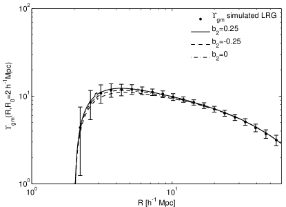
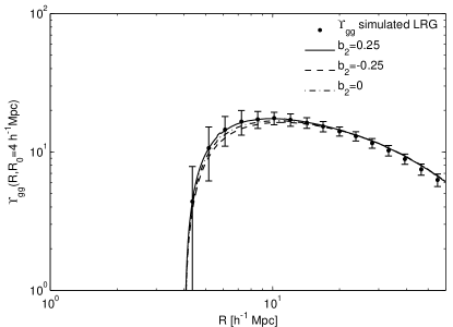
Figure 2: Top: $\Upsilon_{\text{gm}}$ for mock LRGs and the model predictions. Bottom: $\Upsilon_{\text{gg}}$ for mock LRGs and the model predictions.

2.5 Parameter values and constraints

Our convention is to quote parameter values based on the median of the posterior distribution after marginalisation over all other parameters. Except where explicitly stated otherwise, we include a prior that is a function of $\sigma_{8}$, based on our calibration on simulations in Appendix A. The quoted error-bars come from using the PDF to determine the 68, 95, and 99.7 per cent confidence intervals.

3 Data

Here we describe the data used in this paper, all of which comes from the Sloan Digital Sky Survey (SDSS). The SDSS (York et al., 2000) imaged roughly $\pi$ steradians of the sky, and followed up approximately one million of the detected objects spectroscopically (Eisenstein et al., 2001; Richards et al., 2002; Strauss et al., 2002). The imaging was carried out by drift-scanning the sky in photometric conditions (Hogg et al., 2001; Ivezić et al., 2004), in five bands ($ugriz$) (Fukugita et al., 1996; Smith et al., 2002) using a specially-designed wide-field camera (Gunn et al., 1998). These imaging data were used to create the cluster and source catalogues that we use in this paper. All of the data were processed by completely automated pipelines that detect and measure photometric properties of objects, and astrometrically calibrate the data (Lupton et al., 2001; Pier et al., 2003; Tucker et al., 2006). The SDSS-I/II imaging surveys were completed with a seventh data release (Abazajian et al., 2009), though this work will rely as well on an improved data reduction pipeline that was part of the eighth data release, from SDSS-III (Aihara et al., 2011); and an improved photometric calibration (‘ubercalibration’, Padmanabhan et al., 2008).

Below we describe the samples that are used as lenses and as sources.

3.1 Main sample lenses

The first lens sample that we use for this work is the flux-limited Main galaxy sample (Strauss et al., 2002) from SDSS DR7. The nominal flux limit is $r<17.77$, when defined using Petrosian magnitudes (based on a modification of Petrosian 1976 described in Blanton et al. 2001 and Yasuda et al. 2001). In reality, the actual flux limit varies slightly across the survey area. We use the Main sample selection from the NYU Value-Added Galaxy Catalog (VAGC, Blanton et al., 2005), which includes 7966 deg² of spectroscopic coverage (though we will employ further area cuts, described below).

We select our sample using the ‘LSS sample’ DR7-2 in the VAGC, which carefully tracks the spectroscopic flux limit and completeness across the sky. The particular LSS samples that we use are ‘dr72full8’ through ‘dr72full10’, where ‘full’ samples have the following properties:

• They use all galaxies from $r>10$ to the position-dependent flux limit.

• They use areas with any level of completeness (even $<0.5$, which occurs very rarely).

• Galaxies that did not get a spectrum due to fibre-collisions are assigned a redshift using the nearest-neighbour method.

The ‘8’, ‘9’, and ‘10’ subsamples have the following properties, some of which will be subject to more cuts described below:

• Redshift $0.001<z<0.4$

• The $k$-corrections are to $z=0.1$ (kcorrect v4_1_4; Blanton & Roweis 2007).

• The distance modulus $\mu=5\log{[D_{L}/(10\mathrm{pc})]}$ is determined using $\Omega_{m}=0.3$, $\Omega_{\Lambda}=0.7$. This is formally inconsistent with the numbers used in the rest of this paper. However, this is not a significant issue here where we simply seek a reasonably volume-limited and consistent sample (particularly given the weak dependence of the distance modulus on cosmology for these redshifts).

• The luminosity evolution is assumed to have the form

  $$M(z)=M(z=0.1)-2[1-(z-0.1)](z-0.1),$$ (23)

  which is chosen to match the number counts of SDSS spectroscopic galaxies. Given the redshift limits of our sample, this correction is constrained to lie within the range $[-0.17,0.10]$.

• The absolute magnitude is defined, in terms of the Petrosian magnitude $r$ and galaxy redshift $z$, correcting for luminosity evolution, as

  $$M_{r}=r-[\mu+k_{0.1}(z)+M(z)-M(z=0.1)].$$ (24)

  Given that the luminosity evolution is such that galaxies were brighter in the past, the definition here removes that trend, connecting galaxies at one redshift to those that were suitably brighter at earlier times according to the empirically-determined evolution law in Eq. (23).

• The absolute magnitude is then required to be in the range $[-22,-21]$, $[-21,-20]$, and $[-20,-19]$ for the three samples, respectively.

The effective area of the LSS sample is 7279 deg². We then imposed some additional cuts on the area, removing regions without any source galaxies in the background or within a Tycho bright star map (Høg et al., 2000). These cuts reduce the effective area to 7131 deg².

We wish to avoid overlap with the LRG lens samples described in the upcoming subsection, so that the cross-covariance between the signals with different lens samples can be assumed to be zero. Thus, we first require $0.02<z<0.155$ (where the lower redshift cut removes galaxies for which it would be computationally prohibitive to measure correlations to 70$h^{-1}\mathrm{Mpc}$, and the upper redshift cut removes overlaps with LRGs). We then defined the three LSS samples using the notation from Mandelbaum et al. (2006a): L3 with $-19>M_{r}\geq-20$, L4 with $-20>M_{r}\geq-21$, L5 with $-21>M_{r}\geq-22$. We do not define any brighter samples because their low abundance means that there are very few galaxies in those samples after the $z<0.155$ cut.

In practise, carrying out the analysis with all three samples requires caution: if the redshift ranges overlap (as naturally occurs for a flux-limited sample), then for scales above $R\sim 8h^{-1}$Mpc, we find that the clustering and lensing signals exhibit high cross-correlations between the samples – typically $80$ per cent – because they trace similar large-scale structures. When limiting to volume-limited samples that do not overlap, the statistical power of L3 and L4 becomes relatively low on cosmological scales. In addition, our non-linear bias model in Sec. 2 was only tested on simulations with relatively high-mass halos ($M_{\mathrm{vir}}\gtrsim 1\times 10^{13}h^{-1}M_{\odot}$). Given the typical halo masses for L3 and L4 in Mandelbaum et al. (2006a), we conclude that the optimal way of including the Main sample in this analysis is to use L5 only. This sample (referred to as ‘Main-L5’ in the rest of the paper) includes 69 150 galaxies, and is volume-limited for the redshift range that we use.

For computation of cosmological observables, we require a set of random points that are distributed in the same way as the lens sample. We therefore use the sets of random points distributed for this sample in the VAGC LSS sample; this includes a proper redshift distribution that depends on the position-dependent flux limit at each point. For weighting, we use the inverse of the ‘sector completeness’ defining the redshift success rate. The sector completeness for this sample has a median value of 0.972; 95 per cent of the galaxies have completeness above 0.924.

The area coverage of the lens sample (7131 deg², or $f_{\mathrm{sky}}=0.17$) is shown in Fig. 3. This coverage is strictly a subsample of the source catalogue from Reyes et al. (2012) that we describe in Sec. 3.3.

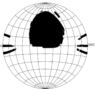
Figure 3: Area coverage of the lens samples used in this paper.

The redshift distribution $\mathrm{d}p/\mathrm{d}z$ and the comoving number density $\bar{n}$ are shown for the Main L5 sample, and for the other samples described in subsequent subsections, in Fig. 4. For the Main-L5 sample, the comoving number density is $\sim 10^{-3}(h/\text{Mpc})^{3}$.

The properties of this sample (and those introduced in subsequent sections) are summarised in Table 2. For the lensing, the effective redshift $z_{\mathrm{eff,gm}}$ is determined not just by the lens redshift distribution, but also by geometric factors related to the relation between lens and source redshifts that come into the weighting scheme we use for estimating the signals (Sec. 4):

$$z_{\mathrm{eff,gm}}=\frac{\sum_{ls}w_{ls}z_{l}}{\sum_{ls}w_{ls}}$$ (25)

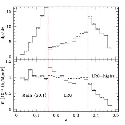
Figure 4: Top: Redshift distribution $\mathrm{d}p/\mathrm{d}z$ for the three lens samples used in this work, as labeled on the plot. The solid and dashed lines show the unweighted and weighted histograms, respectively. Bottom: Comoving number density $\bar{n}$, in units of $10^{-4}(h/\text{Mpc})^{3}$ (multiplied by $0.1$ for Main-L5 for easier viewing). The dotted vertical lines show the delineation between the different lens samples.

Sample	$N_{\mathrm{gal}}$	$z$ range	$\langle z\rangle$	$z_{\mathrm{eff,gm}}$	$\bar{n}$
name					$[(h/\mathrm{Mpc})^{3}]$
Main-L5	69 150	$0.02\leq z<0.155$	$0.115$	$0.109$	$10^{-3}$
LRG	62 081	$0.16\leq z<0.36$	$0.278$	$0.257$	$10^{-4}$
LRG-highz	35 088	$0.36\leq z<0.47$	$0.407$	$0.398$	$[8-6((z-0.36)/0.11)]\times 10^{-5}$

Table 2: Properties of the lens samples described in Sec. 3. For each sample, we show the redshift range, the mean redshifts, the effective redshift for the lensing as in Eq. 25, and the number density.

3.2 LRG sample lenses

We also define two lens samples consisting of Luminous Red Galaxies, or LRGs (Eisenstein et al., 2001). These galaxies have been used for numerous cosmology analyses with SDSS, most notably the detection of Baryon Acoustic Oscillations (BAO), which is enabled by the high galaxy bias of $\sim 2$ and the large volume probed by this sample, $\sim 0.65(h^{-1}\text{Gpc})^{3}$.

For selection of Luminous Red Galaxies, we follow the methodology of Kazin et al. (2010), which also starts from the NYU VAGC LSS sample described in the previous subsection. In this case, only regions with completeness $\geq 0.6$ are included; this definition is inconsistent with that used for Main-L5, but in practise, the discrepancy only affects 13 deg², or 0.2 per cent of the area. Our selection is otherwise identical to that from Kazin et al. (2010), with the exception of area cuts to restrict to the footprint of the source catalogue, eliminating 8 per cent of the LRGs.

Rest-frame absolute magnitudes in the $g$ band are calculated starting from the $r$ band extinction-corrected apparent Petrosian magnitude. The distance modulus assumes $\Omega_{m}=0.25$, $\Omega_{\Lambda}=0.75$. $k$-corrections and evolution corrections from Eisenstein et al. (2001) are used to convert $r$ to $M_{g}$.

Kazin et al. (2010) have a well-defined procedure for calculating weights, completeness factors, dealing with fibre collisions, and distributing random points. In brief, they begin with a calculation of sector completeness to account for all sources of incompleteness except for fibre collisions (i.e., this calculation accounts for galaxies that were allocated fibres and did not get a spectrum). This completeness is used when distributing random points in the survey area; in any given region, they are diluted according to that region’s sector completeness. To deal with the $\sim 2$ per cent of LRG targets that were not allocated fibres due to fibre collisions, a special weight is assigned; e.g., in a group of 3 LRGs of which only 2 were allocated a fibre, those two would each get a weight of $1.5$. The random points – of which there are fifteen times as many as real points – are assigned a random redshift drawn from the $p(z)$ of the real LRGs.

We define two redshift samples, which we call ‘LRG’ ($0.16\leq z<0.36$) and ‘LRG-highz’ ($0.36\leq z<0.47$). In both cases, the absolute magnitude limits are $-23.2<M_{g}<-21.2$; the former is approximately volume-limited, whereas the latter is flux-limited but relatively narrow (see Fig. 4). In the first case, we adopt a radial weighting scheme that reduces the impact of large-scale structure fluctuations on the redshift histogram. This scheme is taken directly from Kazin et al. (2010) appendix A2, is optimized for BAO studies, and does not significantly change the results, but we use it directly in order to enable a comparison between our results and other large-scale structure measurements with LRGs. In short, they bin the redshift histogram into bins of width $\Delta z=0.015$, and define a smooth $n(z)$ by doing a spline fit to that histogram. Then the radial weight is defined as $1/(1+n(z)P_{\rm fid})$ where $P_{\rm fid}=4\times 10^{4}(h/\mathrm{Mpc})^{3}$. Thus, for the LRG sample, the weights used for real points are

$$w_{\mathrm{LRG}}=\left[\frac{\text{fibre collision weight}}{\text{completeness}}\right]\left[\frac{1}{1+n(z)P_{\rm fid}}\right]$$ (26)

and for random points, the same but without any fibre collision weights. For the LRG-highz sample, we use

$$w_{\mathrm{LRG-highz}}=\frac{\text{fibre collision weight}}{\text{completeness}}.$$ (27)

In this case, since the $n(z)$ is a stronger function of redshift, it is not clear that it makes sense to include it in the weighting, and particularly not in a lensing analysis where the source density is dropping rapidly with redshift.

Once we include the redshift-dependent weighting, the LRG sample has a comoving number density that is nearly constant at $10^{-4}(h/\text{Mpc})^{3}$, a factor of ten smaller than for Main-L5. The LRG-highz sample has a comoving number density that drops with redshift because the sample is flux-limited. More details of these samples are shown in Table 2.

3.3 Sources

The catalogue of source galaxies with measured shapes used in this paper is described in Reyes et al. (2012), hereafter R12, which uses the re-Gaussianization method (Hirata & Seljak, 2003) of correcting for the effects of the point-spread function (PSF) on the observed galaxy shapes. The treatment of systematic errors is updated and improved compared to the previous SDSS source catalogue using this PSF-correction method (Mandelbaum et al., 2005), in part using tests of simulated SDSS images using real galaxies from COSMOS and real SDSS PSFs (Mandelbaum et al., 2012). To estimate source redshifts, we use photometric redshifts (photo-$z$) based on the five-band photometry from the Zurich Extragalactic Bayesian Redshift Analyzer (ZEBRA, Feldmann et al., 2006), which were characterised by Nakajima et al. (2012), hereafter N12. In particular, we use the maximum-likelihood mode for ZEBRA, and choose the best-fitting photo-$z$ after marginalizing over the SED template.

The catalogue production procedure was described in detail in R12, so we describe it only briefly here. Galaxies were selected in a 9243 deg² region, with an average number density of $1.2$ arcmin^-2. The selection was based on cuts on the imaging quality, data reduction quality, galactic extinction $A_{r}<2$ defined using the dust maps from Schlegel et al. (1998) and the extinction-to-reddening ratios from Stoughton et al. (2002), apparent magnitude (extinction-corrected $r<21.8$), photo-$z$ and template used to estimate the photo-$z$, and galaxy size compared to the PSF. The apparent magnitude cut used model magnitudes, which are defined by fitting the galaxy profile in the $r$ band to a Sérsic profile with $n=1$ (exponential) and $n=4$ (de Vaucouleurs), choosing the better of the two models, and then using that same rescaled profile to get magnitudes in all the bands. For comparing the galaxy size to that of the PSF, we use the resolution factor $R_{2}$ which is defined using the trace of the moment matrix of the PSF $T_{\mathrm{P}}$ and of the observed (PSF-convolved) galaxy image $T_{\mathrm{I}}$ as

$$R_{2}=1-\frac{T_{\mathrm{P}}}{T_{\mathrm{I}}}.$$ (28)

We require $R_{2}>1/3$ in both $r$ and $i$ bands.

The software pipeline used to create this catalogue obtains galaxy images in the $r$ and $i$ filters from the SDSS ‘atlas images’ (Stoughton et al., 2002). The basic principle of shear measurement using these images is to fit a Gaussian profile with elliptical isophotes to the image, and define the components of the ellipticity

$$(e_{+},e_{\times})=\frac{1-(b/a)^{2}}{1+(b/a)^{2}}(\cos 2\phi,\sin 2\phi),$$ (29)

where $b/a$ is the axis ratio and $\phi$ is the position angle of the major axis. The ellipticity is then an estimator for the shear,

$$(\gamma_{+},\gamma_{\times})=\frac{1}{2\cal R}\langle(e_{+},e_{\times})\rangle,$$ (30)

where ${\cal R}\approx 0.87$ is called the ‘shear responsivity’ and represents the response of the ellipticity (Eq. 29) to a small shear (Kaiser et al., 1995; Bernstein & Jarvis, 2002); ${\cal R}=1-e_{\mathrm{rms}}^{2}$. In the course of the re-Gaussianization PSF-correction method, corrections are applied to account for non-Gaussianity of both the PSF and the galaxy surface brightness profiles (Hirata & Seljak, 2003).

For this work, we do not use the entire source catalogue, only the portion overlapping the aforementioned lens samples and around the edges. Fig. 5 shows histograms of the source galaxy $r$-band apparent magnitude and photo-$z$.

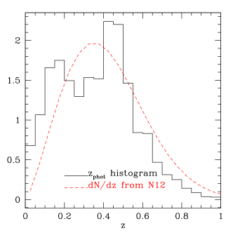
Figure 5: Histograms of source galaxy properties, derived from a random subsample of 5 per cent of the catalogue after imposing all cuts ($\sim 2\times 10^{6}$ galaxies). Top: Histogram of $r$-band extinction corrected model magnitude. Bottom: photo-$z$ histogram, and the inferred true $\mathrm{d}N/\mathrm{d}z$ from N12.

4 Observational method

In this section, we describe how we use the galaxy catalogues from Sec. 3 to measure our two observables, the galaxy-galaxy lensing and the galaxy clustering.

4.1 Galaxy-galaxy lensing

Here we describe the computation of the lensing signal. For this computation, we rely on the lens catalogues in Sections 3.1 and 3.2, and the catalogues of random lenses with the corresponding area coverage and redshift distributions. First, pairs of lenses and sources that are physically close on the sky and satisfy $z_{s}>z_{l}$ (using photo-$z$ for sources) are identified. Here, “physically close” is determined using the comoving transverse separation at the lens redshift; we require $0.02<R<32.9$$h^{-1}\mathrm{Mpc}$ for Main-L5, and $0.02<R<73.1$$h^{-1}\mathrm{Mpc}$ for the two LRG samples. These ranges are split into 37 or 41 logarithmic radial bins with $\Delta(\ln{R})=0.2$.

Lens-source pairs are assigned weights according to the error on the source shape measurement via

$$w_{ls}=\frac{1}{\Sigma_{c}^{2}(\sigma_{s}^{2}+\sigma_{SN}^{2})}$$ (31)

where $\sigma_{s}^{2}$ is the estimated shape measurement error due to pixel noise (validated in R12 by comparing measured shapes in repeat observations), and $\sigma_{SN}^{2}$, the intrinsic shape noise, was found in R12 to be $0.365$, independent of magnitude. The factor of $\Sigma_{c}^{-2}$ means that we weight by inverse variance of the expected lensing signal, thus downweighting pairs that are close in redshift because the lensing geometry is suboptimal.

Once we have computed these weights, the lensing signal in each annular bin can be computed via a summation over lens-source pairs “ls” and random lens-source pairs “rs”:

$$\Delta\Sigma(R)=\frac{\sum_{ls}w_{ls}e_{t}^{(ls)}\Sigma_{c,ls}}{2{\cal R}\sum_{rs}w_{rs}}$$ (32)

where the factor of $2{\cal R}$ arises due to our definition of ellipticity and is needed to convert tangential ellipticity $e_{t}$ to shear $\gamma_{t}$. Note that this is equivalent to the procedure in previous works such as Mandelbaum et al. (2005) of using $\sum_{ls}w_{ls}$ in the denominator and then multiplying the result by the boost factor,

$$B(R)=\frac{\sum{w_{ls}}}{\sum{w_{rs}}}.$$ (33)

The division by $\sum w_{rs}$ is necessary to account for the fact that some of our ‘sources’ are physically associated with the lens, and therefore not lensed by it.

Due to the observational strategy in SDSS, there is a tendency for the PSF to align coherently along the scan direction. This tendency gives rise to a so-called ‘systematic shear’ if the PSF correction is not perfectly efficient at removing the PSF ellipticity from the galaxy shapes, which turns out to be the case at a low level for our PSF-correction method. If a lens has a uniform distribution of sources around it, the contribution of the coherently-aligned systematic shear to the average tangential shear is zero. Thus, the systematic shear can contribute to the lensing signal primarily due to the inclusion of lenses near survey boundaries, since they lack a symmetric distribution of sources. To remove this systematic shear, we can simply subtract the lensing signal $\Delta\Sigma_{\mathrm{rand}}$ measured around random points, which will capture the geometry-dependent effect of the systematic shear. As noted by Mandelbaum et al. (2005), this correction may be imperfect in the case that the lens density fluctuates due to some effect that also modulates the systematic shear, if this modulation is not included in the random point distribution. We will return to this issue in Sec. B.5.

To compute $\Upsilon$ using Eq. (12) on our noisy, binned data, we use the following procedure. We first determine $\Delta\Sigma(R_{0})$; a discussion of how this procedure can affect results is in Mandelbaum et al. (2010). For this project, as we will show in Sec. B.1, we are helped by the fact that around $R_{0}$ there is a range of scales on which $\Delta\Sigma(R)$ is well-approximated by a power law. This situation is different from that of Mandelbaum et al. (2010), which used galaxy clusters with $R_{0}$ well within the cluster virial radius, so that the scaling of $\Delta\Sigma(R)$ was inconsistent with a power law. Thus, in this paper (unlike previous work) we can fit $\Delta\Sigma$ to a power law over a fixed range of scales, which will minimise the noise in estimation of $\Delta\Sigma(R_{0})$ that gets propagated into $\Upsilon$. We present details and tests of this procedure in Sec. B.1. After estimating $\Delta\Sigma(R_{0})$, we compute $\Upsilon$ in each radial bin using Eq. (12) directly.

For science, we only use scales above 2$h^{-1}\mathrm{Mpc}$ (4$h^{-1}\mathrm{Mpc}$) for the lensing (clustering), which results in the inclusion of 18 radial bins for LRGs and 14 for Main sample lenses (14 and 10). These bin counts take into account the fact that we exclude the nominal first radial bin above 4$h^{-1}\mathrm{Mpc}$ for the clustering, because while the bin center is above $R_{0}$, the lower edge is below $R_{0}$, and we do not attempt to model $\Upsilon$ in this rapidly-varying regime. The maximum scales of $\sim 30$ and $\sim 70$$h^{-1}\mathrm{Mpc}$ for Main-L5 and the LRG samples, respectively, were chosen based on considerations related to systematic error, which will be described in Appendix B.5. In brief, our finding is that there seem to be fluctuations of lens number densities that correlate with systematic errors in the shear for larger scales and lead to a situation where our systematic uncertainty exceeds the statistical error on the signal.

To determine errors on the lensing signal $\Delta\Sigma$ or derived quantities like $\Upsilon$, we divide the survey area into 100 equal-area jackknife subregions, each of size $\sim 71$ deg² or typical length scale $\sim 8.4$ degrees. The same division of the area into regions will be used when computing the galaxy clustering signal, so that we can also estimate the covariance between the two. This number of regions was motivated by a desire to balance two competing effects. First, we require that the number of regions be significantly larger than the number of radial bins (18), to reduce the noise in the covariance matrix (Hirata et al., 2004). Second, we require that the region size be larger than the maximum scale used for science. For the Main sample, 30$h^{-1}\mathrm{Mpc}$ (comoving) at $z=0.11$ corresponds to 5.3 degrees; for LRGs, 70$h^{-1}\mathrm{Mpc}$ at $z=0.27$ corresponds to 5.2 degrees. Thus, our typical region size is 60 per cent larger than the maximum angular scale used for science.

When computing the covariance for derived quantities such as $\Upsilon$, we estimate $\Upsilon$ for each jackknife sample to get the covariance matrix, rather than using the covariance matrix for $\Delta\Sigma$ and propagating errors.

It is well known that jackknife covariance matrices cannot be used to get cosmological constraints without some correction due to the finite level of noise (e.g., Hirata et al., 2004; Hartlap et al., 2007); this is a consequence of the fact that the inverse of a noisy, unbiased estimator of the covariance matrix is not an unbiased estimator of the inverse covariance matrix. We handle this issue by modeling the covariance matrix to eliminate noise. (While this might seem to eliminate the need to make many jackknife regions to reduce noise, as we have already done, we still need the covariance matrix to be reasonably well-determined in order to easily model it empirically.) Details of this approach will be described in Sections 5.2 and 6.2. However, we note that our results are insensitive to whether we use the noisy jackknife covariances with a correction factor (Hartlap et al., 2007) after inverting to obtain the inverse covariance, or whether we use the covariance matrices that we have modeled to reduce the noise. This finding suggests that our results are not significantly impacted by systematics related to our handling of covariance matrices.

4.2 Lensing systematic errors

A thorough treatment of systematic errors with this source catalogue is in R12. Here we include only a brief summary of the issues, along with the impact for this work.

4.2.1 Calibration biases

In Reyes et al. (2012) we considered several different types of systematic errors for which we applied corrections and estimated a total error budget. In this work we consider the same set of systematic errors, with the only change being that the lens samples are at different redshifts, thus changing the values of many of the systematic errors and their uncertainties.

To summarise briefly, our approach to estimating the systematic error budget is to consider a full list of systematic errors that affect the lensing signal calibration. We correct for our best estimate of any biases, and assign systematic errors using the following prescription: for those types of biases that are inherently connected, we assume that systematic uncertainties add linearly (e.g., two sources of 1 per cent-level uncertainty become a combined 2 per cent uncertainty); for those that are independent, we add them in quadrature (i.e. in the previous example, the combined uncertainty would be $\sqrt{2}$ per cent).

There are three calibration biases related to shear estimation that we consider to be inherently connected: errors in the correction for PSF dilution due to the PSF correction method not being perfect; noise rectification bias; and selection biases (due to our resolution cut favouring galaxies that are aligned with the shear). In R12 we described tests using realistic galaxy simulations (Mandelbaum et al., 2012) to constrain these three uncertainties together, which yielded a combined 3.5 per cent uncertainty largely independent of the lens redshift.

The other calibration biases that we consider to be independent are the impact of photo-$z$ error (as discussed thoroughly in N12); stellar contamination, which we constrain using space-based data; PSF model uncertainty; and shear responsivity errors due to incorrect estimation of the RMS galaxy ellipticity. Of these, the first is the dominant one (1, 2, and 3 per cent uncertainty for Main-L5, LRG, and LRG-highz respectively – because as shown in N12, the systematic uncertainty is larger for higher redshift samples, where cosmic variance in the calibration samples is more important). Both stellar contamination and PSF model uncertainties are $\lesssim 0.5$ per cent. Shear responsivity uncertainty is 1 per cent for all samples. Thus, the three shear biases listed previously are the dominant uncertainty for all samples; when we add up the independent effects in quadrature, we obtain a 4, 5, and 5 per cent systematic uncertainty for Main-L5, LRG, and LRG-highz, respectively.

For the purpose of simplifying the modeling, we assume that this final calibration uncertainty has a Gaussian error distribution, which may not be quite correct in detail. Moreover, since the errors were assessed in the same way for each lens sample, we assume that they are 100 per cent correlated – i.e. if the calibration is really 4 per cent too high for Main-L5, then it is 5 per cent too high for LRG and LRG-highz. We include this calibration uncertainty in the modeling of the lensing signal.

To test our understanding of the calibration biases, we present several ratio tests (Mandelbaum et al., 2005), i.e. comparisons of the signal computed using the same lens samples, but with different subsamples of the source catalogue. After we correct for our understanding of the calibration biases, we should find that the ratios of these signals are consistent with $1$ within the errors.

4.2.2 Scale-dependent systematics

Mandelbaum et al. (2010) includes a list of scale-dependent systematic errors that complicate the inference of cluster masses from the cluster lensing signal. Fortunately, many such errors are sufficiently small for galaxy-scale lenses and/or on the $>2$$h^{-1}\mathrm{Mpc}$ scales that we use for science that we can ignore them. The scale-dependent systematic errors that we do consider are intrinsic alignments of galaxy shapes (e.g., Hirata & Seljak, 2004), given that we know some of our ‘sources’ are really physically associated with the lens and therefore may tend to point towards the lens. In principle, this effect can be quite important if we have no way of removing galaxies that are physically associated with lenses from our source sample; fortunately, our photo-$z$ are sufficiently good that we are fairly successful at doing so. In Sec. B.3, we estimate the importance of this effect based on the fraction of physically-associated galaxies as a function of scale (see also Blazek et al. 2012).

The other main scale-dependent systematic error is the ‘systematic shear’ described in Sec. 4.1. While we can use the procedure described there to correct for it, we also must test the validity of that correction procedure, which we will do once we present the results in Sec. B.5. Moreover, the systematic shear is the main factor that determines the maximum scale that we use; our maximum scales of $\sim 30$ (Main-L5) and $\sim 70$$h^{-1}\mathrm{Mpc}$ (LRG, LRG-highz) are motivated by a desire to avoid a situation where the correction for systematic shear is comparable in size to the real lensing shear.

4.3 Galaxy clustering

We compute the galaxy clustering signals using the same logarithmic binning size and maximum $R$ as for the lensing, but with a minimum $R=0.3$$h^{-1}\mathrm{Mpc}$ (which provides some measurements below $R_{0}$ for estimating $w_{\mathrm{g}\mathrm{g}}(R_{0}=4)$).

The estimation of clustering signals for the lens samples relies on SDSSpix software to rapidly identify galaxy pairs within the required separation on the sky. To compute the galaxy auto-correlation $w_{\mathrm{g}\mathrm{g}}(R)$, we begin by computing the 3D galaxy correlation function $\xi_{\mathrm{g}\mathrm{g}}$ on a grid of values in $(R,\Pi)$ where $\Pi$ is the comoving line-of-sight separation with respect to the mean position of the galaxies in the pair. Our estimator for the correlation function is a generalisation of that from Landy & Szalay (1993),

$$\xi_{\mathrm{g}\mathrm{g}}(R,\Pi)=\frac{DD-2DR+RR}{RR},$$ (34)

using sums of products of weights rather than numbers of pairs of data-data, data-random, and random-random pairs. Here, the weights for a given pair come from the product of the weight for each galaxy in the pair, where the weight per galaxy is initially defined as in Sec. 3 (e.g., Eq. 26). For the LRG and LRG-highz samples, there is an additional factor in the weight, to account for the fact that the g-g lensing and galaxy clustering measurements would have different effective weights since the g-g lensing automatically includes a lensing weight factor that depends on the redshift distribution of the source galaxies. This lensing weight is a decreasing function of redshift, and we include it in the clustering analysis so that the two measurements will not have different effective amplitudes (or even shapes, since the full scale-dependent matter clustering and non-linear bias can evolve with redshift). We define this weight by taking a grid of lens redshifts starting at our minimum lens redshift and having $\Delta z=0.01$, and for each lens redshift on the grid, we use our source sample to identify lens-source pairs in the full range of $R$ used for this analysis, with $w(z)=\sum_{ls}w_{ls}$. The weight therefore includes the photometric redshift distribution of the sources, and all appropriate weight factors. In practise, it turns out that this weight is not important for Main-L5 because those galaxies are well below the bulk of the source redshift distribution and because the Main-L5 redshift distribution is rather narrow. For LRGs, it is more important, changing the effective redshift of the clustering measurement by $\Delta z=0.03$.

The projected correlation function $w_{\mathrm{g}\mathrm{g}}(R)$ is formally defined as

$$w_{\mathrm{g}\mathrm{g}}(R)=\int\xi_{\mathrm{g}\mathrm{g}}(r=\sqrt{R^{2}+\Pi^{2}})\,\mathrm{d}\Pi$$ (35)

integrated along the entire line-of-sight. In practise, we compute $w_{\mathrm{g}\mathrm{g}}(R)$ via a limited summation,

$$w_{\mathrm{g}\mathrm{g}}(R)=\Delta\Pi\sum_{i}\xi_{\mathrm{g}\mathrm{g}}(R,\Pi_{i}),$$ (36)

in $40$ bins in $\Pi$ that are linearly spaced with $\Delta\Pi=3$$h^{-1}\mathrm{Mpc}$, spanning a range $-\Pi_{\mathrm{max}}\leq\Pi\leq\Pi_{\mathrm{max}}$, for $\Pi_{\mathrm{max}}=60$$h^{-1}\mathrm{Mpc}$ (we consider the impact of this choice of $\Pi_{\mathrm{max}}$ in Sec. C).

To estimate $\Upsilon_{\mathrm{g}\mathrm{g}}(R)$, we use Eq. (2), replacing $\Sigma$ with $w_{\mathrm{g}\mathrm{g}}$, which requires an estimate of $w_{\mathrm{g}\mathrm{g}}(R_{0})$. As for the lensing signal, we identify a range of scales for which the signal is approximately a power law, and fit $w_{\mathrm{g}\mathrm{g}}$ to a power-law on those scales to estimate $w_{\mathrm{g}\mathrm{g}}(R_{0})$. Tests of this determination of $w_{\mathrm{g}\mathrm{g}}(R_{0})$ are presented in Sec. C.1. We then employ Eq. (2) to get $\Upsilon_{\mathrm{g}\mathrm{g}}$; the first term, an integral over all scales above $R_{0}$, is done via summation. For each bin, we effectively assume a constant $w$ within the bin, and we carefully account for partial bins that fall in the $R$ range of interest.

As for the lensing signal, we use the division of the lens samples into equal-area jackknife regions to compute covariance matrices, and we present the results of the jackknife covariances and modeling them to reduce the noise in Sec. 6.2.

4.4 Galaxy clustering systematic errors

There are several possible systematic errors in the calculation of the galaxy clustering statistics.

One issue is the handling of the integral in Eq. (36), with the finite line-of-sight cutoff. Naively, we can account for this in our modeling of the clustering signal by integrating the theoretical 3D correlation function to the same line-of-sight cutoff. However, as illustrated by Padmanabhan et al. (2007), this approach is uncertain at the level of tens of per cent on large scales by redshift-space distortions (RSD), and a linear treatment (Kaiser, 1987) is not likely to be adequate on these scales (e.g., Reid & White, 2011). Fortunately, as illustrated by Baldauf et al. (2010), the uncertainty induced by the redshift-space distortions is far less important for the observable that we use for science, $\Upsilon_{\mathrm{g}\mathrm{g}}$. As shown in figure 8 (right panel) in that paper, the impact of RSD and the finite line-of-sight cutoff is reduced from $\sim 30$ per cent bias on $w_{\mathrm{g}\mathrm{g}}$ to $\sim 5$ per cent bias on $\Upsilon_{\mathrm{g}\mathrm{g}}$ at the maximum scale that we use for science, and is very small below $30$$h^{-1}\mathrm{Mpc}$. We could apply a correction for this small, residual systematic error, but as described in Sec. 2.3.4, a combined correction for this effect and others (e.g., the lensing window, which goes in the opposite direction) is so small as to be negligible for our analysis.

Because $\Upsilon_{\mathrm{g}\mathrm{g}}$ is a partially compensated statistic, it is also less sensitive to large-scale density fluctuations that can shift $w_{\mathrm{g}\mathrm{g}}$ up and down. We will demonstrate the effect of this on the cosmic variance component of the errors in Sec. 6.2. The same argument is true for the integral constraint, which will lead to a constant offset in $w_{\mathrm{g}\mathrm{g}}$ which goes away when computing $\Upsilon_{\mathrm{g}\mathrm{g}}$.

There are also a question of how sample definition choices affect the measured statistics. Kazin et al. (2010) consider several such effects for $w_{\mathrm{g}\mathrm{g}}$, including the method of distributing the random points in redshift, and the way of handling fibre collisions in the weighting. Their conclusion that these issues are only important at the few per cent level at most is also applicable to our results, and thus this systematic error is subdominant to the statistical and systematic uncertainties in the lensing signal.

5 Results of lensing measurements

In this section we present the galaxy-galaxy lensing measurements (Sec. 5.1), the error estimates (Sec. 5.2). Tests for systematic errors are in Appendix B.

5.1 Observations

The lensing signals for all three samples are shown in Fig. 6. This figure shows the observable quantity, $\Delta\Sigma$, and also the quantity used for cosmological constraints, $\Upsilon_{\mathrm{g}\mathrm{m}}(R_{0}=2h^{-1}\text{Mpc})$, plotted as $R\Upsilon$ for easier viewing on a linear scale. Clearly the $S/N$ of the observable is quite high – typically $\sim 25$ averaged over all scales, using

$$\frac{S}{N}=\left({\mn@boldsymbol{x}}^{T}{\bf C}^{-1}{\mn@boldsymbol{x}}\right)^{1/2},$$ (37)

where ${\mn@boldsymbol{x}}$ is the vector of $\Delta\Sigma$ values in each radial bin and ${\bf C}$ is their covariance matrix, to account for correlations between bins. The shear is well-constrained down to a level of $\sim 5\times 10^{-5}$ (at $\sim 5$ degree angular separations), and the results are statistically consistent with previously-published ones for LRGs with $R<4$$h^{-1}\mathrm{Mpc}$ (Mandelbaum et al., 2006b). Comparison with previous Main-L5 observations is complicated by our imposition of a redshift cut $z<0.155$, and this is the first such galaxy-galaxy lensing observation for LRG-highz.

$\Upsilon_{\mathrm{g}\mathrm{m}}$ is a lower $S/N$ quantity, with total average $S/N$ of 11, 14, and 8 for Main-L5, LRG, and LRG-highz, averaged over the range of scales ($2<R<70$$h^{-1}\mathrm{Mpc}$) shown on the plot.

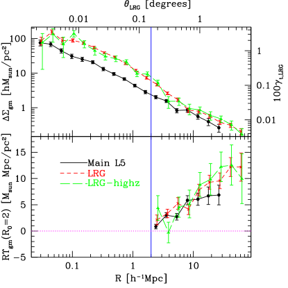
Figure 6: Top: Observed lensing signal $\Delta\Sigma_{\mathrm{g}\mathrm{m}}(R)$ for all three lens samples. The vertical line indicates the minimum scale used for cosmological constraints. The axes on the top and right indicate the angular scale $\theta$ and the tangential shear $100\gamma_{t}$ for the LRG sample. Bottom: $R\Upsilon_{\mathrm{g}\mathrm{m}}(R;R_{0}=2)$ for all three samples as labeled on the plot.

A detailed discussion of tests for systematic errors in the lensing signal is in Appendix B.

5.2 Covariance matrices

Here, we present the error estimates for the $\Upsilon_{\mathrm{g}\mathrm{m}}$ results shown above. As stated in Sec. 4.1, the noisiness of the jackknife covariance matrices requires some correction in order to get cosmological parameter estimates. Rather than modifying the procedure for using them to get confidence intervals, as in Hirata et al. (2004) or Hartlap et al. (2007), we instead model the matrices to make noiseless versions.

The process begins by modeling the diagonal terms of the covariance matrix as a function of $R$. We refer to the covariance matrix for $\Upsilon_{\mathrm{g}\mathrm{m}}$ as ${\bf C}_{\mathrm{gm}}^{(\Upsilon)}$ with elements corresponding to radial bins $i$ and $j$ of ${\bf C}_{\mathrm{gm}}^{(\Upsilon)}(R_{i},R_{j})$. Our smooth model is

$${\bf C}_{\mathrm{gm}}^{(\Upsilon)}(R_{i},R_{i})=AR^{-2}[1+(R/R_{t})^{2}],$$ (38)

with an amplitude $A$ and a turnover radius $R_{t}$. This two-parameter model is motivated as follows: on all scales, we expect sampling variance to be minimal because of the large area and the compensated nature of $\Upsilon$, so shape noise should be the dominant source of error. The shape noise variance scales like $R^{-2}$ for logarithmically spaced annular bins, and we fit for the amplitude $A$ of this term. However, as shown in Jeong et al. (2009), above some radius the shape noise fails to decrease as rapidly with $R$, in the regime where $R$ is significantly larger than the typical separation between lenses. In that case, the lens-source pairs in the annular bin include many of the same sources around nearby lenses, so the shape noise does not decrease by adding more lenses. The term in brackets in Eq. (38) represents this flattening of the errors with scale. (There will also be a corresponding increase in bin-to-bin correlations on those scales, as will shortly be apparent.)

Our approach is to model the diagonal elements of the covariance matrix by directly fitting for $(A,R_{t})$ for each lens sample using $\chi^{2}$ minimisation, doing an unweighted fit for $\log{C_{\mathrm{gm}}^{(\Upsilon)}(R_{i},R_{i})}$ as a function of $\log R$. The scale on which the term in brackets in Eq. (38) becomes important is $R_{t}=(8,31,41)$$h^{-1}\mathrm{Mpc}$ for the three samples. This trend of $R_{t}$ is unsurprising given the trends in lens number density for the three samples. In the top panel of Fig. 7, we show a comparison between the jackknife covariance diagonal terms and those from the model, for the LRG sample. As shown, the RMS level of fluctuations of the jackknife variances compared to those in the model is 12 per cent.

Next, we model the off-diagonal terms, which are also somewhat noisy. Off-diagonal terms can arise due to (a) cosmic variance (not very significant for this sample), (b) correlated shape noise due to the large $R$ compared to the separation between lenses, and (c) the fact that $\Upsilon(R)$ at some radius depends on the $\Delta\Sigma(R_{0})$, which tends to anti-correlate bins at $R\sim R_{0}$ with each other. Since there are several sources of correlations, they are not as simple to model analytically. Thus, we take a non-parametric approach, by generating the correlation matrix, i.e. ${\bf C}_{\mathrm{corr}}$, defined by

$${\bf C}_{\mathrm{corr},i,j}=\frac{{\bf C}_{\mathrm{gm}}^{(\Upsilon)}(R_{i},R_{j})}{\sqrt{{\bf C}_{\mathrm{gm}}^{(\Upsilon)}(R_{i},R_{i}){\bf C}_{\mathrm{gm}}^{(\Upsilon)}(R_{j},R_{j})}}$$ (39)

We then apply a boxcar smoothing algorithm with a length of 3 bins in radius to this matrix, to reduce the noise. The middle and bottom panels of Fig. 7 show the unsmoothed and smoothed correlation matrix for the LRG sample. As shown, the smoothing has not resulted in any significant modification of the apparent real trends, but has eliminated the majority of the noise.

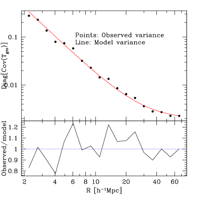
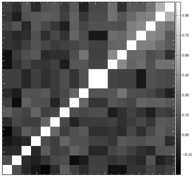
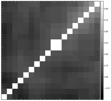
Figure 7: Top: A comparison of the jackknife covariance matrix diagonal terms for $\Upsilon_{\mathrm{g}\mathrm{m}}$ for the LRG lens sample with the model covariance matrix terms as a function of transverse separation $R$. Middle: Jackknife correlation matrix for $\Upsilon_{\mathrm{g}\mathrm{m}}$, again for LRG lenses. Bottom: Smoothed correlation matrix for $\Upsilon_{\mathrm{g}\mathrm{m}}$.

6 Results of clustering measurements

In this section we present the galaxy clustering measurements (Sec. 6.1), the error estimates (Sec. 6.2), and cross-covariance with the lensing results (Sec. 6.3). Tests for systematic errors in the clustering measurements are in Appendix C.

6.1 Observations

The clustering signals for all three samples are shown in Fig. 8. This figure shows the observable quantity, $w_{\mathrm{g}\mathrm{g}}$, and also the quantity used for cosmological constraints, $\Upsilon_{\mathrm{g}\mathrm{g}}(R_{0}=4h^{-1}\text{Mpc})$ (plotted as $R\Upsilon$ for easier viewing on a linear scale). Clearly the $S/N$ of the observable is quite high, significantly more so than for the lensing observable. $\Upsilon$ gives a total average $S/N$ of 19, 33, and 32 (Main, LRG, LRG-highz) when averaged over scales $R>4$$h^{-1}\mathrm{Mpc}$ using Eq. (37).

As discussed in Sec. 4.3, these results include a redshift-dependent weighting factor so that the effective redshift will be the same as for the galaxy-galaxy lensing measurement. Thus, they cannot be directly compared with previous measurements of LRG and LRG-highz sample clustering without checking the effect of this weighting. We find that for the LRG (LRG-highz) sample, inclusion of the lens-weighting factor has lowered the amplitude of $w_{\mathrm{g}\mathrm{g}}$ by 4 (2) per cent and increased the errors by $\sim 10$ per cent. Thus, if we had not included it, then with the same lensing signal but a higher clustering signal we would have inferred a lower $\sigma_{8}$ by 2 (1) per cent when analysing these samples, which is of similar order as other calibration factors we have considered and therefore validates our choice to include this redshift-weighting properly.

The bottom panel of Fig. 8 shows the ratio of the measured signal for the LRG sample from Zehavi et al. (2005) to our measurement without the lens-weighting, with the differences being due to our use of nearly twice as much area (7131 versus 3836 degrees²) and the different line-of-sight integration lengths ($\pm 60$ versus $\pm 80$ $h^{-1}\mathrm{Mpc}$). Even with these differences, the results agree at the 1 per cent level; the results agree to well within the naively propagated errors because the results are actually correlated to some extent, and this agreement shows that we have not done anything substantively different from the perspective of systematic errors. Additional tests for systematic errors in the clustering measurements are in Appendix C.

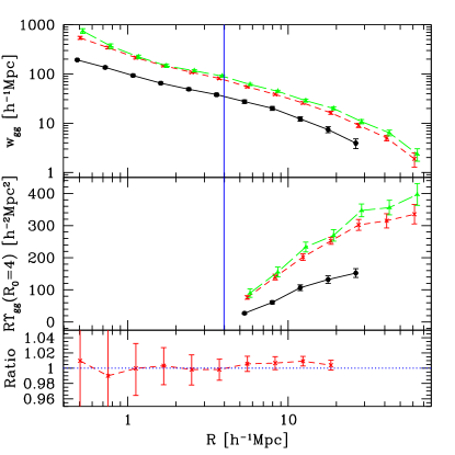
Figure 8: Top: Observed clustering signal $w_{\mathrm{g}\mathrm{g}}(R)$ for all three lens samples, including lens-weighting factors for LRG and LRG-highz. The vertical line indicates the minimum scale used for cosmological constraints. Line colours and types indicate the sample, using the same scheme as Fig. 6. Middle: $R\Upsilon_{\mathrm{g}\mathrm{g}}(R;R_{0}=4)$ for all three samples as labeled on the plot. Bottom: For the LRG sample, the ratio of $w_{\mathrm{g}\mathrm{g}}$ from Zehavi et al. (2005) to that from our work without lens-weighting, after accounting for the different radial binning.

6.2 Covariance matrix

Here, we present the error estimates for the quantities shown above, in particular, the $\Upsilon_{\mathrm{g}\mathrm{g}}$ results. We follow the approach from Sec. 5.2 of modeling the covariance matrices to reduce the noise, again showing results for the LRG sample as an example.

The process begins by modeling the diagonal terms of the covariance matrix as a function of $R$. We refer to the covariance matrix for $\Upsilon_{\mathrm{g}\mathrm{g}}$ as ${\bf C}_{\mathrm{gg}}^{(\Upsilon)}$ with elements corresponding to radial bins $i$ and $j$ of ${\bf C}_{\mathrm{gg}}^{(\Upsilon)}(R_{i},R_{j})$. Our smooth four-parameter model is

$${\bf C}_{\mathrm{gg}}^{(\Upsilon)}(R_{i},R_{i})=A_{1}R^{\alpha_{1}}+A_{2}R^{\alpha_{2}},$$ (40)

a sum of a shallower and a steeper power-law, which dominate on larger and smaller scales respectively. The choice of this functional form comes from the fact that for $\Upsilon_{\mathrm{g}\mathrm{g}}$ there is an additional noise component on small scales due to propagated uncertainty in $w_{\mathrm{g}\mathrm{g}}(R_{0})$.

We model this term by directly fitting for $(A_{1},\alpha_{1},A_{2},\alpha_{2})$ for each lens sample using $\chi^{2}$ minimisation, doing an unweighted fit for $\log{\bf C}_{\mathrm{gg}}^{(\Upsilon)}(R_{i},R_{i})$ as a function of $\log R_{i}$. In the top panel of Fig. 9, we show a comparison between the jackknife covariance diagonal terms and those from the model, for the LRG sample. As shown, the level of fluctuations of the observed variances compared to those in the model is 17 per cent (but there is a fairly extreme outlier; excluding that one noticeably decreases the estimated scatter). Smoothing the diagonal terms to reduce the influence of this outlier is important; too low a variance would result in that bin unfairly dominating the fits.

Next, we model the off-diagonal terms, which are also somewhat noisy. Off-diagonal terms can arise due to cosmic variance (not very significant for this compensated statistic $\Upsilon_{\mathrm{g}\mathrm{g}}$), but also a small contribution from the fact that $\Upsilon_{\mathrm{g}\mathrm{g}}(R)$ at some radius depends on $w_{\mathrm{g}\mathrm{g}}(R_{0})$, which tends to anti-correlate bins at $R\sim R_{0}$ with each other. Since there are several sources of these correlations, they are not as simple to model analytically. Thus, we take a non-parametric approach, by generating the correlation matrix, i.e. ${\bf C}_{\mathrm{corr}}$, defined by

$${\bf C}_{\mathrm{corr},i,j}=\frac{{\bf C}_{\mathrm{gg}}^{(\Upsilon)}(R_{i},R_{j})}{\sqrt{{\bf C}_{\mathrm{gg}}^{(\Upsilon)}(R_{i},R_{i}){\bf C}_{\mathrm{gg}}^{(\Upsilon)}(R_{j},R_{j})}}$$ (41)

We then apply a boxcar smoothing algorithm with a length of 3 bins in radius to this matrix, to reduce the noise. The middle and bottom panels of Fig. 9 show the unsmoothed and smoothed correlation matrix for the LRG sample. As shown, the smoothing has not resulted in any significant modification of the apparent real trends, but has eliminated the majority of the noise.

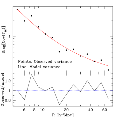
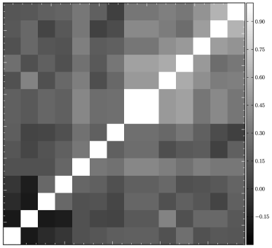
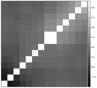
Figure 9: Top: A comparison of the jackknife covariance matrix diagonal terms for $\Upsilon_{\mathrm{g}\mathrm{g}}$ for the LRG sample, with the model covariance matrix terms as a function of transverse separation $R$. Middle: Jackknife correlation matrix for $\Upsilon_{\mathrm{g}\mathrm{g}}$ for the LRG lens sample. Bottom: Smoothed correlation matrix for $\Upsilon_{\mathrm{g}\mathrm{g}}$.

We also compare the covariance matrices for $w_{\mathrm{g}\mathrm{g}}$ and $\Upsilon_{\mathrm{g}\mathrm{g}}$, to check that they behave in the way that we expect with respect to reduced cosmic variance in the latter due to its compensated nature (Sec. 2). Fig. 10 illustrates this difference, using the LRG sample as an example. Here we have rebinned the data and covariances by a factor of two, because we do not have a smoothed version of the covariance matrix for $w_{\mathrm{g}\mathrm{g}}$. As shown, the relative error (top panel) on $\Upsilon_{\mathrm{g}\mathrm{g}}$ is larger near $R_{0}$, because $\Upsilon_{\mathrm{g}\mathrm{g}}$ is defined to be near zero there, but on large scales, $w_{\mathrm{g}\mathrm{g}}$ has a larger fractional error due to cosmic variance. We also study the correlation properties of these statistics. As shown (bottom panel), $w_{\mathrm{g}\mathrm{g}}$ exhibits larger correlations between nearby bins. This is a consequence of cosmic variance: large-scale modes can coherently shift $w_{\mathrm{g}\mathrm{g}}$ up or down, resulting in bin-to-bin correlations. In contrast, $\Upsilon_{\mathrm{g}\mathrm{g}}$ shows less significant correlation patterns.

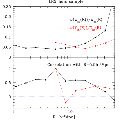
Figure 10: Error comparison for $w_{\mathrm{g}\mathrm{g}}$ (black solid lines) and $\Upsilon_{\mathrm{g}\mathrm{g}}$ (red dashed lines) for the LRG lens sample. Top: Standard deviation of these statistics (i.e., the square root of the diagonal covariance matrix elements) as a function of $R$, divided by the signal itself. Bottom: Correlation of the data at each bin in radius with the bin above $R=R_{0}$$h^{-1}\mathrm{Mpc}$.

We also compare these error properties versus the expected ones from the simulations. For the simulations, the volume has been divided into $1.5\times 1.5\times 0.3=0.67(\mathrm{Gpc}/h)^{3}$ sub-volumes, almost exactly the size of our observed volume but with slightly different geometry. There are $40$ such sub-volumes, which we use to estimate covariance matrices by comparing the signals computed in each one. This test serves as a check on the jackknife method that we carry out on the real data. We find that the scaling of $\sigma(w_{\mathrm{g}\mathrm{g}})/w_{\mathrm{g}\mathrm{g}}$ in the simulations and data is extremely similar for all scales that we use. For $\Upsilon_{\mathrm{g}\mathrm{g}}$  the same is generally true, though the errors near $R_{0}$ seem to be $\sim 20$ per cent larger in the simulations than in the data, but the opposite is true at higher $R$, with the two in agreement around 8$h^{-1}\mathrm{Mpc}$. This may be attributed to the method of determining $w_{\mathrm{g}\mathrm{g}}(R_{0})$, which differs slightly between the data analysis and simulations. Nonetheless, the comparison between errors in the simulations and in the real data is very similar, and should alleviate any concerns about the jackknife errorbars used in practise. We have also confirmed that the correlation properties for $w_{\mathrm{g}\mathrm{g}}$ and $\Upsilon_{\mathrm{g}\mathrm{g}}$ in the simulations are consistent with those we observe in the real data (bottom of Fig. 10).

6.3 Cross-covariance with lensing

Using the jackknife resampling, we are able to compute the cross-covariance between the lensing and clustering observations. Our findings are that on all scales, these correlations are consistent with zero, except possibly on the largest scales where they reach 10–15 per cent. This result is unsurprising given that the dominant source of error in our observations is the lensing shape noise. So, for the purpose of cosmological parameter constraints, we set the cross-terms between lensing and clustering in the covariance matrix to precisely zero.

For future work with surveys that are not as limited by shape noise, these covariances will be important to model accurately.

7 Cosmological parameter constraints

In this section, we present cosmological parameter constraints derived from the data that were shown in the previous section.

7.1 Constraints with these data alone

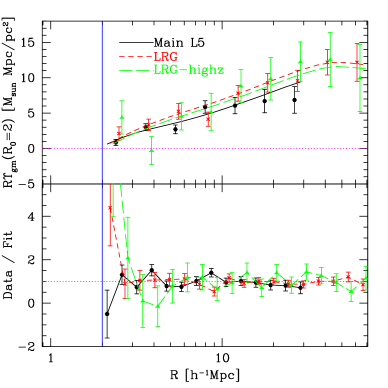
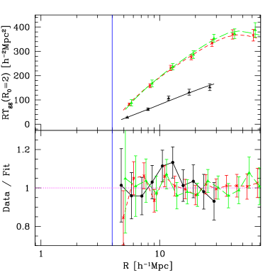
Figure 11: Top left: Observed $R\Upsilon_{\mathrm{g}\mathrm{m}}$ with best-fit signals from fits 1–3 in Table 3; for these fits, the data were fit separately for each sample. Data have been rebinned for easier viewing. Bottom left: Ratio of observed to best-fit signal from the top panel, using the original narrower binning as for the actual fit. Right: Same as left, but for clustering $R\Upsilon_{\mathrm{g}\mathrm{g}}$.

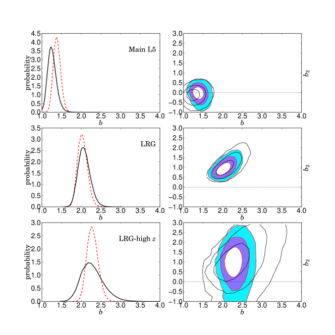
Figure 12: Best-fitting galaxy bias parameters for Main-L5 (top), LRG (middle), and LRG-highz (bottom). Left: The posterior probability distribution for the large-scale galaxy bias $b$, marginalised over other parameters including the non-linear bias parameter $b_{2}$. The solid black lines show the results for fits 1–3, fitting for each sample separately; the dashed red lines are the results from fit 4, jointly fitting all samples. Right: Contour plots for the large-scale bias $b$ versus non-linear bias parameter $b_{2}$ ($1$, $2$, and $3\sigma$). The black line contours show the results from fits 1–3, fitting for each sample separately; the coloured contours show the results from fit 4, jointly fitting all samples.

We use the standard cosmomc (Lewis & Bridle, 2002) package to make statistical inferences from our data. The package has been extended with a module that models our signals as described above and provides the likelihood that can be turned into posterior probability either alone or in conjunction with another dataset. We use the standard cosmomc parametrisation of cosmology with flat priors on the following parameters $\omega_{b}=\Omega_{b}h^{2}$ (baryon density), $\omega_{\rm cdm}$ (cold dark matter density), $\theta$ (angular diameter distance of the surface of last scattering, a proxy for Hubble’s constant), $\tau$ (optical depth to the surface of last scattering), $w$ (dark energy equation of state), $n_{s}$ (spectral index of primordial fluctuations), $A$ (amplitude of the primordial fluctuations; however, we quote our results in terms of the more commonly-used parameter $\sigma_{8}$). On top of these priors, we include a prior that is flat in $\sigma_{8}^{5}$, based on our calibration on simulations in Appendix A. We vary parameters specific to our dataset: two bias parameters for each dataset and a common calibration parameter $c$ as discussed in Sec. 2.3.4 and 4.2.1.

We start by performing the analysis using SDSS lensing and clustering data without any external priors from e.g. CMB data; this analysis is carried out both in individual redshift bins and combined. For these tests, we fix the cosmological parameters to $\Omega_{m}=0.25$, $n_{s}=0.96$, and $h=0.7$, only varying $\sigma_{8}$, the bias parameters, and the lensing calibration parameter. We do this fit for each sample separately, and for all three together (Table 3, fits 1–4).

Fit	sample	$\sigma_{8}$	$\Omega_{m}$	$b$	$b_{2}$	$b$	$b_{2}$	$b$	$b_{2}$	$\chi^{2}$	$\nu$	$\!\!\!\!\!\!\!p(>\chi^{2})$
				(L5)	(L5)	(LRG)	(LRG)	(LRG-highz)	(LRG-highz)
1	L5	$0.89^{+0.07}_{-0.08}$	0.25	$1.25\pm 0.05$	$\!\!\!-0.12\pm 0.18\!\!\!$	-	-	-	-	$29.8$	$19$	$0.06$
2	LRG	$0.79\pm 0.06$	0.25	-	-	$2.07\pm 0.05$	$\!\!\!0.98^{+0.28}_{-0.24}\!\!\!$	-	-	$19.3$	$27$	$0.86$
3	LRG-highz	$0.81\pm 0.10$	0.25	-	-	-	-	$2.26\pm 0.06$	$\!\!\!0.94^{+0.66}_{-0.54}\!\!\!$	$20.5$	$27$	$0.81$
4	All	$0.80\pm 0.05$	0.25	$1.38\pm 0.05$	$\!\!\!-0.02\pm 0.20\!\!\!$	$2.03\pm 0.05$	$\!\!\!0.94^{+0.24}_{-0.20}\!\!\!$	$2.28\pm 0.06$	$\!\!\!1.00^{+0.46}_{-0.50}\!\!\!$	$71.3$	$77$	$0.66$
5	All	$0.76\pm 0.08$	$\!\!\!\!\!\!0.269^{+0.038}_{-0.034}\!\!\!\!$	$1.46\pm 0.06$	$\!\!\!-0.06\pm 0.26\!\!\!$	$2.15\pm 0.07$	$\!\!\!0.96^{+0.36}_{-0.26}\!\!\!$	$2.44\pm 0.11$	$\!\!\!0.84^{+0.58}_{-0.64}\!\!\!$	$71.6$	$76$	$0.63$

Table 3: Fits for cosmological parameters described in Sec. 7.1. In each case, parameters that are fixed to a single value are in bold; those that are fit are shown with 68 per cent confidence limits after marginalising over all other fitted parameters.

With these fits, we can do a basic sanity test for consistency between samples. In Fig. 11 we show the data with the best-fitting signals. The model appears to fit the data quite well, without any signs of systematic tension, consistent with the reasonable $\chi^{2}$ and $p$-values in Table 3.

Fig. 12 shows the posterior distributions for the bias parameters for each sample; we show the results from fits 1–3 (fitting for the samples separately) and 4 (fitting all together). Fig. 13 shows the 1D posterior distributions for $\sigma_{8}$ for each sample separately and the combined result (fits 1–4), in all cases marginalised over the bias parameters. The corresponding limits on $\sigma_{8}$ when using all samples together (as in Table 3, fit 4) are $0.80\pm 0.05$ (68 per cent confidence level, stat. $+$ sys.). Figures 11, 12, and 13 demonstrate clearly that there is no statistically significant tension between cosmological parameter constraints from the different samples.

The results in Fig. 12 suggest that for LRG and LRG-highz, we detect non-linear bias at the $>3\sigma$ and $\sim 1.5\sigma$ levels, respectively (the results in Table 3 are deceptive; they suggest less significant detections, because the errorbars are quite non-Gaussian). The non-detection for L5 does not mean we find that the bias is linear on all scales, only above $\sim 4$$h^{-1}\mathrm{Mpc}$. Quantitatively, we find a $\Delta\chi^{2}$ for the best-fit model with $b_{2}$ free versus that with $b_{2}=0$ (linear bias only) of $(0.2,32,4.5)$ for Main-L5, LRG, and LRG-highz, respectively. That number for Main-L5 confirms the non-detection of non-linear bias, but the $\Delta\chi^{2}$ for LRG suggests a $>3\sigma$ detection of non-linear bias, with a marginal detection for LRG-highz. As expected, the best-fit model with $b_{2}=0$ has higher $\sigma_{8}=0.85$, $0.83$ for LRG and LRG-highz, to accommodate the increased clustering below 10$h^{-1}\mathrm{Mpc}$ due to non-linear bias. Note that the hierarchy of bias values for these samples roughly mirrors the trends previously detected for galaxy bias as a function of luminosity determined in SDSS using relative bias measurements, for example by Swanson et al. (2008). Furthermore, the LRG linear and quadratic biases are consistent with values that were previously measured using a combination of the two- and three-point correlation functions (Marín, 2011). While the value of $b_{2}$ for the LRG sample is roughly $2\sigma$ above the value that describes the simulated sample in Fig 1, this may simply reflect slightly stronger clustering on small scales, which can result from even slightly larger satellite fractions.

As described in Sec. 2.3.4, we have included an arbitrary galaxy-galaxy lensing signal calibration uncertainty with a Gaussian standard deviation of $(0.04,0.04,0.05)$ for the three samples, assuming the calibration is perfectly correlated between them. Given this prior, we find that the best fit is obtained with a calibration that is $0.1\sigma$ from the expected value (this decrease in the signal is illustrated in Fig. 11 via an increase of the theoretical model). If we instead fix the lensing calibration without allowing any freedom, the best-fit $\sigma_{8}$ changes by an amount that is well below our quoted error, and the errors become smaller by 20 per cent. These findings suggest that systematic uncertainty due to uncertain lensing calibration is not completely negligible, but does not dominate our error budget.

We have also carried out these fits with the off-diagonal elements of the covariance matrix set to zero for both lensing and clustering for all samples, in order to test how sensitive we are to the treatment of off-diagonal elements. We find that the best-fitting $\sigma_{8}$ changes by $0.01$ ($0.2\sigma$), and the size of the error regions becomes smaller by 15 per cent. Thus, our results are relatively stable to inclusion of correlations between radial bins.

As an empirical test of the $\sigma_{8}^{5}$ prior that was justified using simulated data in Appendix A, we confirm that when we remove the $\sigma_{8}^{5}$ prior for fit 4, $\sigma_{8}$ for the most likely point in the full fit parameter space does not correspond to that of the median of the posterior distribution after marginalizing over nuisance parameters. The sign of the difference is the same of that in the simulated data in the Appendix; the magnitude of the difference is slightly larger than that in the simulations, but the effects are consistent in the simulations and real data once we take into account the far larger noise in the real data. Thus, there is no indication from the data that the assumptions behind our $\sigma_{8}^{5}$ prior are incorrect, so we use this prior for all fits that include the SDSS lensing and clustering data.

Next, we have allowed the matter density $\Omega_{m}$ to vary (fit 5 in Table 3, using all three samples together). In this case, there is a classic degeneracy between $\sigma_{8}$ and $\Omega_{m}$ in the lensing data, with higher $\sigma_{8}$ requiring a lower $\Omega_{m}$ to fit the data. Because of this degeneracy, the allowed range of $\sigma_{8}$ becomes broader, $\sigma_{8}=0.76\pm 0.08$ when marginalised over $\Omega_{m}$, the bias parameters, and the lensing calibration (still a 10 per cent constraint on $\sigma_{8}$ even with this degeneracy). When marginalising over $\sigma_{8}$, we can constrain $\Omega_{m}=0.269^{+0.038}_{-0.034}$. The resulting 2D contour plot for these two parameters is shown in Fig. 14. The best-constrained parameter combination, which is a better illustration of our overall $S/N$, is $\sigma_{8}(\Omega_{m}/0.25)^{0.57}=0.80\pm 0.05$ ($1\sigma$, stat. $+$ sys.), representing a 6 per cent uncertainty in the amplitude of matter fluctuations. We do not show the best-fitting signal for this case, because it differs very little from that shown in Fig. 11.

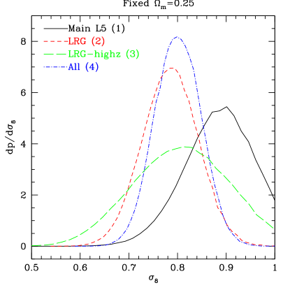
Figure 13: Posterior distribution for $\sigma_{8}$ marginalised over all other fit parameters, for fits 1–4 ($\Omega_{m}$ fixed).

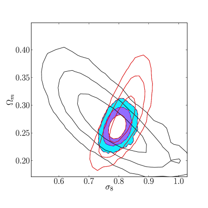
Figure 14: Open black lines show the contours in the $\sigma_{8}$ vs. $\Omega_{m}$ plane (fit 5) for our dataset, marginalising over all linear and non-linear bias parameters and lensing calibration. The contours that are shown are $1$, $2$, and $3\sigma$. The nearly orthogonal open red contours are for WMAP7 (also fitting for $n_{s}$, $H_{0}$, and other parameters in flat $\Lambda$CDM as in Sec. 7.2), and the filled contours are for WMAP7 combined with our data.

7.2 Combination with other data

We combine these data with WMAP7 CMB results (Komatsu et al., 2011), anticipating significant benefit from a tight prior on the amplitude of matter fluctuations at early times. For the first combined fit, we vary $(A,\omega_{dm},\omega_{b},\theta,\tau,n_{s})$ (see definitions at start of Sec. 7.1), the six bias parameters for the three galaxy samples, and the lensing calibration with its $(4,5,5)$ per cent Gaussian prior – with fixed $w_{\mathrm{de}}=-1$ and $\Omega_{k}=0$. We include lensing of the CMB and marginalise over an SZ template as in Komatsu et al. (2011). All results in this section that use our data include our $\sigma_{8}^{5}$ prior from Appendix A, but that prior was not included for the analyses that use WMAP7 data alone.

Fig. 15 shows 2D parameter contours with WMAP7 alone and combined with these data (the $\Omega_{m}$ vs. $\sigma_{8}$ contour was already shown in Fig. 14). We can see that since the degeneracy direction for $\sigma_{8}$ vs. $\Omega_{m}$ for the CMB data is orthogonal to that for lensing data (Fig. 14), adding our data to the WMAP7 data roughly halves the size of the allowed regions in parameter space. However, the top panel of Fig. 15 shows that the constraints on $n_{s}$ are, unsurprisingly, set exclusively by the WMAP7 data. The bottom panel shows that we also provide additional constraining power on $H_{0}$, through the stronger constraint on $\Omega_{m}$ (and the fact that CMB constrains a different parameter combination, $\Omega_{m}h^{2}$). The resulting 1D probability distributions for $(n_{s},\sigma_{8},\Omega_{m},H_{0})$, marginalised over other parameters, are shown in Fig. 16.

Table 4 gives best-fitting parameters and their 68 per cent confidence intervals from these fits, for WMAP7 alone and for WMAP7 plus these data (fits 6 and 7). As shown in Figs. 15 and 16, the parameters for which constraints improve significantly by combination of these datasets are $\sigma_{8}$, $\Omega_{m}$, and $H_{0}$. In these combined fits, there is little tension between the datasets, and the best-fitting galaxy bias and lensing calibration bias parameters are largely unchanged from their values when fitting only to the SDSS data. As in the previous section, we can identify the best-fitting combination of $\sigma_{8}$ and $\Omega_{m}$, which has changed from $\sigma_{8}(\Omega_{m}/0.25)^{0.57}=0.80\pm 0.05$ (our data alone) to $\sigma_{8}(\Omega_{m}/0.25)^{-0.13}=0.79\pm 0.02$ (WMAP7 $+$ our data)

Fit	Data	$\sigma_{8}$	$\Omega_{m}$	$n_{s}$	$H_{0}$	$w_{\mathrm{de}}$	$\Omega_{k}$	$\sum m_{\nu}$
					km s-1 Mpc-1			eV
6	WMAP7	$0.810\pm 0.029$	$0.270^{+0.030}_{-0.027}$	$0.965\pm 0.014$	$70.4\pm 2.5$	-1	0	0
7	WMAP7$+$our data	$0.796\pm 0.019$	$0.261\pm 0.014$	$0.966\pm 0.013$	$71.1\pm 1.5$	-1	0	0
8	WMAP7	$0.83^{+0.10}_{-0.11}$	$0.26^{+0.10}_{-0.07}$	$0.969\pm 0.014$	$72\pm 11$	$-1.05^{+0.33}_{-0.30}$	0	0
9	WMAP7$+$our data	$0.82\pm 0.08$	$0.25^{+0.04}_{-0.03}$	$0.968\pm 0.014$	$73\pm 6$	$-1.07\pm 0.20$	0	0
10	WMAP7	$0.77^{+0.09}_{-0.07}$	$0.42^{+0.21}_{-0.17}$	$0.964\pm 0.015$	$57^{+16}_{-10}$	$-0.94^{+0.30}_{-0.34}$	$\!\!-0.03^{+0.03}_{-0.05}\!\!$	0
11	WMAP7$+$our data	$0.81^{+0.07}_{-0.08}$	$0.25^{+0.04}_{-0.03}$	$0.969\pm 0.014$	$72^{+6}_{-5}$	$-1.05^{+0.22}_{-0.24}$	$\!\!0.00\pm 0.01\!\!$	0
12	WMAP7	$0.72^{+0.07}_{-0.08}$	$0.32^{+0.07}_{-0.05}$	$0.961\pm 0.016$	$66\pm 4$	-1	0	$<1.1$
13	WMAP7$+$our data	$0.76^{+0.04}_{-0.05}$	$0.28^{+0.03}_{-0.02}$	$0.968\pm 0.013$	$69\pm 2$	-1	0	$<0.56$

Table 4: Fits for cosmological parameters using WMAP7 and our data as described in Sec. 7.2. In each case, parameters that are fixed to a single value are in bold; those that are fit are shown with 68 per cent confidence limits after marginalising over all other fitted parameters. The exception to this convention is the sum of neutrino masses, for which the 95 per cent upper limit is shown.

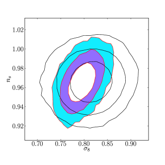
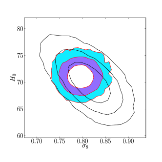
Figure 15: Contour plots of 2D probability distributions for fits using the WMAP7 data along with our new results for galaxy-galaxy lensing and galaxy clustering in SDSS, assuming flat $\Lambda$CDM. In all cases, we have marginalised over the nuisance parameters (bias and calibration) for our data, and over any cosmological parameters not shown on the plot. The black lines show $1$, $2$, and $3\sigma$ contours for WMAP7 alone. The contours shown in colour are WMAP7 and our data together. Top: $\sigma_{8}$ vs. $n_{s}$; bottom: $\sigma_{8}$ vs. $H_{0}$.

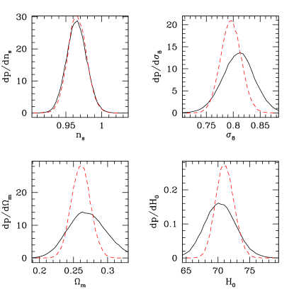
Figure 16: 1D probability distributions for fits using the WMAP7 data along with our new results for galaxy-galaxy lensing and galaxy clustering in SDSS, assuming flat $\Lambda$CDM as in Fig. 15. In all cases, we have marginalised over the nuisance parameters (bias and calibration) for our data, and over any cosmological parameters not shown on the plot. The solid black lines are for WMAP7 alone; red dashed lines are for WMAP7 and our data together.

Next, we allow the equation of state of dark energy ($w_{\mathrm{de}}$) to vary from a cosmological constant. Figs. 17 and 18 show 2D contours and 1D parameter distributions, respectively, and Table 4 gives best-fitting parameter constraints, again with WMAP7 alone (fit 8) and with our data included (fit 9). As in the $\Lambda$CDM case, our data do not provide significant additional constraining power on $n_{s}$, but it does improve the constraints on all the other parameters, most dramatically on $w_{\mathrm{de}}$ (because adding our data provides a constraint on the amplitude of matter fluctuations at times well after dark energy has become important).

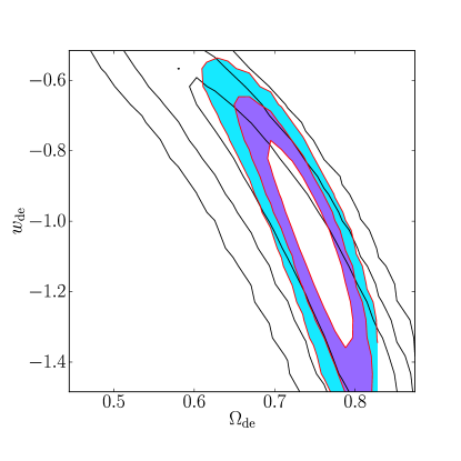
Figure 17: 2D contour plot for flat $w$CDM fits with the equation of state of dark energy allowed to vary from our fiducial value of $-1$ (but assumed to be constant in time). Line and contour styles are as in Fig. 15.

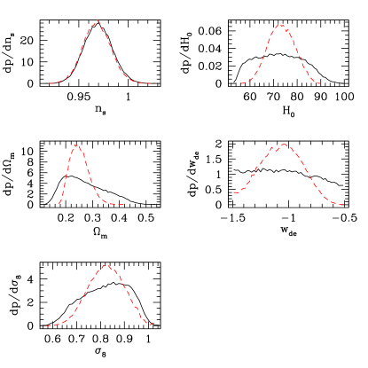
Figure 18: 1D probability distributions for flat $w$CDM fits with the equation of state of dark energy allowed to vary from our fiducial value of $-1$ (but assumed to be constant in time), as in Fig. 17. Line styles are as in Fig. 16.

Next, we relax the assumption of flatness (while still allowing the equation of state of dark energy to vary from a cosmological constant). Figs. 19 and 20 show 2D and 1D constraints, respectively, and Table 4 gives best-fitting parameter constraints, again with WMAP7 alone (fit 10) and with our data included (fit 11). We can see that with these relaxed assumptions about $w_{\mathrm{de}}$ and $\Omega_{k}$, the posterior probability distributions for $\Omega_{m}$, $H_{0}$, and $w_{\mathrm{de}}$ are very broad; our data play a crucial role in reducing the allowed region of parameter space for all parameters except $n_{s}$.

Finally, we revert to the assumption of flat $\Lambda$CDM, but we allow for the presence of massive neutrinos using the formalism in Sec. 2.3. Fig. 21 shows 1D posterior probability distributions and Table 4 gives best-fitting parameter constraints, again with WMAP7 alone (fit 12) and with our data included (fit 13). In addition to tightening constraints on $\sigma_{8}$, $\Omega_{m}$, and $H_{0}$ as before, our data help to rule out models with neutrino masses on the higher end of those allowed by WMAP7, such that the one-sided 95 per cent upper limit on neutrino mass goes down from 1.1 eV with WMAP7 alone to 0.56 eV with WMAP7 and our data. In general, the presence of massive neutrinos can significantly broaden the allowed parameter space for $\Omega_{m}$ and $H_{0}$ from CMB alone, and our data rule out some of the allowed high-$\Omega_{m}$ or low-$H_{0}$ values.

7.3 Comparison with previous work

The results of the previous section illustrate that our data provide cosmological parameter constraints that are consistent with and complementary to those from WMAP7. Here, we compare our constraints with those from other cosmological probes.

We do not compare our results against those from a pure clustering analysis of the shape and amplitude of the galaxy power spectrum, due to systematic uncertainties in treatments of non-linear galaxy bias, redshift-space distortions, and other issues. However, it is valuable to compare against measurements of baryonic acoustic oscillations (BAO), a measure of the expansion history of the universe rather than the growth of structure, since it is significantly less prone to such uncertainties. The most recent measurement of BAO in the SDSS DR7 (Mehta et al., 2012; Padmanabhan et al., 2012; Xu et al., 2012) represents the first use of the ‘reconstruction’ technique (Eisenstein et al., 2007) to reduce the effects of non-linear evolution of the density field in smoothing the BAO peak. Mehta et al. (2012) demonstrates that when combining the BAO peak position with CMB data, they find $\Omega_{m}=0.280\pm 0.014$ (in the context of flat $\Lambda$CDM). This result is fully consistent with our data when fitting for $\sigma_{8}$ and $\Omega_{m}$, which yielded $\Omega_{m}=0.257^{+0.038}_{-0.034}$ (Sec. 7.1). This consistency is non-trivial, given that the BAO results use an identical sample to make a fully geometric constraint on cosmology, whereas we measure the amplitude of clustering well below the BAO peak.

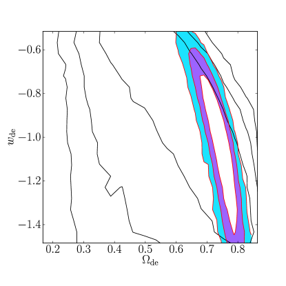
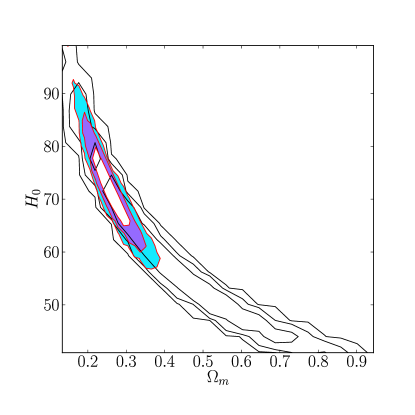
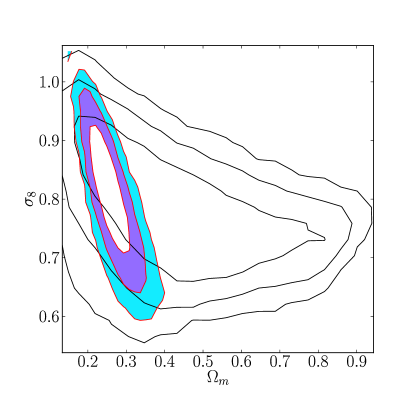
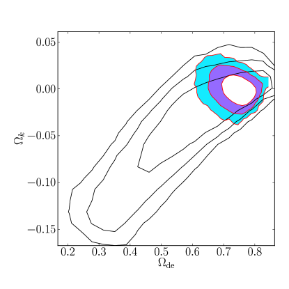
Figure 19: 2D contour plot for $w$CDM fits without the assumption of flatness. Line and contour styles are as in Fig. 15.

We can also compare against the BAO results from the Baryon Oscillation Spectroscopic Survey (BOSS) presented in Anderson et al. (2012). Assuming flat $\Lambda$CDM, when using WMAP7 and the BAO results for two galaxy samples, they find $\Omega_{m}=0.293\pm 0.012$ and $H_{0}=68.8\pm 1.0$ km s^-1 Mpc^-1. We compare this with our fit 7 (combining our data with WMAP7), which gave $\Omega_{m}=0.261\pm 0.014$ and $H_{0}=71.1\pm 1.5$ km s^-1. A naive comparison of the results – neglecting the fact that both measurements include WMAP7 – suggests a $1.7\sigma$ and $1.3\sigma$ discepancy for $\Omega_{m}$ and $H_{0}$, respectively. While these are not very significant, the tension is in fact worse since a significant part of the constraining power comes from the CMB data, which is the same for both measurements. We defer exploration of this possible tension between the BAO and our lensing constraints to future work; however, we note that fit 13 suggests that including the effects of massive neutrinos would help to reduce this tension.

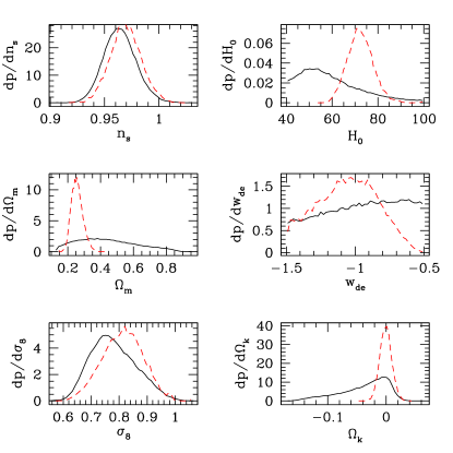
Figure 20: 1D probability distributions for $w$CDM fits without the assumption of flatness, as in Fig. 19. Line styles are as in Fig. 16.

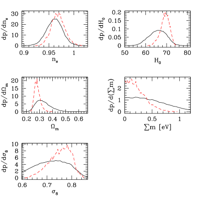
Figure 21: 1D probability distributions for flat $\Lambda$CDM fits with massive neutrinos. Line styles are as in Fig. 16.

We also compare our results against those from other lensing analyses, particularly cosmic shear. First, we compare against those from the COSMOS survey, including the original analysis from Massey et al. (2007) and a re-analysis in Schrabback et al. (2010). The results from Massey et al. (2007) used a 3D analysis to infer $\sigma_{8}(\Omega_{m}/0.3)^{0.44}=0.866^{+0.085}_{-0.068}$ (68 per cent CL, stat. $+$ sys.). We can compare this result against our result when fitting for $\sigma_{8}$ and $\Omega_{m}$, $\sigma_{8}(\Omega_{m}/0.25)^{0.57}=0.80\pm 0.05$ marginalised over nuisance parameters. The COSMOS results are $\sim 1.6\sigma$ above ours, giving a higher amplitude of clustering. The 3D COSMOS lensing analysis in Schrabback et al. (2010) gives, for flat $\Lambda$CDM, a value $\sigma_{8}(\Omega_{m}/0.3)^{0.51}=0.75\pm 0.08$, consistent with our results at the $\sim 0.2\sigma$ level. Part of the reason for the lower quoted clustering amplitude in Schrabback et al. (2010) is a different treatment of the non-linear power spectrum (more consistent with ours): if they use the same treatment as Massey et al. (2007), they find $0.79\pm 0.09$, higher by 5 per cent. Other differences in clustering amplitude between the two COSMOS results could come from the different treatment of PSF estimation, charge-transfer inefficiency, the availability of more photometric data to improve the photometric redshifts, or differences in analysis methods (scales used and so on). In short, the COSMOS lensing results are consistent with ours, with the exact comparison depending on the method of analysis and the treatment of systematic errors.

We can also compare against cosmic shear results from stripe 82 of the SDSS itself. There are two such results that use largely independent analysis methods on the same data, by Huff et al. (2011) and Lin et al. (2012). The work in Huff et al. (2011) used the same PSF correction technique as we have used, and also the same simulation method relying on space-based training data (Mandelbaum et al., 2012) to calibrate the shape measurements, so its systematic errors may not be fully independent from ours. However, given that the area of stripe 82 is $\sim 3$ per cent of the area used here, we can consider those results to be statistically independent of ours. With fixed $\Omega_{m}$ close to our value, Huff et al. (2011) find a relatively low amplitude of matter fluctuations, $\sigma_{8}=0.636^{+0.109}_{-0.154}$, which can be compared with our $0.80\pm 0.05$. Assuming completely independent errors, this represents a $1.4\sigma$ discrepancy, which is not statistically significant mainly due to the small size of stripe 82 and the limited source number density due to the SDSS seeing. Comparing with Lin et al. (2012), they find for flat $\Lambda$CDM that $\sigma_{8}\Omega_{m}^{0.7}=0.252^{+0.032}_{-0.052}$. For our value of $\Omega_{m}=0.25$, that constraint becomes $\sigma_{8}=0.665^{+0.084}_{-0.137}$, quite similar to that from Huff et al. (2011). In both cases we therefore see a slight tension with our results, but only at the $\sim 1.4\sigma$ level.

We also compare against the most recent cosmic shear results from the Canada-France-Hawaii Telescope Legacy Survey (CFHTLS), presented in Heymans et al. (2013). The sample in this analysis covers 154 deg² and has a median redshift of $z_{\rm med}=0.70$. After computing tomographic cosmic shear signals and marginalizing over a model for intrinsic alignments, they find a best-constrained parameter combination of $\sigma_{8}(\Omega_{m}/0.27)^{0.46\pm 0.02}=0.774^{+0.032}_{-0.041}$ before combining with any external datasets. This result is completely consistent with our findings of $\sigma_{8}(\Omega_{m}/0.25)^{0.57}=0.80\pm 0.05$.

Finally, we compare our results with those from analyses that used small-scale lensing and clustering measurements, despite our caveats from Sec. 2. First, Cacciato et al. (2012a) carried out a joint lensing and clustering analysis of SDSS ‘Main’ sample galaxies to constrain cosmology. They employed the alternate approach, discussed briefly in Sec. 2, of using the measurements to small scales, which requires use of an HOD model for how galaxies populate dark matter halos in order to interpret the measurements. Despite use of SDSS data, that measurement is somewhat independent of this one because it (a) uses a subset of the area and (b) employs smaller scales than this one. Their results for the flat $\Lambda$CDM model with WMAP7 priors on $n_{s}$, $h$, and $\Omega_{b}$ are consistent with ours, $\Omega_{m}=0.278^{+0.023}_{-0.026}$ and $\sigma_{8}=0.763^{+0.064}_{-0.049}$ (95 per cent CL). Second, we compare with the results from Tinker et al. (2012), who used the mass-to-number ratio for galaxy clusters combined with the mass versus richness calibration based on weak lensing, and the galaxy clustering (using an HOD). These measurements should be somewhat but not highly correlated with ours, because of the different range of scales used. For their combination of observables and modeling method, they find $\sigma_{8}\Omega_{m}^{0.5}=0.465\pm 0.026$, or $\sigma_{8}(\Omega_{m}/0.25)^{0.5}=0.93\pm 0.05$ ($1\sigma$). Compared with our result of $\sigma_{8}(\Omega_{m}/0.25)^{0.57}=0.80\pm 0.05$, there is clearly some tension, since the discrepancy is $2.5\sigma$ assuming independent errors, and in fact there should be some correlation between the results. Understanding the exact source of this tension is beyond the scope of this work, but likely it lies in the different assumptions behind the methods. We also note that when combining with CMB data, they find $\Omega_{m}=0.290\pm 0.016$ and $\sigma_{8}=0.826\pm 0.020$, which should be compared with our flat $\Lambda$CDM results of $\Omega_{m}=0.270^{+0.030}_{-0.027}$ and $\sigma_{8}=0.810\pm 0.029$. Here, the tension is less evident, presumably because of the combination with identical CMB data.

8 Discussion

We have used updated measurements of galaxy-galaxy weak lensing and galaxy clustering for several samples of spectroscopic galaxies in the SDSS DR7 to place competitive constraints on the amplitude of matter fluctuations and, by combining with WMAP7 data, the growth of structure with time. The novelty in comparison with previous lensing cosmology constraints is that we have used galaxy-galaxy lensing (a cross-correlation of lens galaxy positions and the background shear field) rather than cosmic shear (the auto-correlation of the shear field). From a statistical perspective, the former is more detectable in low-redshift surveys such as SDSS; however, even at higher redshift, the galaxy-galaxy lensing typically has a lower systematic error budget, because the use of cross-correlations allows us to more easily remove several systematic errors (intrinsic alignments, additive shear systematics) that plague cosmic shear. To avoid contamination from the smallest scales, where there are uncertainties in the galaxy-mass cross-correlation due to the way that galaxies populate halos, we have used the annular differential surface density (ADSD) statistic $\Upsilon$, which strictly removes contributions below some scale $R_{0}$ (chosen based on comparison with simulations to be $4$$h^{-1}\mathrm{Mpc}$ for the clustering analysis, and $2$$h^{-1}\mathrm{Mpc}$ for the lensing analysis). We apply this approach to three different non-overlapping samples extracted from SDSS DR7: an intermediate redshift ($0.16<z<0.36$) LRG sample, high redshift ($0.36<z<0.47$) LRG sample, and a low redshift sample ($z<0.155$) with a fainter absolute magnitude limit and no colour selection. We have opted to model the signals using the non-linear matter power spectrum along with a perturbation theory-based model for the non-linear galaxy bias, containing parameters over which we marginalise. We see clear evidence for a scale-dependent bias in our LRG sample with large-scale bias around $2$, while there is no evidence for the scale-dependent bias for the lower luminosity sample with large-scale bias around $1.25$. This trend is consistent with theoretical expectations based on simulations and analytic predictions (Baldauf et al., 2012).

Using our data and fixing all cosmological parameters except for $\sigma_{8}$ and $\Omega_{m}$, we find $\sigma_{8}(\Omega_{m}/0.25)^{0.57}=0.80\pm 0.05$ ($1\sigma$, stat. $+$ sys.) after marginalising over the galaxy bias parameters and a nuisance parameter for the lensing calibration. This result is highly consistent with that from the WMAP7 CMB analysis, and with many other cosmological measurements as discussed in Sec. 7.3. The 6 per cent errorbar, including both statistical and systematic contributions, indicates that the SDSS is a quite powerful survey for weak lensing cosmology at low redshift (in the context of other extant lensing datasets). Moreover, given its low effective redshift of $\sim 0.27$, we imagine future benefits from the combination with other lensing measurements that typically have higher effective redshifts.

When we include WMAP7 data in the analysis, we find that for flat $\Lambda$CDM, we are able to provide significant additional constraining power on $\sigma_{8}$, $\Omega_{m}$, and $H_{0}$ due to orthogonal degeneracy directions, effectively halving the allowed region in parameter space; we do not provide significant additional constraining power on $n_{s}$. When we allow the equation of state of dark energy $w_{\mathrm{de}}$ to vary from $-1$ (while still assuming it is constant in time), when we further allow the possibility of curvature, or when we include massive neutrinos in the context of flat $\Lambda$CDM, we likewise find that our low-redshift constraint on the amplitude of matter fluctuations is crucial for reducing major parameter degeneracies. It will be interesting to combine these results with a low-redshift constraint on the expansion history of the universe, such as from BAO; we defer this exercise to future work, but note that Section 7.3 suggests that inclusion of massive neutrinos may be necessary to reduce some tension between constraints on $\Omega_{m}$ and $H_{0}$ from the two probes.

We emphasise that these results represent an entirely new opportunity for the field of lensing to constrain cosmological parameters in a way that is largely independent of the details of how galaxies populate dark matter halos, but also less sensitive than cosmic shear to several important observational and astrophysical systematic errors. Among these are all additive contributions such as telescope or atmosphere effects that induce shear-shear correlations but not shear-galaxy correlations. Intrinsic alignments also do not contribute to shear-galaxy correlations as long as the redshift separation between lenses and sources, using photometric redshift information, is effective. In contrast, the dominant intrinsic alignment contribution to shear-shear correlations, induced by correlations between sheared galaxies in the background and intrinsically-aligned galaxies in the foreground, cannot be eliminated simply by using photometric redshift information (Hirata & Seljak, 2004).

In addition to the intrinsic value of these cosmological constraints in and of themselves, this work is a proof of concept for this analysis technique for the next generation of large, wide-field surveys that will carry out lensing measurements, such as Hyper Suprime-Cam (HSC, Miyazaki et al. 2006), Dark Energy Survey (DES, The Dark Energy Survey Collaboration 2005), the KIlo-Degree Survey (KIDS), the Panoramic Survey Telescope and Rapid Response System (Pan-STARRS, Kaiser et al. 2010); and even more ambitious programmes such as the Large Synoptic Survey Telescope (LSST, LSST Science Collaborations et al. 2009), Euclid, and the Wide-Field Infrared Survey Telescope (WFIRST). The ability to make cosmological measurements with galaxy-galaxy lensing rather than cosmic shear is particularly important for making use of early data from upcoming surveys, when additive shear systematics will be less well-understood. We expect that this approach will yield results that are competitive and complementary to shear-shear analysis for these future surveys as well.

The data used for the cosmological parameter constraints, and the MCMC chains, can be downloaded directly from the first author’s website.

Appendix A Calibration of the method

As a basic test, we use the data from the simulated LRG sample (Sec. 2.1) and check whether we can accurately recover the input cosmology using the analysis framework from Sec. 2.3. Such tests with various $R_{0}$ will allow us to determine the safest choice of $R_{0}$ to minimise systematic error without excessively increasing the statistical errors.

For this test, we fixed all cosmological parameters besides $\sigma_{8}$, and varied $R_{0}$, making sure that we can recover the true $\sigma_{8}=0.8$ for the simulations. While doing this test, we allowed the lensing calibration and the bias parameters to be free parameters. Given that moving $R_{0}$ above 2$h^{-1}\mathrm{Mpc}$ for the galaxy-galaxy lensing severely impacts the $S/N$, we consider only this value of $R_{0}$ for the lensing, but vary $R_{0}$ for the clustering from 2 to 6$h^{-1}\mathrm{Mpc}$, in steps of 2$h^{-1}\mathrm{Mpc}$. This procedure is also theoretically motivated since, as pointed out in Sec. 2.4, the clustering signal should be more strongly sensitive than the g-g lensing signal to the details of how galaxies occupy dark matter halos on these scales. Shape noise was not added to the simulated LRG data, and the simulation volume is 40 times larger than the cosmological volume covered by the real data. Thus, the cosmic variance is substantially smaller than that in the real data, and in any case, our dominant source of noise (shape noise) is not present. Because of this, we can trust the simulations to reveal low-level biases due to our fitting procedure, at the level of $\sim 0.2\sigma$ (where $\sigma$ is the statistical uncertainty in the cosmological parameters in the fits to real data). For $R_{0,\mathrm{g}\mathrm{g}}=2,4,6$$h^{-1}\mathrm{Mpc}$, the best-fitting $\sigma_{8}=0.763,0.795,0.792$ (these are the global best-fit values, not marginalised over nuisance parameters). The first value, for $R_{0,\mathrm{g}\mathrm{g}}=2$$h^{-1}\mathrm{Mpc}$, indicates a statistically-significant bias in $\sigma_{8}$. However, the results for larger $R_{0}$ are consistent with no bias, so we adopt $R_{0}=2$$h^{-1}\mathrm{Mpc}$ and $4$$h^{-1}\mathrm{Mpc}$ for the g-g lensing and galaxy clustering, respectively. The fact that the most likely point agrees with the theory means that there is no inherent bias in the theory predictions with respect to our simulations.

We can also check the effect of priors and marginalisation over lensing calibration bias and galaxy bias parameters. After marginalisation over the galaxy bias parameters and the lensing calibration, the median of the likelihood is $0.78$, which differs from the input value and the global best-fitting value of 0.8. Since our best fit model (maximum likelihood) is at the position of the input model, the discrepancy between the median and the input value must be due to the effect of the priors and the marginalisation process. The median is the standard value quoted in the Markov Chain Monte Carlo (MCMC) analyses, since it can be robustly estimated. It is also invariant under a monotonic transformation of the variable, i.e. the median of $\sigma_{8}$ is the same as the median of $\sigma_{8}^{2}$ assuming the same prior, which is believed to be useful since there is no good reason a priori to use the linear fluctuation amplitude $\sigma_{8}$ as opposed to the correlation function amplitude $\sigma_{8}^{2}$. However, this does not mean that the median is invariant under the change of the prior, i.e. if we start with a uniform prior on $\sigma_{8}$ we obtain a different median than if we use a uniform prior on $\sigma_{8}^{2}$. The only number that is prior-independent is the maximum likelihood value, which is unstable in multi-dimensional MCMC analyses, since the likelihood surface is shallow and MCMC has difficulties finding the absolute maximum with a finite number of steps. It is nevertheless convenient that the main reported number agrees with the input value in simulations. Since a prior that is uniform in $\sigma_{8}$ does not result in this property, and since there is nothing especially natural about that choice of the prior, we will empirically choose a prior such that the median $\sigma_{8}$ agrees with the input value in simulations, and then report the median determined in a similar way in the data. If we apply a flat prior on $\sigma_{8}^{5}$, the median increases to $\sigma_{8}=0.80$, and since this agrees with the input value we adopt this prior for the rest of the paper. Note that as we add more data, such as additional SDSS datasets (we use three samples, not just LRGs as in the tests in this section) and WMAP, the effect of the prior is diminished and we converge on the true value. This is the reason to apply a prior, rather than a correction factor such as $0.80/0.78$, which would have an excessive impact in the case where we add more data.

The plots of simulated $\Upsilon$ are shown in Fig. 2, and we see that the simulated data and the best model agree reasonably well both for galaxy-galaxy lensing and galaxy clustering, with $b_{2}=0.25$ as the best fit value.

We also note that in the real data, when carrying out the fitting procedure, we see a qualitatively similar trend in $\sigma_{8}(R_{0,\mathrm{g}\mathrm{g}})$ increasing with $R_{0}$, however the change in $\sigma_{8}$ is larger in amplitude (but consistent with that given here within the errors). As a final sanity check of our procedure above, we carry out the analysis using another HOD sample, constructed from simulations with $\sigma_{8}=0.90$ and selected to mimic a higher-luminosity and higher-mass sample. For this HOD sample, with our adopted values of $R_{0}$ for g-g lensing and galaxy clustering and our prior on $\sigma_{8}$, we find best-fitting and median $\sigma_{8}=0.90$ and $0.92$. The former number is completely consistent with the input cosmological model, reassuring us that our choice of $R_{0}$ is robust to significant changes in the galaxy mass and input cosmology. The latter number suggests that for large values of $\sigma_{8}$, the adopted prior will cause a bias that is $\sim 40$ per cent of our statistical errors. However, we see no evidence for such a high $\sigma_{8}$, and so this worst-case scenario is not an issue in practise.

Appendix B Weak lensing systematics tests

In this Appendix, we present several tests of systematic error in the lensing signals, focusing exclusively on those tests that were not done for the same shape catalogue by R12.

B.1 Calculation of $\Upsilon_{\mathrm{g}\mathrm{m}}$

Since we use $\Upsilon_{\mathrm{g}\mathrm{m}}$ for cosmological parameter constraints, and it is a derived quantity that relies on determination of $\Delta\Sigma(R_{0})$, here we present tests illustrating the accuracy of that determination.

As stated in Sec. 4.1, we determine $\Delta\Sigma(R_{0})$ using power-law fits over a range of scales on which $\Delta\Sigma$ appears consistent with a power-law, including $R_{0}$ itself to avoid extrapolation. In Fig. 22, we show (for all three samples) the observed $\Delta\Sigma(R)$ divided by the best-fit power-law for the chosen range of scales which are indicated by vertical lines. This power-law is determined from a fit to the jackknife mean $\Delta\Sigma$, weighted by the inverse variance (assumed to be diagonal, which is appropriate for these scales). Ideally, this ratio of observed signal to power-law would be consistent with one for all scales between the vertical lines. In addition, we show the jackknife mean value of $\Delta\Sigma(R_{0})$ and its jackknife errorbar, again with respect to the best-fit power-law for the chosen range of scales and therefore with an ideal value of $1$. It is clear that the power-law approximation is valid on the range of scales used, but the observed signal deviates from it strongly outside of that range. This power-law fit is used only for empirical determination of $\Delta\Sigma(R_{0})$, not for any other purpose.

The best-fit power-laws and ranges of scales used are defined as $\Delta\Sigma=\Delta\Sigma_{0}(R/R_{0})^{\alpha}$ for $R_{\mathrm{pow,min}}<R<R_{\mathrm{pow,max}}$, where $\Delta\Sigma_{0}$ is in units of $hM_{\odot}/\mathrm{pc}^{2}$. Given this definition, the power-laws that went into Fig. 22 are described in Table 5.

Sample	$R_{\mathrm{pow,min}}$	$R_{\mathrm{pow,max}}$	$\Delta\Sigma_{0}$	$\alpha$
	$[$$h^{-1}\mathrm{Mpc}$$]$	$[$$h^{-1}\mathrm{Mpc}$$]$	$[hM_{\odot}/\mathrm{pc}^{2}]$
Main-L5	0.2	7.0	$2.49$	$-0.97$
LRG	0.5	8.5	$5.81$	$-1.22$
LRG-highz	0.2	8.5	$5.41$	$-1.08$

Table 5: Best-fitting power-law functions (as defined in Sec. B.1) to $\Delta\Sigma(R)$ for a limited range of scales, used to estimate $\Delta\Sigma(R_{0})$ and therefore $\Upsilon_{\mathrm{g}\mathrm{m}}$.

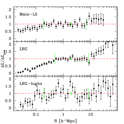
Figure 22: Lensing signals for the three samples (as labelled on the plot) divided by the best-fit power-law using the range of scales indicated by vertical solid lines. The horizontal dashed line shows the ideal value $\Delta\Sigma/\Delta\Sigma_{\mathrm{pow}}=1$. Also, a single point shown as an $\times$ with its own errorbar at $R_{0}=2$$h^{-1}\mathrm{Mpc}$ shows the jackknife mean value that was used for $\Delta\Sigma(R_{0})$, and its jackknife error.

B.2 Correction for physically associated sources

The boost factors (Eq. 33) that implicitly went into those signals are shown in Fig. 23. As shown, the correction is very small ($\sim$ per cent level) on the scales used for this measurement, $\gtrsim 2h^{-1}$Mpc. The size of the errorbars indicates that there are $\sim 1$ per cent-level density fluctuations in the real catalogue on large scales, perhaps due to dependence of the lens number density on systematics that are not properly reproduced in the random catalogues. This does not bias the lensing signal, it simply acts as a minor contribution to the statistical error budget, subdominant to shape noise.

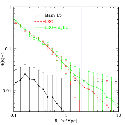
Figure 23: Boost factors $B(R)-1$ as a function of separation for the three samples used in this analysis, as labeled on the plot. The vertical solid line at $R=2h^{-1}$Mpc indicates the physical scales used for the cosmological constraints in this paper.

B.3 Intrinsic alignments

We must consider the contribution of intrinsic alignments to our measurement. In principle, they should only contribute if photo-$z$ errors scatter galaxies that are actually physically-associated with our lenses into the source sample, and if those physically-associated galaxies have a tendency to align radially or tangentially with respect to our lenses. In principle, we expect a radial alignment for elliptical galaxies, which should follow the linear alignment model to some extent (Hirata & Seljak, 2004); this alignment has been observed (e.g., Hirata et al., 2007) but primarily for bright red galaxies, rather than the faint ones that we use as sources in our lensing analysis. Disk galaxies are expected to align in a way that relates their disk angular momentum to the dark matter halo angular momentum, which leads to essentially no net radial or tangential alignment with respect to lens galaxies (Hirata & Seljak, 2004).

Thus, our approach here is to assume that blue sources, which contribute $\sim 70$ per cent of the weight to the lensing measurement, contribute zero intrinsic alignment, and red sources contribute some amount that we must empirically constrain. A method for carrying out this empirical constraint is presented in Blazek et al. (2012); it relies on calculating shears of sources selected in different photo-$z$ bins with respect to the lenses. That work shows that using this method, we can constrain intrinsic alignment contamination of the galaxy-galaxy lensing signal at 10$h^{-1}\mathrm{Mpc}$ (the scale which roughly dominates our lensing constraints) to $<2$ per cent, for our LRG lens sample (which has the lowest statistical error and therefore is the most demanding in terms of systematics). Assuming that $\sim 30$ per cent of the source sample has at most a 2 per cent intrinsic alignment contamination, this translates to $<0.6$ per cent intrinsic alignment contamination of our lensing signals. This is far subdominant to our other assumed systematic errors (e.g., 4-5 per cent for lensing calibration), so we assume it is negligible for the purpose of these cosmological constraints.

B.4 Ratio test

As described in Sec. 4.2.1, we apply a number of corrections for known sources of calibration bias such as photo-$z$ error. To support the claim that we understand these effects well, we carry out ratio tests of the signals computed using the same lens sample and different source samples. After correcting for known calibration biases that are different for each sample, these ratios should simply be consistent with one within the errors (which are typically $\pm 0.06$).

There are several ratio tests that we can carry out, each of which is sensitive to our understanding of several effects. For example, when dividing the sample into red and blue galaxies, we are most sensitive to differences in photo-$z$ errors and to differences in the intrinsic ellipticity distribution of the red and blue galaxy populations. When dividing into faint versus bright galaxies, we are most sensitive to noise rectification bias and photo-$z$ errors in the former. When dividing into well- vs. poorly-resolved galaxies, we are most sensitive to selection biases that couple the shear to the apparent size. When dividing into all sources vs. only those with $z_{\mathrm{phot}}>0.45$, we are most sensitive to photo-$z$ errors in the former (the photo-$z$ errors in the latter are less important because of the larger redshift separation between lenses and sources). Therefore, an ability to achieve a ratio of one in each of these four cases would suggest that we understand the different systematic errors that are affecting the lensing signals in each case well enough to constrain cosmology at the $\sim 5$ per cent level.

Our findings, using the LRG lens sample, is that in three cases the ratio is within $1\sigma$ of one. In the final case, the split into red versus blue sources, the ratio is $0.92\pm 0.06$; thus the discrepancy is only a little more than $1\sigma$, and since we expect such a case to turn up after doing several ratio tests, we conclude that the ratio tests do not indicate any major misunderstanding of the predominant systematic errors affecting the lensing calibration.

B.5 Large-scale systematic shear

In this section, we present tests of the large-scale shear systematics. As noted in Mandelbaum et al. (2005), the presence of a coherent PSF ellipticity along the scan direction in the SDSS data can result in a non-zero tangential shear on large scales, where lens-source pairs may be lost due to survey edge effects. There, we corrected for this effect by subtracting off the g-g lensing signal around random points, but also noted that if the systematic shear correlates in some way with the lens number density, this correction may not be sufficient. Thus, we must test the accuracy of this procedure when using large-scale lensing signals to constrain cosmology.

In Fig. 24, we show the g-g lensing signal around random points for our three lens samples. As shown, it becomes significantly inconsistent with zero for scales above $10$, $20$, and $15h^{-1}$Mpc for Main-L5, LRG, and high-$z$ LRG, respectively. The reason for the different scales is that it is a systematic associated with an angular scale, which becomes different physical scales when we convert angular separation $\theta$ to $R$ at the different typical lens redshifts. However, its magnitude also depends on the apparent magnitude and resolution factors of sources used, as we have confirmed explicitly by dividing our source sample by source properties. These two effects go in competing directions, driving the typical scale of the systematic error to increasing $R$ as $z$ increases, then at a certain point above $z\sim 0.3$, the typical scale starts to decrease again. For reference, this figure also shows the observed signal around real lenses in the same form ($R\Delta\Sigma$), to show at which point the systematic correction is comparable in size. Generally, on the maximum scale used for science, the systematic correction ranges from $1/3$ to $1/2$ of the real signal, and is $1$–$2$ times larger than the statistical error.

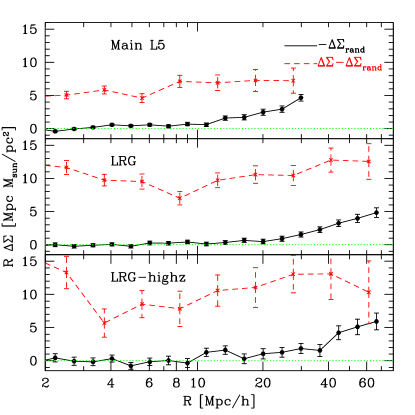
Figure 24: The black points and lines show $-R\Delta\Sigma_{\mathrm{rand}}$, a measure of systematic shear in the source catalogue. Each panel is a different sample (Main L5, LRG, LRG-highz from top to bottom). For reference, the actual signal that we use for science is also shown as the red dashed lines.

Given the significance of this systematics signal on the largest scales used for our measurements, we must assess whether the assumptions behind the correction for it are correct (c.f. Sec. 4.2). In order to do so, we rely on the following facts: First, if there is some coherent systematic shear, then depending on the survey geometry, it can also show up as a signal in the other shear component $\gamma_{\times}$ on large scales. Second, there is no gravitational lensing signal in that shear component. Thus, we measure $\Delta\Sigma_{\times}$ around real lenses and $\Delta\Sigma_{\times,\mathrm{rand}}$ around random points, and check to see whether they are consistent. An inconsistency would call into question the validity of this correction using random points.

As shown in Fig. 25 for one of the lens samples, we find that there is a significant signal in the $\times$ shear component on the same scales as for the $+$ component, and $\Delta\Sigma_{\times,\mathrm{rand}}\approx 1.25\Delta\Sigma_{\times}$ (actually it is $\sim 1.2\Delta\Sigma_{\times}$ on this Figure; $1.25$ is the result if we average over all the lens samples to reduce the noise). Taken at face value, this suggests that the systematic shear correlates with some factor that determines the effective lens number density, and that correlation is not properly taken into account by our procedure for producing random catalogues. This finding is also consistent with the results in Sec. B.2. There is likely a simple physical explanation for this issue related to the data processing; for example, very slight correlations of lens selection probability with the PSF FWHM, extinction, or sky level should also correlate with fluctuations in the systematic shear in the sources.

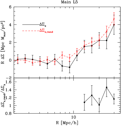
Figure 25: Top: The black solid and red dashed lines show $R\Delta\Sigma_{\times}$ and $R\Delta\Sigma_{\times,\mathrm{rand}}$, respectively, for the Main L5 sample. Bottom: For the scales that have a significant systematic shear signal, we show the ratio $\Delta\Sigma_{\times,\mathrm{rand}}/\Delta\Sigma_{\times}$.

We consider the implications for the LRG sample, as an example. That sample has $\Delta\Sigma\sim 0.30\pm 0.03$ and $\Delta\Sigma_{\mathrm{rand}}\sim-0.10$ at 50$h^{-1}\mathrm{Mpc}$. If we assume that $\Delta\Sigma_{\mathrm{rand}}$ is overestimating the true systematic shear by a factor of 1.25, then that means we should have been subtracting $-0.08$, not $-0.10$, from the original signal to get our final $\Delta\Sigma$. Thus, our original $\Delta\Sigma$ should have been $0.28\pm 0.03$, a shift of $(2/3)\sigma$. The size of this correction compared to the statistical error suggests that we should impose the correction by simply dividing $\Delta\Sigma_{\mathrm{rand}}$ by 1.25 before subtracting it to get our estimate of the lensing signal. Indeed, we applied corrections in this way to all signals used for science and shown in all plots in this paper.

As an additional test, we computed the signal while excluding all LRGs within $60$$h^{-1}\mathrm{Mpc}$ of a survey edge. The resulting systematic shear signal was consistent with zero, and the value of $\Delta\Sigma$ was unchanged on average on small scales, and decreased at the expected level on the largest scales. However, we merely present this test to validate our correction scheme; we do not use the signal with survey edges removed for science, because the statistical errors on a few $h^{-1}\mathrm{Mpc}$ scales increase significantly (20 per cent).

Finally, we note that a non-negligible fraction of this systematic shear signal ($\sim 30$–$40$ per cent) is due to an error in the SDSS PSF model identified in R12, which resulted in all PSF models in the $r$ band in one of the camera columns having some spurious ellipticity. The remainder is due to the inadequacy of the adopted PSF correction method at removing the PSF ellipticity from the galaxy shapes.

Appendix C Galaxy clustering systematics tests

C.1 Calculation of $\Upsilon_{\mathrm{g}\mathrm{g}}$

Since we use $\Upsilon_{\mathrm{g}\mathrm{g}}$ for our cosmological parameter constraints, and it is a derived quantity that relies on determination of $w_{\mathrm{g}\mathrm{g}}(R_{0})$, here we present tests illustrating the accuracy of that determination.

As for the lensing signal $\Delta\Sigma$, we determine $w_{\mathrm{g}\mathrm{g}}(R_{0})$ using power-law fits over a range of scales including $R_{0}$ on which $w_{\mathrm{g}\mathrm{g}}$ appears consistent with a power-law. In Fig. 26, we show (for all three samples) the observed $w_{\mathrm{g}\mathrm{g}}(R)$ divided by the best-fit power-law for the chosen range of scales which are indicated by vertical lines. This power-law is determined from a fit to the jackknife mean $w_{\mathrm{g}\mathrm{g}}$, weighted by the inverse variance (assumed to be diagonal on these scales). Ideally, this ratio of observed signal to best-fit power law would be consistent with one between the vertical lines. It is clear that the power-law approximation is valid on the range of scales used, but the observed signal deviates from it strongly outside of that range, which is what we expect for $\Lambda$CDM and typical models of scale-dependent bias.

The best-fit power-laws and ranges of scales used are defined as $w_{\mathrm{g}\mathrm{g}}=w_{0}(R/R_{0})^{\beta}$ for $R_{\mathrm{pow,min}}<R<R_{\mathrm{pow,max}}$, where $w_{0}$ is in units of $h^{-1}\mathrm{Mpc}$. Given this definition, the power-laws that went into Fig. 26 are given in Table 6.

Sample	$R_{\mathrm{pow,min}}$	$R_{\mathrm{pow,max}}$	$w_{0}$	$\beta$
	$[$$h^{-1}\mathrm{Mpc}$$]$	$[$$h^{-1}\mathrm{Mpc}$$]$	$[$$h^{-1}\mathrm{Mpc}$$]$
Main-L5	2.0	8.0	$35.4$	$-0.71$
LRG	1.0	9.0	$75.7$	$-0.83$
LRG-highz	1.0	4.0	$88.0$	$-0.64$

Table 6: Best-fitting power-law functions (as defined in Sec. C.1) to $w_{\mathrm{g}\mathrm{g}}(R)$ for a limited range of scales, used to estimate $w_{\mathrm{g}\mathrm{g}}(R_{0})$ and therefore $\Upsilon_{\mathrm{g}\mathrm{g}}$.

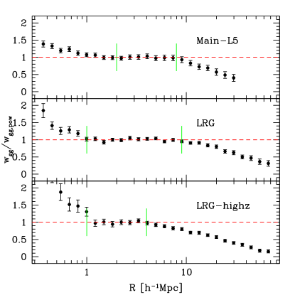
Figure 26: Clustering signals for the three samples (as labelled on the plot) divided by the best-fit power-law using the range of scales indicated by vertical solid lines. The horizontal dashed line shows the ideal value $w_{\mathrm{g}\mathrm{g}}/w_{\mathrm{gg,pow}}=1$.

References

- Abazajian et al. (2009) Abazajian K. et al., 2009, ApJS, 182, 543
- Aihara et al. (2011) Aihara H. et al., 2011, ApJS, 193, 29
- Albrecht et al. (2006) Albrecht A. et al., 2006, preprint (astro-ph/0609591)
- Anderson et al. (2012) Anderson L. et al., 2012, MNRAS, 427, 3435
- Bacon et al. (2000) Bacon D. J., Refregier A. R., Ellis R. S., 2000, MNRAS, 318, 625
- Baldauf et al. (2010) Baldauf T., Smith R. E., Seljak U., Mandelbaum R., 2010, Phys. Rev. D, 81, 063531
- Baldauf et al. (2012) Baldauf T., Seljak U., Desjacques V., McDonald P., 2012, Phys. Rev. D, 86, 083540
- Bartelmann & Schneider (2001) Bartelmann M., Schneider P., 2001, Phys. Rep., 340, 291
- Bernardeau et al. (2002) Bernardeau F., Colombi S., Gaztanaga E., Scoccimarro R., 2002, Phys. Rep., 367, 1
- Bernstein & Jarvis (2002) Bernstein G. M., Jarvis M., 2002, AJ, 123, 583
- Bird et al. (2012) Bird S., Viel M., Haehnelt M. G., 2012, MNRAS, 420, 2551
- Blanton et al. (2001) Blanton M. R. et al., 2001, AJ, 121, 2358
- Blanton & Roweis (2007) Blanton M. R., Roweis S., 2007, AJ, 133, 734
- Blanton et al. (2005) Blanton M. R. et al., 2005, AJ, 129, 2562
- Blazek et al. (2012) Blazek J., Mandelbaum R., Seljak U., Nakajima R., 2012, JCAP, 5, 41
- Bridle et al. (2010) Bridle S. et al., 2010, MNRAS, 405, 2044
- Cacciato et al. (2009) Cacciato M., van den Bosch F. C., More S., Li R., Mo H. J., Yang X., 2009, MNRAS, 394, 929
- Cacciato et al. (2012a) Cacciato M., van den Bosch F. C., More S., Mo H., Yang X., 2012a, preprint (arXiv:1207.0503)
- Cacciato et al. (2012b) Cacciato M., Lahav O., van den Bosch F. C., Hoekstra H., Dekel A., 2012b, MNRAS, 426, 566
- Chan et al. (2012) Chan K. C., Scoccimarro R., Sheth R. K., 2012, Phys. Rev. D, 85, 083509
- Cole et al. (2005) Cole S. et al., 2005, MNRAS, 362, 505
- Davis et al. (1985) Davis M., Efstathiou G., Frenk C. S., White S. D. M., 1985, ApJ, 292, 371
- Dekel & Lahav (1999) Dekel A., Lahav O., 1999, ApJ, 520, 24
- Eisenstein et al. (2001) Eisenstein D. et al., 2001, AJ, 122, 2267
- Eisenstein et al. (2007) Eisenstein D. J., Seo H.-J., Sirko E., Spergel D. N., 2007, ApJ, 664, 675
- Feldmann et al. (2006) Feldmann R. et al., 2006, MNRAS, 372, 565
- Fry & Gaztanaga (1993) Fry J. N., Gaztanaga E., 1993, ApJ, 413, 447
- Fukugita et al. (1996) Fukugita M., Ichikawa T., Gunn J., Doi M., Shimasaku K., Schneider D., 1996, AJ, 111, 1748
- Gao et al. (2005) Gao L., Springel V., White S. D. M., 2005, MNRAS, 363, L66
- Gao & White (2007) Gao L., White S. D. M., 2007, MNRAS, 377, L5
- Gunn et al. (1998) Gunn J. et al., 1998, AJ, 116, 3040
- Hartlap et al. (2007) Hartlap J., Simon P., Schneider P., 2007, A&A, 464, 399
- Heitmann et al. (2010) Heitmann K., White M., Wagner C., Habib S., Higdon D., 2010, ApJ, 715, 104
- Heymans et al. (2013) Heymans C. et al., 2013, preprint (arXiv:1303.1808H)
- Hirata & Seljak (2003) Hirata C., Seljak U., 2003, MNRAS, 343, 459
- Hirata & Seljak (2004) Hirata C. M., Seljak U., 2004, Phys. Rev. D, 70, 063526
- Hirata et al. (2004) Hirata C. M. et al., 2004, MNRAS, 353, 529
- Hirata et al. (2007) Hirata C. M., Mandelbaum R., Ishak M., Seljak U., Nichol R., Pimbblet K. A., Ross N. P., Wake D., 2007, MNRAS, 381, 1197
- Hoekstra et al. (2002) Hoekstra H., Yee H. K. C., Gladders M. D., Barrientos L. F., Hall P. B., Infante L., 2002, ApJ, 572, 55
- Hoekstra & Jain (2008) Hoekstra H., Jain B., 2008, Annual Review of Nuclear and Particle Science, 58, 99
- Høg et al. (2000) Høg E., Fabricius C., Makarov V. V., Urban S., Corbin T., Wycoff G., Bastian U., Schwekendiek P., Wicenec A., 2000, A&A, 355, L27
- Hogg et al. (2001) Hogg D. W., Finkbeiner D. P., Schlegel D. J., Gunn J. E., 2001, AJ, 122, 2129
- Huff et al. (2011) Huff E. M., Eifler T., Hirata C. M., Mandelbaum R., Schlegel D., Seljak U., 2011, preprint (arXiv:1112.3143)
- Ivezić et al. (2004) Ivezić Ž. et al., 2004, Astron. Nachr., 325, 583
- Jeong et al. (2009) Jeong D., Komatsu E., Jain B., 2009, Phys. Rev. D, 80, 123527
- Jing et al. (2006) Jing Y. P., Zhang P., Lin W. P., Gao L., Springel V., 2006, ApJ, 640, L119
- Jullo et al. (2012) Jullo E., Rhodes J., Kiessling A., Taylor J. E., Massey R., Berge J., Schimd C., Kneib J.-P., Scoville N., 2012, ApJ, 750, 37
- Kaiser (1987) Kaiser N., 1987, MNRAS, 227, 1
- Kaiser et al. (1995) Kaiser N., Squires G., Broadhurst T., 1995, ApJ, 449, 460
- Kaiser et al. (2010) Kaiser N., Burgett W., Chambers K., Denneau L., Heasley J., Jedicke R., Magnier E., Morgan J., Onaka P., Tonry J., 2010, in Society of Photo-Optical Instrumentation Engineers (SPIE) Conference Series Vol. 7733
- Kazin et al. (2010) Kazin E. A. et al., 2010, ApJ, 710, 1444
- Kitching et al. (2012) Kitching T. D. et al., 2012, MNRAS, 423, 3163
- Komatsu et al. (2011) Komatsu E. et al., 2011, ApJS, 192, 18
- Landy & Szalay (1993) Landy S. D., Szalay A. S., 1993, ApJ, 412, 64
- Lawrence et al. (2010) Lawrence E., Heitmann K., White M., Higdon D., Wagner C., Habib S., Williams B., 2010, ApJ, 713, 1322
- Leauthaud et al. (2011) Leauthaud A., Tinker J., Behroozi P. S., Busha M. T., Wechsler R. H., 2011, ApJ, 738, 45
- Leauthaud et al. (2012) Leauthaud A. et al., 2012, ApJ, 744, 159
- Lewis et al. (2000) Lewis A., Challinor A., Lasenby A., 2000, ApJ, 538, 473
- Lewis & Bridle (2002) Lewis A., Bridle S., 2002, Phys. Rev. D, 66, 103511
- Lin et al. (2012) Lin H. et al., 2012, ApJ, 761, 15
- LSST Science Collaborations et al. (2009) LSST Science Collaborations et al. 2009, preprint (arXiv:0912.0201)
- Lupton et al. (2001) Lupton R. H., Gunn J. E., Ivezić Z., Knapp G. R., Kent S., Yasuda N., 2001, in ASP Conf. Ser. 238: Astronomical Data Analysis Software and Systems X The SDSS Imaging Pipelines. pp 269–+
- Mandelbaum et al. (2005) Mandelbaum R., Hirata C. M., Seljak U., Guzik J., Padmanabhan N., Blake C., Blanton M. R., Lupton R., Brinkmann J., 2005, MNRAS, 361, 1287
- Mandelbaum et al. (2006a) Mandelbaum R., Seljak U., Kauffmann G., Hirata C. M., Brinkmann J., 2006a, MNRAS, 368, 715
- Mandelbaum et al. (2006b) Mandelbaum R., Seljak U., Cool R. J., Blanton M., Hirata C. M., Brinkmann J., 2006b, MNRAS, 372, 758
- Mandelbaum et al. (2010) Mandelbaum R., Seljak U., Baldauf T., Smith R. E., 2010, MNRAS, 405, 2078
- Mandelbaum et al. (2012) Mandelbaum R., Hirata C. M., Leauthaud A., Massey R. J., Rhodes J., 2012, MNRAS, 420, 1518
- Marín (2011) Marín F., 2011, ApJ, 737, 97
- Massey et al. (2007) Massey R. et al., 2007, ApJS, 172, 239
- Massey et al. (2010) Massey R., Kitching T., Richard J., 2010, Reports on Progress in Physics, 73, 086901
- McCarthy et al. (2011) McCarthy I. G., Schaye J., Bower R. G., Ponman T. J., Booth C. M., Dalla Vecchia C., Springel V., 2011, MNRAS, 412, 1965
- Mehta et al. (2012) Mehta K. T., Cuesta A. J., Xu X., Eisenstein D. J., Padmanabhan N., 2012, MNRAS, 427, 2168
- Miyazaki et al. (2006) Miyazaki S., Komiyama Y., Nakaya H., Doi Y., Furusawa H., Gillingham P., Kamata Y., Takeshi K., Nariai K., 2006, in Society of Photo-Optical Instrumentation Engineers (SPIE) Conference Series Vol. 6269
- More et al. (2012) More S., van den Bosch F., Cacciato M., More A., Mo H., Yang X., 2012, preprint (arXiv:1207.0004)
- Nakajima et al. (2012) Nakajima R., Mandelbaum R., Seljak U., Cohn J. D., Reyes R., Cool R., 2012, MNRAS, 420, 3240
- Padmanabhan et al. (2007) Padmanabhan N., White M., Eisenstein D. J., 2007, MNRAS, 376, 1702
- Padmanabhan et al. (2008) Padmanabhan N. et al., 2008, ApJ, 674, 1217
- Padmanabhan et al. (2012) Padmanabhan N., Xu X., Eisenstein D. J., Scalzo R., Cuesta A. J., Mehta K. T., Kazin E., 2012, MNRAS, 427, 2132
- Perlmutter et al. (1999) Perlmutter S. et al., 1999, ApJ, 517, 565
- Petrosian (1976) Petrosian V., 1976, ApJ, 209, L1
- Pier et al. (2003) Pier J. R., Munn J. A., Hindsley R. B., Hennessy G. S., Kent S. M., Lupton R. H., Ivezić Ž., 2003, AJ, 125, 1559
- Refregier (2003) Refregier A., 2003, ARA&A, 41, 645
- Reid & Spergel (2009) Reid B. A., Spergel D. N., 2009, ApJ, 698, 143
- Reid et al. (2010) Reid B. A. et al., 2010, MNRAS, 404, 60
- Reid & White (2011) Reid B. A., White M., 2011, MNRAS, 417, 1913
- Reyes et al. (2010) Reyes R., Mandelbaum R., Seljak U., Baldauf T., Gunn J. E., Lombriser L., Smith R. E., 2010, Nature, 464, 256
- Reyes et al. (2012) Reyes R., Mandelbaum R., Gunn J. E., Nakajima R., Seljak U., Hirata C. M., 2012, MNRAS, 425, 2610
- Rhodes et al. (2001) Rhodes J., Refregier A., Groth E. J., 2001, ApJ, 552, L85
- Richards et al. (2002) Richards G. et al., 2002, AJ, 123, 2945
- Riess et al. (1998) Riess A. G. et al. 1998, AJ, 116, 1009
- Rudd et al. (2008) Rudd D. H., Zentner A. R., Kravtsov A. V., 2008, ApJ, 672, 19
- Sánchez & Cole (2008) Sánchez A. G., Cole S., 2008, MNRAS, 385, 830
- Schlegel et al. (1998) Schlegel D. J., Finkbeiner D. P., Davis M., 1998, ApJ, 500, 525
- Schneider et al. (1998) Schneider P., van Waerbeke L., Jain B., Kruse G., 1998, MNRAS, 296, 873
- Schrabback et al. (2010) Schrabback T. et al. 2010, A&A, 516, A63
- Scoccimarro (1998) Scoccimarro R., 1998, MNRAS, 299, 1097
- Seljak et al. (2005) Seljak U. et al., 2005, Phys. Rev. D, 71, 043511
- Semboloni et al. (2006) Semboloni E. et al., 2006, A&A, 452, 51
- Semboloni et al. (2011) Semboloni E., Hoekstra H., Schaye J., van Daalen M. P., McCarthy I. G., 2011, MNRAS, 417, 2020
- Simon et al. (2009) Simon P., Hetterscheidt M., Wolf C., Meisenheimer K., Hildebrandt H., Schneider P., Schirmer M., Erben T., 2009, MNRAS, 398, 807
- Smith et al. (2002) Smith J. et al., 2002, AJ, 123, 2121
- Smith et al. (2007) Smith R. E., Scoccimarro R., Sheth R. K., 2007, Phys. Rev. D, 75, 063512
- Smith (2009) Smith R. E., 2009, MNRAS, 400, 851
- Smith et al. (2009) Smith R. E., Hernández-Monteagudo C., Seljak U., 2009, Phys. Rev. D, 80, 063528
- Spergel et al. (2003) Spergel D. N. et al., 2003, ApJS, 148, 175
- Spergel et al. (2007) Spergel D. N. et al., 2007, ApJS, 170, 377
- Springel (2005) Springel V., 2005, MNRAS, 364, 1105
- Stoughton et al. (2002) Stoughton C. et al., 2002, AJ, 123, 485
- Strauss et al. (2002) Strauss M. et al., 2002, AJ, 124, 1810
- Swanson et al. (2008) Swanson M. E. C., Tegmark M., Blanton M., Zehavi I., 2008, MNRAS, 385, 1635
- The Dark Energy Survey Collaboration (2005) The Dark Energy Survey Collaboration 2005, preprint (astro-ph/0510346)
- Tinker et al. (2005) Tinker J. L., Weinberg D. H., Zheng Z., Zehavi I., 2005, ApJ, 631, 41
- Tinker et al. (2012) Tinker J. L. et al., 2012, ApJ, 745, 16
- Tucker et al. (2006) Tucker D. et al., 2006, Astron. Nachr., 327, 821
- Van Waerbeke et al. (2000) Van Waerbeke L. et al. 2000, A&A, 358, 30
- van Daalen et al. (2011) van Daalen M. P., Schaye J., Booth C. M., Dalla Vecchia C., 2011, MNRAS, 415, 3649
- van den Bosch et al. (2012) van den Bosch F., More S., Cacciato M., Mo H., Yang X., 2012, preprint (arXiv:1206.6890)
- Xu et al. (2012) Xu X., Padmanabhan N., Eisenstein D. J., Mehta K. T., Cuesta A. J., 2012, MNRAS, 427, 2146
- Yasuda et al. (2001) Yasuda N. et al., 2001, AJ, 122, 1104
- Yoo et al. (2006) Yoo J., Tinker J. L., Weinberg D. H., Zheng Z., Katz N., Davé R., 2006, ApJ, 652, 26
- York et al. (2000) York D. et al., 2000, AJ, 120, 1579
- Zehavi et al. (2005) Zehavi I., Eisenstein D. J., Nichol R. C., Blanton M. R., Hogg D. W., Brinkmann J., Loveday J., Meiksin A., Schneider D. P., Tegmark M., 2005, ApJ, 621, 22
- Zentner et al. (2008) Zentner A. R., Rudd D. H., Hu W., 2008, Phys. Rev. D, 77, 043507
- Zhan & Knox (2004) Zhan H., Knox L., 2004, ApJ, 616, L75