Reduced chaos expansions with random coefficients
in reduced-dimensional stochastic modeling of coupled problems

M. Arnst,\corrauth 1 2    R. Ghanem 2    E. Phipps 3    and J. Red-Horse 3 11affiliationmark: B52/3, Université de Liège, Chemin des Chevreuils 1, B-4000 Liège, Belgium.
22affiliationmark: 210 KAP Hall, University of Southern California, Los Angeles, CA 90089, USA.
33affiliationmark: Sandia National Laboratories222Sandia National Laboratories is a multi-program laboratory managed and operated by Sandia Corporation, a wholly owned subsidiary of Lockheed Martin Corporation, for the U.S. Department of Energy’s National Nuclear Security Administration under contract DE-AC04-94AL85000., P.O. Box 5800, Albuquerque, NM 87185, USA.
(4 January 2010)
Abstract

Coupled problems with various combinations of multiple physics, scales, and domains can be found in numerous areas of science and engineering. A key challenge in the formulation and implementation of corresponding coupled models is to facilitate communication of information across physics, scale, and domain interfaces, as well as between iterations of solvers used for response computations. In a probabilistic context, any information that is to be communicated between subproblems or iterations should be characterized by an appropriate probabilistic representation. In this work, we consider stochastic coupled problems whose subproblems involve only uncertainties that are statistically independent of one another; for these problems, we present a characterization of the exchanged information by using a reduced chaos expansion with random coefficients. This expansion provides a reduced-dimensional representation of the exchanged information, while maintaining segregation between sources of uncertainty that stem from different subproblems. Further, we present a measure transformation that allows stochastic expansion methods to exploit this dimension reduction to obtain an efficient solution of subproblems in a reduced-dimensional space. We show that owing to the uncertainty source segregation, requisite orthonormal polynomials and quadrature rules can be readily obtained by tensorization. Finally, the proposed methodology is demonstrated by applying it to a multiphysics problem in nuclear engineering.

keywords:
uncertainty quantification, coupled problems, multiphysics, polynomial chaos
\NME

00000000

\runningheads

M. Arnst, R. Ghanem, E. Phipps, and J. Red-HorseStochastic modeling of coupled problems

\norevised\noaccepted
\corraddr

B52/3, Université de Liège, Chemin des Chevreuils 1, B-4000 Liège, Belgium.

1 Introduction

In the fields of climate research, combustion, and renewable energy and in many other critical areas of science and engineering, models and simulations depend on a common base of mathematical formulations, algorithms, and implementations involving multiphysics, multiscale, and multidomain characteristics. Demand for predictive computational results in these areas has motivated the development of uncertainty quantification (UQ) approaches for coupled problems with various combinations of multiple physics, scales, and domains.

Probability theory provides a rigorous mathematical framework for UQ. The first step in a probabilistic UQ analysis typically involves the use of mathematical statistics methods [1, 2] for the probabilistic characterization of the uncertain features associated with a model as one or more random variables, random fields, random matrices, or random operators. The second step is to use the model to map this probabilistic representation of inputs into a probabilistic representation of responses. This can be achieved in several ways, for example, by using Monte Carlo sampling techniques [3] and stochastic expansion methods. The latter typically involve the representation of the predictions as a polynomial chaos (PC) expansion. Several approaches are available to calculate the coefficients in this expansion, for example, embedded projection [4, 5], nonintrusive projection [5], and collocation [6, 7, 8, 9, 10].

A key challenge in the formulation and implementation of coupled models is to facilitate communication of information across physics, scale, and domain interfaces, as well as between iterations of solvers used for response computations. This information can comprise physical properties, energies, solution patches, and other quantities. Although the number of sources of uncertainty can be expected to be large in most stochastic coupled problems, we believe that exchanged probabilistic information often resides in a considerably lower dimensional space than the sources themselves. In stochastic multiphysics and stochastic multiscale problems, the exchanged information can be expected to be of low effective stochastic dimension when it consists of a solution field that is smoothed by a forward operator and when it is obtained by summarizing fine-scale quantities into coarse-scale representations, respectively.

In a previous paper [11], we had thus proposed the use of a dimension-reduction technique, namely, the Karhunen-Loève (KL) decomposition, to represent exchanged probabilistic information. In a subsequent paper [12], we had presented a measure-transformation technique that allows stochastic expansion methods to exploit this dimension reduction to obtain a computationally efficient solution of subproblems in a reduced-dimensional space. In [11] and [12], we had considered a general setting that allowed the uncertainties in the data of the various subproblems to be statistically dependent on one another.

In this paper, we present an extension of our previous work. This extension is applicable to stochastic coupled problems whose subproblems incorporate only sources of uncertainty that are statistically independent of one another; for these stochastic coupled problems, we present a characterization of the exchanged information by using a reduced chaos expansion with random coefficients. This expansion has recently been proposed in [13], and in the current context, it enables us to obtain a reduced-dimensional representation of the exchanged information, a key feature of which is that it can maintain segregation between sources of uncertainty that stem from different subproblems. Further, we present a corresponding measure-transformation technique that allows stochastic expansion methods to exploit this reduced-dimensional representation to obtain an efficient solution of subproblems in a reduced-dimensional space. We show that owing to the uncertainty source segregation, requisite orthonormal polynomials and quadrature rules can be readily obtained by tensorization.

The remainder of this paper is organized as follows. First, in Sec. 2, we outline the proposed methodology. Next, in Sec. 3, we describe the reduced chaos expansion with random coefficients. In Sec. 4, we provide details on the implementation. Finally, in Secs. 5 and 6, we demonstrate the proposed methodology by considering an illustration problem.

2 Proposed methodology: Dimension reduction and measure transformation

2.1 Model problem

This paper is devoted to the determination of the solution to a stochastic coupled model of the following form:

𝒇(𝒖,𝒙,𝝃)=𝟎,𝒇𝒖𝒙𝝃0\displaystyle\boldsymbol{f}(\boldsymbol{u},\boldsymbol{x},\boldsymbol{\xi})=\boldsymbol{0}, 𝒚=𝒉(𝒖,𝝃),𝒚𝒉𝒖𝝃\displaystyle\boldsymbol{y}=\boldsymbol{h}(\boldsymbol{u},\boldsymbol{\xi}), 𝒇:×r×s0m,r\displaystyle\boldsymbol{f}:{}^{r}\times{}^{s_{0}}\times{}^{m}\rightarrow{}^{r}, 𝒉:×rm,r0\displaystyle\boldsymbol{h}:{}^{r}\times{}^{m}\rightarrow{}^{r_{0}}, (1)
𝒈(𝒚,𝒗,𝜻)=𝟎,𝒈𝒚𝒗𝜻0\displaystyle\boldsymbol{g}(\boldsymbol{y},\boldsymbol{v},\boldsymbol{\zeta})=\boldsymbol{0}, 𝒙=𝒌(𝒗,𝜻),𝒙𝒌𝒗𝜻\displaystyle\boldsymbol{x}=\boldsymbol{k}(\boldsymbol{v},\boldsymbol{\zeta}), 𝒈:×r0×sn,s\displaystyle\boldsymbol{g}:{}^{r_{0}}\times{}^{s}\times{}^{n}\rightarrow{}^{s}, 𝒌:×sn.s0\displaystyle\boldsymbol{k}:{}^{s}\times{}^{n}\rightarrow{}^{s_{0}}.

To avoid certain technicalities involved in infinite-dimensional representations, we assume that these equations are discretized representations of a stochastic model that couples two physical processes, two scales, two domains, or a combination of these subproblems. For instance, these equations may be obtained by the spatial discretization of a steady-state problem or they may be obtained at a single time step after the spatial and temporal discretization of an evolution problem. Further, we assume that the data of the first subproblem, which enter this subproblem as coefficients or loadings or both, depend on a finite set of uncertain real parameters denoted as ξ1,,ξmsubscript𝜉1subscript𝜉𝑚\xi_{1},\ldots,\xi_{m} and that the data of the second subproblem depend on a finite set of uncertain real parameters denoted as ζ1,,ζnsubscript𝜁1subscript𝜁𝑛\zeta_{1},\ldots,\zeta_{n}. We collect these sources of uncertainty into vectors 𝝃=(ξ1,,ξm)𝝃subscript𝜉1subscript𝜉𝑚\boldsymbol{\xi}=(\xi_{1},\ldots,\xi_{m}) and 𝜻=(ζ1,,ζn)𝜻subscript𝜁1subscript𝜁𝑛\boldsymbol{\zeta}=(\zeta_{1},\ldots,\zeta_{n}), which we model as random variables that are defined on a probability triple (Θ,𝒯,P)Θ𝒯𝑃(\Theta,\mathcal{T},P) and which take values in m and n, respectively. Throughout this paper, we refer to 𝝃𝝃\boldsymbol{\xi} and 𝜻𝜻\boldsymbol{\zeta} as input random variables. Lastly, we assume that the input random variables are statistically independent of one another, that is, we assume that 𝝃𝝃\boldsymbol{\xi} and 𝜻𝜻\boldsymbol{\zeta} are statistically independent random variables.

The stochastic coupled model in (1) is a general bidirectionally coupled model. The solution random variable 𝒖𝒖\boldsymbol{u} of the first subproblem depends on the solution random variable 𝒗𝒗\boldsymbol{v} of the second subproblem via the coupling random variable 𝒙𝒙\boldsymbol{x}. Likewise, the solution random variable 𝒗𝒗\boldsymbol{v} depends on the solution random variable 𝒖𝒖\boldsymbol{u} via the coupling random variable 𝒚𝒚\boldsymbol{y}.

Thus, to solve this stochastic coupled model, it is necessary to find the random variables 𝒖𝒖\boldsymbol{u} and 𝒗𝒗\boldsymbol{v} defined on (Θ,𝒯,P)Θ𝒯𝑃(\Theta,\mathcal{T},P) and with values in r and s such that (1) is satisfied under the assumption that the stochastic coupled model is well posed, that is, the model admits a unique and stable solution.

Finally, it should be stressed that the model problem given by (1) is identical to the one given in [11] and [12], except for the fact that 𝝃𝝃\boldsymbol{\xi} and 𝜻𝜻\boldsymbol{\zeta} are required to be statistically independent here; these input random variables were allowed to be statistically dependent in [11] and [12].

2.2 Partitioned iterative solution

Because a coupled model usually defines its response only in an implicit manner, the numerical solution to a coupled model is typically obtained by using an iterative method. Here, we assume that iterative methods and associated solvers already exist for each subproblem. Therefore, to solve the coupled model, we consider a partitioned iterative method that reuses these iterative methods as steps in a global iterative method built around them. Let us assume that each of the iterative methods is based on the reformulation of the associated subproblem as a fixed-point problem as follows:

𝒖=𝒂(𝒖,𝒙,𝝃),𝒖𝒂𝒖𝒙𝝃\displaystyle\boldsymbol{u}=\boldsymbol{a}(\boldsymbol{u},\boldsymbol{x},\boldsymbol{\xi}), 𝒚=𝒉(𝒖,𝝃),𝒚𝒉𝒖𝝃\displaystyle\boldsymbol{y}=\boldsymbol{h}(\boldsymbol{u},\boldsymbol{\xi}), 𝒂:×r×s0m,r\displaystyle\boldsymbol{a}:{}^{r}\times{}^{s_{0}}\times{}^{m}\rightarrow{}^{r}, 𝒉:×rm,r0\displaystyle\boldsymbol{h}:{}^{r}\times{}^{m}\rightarrow{}^{r_{0}}, (2)
𝒗=𝒃(𝒚,𝒗,𝜻),𝒗𝒃𝒚𝒗𝜻\displaystyle\boldsymbol{v}=\boldsymbol{b}(\boldsymbol{y},\boldsymbol{v},\boldsymbol{\zeta}), 𝒙=𝒌(𝒗,𝜻),𝒙𝒌𝒗𝜻\displaystyle\boldsymbol{x}=\boldsymbol{k}(\boldsymbol{v},\boldsymbol{\zeta}), 𝒃:×r0×sn,s\displaystyle\boldsymbol{b}:{}^{r_{0}}\times{}^{s}\times{}^{n}\rightarrow{}^{s}, 𝒌:×sn.s0\displaystyle\boldsymbol{k}:{}^{s}\times{}^{n}\rightarrow{}^{s_{0}}.

We note that these equations can be obtained by setting 𝒂(𝒖,𝒗,𝝃)=𝒖𝒇(𝒖,𝒗,𝝃)𝒂𝒖𝒗𝝃𝒖𝒇𝒖𝒗𝝃\boldsymbol{a}(\boldsymbol{u},\boldsymbol{v},\boldsymbol{\xi})=\boldsymbol{u}-\boldsymbol{f}(\boldsymbol{u},\boldsymbol{v},\boldsymbol{\xi}) and 𝒃(𝒖,𝒗,𝜻)=𝒗𝒈(𝒖,𝒗,𝜻)𝒃𝒖𝒗𝜻𝒗𝒈𝒖𝒗𝜻\boldsymbol{b}(\boldsymbol{u},\boldsymbol{v},\boldsymbol{\zeta})=\boldsymbol{v}-\boldsymbol{g}(\boldsymbol{u},\boldsymbol{v},\boldsymbol{\zeta}), but alternative reformulations, such as those involving direct solutions of the subproblems or of their linear approximations, are often better adapted. We then consider the solution of the stochastic coupled model by a Gauss-Seidel iterative method, using suitable initial values 𝒖0superscript𝒖0\boldsymbol{u}^{0}, 𝒗0superscript𝒗0\boldsymbol{v}^{0}, and 𝒙0=𝒌(𝒗0,𝜻)superscript𝒙0𝒌superscript𝒗0𝜻\boldsymbol{x}^{0}=\boldsymbol{k}(\boldsymbol{v}^{0},\boldsymbol{\zeta}), as follows:

𝒖=𝒂(𝒖1,𝒙1,𝝃),superscript𝒖𝒂superscript𝒖1superscript𝒙1𝝃\displaystyle\boldsymbol{u}^{\ell}=\boldsymbol{a}\big{(}\boldsymbol{u}^{\ell-1},\boldsymbol{x}^{\ell-1},\boldsymbol{\xi}\big{)}, 𝒚=𝒉(𝒖,𝝃),superscript𝒚𝒉superscript𝒖𝝃\displaystyle\quad\quad\quad\boldsymbol{y}^{\ell}=\boldsymbol{h}(\boldsymbol{u}^{\ell},\boldsymbol{\xi}), (3)
𝒗=𝒃(𝒚,𝒗1,𝜻),superscript𝒗𝒃superscript𝒚superscript𝒗1𝜻\displaystyle\boldsymbol{v}^{\ell}=\boldsymbol{b}\big{(}\boldsymbol{y}^{\ell},\boldsymbol{v}^{\ell-1},\boldsymbol{\zeta}\big{)}, 𝒙=𝒌(𝒗,𝜻).superscript𝒙𝒌superscript𝒗𝜻\displaystyle\quad\quad\quad\boldsymbol{x}^{\ell}=\boldsymbol{k}(\boldsymbol{v}^{\ell},\boldsymbol{\zeta}).

This is not the only partitioned iterative method available; however, for simplicity, we employ only this method in this work. Although we implement the proposed methodology by using the Gauss-Seidel iterative method, we note that the proposed methodology can be readily used with other iterative methods, such as Jacobi, relaxation, and Newton methods.

2.3 Dimension reduction

We believe that exchanged information often resides in a considerably lower dimensional space than the sources of uncertainty themselves. In [11] and [12], we had thus investigated the effectiveness of dimension-reduction techniques for the representation of the exchanged information; specifically, rather than the exchanging of the coupling random variables 𝒙superscript𝒙\boldsymbol{x}^{\ell} and 𝒚superscript𝒚\boldsymbol{y}^{\ell} and solution random variables 𝒖superscript𝒖\boldsymbol{u}^{\ell} and 𝒗superscript𝒗\boldsymbol{v}^{\ell} in their original form, we had proposed the approximation of these random variables by using a truncated KL decomposition as they pass from subproblem to subproblem and from iteration to iteration. Here, we present an extension of this previous work. For stochastic coupled problems whose subproblems have only input random variables that are statistically independent of one another, we present a characterization of the exchanged information by using an alternative dimension-reduction technique, namely, by using a reduced chaos expansion with random coefficients. This expansion has recently been proposed in [13], and in the current context, it can be applied to solve the stochastic coupled model as follows:

𝒖^=𝒂(𝒖^,1,e𝒙^,1,e𝝃),\displaystyle\hat{\boldsymbol{u}}{}^{\ell}=\boldsymbol{a}\big{(}\hat{\boldsymbol{u}}{}^{\ell-1,e},\hat{\boldsymbol{x}}{}^{\ell-1,e},\boldsymbol{\xi}\big{)}, 𝒚^=𝒉(𝒖^,𝝃),\displaystyle\quad\quad\quad\hat{\boldsymbol{y}}{}^{\ell}=\boldsymbol{h}(\hat{\boldsymbol{u}}{}^{\ell},\boldsymbol{\xi}), (4)
𝒗^=𝒃(𝒚^,,d𝒗^1,d,𝜻),\displaystyle\hat{\boldsymbol{v}}{}^{\ell}=\boldsymbol{b}\big{(}\hat{\boldsymbol{y}}{}^{\ell,d},\hat{\boldsymbol{v}}^{\ell-1,d},\boldsymbol{\zeta}\big{)}, 𝒙^=𝒌(𝒗^,𝜻),\displaystyle\quad\quad\quad\hat{\boldsymbol{x}}{}^{\ell}=\boldsymbol{k}(\hat{\boldsymbol{v}}{}^{\ell},\boldsymbol{\zeta}),

where 𝒒,d=(𝒚^,,d𝒗^)1,d\boldsymbol{q}^{\ell,d}=(\hat{\boldsymbol{y}}{}^{\ell,d},\hat{\boldsymbol{v}}{}^{\ell-1,d}) and 𝒓,e=(𝒖^,1,e𝒙^)1,e\boldsymbol{r}^{\ell,e}=(\hat{\boldsymbol{u}}{}^{\ell-1,e},\hat{\boldsymbol{x}}{}^{\ell-1,e}) are reduced chaos expansions with random coefficients of 𝒒=(𝒚^,𝒗^)1\boldsymbol{q}^{\ell}=(\hat{\boldsymbol{y}}{}^{\ell},\hat{\boldsymbol{v}}{}^{\ell-1}) and 𝒓=(𝒖^,1𝒙^)1\boldsymbol{r}^{\ell}=(\hat{\boldsymbol{u}}{}^{\ell-1},\hat{\boldsymbol{x}}{}^{\ell-1}), respectively, which read as

𝒒,d(𝝃,𝜻)=𝒒¯(𝜻)+j=1dλjηj(𝝃)ϕj,(𝜻),\displaystyle\boldsymbol{q}^{\ell,d}(\boldsymbol{\xi},\boldsymbol{\zeta})=\overline{\boldsymbol{q}}{}^{\ell}(\boldsymbol{\zeta})+\sum_{j=1}^{d}\sqrt{\lambda_{j}^{\ell}}\,\eta_{j}^{\ell}(\boldsymbol{\xi})\,\boldsymbol{\phi}^{j,\ell}(\boldsymbol{\zeta}), (5)
𝒓,e(𝝃,𝜻)=𝒓¯(𝝃)+j=1eκjιj(𝜻)𝝍j,(𝝃).\displaystyle\boldsymbol{r}^{\ell,e}(\boldsymbol{\xi},\boldsymbol{\zeta})=\overline{\boldsymbol{r}}{}^{\ell}(\boldsymbol{\xi})+\sum_{j=1}^{e}\sqrt{\kappa_{j}^{\ell}}\,\iota_{j}^{\ell}(\boldsymbol{\zeta})\,\boldsymbol{\psi}^{j,\ell}(\boldsymbol{\xi}).

The reduced chaos expansion with random coefficients is discussed in detail later. However, here, it is to be noted that these expansions take the form of KL decompositions with random basis vectors. We say that these expansions maintain segregation between the input random variables because each expansion captures one input random variable in the usual manner using the reduced random variables, while capturing the other input random variable, statistically independent from the first, by constructing the basis vectors as random vectors.

Because truncations often result in approximation errors, we use a hat superscript to distinguish between successive approximations determined by (3) and (4).

We note that (5) provides a combined reduced-dimensional representation of 𝒚^\hat{\boldsymbol{y}}{}^{\ell} and 𝒗^1\hat{\boldsymbol{v}}{}^{\ell-1} in terms of the reduced random variables 𝜼=(η1,,ηd)superscript𝜼superscriptsubscript𝜂1superscriptsubscript𝜂𝑑\boldsymbol{\eta}^{\ell}=(\eta_{1}^{\ell},\ldots,\eta_{d}^{\ell}), and a combined reduced-dimensional representation of 𝒖^1\hat{\boldsymbol{u}}{}^{\ell-1} and 𝒙^1\hat{\boldsymbol{x}}{}^{\ell-1} in terms of the reduced random variables 𝜾=(ι1,,ιe)superscript𝜾superscriptsubscript𝜄1superscriptsubscript𝜄𝑒\boldsymbol{\iota}^{\ell}=(\iota_{1}^{\ell},\ldots,\iota_{e}^{\ell}). However, these are not the only dimension reductions that can be considered. The proposed methodology can be readily used with variants of this dimension reduction, such as variants involving separate reduced-dimensional representations of the coupling and solution random variables, with each representation having its own reduced random variables.

Further, although our notations do not express the potential dependence of d𝑑d and e𝑒e on \ell, we note that the reduced dimensions may depend on the number of iterations.

2.4 Measure transformation

The successive approximations in (3) determined by the iterative method that does not involve dimension reduction can be constructed as random variables of the following form:

𝒖(θ)𝒖(𝝃(θ),𝜻(θ)),\displaystyle\boldsymbol{u}{}^{\ell}(\theta)\equiv{\boldsymbol{u}}{}^{\ell}\big{(}\boldsymbol{\xi}(\theta),\boldsymbol{\zeta}(\theta)\big{)}, (6)
𝒗(θ)𝒗(𝝃(θ),𝜻(θ)),\displaystyle\boldsymbol{v}{}^{\ell}(\theta)\equiv{\boldsymbol{v}}{}^{\ell}\big{(}\boldsymbol{\xi}(\theta),\boldsymbol{\zeta}(\theta)\big{)},

that is, 𝒖\boldsymbol{u}{}^{\ell} and 𝒗\boldsymbol{v}{}^{\ell} can be constructed as transformations of 𝝃=(ξ1,,ξm)𝝃subscript𝜉1subscript𝜉𝑚\boldsymbol{\xi}=(\xi_{1},\ldots,\xi_{m}) and 𝜻=(ζ1,,ζn)𝜻subscript𝜁1subscript𝜁𝑛\boldsymbol{\zeta}=(\zeta_{1},\ldots,\zeta_{n}). Thus, 𝒖\boldsymbol{u}{}^{\ell} and 𝒗\boldsymbol{v}{}^{\ell} exist in solution spaces of stochastic dimension m+n𝑚𝑛m+n. Hence, implementations of (3) using stochastic expansion methods typically involve the approximation of the transformations that map 𝝃𝝃\boldsymbol{\xi} and 𝜻𝜻\boldsymbol{\zeta} into 𝒖\boldsymbol{u}{}^{\ell} and 𝒗\boldsymbol{v}{}^{\ell} by finite-dimensional representations.

Depending on whether the nonintrusive projection, embedded projection, or collocation method is chosen, this approximation requires the construction of orthonormal basis functions, quadrature rules, moment tensors, or a combination of these with respect to the joint probability distribution of 𝝃𝝃\boldsymbol{\xi} and 𝜻𝜻\boldsymbol{\zeta}. Owing to the assumption that 𝝃𝝃\boldsymbol{\xi} and 𝜻𝜻\boldsymbol{\zeta} are statistically independent, the joint probability distribution of 𝝃𝝃\boldsymbol{\xi} and 𝜻𝜻\boldsymbol{\zeta} is the product probability distribution P𝝃×P𝜻subscript𝑃𝝃subscript𝑃𝜻P_{\boldsymbol{\xi}}\times P_{\boldsymbol{\zeta}}, where P𝝃subscript𝑃𝝃P_{\boldsymbol{\xi}} and P𝜻subscript𝑃𝜻P_{\boldsymbol{\zeta}} are the probability distributions of 𝝃𝝃\boldsymbol{\xi} and 𝜻𝜻\boldsymbol{\zeta}, respectively. Thus, orthonormal basis functions and quadrature rules with respect to P𝝃×P𝜻subscript𝑃𝝃subscript𝑃𝜻P_{\boldsymbol{\xi}}\times P_{\boldsymbol{\zeta}} can be constructed by tensorization from orthonormal basis functions and quadrature rules constructed separately with respect to P𝝃subscript𝑃𝝃P_{\boldsymbol{\xi}} and P𝜻subscript𝑃𝜻P_{\boldsymbol{\zeta}}; for details, the reader is referred to [5] and [14]. Hence, implementations of (3) typically involve the approximation of 𝒖\boldsymbol{u}{}^{\ell} and 𝒗\boldsymbol{v}{}^{\ell} as

𝒖=,p|𝜶|+|𝜷|=0p𝒖φ𝜶𝜶𝜷(𝝃)ψ𝜷(𝜻),\displaystyle{\boldsymbol{u}}{}^{\ell,p}=\sum_{|\boldsymbol{\alpha}|+|\boldsymbol{\beta}|=0}^{p}\boldsymbol{u}{}^{\ell}_{\boldsymbol{\alpha}\boldsymbol{\beta}}\,\varphi_{\boldsymbol{\alpha}}(\boldsymbol{\xi})\,\psi_{\boldsymbol{\beta}}(\boldsymbol{\zeta}), 𝒖𝜶𝜷,r\displaystyle\quad\quad\quad\boldsymbol{u}{}^{\ell}_{\boldsymbol{\alpha}\boldsymbol{\beta}}\in{}^{r}, (7)
𝒗=,p|𝜶|+|𝜷|=0p𝒗φ𝜶𝜶𝜷(𝝃)ψ𝜷(𝜻),\displaystyle{\boldsymbol{v}}{}^{\ell,p}=\sum_{|\boldsymbol{\alpha}|+|\boldsymbol{\beta}|=0}^{p}\boldsymbol{v}{}^{\ell}_{\boldsymbol{\alpha}\boldsymbol{\beta}}\,\varphi_{\boldsymbol{\alpha}}(\boldsymbol{\xi})\,\psi_{\boldsymbol{\beta}}(\boldsymbol{\zeta}), 𝒗𝜶𝜷,s\displaystyle\quad\quad\quad\boldsymbol{v}{}^{\ell}_{\boldsymbol{\alpha}\boldsymbol{\beta}}\in{}^{s},

where {φ𝜶,𝜶m}subscript𝜑𝜶𝜶superscript𝑚\{\varphi_{\boldsymbol{\alpha}},\boldsymbol{\alpha}\in\mathbb{N}^{m}\} and {ψ𝜷,𝜷n}subscript𝜓𝜷𝜷superscript𝑛\{\psi_{\boldsymbol{\beta}},\boldsymbol{\beta}\in\mathbb{N}^{n}\} are orthonormal bases for the spaces of P𝝃subscript𝑃𝝃P_{\boldsymbol{\xi}}-square-integrable functions from m into  and of P𝜻subscript𝑃𝜻P_{\boldsymbol{\zeta}}-square-integrable functions from n into , respectively. These orthonormal bases are indexed by the usual multi-indices 𝜶=(α1,,αm)𝜶subscript𝛼1subscript𝛼𝑚\boldsymbol{\alpha}=(\alpha_{1},\ldots,\alpha_{m}) in msuperscript𝑚\mathbb{N}^{m}, with |𝜶|=α1++αm𝜶subscript𝛼1subscript𝛼𝑚|\boldsymbol{\alpha}|=\alpha_{1}+\ldots+\alpha_{m}, and 𝜷=(β1,,βn)𝜷subscript𝛽1subscript𝛽𝑛\boldsymbol{\beta}=(\beta_{1},\ldots,\beta_{n}) in nsuperscript𝑛\mathbb{N}^{n}, with |𝜷|=β1++βn𝜷subscript𝛽1subscript𝛽𝑛|\boldsymbol{\beta}|=\beta_{1}+\ldots+\beta_{n}.

In contrast, owing to the dimension reduction, the successive approximations determined by the iterative method (4) can be constructed as random variables of the following form:

𝒖^(θ)𝒖^(𝝃(θ),𝜾(𝜻(θ))),\displaystyle\hat{\boldsymbol{u}}{}^{\ell}(\theta)\equiv\hat{\boldsymbol{u}}{}^{\ell}\Big{(}\boldsymbol{\xi}(\theta),\boldsymbol{\iota}^{\ell}\big{(}\boldsymbol{\zeta}(\theta)\big{)}\Big{)}, (8)
𝒗^(θ)𝒗^(𝜼(𝝃(θ)),𝜻(θ)),\displaystyle\hat{\boldsymbol{v}}{}^{\ell}(\theta)\equiv\hat{\boldsymbol{v}}{}^{\ell}\Big{(}\boldsymbol{\eta}^{\ell}\big{(}\boldsymbol{\xi}(\theta)\big{)},\boldsymbol{\zeta}(\theta)\Big{)},

that is, 𝒖^\hat{\boldsymbol{u}}{}^{\ell} can be constructed as a transformation of 𝝃=(ξ1,,ξm)𝝃subscript𝜉1subscript𝜉𝑚\boldsymbol{\xi}=(\xi_{1},\ldots,\xi_{m}) and 𝜾=(ι1,,ιe)superscript𝜾superscriptsubscript𝜄1superscriptsubscript𝜄𝑒\boldsymbol{\iota}^{\ell}=(\iota_{1}^{\ell},\ldots,\iota_{e}^{\ell}) and 𝒗^\hat{\boldsymbol{v}}{}^{\ell} can be constructed as a transformation of 𝜼=(η1,,ηd)superscript𝜼superscriptsubscript𝜂1superscriptsubscript𝜂𝑑\boldsymbol{\eta}^{\ell}=(\eta_{1}^{\ell},\ldots,\eta_{d}^{\ell}) and 𝜻=(ζ1,,ζn)𝜻subscript𝜁1subscript𝜁𝑛\boldsymbol{\zeta}=(\zeta_{1},\ldots,\zeta_{n}). Thus, 𝒖^\hat{\boldsymbol{u}}{}^{\ell} and 𝒗^\hat{\boldsymbol{v}}{}^{\ell} exist in solution spaces of stochastic dimensions m+e𝑚𝑒m+e and d+n𝑑𝑛d+n, respectively.

Because 𝝃𝝃\boldsymbol{\xi} and 𝜻𝜻\boldsymbol{\zeta} are statistically independent and because the reduced chaos expansions with random coefficients given by (5) imply that 𝜾superscript𝜾\boldsymbol{\iota}^{\ell} is a transformation of only 𝜻𝜻\boldsymbol{\zeta} and 𝜼superscript𝜼\boldsymbol{\eta}^{\ell} is a transformation of only 𝝃𝝃\boldsymbol{\xi}, the random variables 𝝃𝝃\boldsymbol{\xi} and 𝜾superscript𝜾\boldsymbol{\iota}^{\ell} and, likewise, the random variables 𝜼superscript𝜼\boldsymbol{\eta}^{\ell} and 𝜻𝜻\boldsymbol{\zeta} are statistically independent of one another. Thus, orthonormal basis functions and quadrature rules with respect to the joint probability distribution P𝝃×P𝜾subscript𝑃𝝃superscriptsubscript𝑃𝜾P_{\boldsymbol{\xi}}\times P_{\boldsymbol{\iota}}^{\ell} of 𝝃𝝃\boldsymbol{\xi} and 𝜾superscript𝜾\boldsymbol{\iota}^{\ell} and those with respect to the joint probability distribution P𝜼×P𝜻superscriptsubscript𝑃𝜼subscript𝑃𝜻P_{\boldsymbol{\eta}}^{\ell}\times P_{\boldsymbol{\zeta}} of 𝜼superscript𝜼\boldsymbol{\eta}^{\ell} and 𝜻𝜻\boldsymbol{\zeta} can be obtained by tensorization from orthonormal basis functions and quadrature rules constructed separately with respect to the probability distributions P𝝃subscript𝑃𝝃P_{\boldsymbol{\xi}} and P𝜾superscriptsubscript𝑃𝜾P_{\boldsymbol{\iota}}^{\ell} and from those constructed separately with respect to the probability distributions P𝜻subscript𝑃𝜻P_{\boldsymbol{\zeta}} and P𝜼superscriptsubscript𝑃𝜼P_{\boldsymbol{\eta}}^{\ell}, respectively. Hence, implementations of (4) can exploit the dimension reduction to approximate 𝒖^\hat{\boldsymbol{u}}{}^{\ell} and 𝒗^\hat{\boldsymbol{v}}{}^{\ell} as follows:

𝒖^=,q|𝜶|+|𝝇|=0q𝒖^φ𝜶𝜶𝝇(𝝃)Υ(𝜾)𝝇,\displaystyle\hat{\boldsymbol{u}}{}^{\ell,q}=\sum_{|\boldsymbol{\alpha}|+|\boldsymbol{\varsigma}|=0}^{q}\hat{\boldsymbol{u}}{}^{\ell}_{\boldsymbol{\alpha}\boldsymbol{\varsigma}}\,\varphi_{\boldsymbol{\alpha}}(\boldsymbol{\xi})\,\Upsilon{}_{\boldsymbol{\varsigma}}^{\ell}\big{(}\boldsymbol{\iota}^{\ell}\big{)}, 𝒖^𝜶𝝇,r\displaystyle\quad\quad\quad\hat{\boldsymbol{u}}{}^{\ell}_{\boldsymbol{\alpha}\boldsymbol{\varsigma}}\in{}^{r}, (9)
𝒗^=,q|𝜸|+|𝜷|=0q𝒗^Γ𝜸𝜷(𝜼)𝜸ψ𝜷(𝜻),\displaystyle\hat{\boldsymbol{v}}{}^{\ell,q}=\sum_{|\boldsymbol{\gamma}|+|\boldsymbol{\beta}|=0}^{q}\hat{\boldsymbol{v}}{}^{\ell}_{\boldsymbol{\gamma}\boldsymbol{\beta}}\,\Gamma{}_{\boldsymbol{\gamma}}^{\ell}\big{(}\boldsymbol{\eta}^{\ell}\big{)}\,\psi_{\boldsymbol{\beta}}(\boldsymbol{\zeta}), 𝒗^𝜸𝜷,s\displaystyle\quad\quad\quad\hat{\boldsymbol{v}}{}^{\ell}_{\boldsymbol{\gamma}\boldsymbol{\beta}}\in{}^{s},

where {Υ,𝝇𝜷e}\{\Upsilon{}_{\boldsymbol{\varsigma}}^{\ell},\boldsymbol{\beta}\in\mathbb{N}^{e}\} and {Γ,𝜸𝜸d}\{\Gamma{}_{\boldsymbol{\gamma}}^{\ell},\boldsymbol{\gamma}\in\mathbb{N}^{d}\} are orthonormal bases for the spaces of P𝜾superscriptsubscript𝑃𝜾P_{\boldsymbol{\iota}}^{\ell}-square-integrable functions from e into  and of P𝜼superscriptsubscript𝑃𝜼P_{\boldsymbol{\eta}}^{\ell}-square-integrable functions from d into , respectively, indexed by the usual multi-indices 𝝇=(ς1,,ςe)𝝇subscript𝜍1subscript𝜍𝑒\boldsymbol{\varsigma}=(\varsigma_{1},\ldots,\varsigma_{e}) in esuperscript𝑒\mathbb{N}^{e}, with |𝝇|=ς1++ςe𝝇subscript𝜍1subscript𝜍𝑒|\boldsymbol{\varsigma}|=\varsigma_{1}+\ldots+\varsigma_{e}, and 𝜸=(γ1,,γd)𝜸subscript𝛾1subscript𝛾𝑑\boldsymbol{\gamma}=(\gamma_{1},\ldots,\gamma_{d}) in dsuperscript𝑑\mathbb{N}^{d}, with |𝜸|=γ1++γd𝜸subscript𝛾1subscript𝛾𝑑|\boldsymbol{\gamma}|=\gamma_{1}+\ldots+\gamma_{d}.

We say that this approach involves a measure transformation because it follows from (5) that the probability distributions of the reduced random variables 𝜾superscript𝜾\boldsymbol{\iota}^{\ell} and 𝜼superscript𝜼\boldsymbol{\eta}^{\ell} are transformations of the probability distributions of the input random variables 𝝃𝝃\boldsymbol{\xi} and 𝜻𝜻\boldsymbol{\zeta}, as described later.

Throughout this work, we employ orthonormal bases that consist of polynomials and we thus refer to them as polynomial chaos bases.

We note that although our notations do not express the potential dependence of p𝑝p and q𝑞q on the subproblem or \ell, the subsets of the basis functions used to construct the finite-dimensional representations may depend on the subproblem and the number of iterations.

2.5 Effectiveness of the reduced chaos expansions with random coefficients

In the reduced chaos expansions with random coefficients, the statistical independence of 𝝃𝝃\boldsymbol{\xi} and 𝜾superscript𝜾\boldsymbol{\iota}^{\ell} and that of 𝜼superscript𝜼\boldsymbol{\eta}^{\ell} and 𝜻𝜻\boldsymbol{\zeta}, which are a consequence of the statistical independence of 𝝃𝝃\boldsymbol{\xi} and 𝜻𝜻\boldsymbol{\zeta}, are significant because these statistical independences enable polynomial chaos and quadrature rules with respect to the joint probability distribution P𝝃×P𝜾subscript𝑃𝝃superscriptsubscript𝑃𝜾P_{\boldsymbol{\xi}}\times P_{\boldsymbol{\iota}}^{\ell} and those with respect to the joint probability distribution P𝜼×P𝜻superscriptsubscript𝑃𝜼subscript𝑃𝜻P_{\boldsymbol{\eta}}^{\ell}\times P_{\boldsymbol{\zeta}} to be obtained by tensorization from polynomial chaos and quadrature rules obtained separately with respect to P𝝃subscript𝑃𝝃P_{\boldsymbol{\xi}} and P𝜾superscriptsubscript𝑃𝜾P_{\boldsymbol{\iota}}^{\ell} and from those obtained separately with respect to P𝜻subscript𝑃𝜻P_{\boldsymbol{\zeta}} and P𝜼superscriptsubscript𝑃𝜼P_{\boldsymbol{\eta}}^{\ell}, respectively.

In contrast, even though the methodology presented in [11] and [12] applies to more general stochastic coupled problems whose subproblems need not have only input random variables that are statistically independent of one another, the use of KL decompositions for the representation of the exchanged information does not allow the statistical dependence of 𝝃𝝃\boldsymbol{\xi} and 𝜻𝜻\boldsymbol{\zeta} to be exploited for the construction of the requisite polynomial chaos and quadrature rules by using tensorization. In general, the use of KL decompositions leads to reduced-dimensional representations of the exchanged information, whose reduced random variables—let us still denote them as 𝜾superscript𝜾\boldsymbol{\iota}^{\ell} and 𝜼superscript𝜼\boldsymbol{\eta}^{\ell}—are each a transformation of both input random variables 𝝃𝝃\boldsymbol{\xi} and 𝜻𝜻\boldsymbol{\zeta}, and whose basis vectors are deterministic vectors. As discussed in [11] and [12], the implementation of the associated measure transformation leads, in this case, to the construction of polynomial chaos and quadrature rules with respect to the joint probability distributions P(𝝃,𝜾)superscriptsubscript𝑃𝝃𝜾P_{(\boldsymbol{\xi},\boldsymbol{\iota})}^{\ell} (of 𝝃𝝃\boldsymbol{\xi} and 𝜾superscript𝜾\boldsymbol{\iota}^{\ell}) and P(𝜼,𝜻)superscriptsubscript𝑃𝜼𝜻P_{(\boldsymbol{\eta},\boldsymbol{\zeta})}^{\ell} (of 𝜼superscript𝜼\boldsymbol{\eta}^{\ell} and 𝜻𝜻\boldsymbol{\zeta}) because the random variables 𝝃𝝃\boldsymbol{\xi} and 𝜾superscript𝜾\boldsymbol{\iota}^{\ell} and the random variables 𝜼superscript𝜼\boldsymbol{\eta}^{\ell} and 𝜻𝜻\boldsymbol{\zeta} are then statistically dependent on one another.

In many applications, the components of the input random variables 𝝃𝝃\boldsymbol{\xi} and 𝜻𝜻\boldsymbol{\zeta} are statistically independent “labeled” random variables; then, polynomial chaos and quadrature rules with respect to P𝝃subscript𝑃𝝃P_{\boldsymbol{\xi}} and P𝜻subscript𝑃𝜻P_{\boldsymbol{\zeta}} can be readily constructed by tensorization of univariate polynomial chaos and quadrature rules read from tables in the literature [15, 16, 14, 4, 17, 5, 18]. Well-known examples include the use of Hermite and Legendre polynomial chaos and of Gauss-Hermite and Gauss-Legendre quadrature rules with respect to Gaussian and uniform probability distributions.

However, the reduced random variables 𝜾superscript𝜾\boldsymbol{\iota}^{\ell} and 𝜼superscript𝜼\boldsymbol{\eta}^{\ell} associated with reduced chaos expansions with random coefficients or KL decompositions are usually statistically dependent and not “labeled.” Hence, usually, polynomial chaos and quadrature rules with respect to the probability distributions P𝜾superscriptsubscript𝑃𝜾P_{\boldsymbol{\iota}}^{\ell} and P𝜼superscriptsubscript𝑃𝜼P_{\boldsymbol{\eta}}^{\ell} and, likewise, polynomial chaos and quadrature rules with respect to the joint probability distributions P(𝝃,𝜾)superscriptsubscript𝑃𝝃𝜾P_{(\boldsymbol{\xi},\boldsymbol{\iota})}^{\ell} and P(𝜼,𝜻)superscriptsubscript𝑃𝜼𝜻P_{(\boldsymbol{\eta},\boldsymbol{\zeta})}^{\ell} cannot be read from tables in the literature; they should be computationally constructed.

Now, the computational cost associated with the computation of polynomial chaos and quadrature rules with respect to a given probability distribution can be expected to increase with an increase in the dimension of the space on which this probability distribution is defined. Thus, for stochastic coupled problems whose subproblems have only input random variables that are statistically independent of one another, the use of reduced chaos expansions with random coefficients for the representation of the exchanged information has the advantage of reducing the computational effort associated with the implementation of the measure transformation since only the computation of polynomial chaos and quadrature rules with respect to the probability distributions of the reduced random variables is necessary.

2.6 Effectiveness of the proposed methodology

The main feature of the proposed methodology is that it provides a solution of the subproblems in a reduced-dimensional space when the exchanged information has a low effective stochastic dimension; specifically, a solution in a reduced-dimensional space is obtained when the reduced dimensions can be selected such that d<m𝑑𝑚d<m and e<n𝑒𝑛e<n, while sufficient accuracy is maintained (refer to (6) and (8)). This is a significant benefit since stochastic expansion methods suffer from a curse of dimensionality: their computational cost increases quickly with an increase in the stochastic dimension. The proposed methodology breaks the curse of dimensionality by inhibiting the increase in stochastic dimension when information is exchanged.

Finally, we note that the proposed methodology can be adapted to meet various requirements of specific applications. For instance, one could only use a dimension-reduction technique to represent exchanged random variables that are of low effective stochastic dimension or one could only implement a measure transformation to solve subproblems whose computational cost would thereupon be lowered.

3 Reduced chaos expansion with random coefficients

3.1 Problem setting

Let 𝝃𝝃\boldsymbol{\xi}, 𝜻𝜻\boldsymbol{\zeta}, and 𝒒𝒒\boldsymbol{q} be three random variables defined on the probability triple (Θ,𝒯,P)Θ𝒯𝑃(\Theta,\mathcal{T},P) with values in the Euclidean spaces m, n, and w, respectively; let their probability distributions be P𝝃subscript𝑃𝝃P_{\boldsymbol{\xi}}, P𝜻subscript𝑃𝜻P_{\boldsymbol{\zeta}}, and P𝒒subscript𝑃𝒒P_{\boldsymbol{q}}. Further, let the random variables 𝝃𝝃\boldsymbol{\xi} and 𝜻𝜻\boldsymbol{\zeta} be statistically independent; hence, the joint probability distribution of 𝝃𝝃\boldsymbol{\xi} and 𝜻𝜻\boldsymbol{\zeta} is the product probability distribution P𝝃×P𝜻subscript𝑃𝝃subscript𝑃𝜻P_{\boldsymbol{\xi}}\times P_{\boldsymbol{\zeta}}. Lastly, let the random variable 𝒒𝒒\boldsymbol{q} be a transformation of 𝝃𝝃\boldsymbol{\xi} and 𝜻𝜻\boldsymbol{\zeta} given by

𝒒(θ)𝒒(𝝃(θ),𝜻(θ))𝒒𝜃𝒒𝝃𝜃𝜻𝜃\boldsymbol{q}(\theta)\equiv\boldsymbol{q}\big{(}\boldsymbol{\xi}(\theta),\boldsymbol{\zeta}(\theta)\big{)} (10)

and let it be of the second order:

mn𝒒(𝝃,𝜻)2𝑑P𝝃𝑑P𝜻<+,subscript𝑚subscript𝑛superscriptnorm𝒒𝝃𝜻2differential-dsubscript𝑃𝝃differential-dsubscript𝑃𝜻\int_{{}^{m}}\int_{{}^{n}}\left\|\boldsymbol{q}(\boldsymbol{\xi},\boldsymbol{\zeta})\right\|^{2}dP_{\boldsymbol{\xi}}dP_{\boldsymbol{\zeta}}<+\infty, (11)

where \left\|\cdot\right\| denotes the Euclidean norm. Under these assumptions, we construct below a reduced chaos expansion with random coefficients of 𝒒𝒒\boldsymbol{q}.

3.2 Interpretation

In the context of the proposed methodology, we consider 𝒒𝒒\boldsymbol{q} as a random variable that passes between subproblems or iterations during the determination of the solution to a stochastic coupled model. With reference to (5), at a specific iteration, 𝒒𝒒\boldsymbol{q} could collect the components of 𝒚^\hat{\boldsymbol{y}}{}^{\ell} and 𝒗^1\hat{\boldsymbol{v}}{}^{\ell-1} with w=r0+s𝑤subscript𝑟0𝑠w=r_{0}+s or those of 𝒖^1\hat{\boldsymbol{u}}{}^{\ell-1} and 𝒙^1\hat{\boldsymbol{x}}{}^{\ell-1} with w=r+s0𝑤𝑟subscript𝑠0w=r+s_{0}.

3.3 Chaos expansion with random coefficients

Let {φ𝜶,𝜶m}subscript𝜑𝜶𝜶superscript𝑚\{\varphi_{\boldsymbol{\alpha}},\boldsymbol{\alpha}\in\mathbb{N}^{m}\} and {ψ𝜷,𝜷n}subscript𝜓𝜷𝜷superscript𝑛\{\psi_{\boldsymbol{\beta}},\boldsymbol{\beta}\in\mathbb{N}^{n}\} be polynomial chaos bases for the spaces of P𝝃subscript𝑃𝝃P_{\boldsymbol{\xi}}-square-integrable functions from m into  and of P𝜻subscript𝑃𝜻P_{\boldsymbol{\zeta}}-square-integrable functions from n into , respectively, indexed by the usual multi-indices 𝜶=(α1,,αm)𝜶subscript𝛼1subscript𝛼𝑚\boldsymbol{\alpha}=(\alpha_{1},\ldots,\alpha_{m}) in msuperscript𝑚\mathbb{N}^{m} and 𝜷=(β1,,βn)𝜷subscript𝛽1subscript𝛽𝑛\boldsymbol{\beta}=(\beta_{1},\ldots,\beta_{n}) in nsuperscript𝑛\mathbb{N}^{n}. Throughout this paper, we assume that φ𝟎=1subscript𝜑01\varphi_{\boldsymbol{0}}=1 and ψ𝟎=1subscript𝜓01\psi_{\boldsymbol{0}}=1; hence, we have

mφ𝜶(𝝃)𝑑P𝝃=0,𝜶𝟎,andnψ𝜷(𝜻)𝑑P𝜻=0,𝜷𝟎.formulae-sequencesubscript𝑚subscript𝜑𝜶𝝃differential-dsubscript𝑃𝝃0formulae-sequence𝜶0andformulae-sequencesubscript𝑛subscript𝜓𝜷𝜻differential-dsubscript𝑃𝜻0𝜷0\int_{{}^{m}}\varphi_{\boldsymbol{\alpha}}(\boldsymbol{\xi})dP_{\boldsymbol{\xi}}=0,\quad\quad\boldsymbol{\alpha}\neq\boldsymbol{0},\quad\quad\text{and}\quad\quad\int_{{}^{n}}\psi_{\boldsymbol{\beta}}(\boldsymbol{\zeta})dP_{\boldsymbol{\zeta}}=0,\quad\quad\boldsymbol{\beta}\neq\boldsymbol{0}. (12)

Owing to the statistical independence of 𝝃𝝃\boldsymbol{\xi} and 𝜻𝜻\boldsymbol{\zeta} and, thus, to the fact that their joint probability distribution is the product distribution P𝝃×P𝜻subscript𝑃𝝃subscript𝑃𝜻P_{\boldsymbol{\xi}}\times P_{\boldsymbol{\zeta}}, the random variable 𝒒𝒒\boldsymbol{q} has the following chaos expansion related to the tensor product of the aforementioned spaces:

𝒒(𝝃,𝜻)=𝜶m𝜷n𝒒𝜶𝜷φ𝜶(𝝃)ψ𝜷(𝜻),𝒒𝜶𝜷=mn𝒒(𝝃,𝜻)φ𝜶(𝝃)ψ𝜷(𝜻)𝑑P𝝃𝑑P𝜻;formulae-sequence𝒒𝝃𝜻subscript𝜶superscript𝑚subscript𝜷superscript𝑛subscript𝒒𝜶𝜷subscript𝜑𝜶𝝃subscript𝜓𝜷𝜻subscript𝒒𝜶𝜷subscript𝑚subscript𝑛𝒒𝝃𝜻subscript𝜑𝜶𝝃subscript𝜓𝜷𝜻differential-dsubscript𝑃𝝃differential-dsubscript𝑃𝜻\boldsymbol{q}(\boldsymbol{\xi},\boldsymbol{\zeta})=\sum_{\boldsymbol{\alpha}\in\mathbb{N}^{m}}\sum_{\boldsymbol{\beta}\in\mathbb{N}^{n}}\boldsymbol{q}_{\boldsymbol{\alpha}\boldsymbol{\beta}}\,\varphi_{\boldsymbol{\alpha}}(\boldsymbol{\xi})\,\psi_{\boldsymbol{\beta}}(\boldsymbol{\zeta}),\quad\quad\boldsymbol{q}_{\boldsymbol{\alpha}\boldsymbol{\beta}}=\int_{{}^{m}}\int_{{}^{n}}\boldsymbol{q}(\boldsymbol{\xi},\boldsymbol{\zeta})\varphi_{\boldsymbol{\alpha}}(\boldsymbol{\xi})\psi_{\boldsymbol{\beta}}(\boldsymbol{\zeta})dP_{\boldsymbol{\xi}}dP_{\boldsymbol{\zeta}}; (13)

here, both sets of sources of uncertainty, that is, 𝝃𝝃\boldsymbol{\xi} and 𝜻𝜻\boldsymbol{\zeta}, are captured in the usual manner using polynomial chaos, and the coefficients 𝒒𝜶𝜷subscript𝒒𝜶𝜷\boldsymbol{q}_{\boldsymbol{\alpha}\boldsymbol{\beta}} are constructed as deterministic vectors in w.

Following the definitions given in [13], the random variable 𝒒𝒒\boldsymbol{q} has the following two corresponding chaos expansions with random coefficients:

𝒒(𝝃,𝜻)𝒒𝝃𝜻\displaystyle\boldsymbol{q}(\boldsymbol{\xi},\boldsymbol{\zeta}) =𝜶m𝒒𝜶(𝜻)φ𝜶(𝝃),absentsubscript𝜶superscript𝑚subscript𝒒𝜶𝜻subscript𝜑𝜶𝝃\displaystyle=\sum_{\boldsymbol{\alpha}\in\mathbb{N}^{m}}\boldsymbol{q}_{\boldsymbol{\alpha}}(\boldsymbol{\zeta})\,\varphi_{\boldsymbol{\alpha}}(\boldsymbol{\xi}), 𝒒𝜶(𝜻)=𝜷n𝒒𝜶𝜷ψ𝜷(𝜻),subscript𝒒𝜶𝜻subscript𝜷superscript𝑛subscript𝒒𝜶𝜷subscript𝜓𝜷𝜻\displaystyle\quad\quad\quad\boldsymbol{q}_{\boldsymbol{\alpha}}(\boldsymbol{\zeta})=\sum_{\boldsymbol{\beta}\in\mathbb{N}^{n}}\boldsymbol{q}_{\boldsymbol{\alpha}\boldsymbol{\beta}}\,\psi_{\boldsymbol{\beta}}(\boldsymbol{\zeta}), (14)
𝒒(𝝃,𝜻)𝒒𝝃𝜻\displaystyle\boldsymbol{q}(\boldsymbol{\xi},\boldsymbol{\zeta}) =𝜷n𝒒𝜷(𝝃)ψ𝜷(𝜻),absentsubscript𝜷superscript𝑛subscript𝒒𝜷𝝃subscript𝜓𝜷𝜻\displaystyle=\sum_{\boldsymbol{\beta}\in\mathbb{N}^{n}}\boldsymbol{q}_{\boldsymbol{\beta}}(\boldsymbol{\xi})\,\psi_{\boldsymbol{\beta}}(\boldsymbol{\zeta}), 𝒒𝜷(𝝃)=𝜶m𝒒𝜶𝜷φ𝜶(𝝃);subscript𝒒𝜷𝝃subscript𝜶superscript𝑚subscript𝒒𝜶𝜷subscript𝜑𝜶𝝃\displaystyle\quad\quad\quad\boldsymbol{q}_{\boldsymbol{\beta}}(\boldsymbol{\xi})=\sum_{\boldsymbol{\alpha}\in\mathbb{N}^{m}}\boldsymbol{q}_{\boldsymbol{\alpha}\boldsymbol{\beta}}\,\varphi_{\boldsymbol{\alpha}}(\boldsymbol{\xi});

here, each chaos expansion with random coefficients captures one set of sources of uncertainty in the usual manner using polynomial chaos and the other set by constructing the coefficients as random variables. It should be emphasized that because 𝝃𝝃\boldsymbol{\xi} and 𝜻𝜻\boldsymbol{\zeta} are statistically independent and because the expansions given by (14) imply that the random coefficients 𝒒𝜶subscript𝒒𝜶\boldsymbol{q}_{\boldsymbol{\alpha}} are transformations of only 𝜻𝜻\boldsymbol{\zeta} and the random coefficients 𝒒𝜷subscript𝒒𝜷\boldsymbol{q}_{\boldsymbol{\beta}} are transformations of only 𝝃𝝃\boldsymbol{\xi}, the random coefficients 𝒒𝜶subscript𝒒𝜶\boldsymbol{q}_{\boldsymbol{\alpha}} are statistically independent of 𝝃𝝃\boldsymbol{\xi} and, likewise, the random coefficients 𝒒𝜷subscript𝒒𝜷\boldsymbol{q}_{\boldsymbol{\beta}} are statistically independent of 𝜻𝜻\boldsymbol{\zeta}.

Below, we reduce the second of the two chaos expansions with random coefficients in (14) to obtain the corresponding reduced chaos expansion with random coefficients. We note that the first of the two chaos expansions with random coefficients in (14) can be readily reduced in a similar manner; however, for the sake of brevity, this reduction is not shown.

3.4 Reduced chaos expansion with random coefficients

Let 𝒒𝒒\boldsymbol{q} be approximated by a chaos expansion with random coefficients truncated at total degree p𝑝p as follows:

𝒒p(𝝃,𝜻)=|𝜷|=0p𝒒𝜷(𝝃)ψ𝜷(𝜻),superscript𝒒𝑝𝝃𝜻superscriptsubscript𝜷0𝑝subscript𝒒𝜷𝝃subscript𝜓𝜷𝜻\boldsymbol{q}^{p}(\boldsymbol{\xi},\boldsymbol{\zeta})=\sum_{|\boldsymbol{\beta}|=0}^{p}\boldsymbol{q}_{\boldsymbol{\beta}}(\boldsymbol{\xi})\,\psi_{\boldsymbol{\beta}}(\boldsymbol{\zeta}), (15)

wherein the random coefficients 𝒒𝜷subscript𝒒𝜷\boldsymbol{q}_{\boldsymbol{\beta}} are defined by (14). Then, according to [13], an associated reduced chaos expansion with random coefficients is obtained by approximating the random coefficients in this expansion by using a truncated KL decomposition.

Let μ=card({ψ𝜷,|𝜷|p})=(n+p)!/n!/p!𝜇cardsubscript𝜓𝜷𝜷𝑝𝑛𝑝𝑛𝑝\mu=\text{card}(\{\psi_{\boldsymbol{\beta}},|\boldsymbol{\beta}|\leq p\})=(n+p)!/n!/p! denote the number of terms in the chaos expansion with random coefficients given by (15). Then, let the random coefficients {𝒒𝜷,|𝜷|p}subscript𝒒𝜷𝜷𝑝\{\boldsymbol{q}_{\boldsymbol{\beta}},|\boldsymbol{\beta}|\leq p\} of 𝒒psuperscript𝒒𝑝\boldsymbol{q}^{p} be collected in a random variable with values in μ×w:

[𝒒𝜷1(𝝃)𝒒𝜷μ(𝝃)]=[𝜶m𝒒𝜶𝜷1φ𝜶(𝝃)𝜶m𝒒𝜶𝜷μφ𝜶(𝝃)],matrixsubscript𝒒subscript𝜷1𝝃subscript𝒒subscript𝜷𝜇𝝃matrixsubscript𝜶superscript𝑚subscript𝒒𝜶subscript𝜷1subscript𝜑𝜶𝝃subscript𝜶superscript𝑚subscript𝒒𝜶subscript𝜷𝜇subscript𝜑𝜶𝝃\begin{bmatrix}\boldsymbol{q}_{\boldsymbol{\beta}_{1}}(\boldsymbol{\xi})\\ \vdots\\ \boldsymbol{q}_{\boldsymbol{\beta}_{\mu}}(\boldsymbol{\xi})\\ \end{bmatrix}=\begin{bmatrix}\sum_{\boldsymbol{\alpha}\in\mathbb{N}^{m}}\boldsymbol{q}_{\boldsymbol{\alpha}\boldsymbol{\beta}_{1}}\varphi_{\boldsymbol{\alpha}}(\boldsymbol{\xi})\\ \vdots\\ \sum_{\boldsymbol{\alpha}\in\mathbb{N}^{m}}\boldsymbol{q}_{\boldsymbol{\alpha}\boldsymbol{\beta}_{\mu}}\varphi_{\boldsymbol{\alpha}}(\boldsymbol{\xi})\end{bmatrix}, (16)

where 𝜷1,,𝜷μsubscript𝜷1subscript𝜷𝜇\boldsymbol{\beta}_{1},\ldots,\boldsymbol{\beta}_{\mu} are the multi-indices of the random coefficients contained in {𝒒𝜷,|𝜷|p}subscript𝒒𝜷𝜷𝑝\{\boldsymbol{q}_{\boldsymbol{\beta}},|\boldsymbol{\beta}|\leq p\} arranged in a sequence. With reference to (12), the mean vector of this random variable is the (μ×w)𝜇𝑤(\mu\times w)-dimensional vector that collects the blocks 𝒒¯=𝜷m𝒒𝜷(𝝃)dP𝝃\overline{\boldsymbol{q}}{}_{\boldsymbol{\beta}}=\int_{{}^{m}}\boldsymbol{q}_{\boldsymbol{\beta}}(\boldsymbol{\xi})dP_{\boldsymbol{\xi}}, and it can be expressed as a function of the coefficients 𝒒𝜶𝜷subscript𝒒𝜶𝜷\boldsymbol{q}_{\boldsymbol{\alpha}\boldsymbol{\beta}} as follows:

[𝒒¯𝜷1𝒒¯𝜷μ]=[𝒒𝟎𝜷1𝒒𝟎𝜷μ].\begin{bmatrix}\overline{\boldsymbol{q}}{}_{\boldsymbol{\beta}_{1}}\\ \vdots\\ \overline{\boldsymbol{q}}{}_{\boldsymbol{\beta}_{\mu}}\\ \end{bmatrix}=\begin{bmatrix}\boldsymbol{q}_{\boldsymbol{0}\boldsymbol{\beta}_{1}}\\ \vdots\\ \boldsymbol{q}_{\boldsymbol{0}\boldsymbol{\beta}_{\mu}}\end{bmatrix}. (17)

Likewise, the covariance matrix is the (μ×w)𝜇𝑤(\mu\times w)-dimensional square matrix that collects the blocks 𝑪𝒒𝜷𝒒𝜷~=m(𝒒𝜷(𝝃)𝒒¯)𝜷(𝒒𝜷~(𝝃)𝒒¯)𝜷~TdP𝝃\boldsymbol{C}_{\boldsymbol{q}_{\boldsymbol{\beta}}\boldsymbol{q}_{\tilde{\boldsymbol{\beta}}}}=\int_{{}^{m}}\big{(}\boldsymbol{q}_{\boldsymbol{\beta}}(\boldsymbol{\xi})-\overline{\boldsymbol{q}}{}_{\boldsymbol{\beta}}\big{)}\big{(}\boldsymbol{q}_{\tilde{\boldsymbol{\beta}}}(\boldsymbol{\xi})-\overline{\boldsymbol{q}}{}_{\tilde{\boldsymbol{\beta}}}\big{)}^{\mathrm{T}}dP_{\boldsymbol{\xi}}, and it can be expressed as a function of the coefficients 𝒒𝜶𝜷subscript𝒒𝜶𝜷\boldsymbol{q}_{\boldsymbol{\alpha}\boldsymbol{\beta}} as follows:

[𝑪𝒒𝜷1𝒒𝜷1𝑪𝒒𝜷1𝒒𝜷μ𝑪𝒒𝜷μ𝒒𝜷1𝑪𝒒𝜷μ𝒒𝜷μ]=[𝜶m,𝜶𝟎𝒒𝜶𝜷1𝒒𝜶𝜷1T𝜶m,𝜶𝟎𝒒𝜶𝜷1𝒒𝜶𝜷μT𝜶m,𝜶𝟎𝒒𝜶𝜷μ𝒒𝜶𝜷1T𝜶m,𝜶𝟎𝒒𝜶𝜷μ𝒒𝜶𝜷μT].matrixsubscript𝑪subscript𝒒subscript𝜷1subscript𝒒subscript𝜷1subscript𝑪subscript𝒒subscript𝜷1subscript𝒒subscript𝜷𝜇missing-subexpressionsubscript𝑪subscript𝒒subscript𝜷𝜇subscript𝒒subscript𝜷1subscript𝑪subscript𝒒subscript𝜷𝜇subscript𝒒subscript𝜷𝜇matrixsubscriptformulae-sequence𝜶superscript𝑚𝜶0subscript𝒒𝜶subscript𝜷1superscriptsubscript𝒒𝜶subscript𝜷1Tsubscriptformulae-sequence𝜶superscript𝑚𝜶0subscript𝒒𝜶subscript𝜷1superscriptsubscript𝒒𝜶subscript𝜷𝜇Tmissing-subexpressionsubscriptformulae-sequence𝜶superscript𝑚𝜶0subscript𝒒𝜶subscript𝜷𝜇superscriptsubscript𝒒𝜶subscript𝜷1Tsubscriptformulae-sequence𝜶superscript𝑚𝜶0subscript𝒒𝜶subscript𝜷𝜇superscriptsubscript𝒒𝜶subscript𝜷𝜇T\begin{bmatrix}\boldsymbol{C}_{\boldsymbol{q}_{\boldsymbol{\beta}_{1}}\boldsymbol{q}_{\boldsymbol{\beta}_{1}}}&\ldots&\boldsymbol{C}_{\boldsymbol{q}_{\boldsymbol{\beta}_{1}}\boldsymbol{q}_{\boldsymbol{\beta}_{\mu}}}\\ \vdots&&\vdots\\ \boldsymbol{C}_{\boldsymbol{q}_{\boldsymbol{\beta}_{\mu}}\boldsymbol{q}_{\boldsymbol{\beta}_{1}}}&\ldots&\boldsymbol{C}_{\boldsymbol{q}_{\boldsymbol{\beta}_{\mu}}\boldsymbol{q}_{\boldsymbol{\beta}_{\mu}}}\\ \end{bmatrix}=\begin{bmatrix}\sum_{\boldsymbol{\alpha}\in\mathbb{N}^{m},\boldsymbol{\alpha}\neq\boldsymbol{0}}\boldsymbol{q}_{\boldsymbol{\alpha}\boldsymbol{\beta}_{1}}\boldsymbol{q}_{\boldsymbol{\alpha}\boldsymbol{\beta}_{1}}^{\mathrm{T}}&\ldots&\sum_{\boldsymbol{\alpha}\in\mathbb{N}^{m},\boldsymbol{\alpha}\neq\boldsymbol{0}}\boldsymbol{q}_{\boldsymbol{\alpha}\boldsymbol{\beta}_{1}}\boldsymbol{q}_{\boldsymbol{\alpha}\boldsymbol{\beta}_{\mu}}^{\mathrm{T}}\\ \vdots&&\vdots\\ \sum_{\boldsymbol{\alpha}\in\mathbb{N}^{m},\boldsymbol{\alpha}\neq\boldsymbol{0}}\boldsymbol{q}_{\boldsymbol{\alpha}\boldsymbol{\beta}_{\mu}}\boldsymbol{q}_{\boldsymbol{\alpha}\boldsymbol{\beta}_{1}}^{\mathrm{T}}&\ldots&\sum_{\boldsymbol{\alpha}\in\mathbb{N}^{m},\boldsymbol{\alpha}\neq\boldsymbol{0}}\boldsymbol{q}_{\boldsymbol{\alpha}\boldsymbol{\beta}_{\mu}}\boldsymbol{q}_{\boldsymbol{\alpha}\boldsymbol{\beta}_{\mu}}^{\mathrm{T}}\\ \end{bmatrix}. (18)

Let 𝑾𝑾\boldsymbol{W} be a w𝑤w-dimensional, square, symmetric, and positive definite matrix, termed the weighting matrix. Because the abovementioned covariance matrix is symmetric and positive semidefinite, the solution of the generalized eigenproblem

[𝑾T𝑪𝒒𝜷1𝒒𝜷1𝑾𝑾T𝑪𝒒𝜷1𝒒𝜷μ𝑾𝑾T𝑪𝒒𝜷μ𝒒𝜷1𝑾𝑾T𝑪𝒒𝜷μ𝒒𝜷μ𝑾][ϕ𝜷1jϕ𝜷μj]=λj[𝑾𝑾][ϕ𝜷1jϕ𝜷μj]matrixsuperscript𝑾Tsubscript𝑪subscript𝒒subscript𝜷1subscript𝒒subscript𝜷1𝑾superscript𝑾Tsubscript𝑪subscript𝒒subscript𝜷1subscript𝒒subscript𝜷𝜇𝑾missing-subexpressionsuperscript𝑾Tsubscript𝑪subscript𝒒subscript𝜷𝜇subscript𝒒subscript𝜷1𝑾superscript𝑾Tsubscript𝑪subscript𝒒subscript𝜷𝜇subscript𝒒subscript𝜷𝜇𝑾matrixsubscriptsuperscriptbold-italic-ϕ𝑗subscript𝜷1subscriptsuperscriptbold-italic-ϕ𝑗subscript𝜷𝜇subscript𝜆𝑗matrix𝑾missing-subexpressionmissing-subexpressionmissing-subexpressionmissing-subexpression𝑾matrixsubscriptsuperscriptbold-italic-ϕ𝑗subscript𝜷1subscriptsuperscriptbold-italic-ϕ𝑗subscript𝜷𝜇\begin{bmatrix}\boldsymbol{W}^{\mathrm{T}}\boldsymbol{C}_{\boldsymbol{q}_{\boldsymbol{\beta}_{1}}\boldsymbol{q}_{\boldsymbol{\beta}_{1}}}\boldsymbol{W}&\ldots&\boldsymbol{W}^{\mathrm{T}}\boldsymbol{C}_{\boldsymbol{q}_{\boldsymbol{\beta}_{1}}\boldsymbol{q}_{\boldsymbol{\beta}_{\mu}}}\boldsymbol{W}\\ \vdots&&\vdots\\ \boldsymbol{W}^{\mathrm{T}}\boldsymbol{C}_{\boldsymbol{q}_{\boldsymbol{\beta}_{\mu}}\boldsymbol{q}_{\boldsymbol{\beta}_{1}}}\boldsymbol{W}&\ldots&\boldsymbol{W}^{\mathrm{T}}\boldsymbol{C}_{\boldsymbol{q}_{\boldsymbol{\beta}_{\mu}}\boldsymbol{q}_{\boldsymbol{\beta}_{\mu}}}\boldsymbol{W}\\ \end{bmatrix}\begin{bmatrix}\boldsymbol{\phi}^{j}_{\boldsymbol{\beta}_{1}}\\ \vdots\\ \boldsymbol{\phi}^{j}_{\boldsymbol{\beta}_{\mu}}\end{bmatrix}=\lambda_{j}\begin{bmatrix}\boldsymbol{W}\\ &\ddots&\\ &&\boldsymbol{W}\end{bmatrix}\begin{bmatrix}\boldsymbol{\phi}^{j}_{\boldsymbol{\beta}_{1}}\\ \vdots\\ \boldsymbol{\phi}^{j}_{\boldsymbol{\beta}_{\mu}}\end{bmatrix} (19)

provides μ×w𝜇𝑤\mu\times w eigenvalues, λ1λ2λμ×w0subscript𝜆1subscript𝜆2subscript𝜆𝜇𝑤0\lambda_{1}\geq\lambda_{2}\geq\ldots\geq\lambda_{\mu\times w}\geq 0, and μ×w𝜇𝑤\mu\times w eigenvectors, ϕ1,,ϕμ×wsuperscriptbold-italic-ϕ1superscriptbold-italic-ϕ𝜇𝑤\boldsymbol{\phi}^{1},\ldots,\boldsymbol{\phi}^{\mu\times w}. These eigenvectors form a 𝑾𝑾\boldsymbol{W}-weighted orthonormal basis of μ×w, that is,

[(ϕ𝜷1i)T(ϕ𝜷μi)T][𝑾𝑾][ϕ𝜷1jϕ𝜷μj]=δij,matrixsuperscriptsubscriptsuperscriptbold-italic-ϕ𝑖subscript𝜷1Tsuperscriptsubscriptsuperscriptbold-italic-ϕ𝑖subscript𝜷𝜇Tmatrix𝑾missing-subexpressionmissing-subexpressionmissing-subexpressionmissing-subexpression𝑾matrixsubscriptsuperscriptbold-italic-ϕ𝑗subscript𝜷1subscriptsuperscriptbold-italic-ϕ𝑗subscript𝜷𝜇subscript𝛿𝑖𝑗\begin{bmatrix}\big{(}\boldsymbol{\phi}^{i}_{\boldsymbol{\beta}_{1}}\big{)}^{\mathrm{T}}&\ldots&\big{(}\boldsymbol{\phi}^{i}_{\boldsymbol{\beta}_{\mu}}\big{)}^{\mathrm{T}}\end{bmatrix}\begin{bmatrix}\boldsymbol{W}\\ &\ddots&\\ &&\boldsymbol{W}\end{bmatrix}\begin{bmatrix}\boldsymbol{\phi}^{j}_{\boldsymbol{\beta}_{1}}\\ \vdots\\ \boldsymbol{\phi}^{j}_{\boldsymbol{\beta}_{\mu}}\end{bmatrix}=\delta_{ij}, (20)

where δijsubscript𝛿𝑖𝑗\delta_{ij} is the Kronecker delta; δijsubscript𝛿𝑖𝑗\delta_{ij} is equal to 1 if i=j𝑖𝑗i=j, and it is 0 otherwise. Then, the KL decomposition of the vector given by (16) is obtained as

[𝒒𝜷1(𝝃)𝒒𝜷μ(𝝃)]=[𝒒¯𝜷1𝒒¯𝜷μ]+j=1μ×wλjηj(𝝃)[ϕ𝜷1jϕ𝜷μj],\begin{bmatrix}\boldsymbol{q}_{\boldsymbol{\beta}_{1}}(\boldsymbol{\xi})\\ \vdots\\ \boldsymbol{q}_{\boldsymbol{\beta}_{\mu}}(\boldsymbol{\xi})\\ \end{bmatrix}=\begin{bmatrix}\overline{\boldsymbol{q}}{}_{\boldsymbol{\beta}_{1}}\\ \vdots\\ \overline{\boldsymbol{q}}{}_{\boldsymbol{\beta}_{\mu}}\\ \end{bmatrix}+\sum_{j=1}^{\mu\times w}\sqrt{\lambda_{j}}\eta_{j}(\boldsymbol{\xi})\begin{bmatrix}\boldsymbol{\phi}^{j}_{\boldsymbol{\beta}_{1}}\\ \vdots\\ \boldsymbol{\phi}^{j}_{\boldsymbol{\beta}_{\mu}}\end{bmatrix}, (21)

where the reduced random variables ηjsubscript𝜂𝑗\eta_{j} are random variables with values in  such that

ηj(𝝃)=1λj[(𝒒𝜷1(𝝃)𝒒¯)𝜷1T(𝒒𝜷μ(𝝃)𝒒¯)𝜷μT][𝑾𝑾][ϕ𝜷1jϕ𝜷μj].\eta_{j}(\boldsymbol{\xi})=\frac{1}{\sqrt{\lambda_{j}}}\begin{bmatrix}\big{(}\boldsymbol{q}_{\boldsymbol{\beta}_{1}}(\boldsymbol{\xi})-\overline{\boldsymbol{q}}{}_{\boldsymbol{\beta}_{1}}\big{)}^{\mathrm{T}}&\ldots&\big{(}\boldsymbol{q}_{\boldsymbol{\beta}_{\mu}}(\boldsymbol{\xi})-\overline{\boldsymbol{q}}{}_{\boldsymbol{\beta}_{\mu}}\big{)}^{\mathrm{T}}\end{bmatrix}\begin{bmatrix}\boldsymbol{W}\\ &\ddots&\\ &&\boldsymbol{W}\end{bmatrix}\begin{bmatrix}\boldsymbol{\phi}^{j}_{\boldsymbol{\beta}_{1}}\\ \vdots\\ \boldsymbol{\phi}^{j}_{\boldsymbol{\beta}_{\mu}}\end{bmatrix}. (22)

These reduced random variables ηjsubscript𝜂𝑗\eta_{j} are zero-mean and uncorrelated:

mηj(𝝃)𝑑P𝝃=0,subscript𝑚subscript𝜂𝑗𝝃differential-dsubscript𝑃𝝃0\displaystyle\int_{{}^{m}}\eta_{j}(\boldsymbol{\xi})dP_{\boldsymbol{\xi}}=0, (23)
mηi(𝝃)ηj(𝝃)𝑑P𝝃=δij.subscript𝑚subscript𝜂𝑖𝝃subscript𝜂𝑗𝝃differential-dsubscript𝑃𝝃subscript𝛿𝑖𝑗\displaystyle\int_{{}^{m}}\eta_{i}(\boldsymbol{\xi})\eta_{j}(\boldsymbol{\xi})dP_{\boldsymbol{\xi}}=\delta_{ij}. (24)

By substituting (21) in (15), the following representation of 𝒒psuperscript𝒒𝑝\boldsymbol{q}^{p} is obtained:

𝒒p(𝝃,𝜻)=𝒒¯(𝜻)p+j=1μ×wλjηj(𝝃)ϕj,p(𝜻).\boldsymbol{q}^{p}(\boldsymbol{\xi},\boldsymbol{\zeta})=\overline{\boldsymbol{q}}{}^{p}(\boldsymbol{\zeta})+\sum_{j=1}^{\mu\times w}\sqrt{\lambda_{j}}\eta_{j}(\boldsymbol{\xi})\boldsymbol{\phi}^{j,p}(\boldsymbol{\zeta}). (25)

This representation takes the form of a KL decomposition that captures one input random variable, 𝝃𝝃\boldsymbol{\xi}, in the usual manner using the reduced random variables and the other input random variable, 𝜻𝜻\boldsymbol{\zeta}, by constructing the basis vectors as random vectors, that is,

𝒒¯(𝜻)p\displaystyle\overline{\boldsymbol{q}}{}^{p}(\boldsymbol{\zeta}) =|𝜷|=0p𝒒𝟎𝜷ψ𝜷(𝜻),absentsuperscriptsubscript𝜷0𝑝subscript𝒒0𝜷subscript𝜓𝜷𝜻\displaystyle=\sum_{|\boldsymbol{\beta}|=0}^{p}\boldsymbol{q}_{\boldsymbol{0}\boldsymbol{\beta}}\psi_{\boldsymbol{\beta}}(\boldsymbol{\zeta}), (26)
ϕj,p(𝜻)superscriptbold-italic-ϕ𝑗𝑝𝜻\displaystyle\boldsymbol{\phi}^{j,p}(\boldsymbol{\zeta}) =|𝜷|=0pϕ𝜷jψ𝜷(𝜻).absentsuperscriptsubscript𝜷0𝑝superscriptsubscriptbold-italic-ϕ𝜷𝑗subscript𝜓𝜷𝜻\displaystyle=\sum_{|\boldsymbol{\beta}|=0}^{p}\boldsymbol{\phi}_{\boldsymbol{\beta}}^{j}\psi_{\boldsymbol{\beta}}(\boldsymbol{\zeta}). (27)

By truncating (25) after d𝑑d terms, we obtain a reduced chaos expansion with random coefficients 𝒒p,dsuperscript𝒒𝑝𝑑\boldsymbol{q}^{p,d} of 𝒒𝒒\boldsymbol{q} as follows:

𝒒p,d(𝝃,𝜻)=𝒒¯(𝜻)p+j=1dλjηj(𝝃)ϕj,p(𝜻).\boldsymbol{q}^{p,d}(\boldsymbol{\xi},\boldsymbol{\zeta})=\overline{\boldsymbol{q}}{}^{p}(\boldsymbol{\zeta})+\sum_{j=1}^{d}\sqrt{\lambda_{j}}\eta_{j}(\boldsymbol{\xi})\boldsymbol{\phi}^{j,p}(\boldsymbol{\zeta}). (28)

Because of the orthonormality properties (20) and (24), the truncation error satisfies

mn𝒒p(𝝃,𝜻)𝒒p,d(𝝃,𝜻)𝑾2𝑑P𝝃𝑑P𝜻=j=d+1μ×wλj,subscript𝑚subscript𝑛superscriptsubscriptnormsuperscript𝒒𝑝𝝃𝜻superscript𝒒𝑝𝑑𝝃𝜻𝑾2differential-dsubscript𝑃𝝃differential-dsubscript𝑃𝜻superscriptsubscript𝑗𝑑1𝜇𝑤subscript𝜆𝑗\int_{{}^{m}}\int_{{}^{n}}\left\|\boldsymbol{q}^{p}(\boldsymbol{\xi},\boldsymbol{\zeta})-\boldsymbol{q}^{p,d}(\boldsymbol{\xi},\boldsymbol{\zeta})\right\|_{\boldsymbol{W}}^{2}dP_{\boldsymbol{\xi}}dP_{\boldsymbol{\zeta}}=\sum_{j=d+1}^{\mu\times w}\lambda_{j}, (29)

where 𝑾\left\|\cdot\right\|_{\boldsymbol{W}} is the 𝑾𝑾\boldsymbol{W}-weighted norm on w such that 𝒑𝑾=𝒑T𝑾𝒑subscriptnorm𝒑𝑾superscript𝒑T𝑾𝒑\left\|\boldsymbol{p}\right\|_{\boldsymbol{W}}=\sqrt{\boldsymbol{p}^{\mathrm{T}}\boldsymbol{W}\boldsymbol{p}} for any 𝒑𝒑\boldsymbol{p} in w. Thus, the accuracy of the reduced chaos expansion with random coefficients in (28) can be improved systematically by increasing the number of terms that are retained.

3.5 Optimality

Let 𝒫npw\mathcal{P}^{p}_{n}\otimes{}^{w} be the space of random variables with values in w that are representable as a chaos expansion in 𝜻𝜻\boldsymbol{\zeta} of maximum total degree p𝑝p. Then, for any basis {𝒆1,p,,𝒆μ×w,p}superscript𝒆1𝑝superscript𝒆𝜇𝑤𝑝\{\boldsymbol{e}^{1,p},\ldots,\boldsymbol{e}^{\mu\times w,p}\} of 𝒫npw\mathcal{P}^{p}_{n}\otimes{}^{w} with 𝒆j,p=|𝜷|=0p𝒆𝜷jψ𝜷superscript𝒆𝑗𝑝superscriptsubscript𝜷0𝑝subscriptsuperscript𝒆𝑗𝜷subscript𝜓𝜷\boldsymbol{e}^{j,p}=\sum_{|\boldsymbol{\beta}|=0}^{p}\boldsymbol{e}^{j}_{\boldsymbol{\beta}}\psi_{\boldsymbol{\beta}} that is 𝑾𝑾\boldsymbol{W}-weighted orthonormal in that

|𝜷|=0p(𝒆𝜷i)T𝑾𝒆𝜷j=δij,superscriptsubscript𝜷0𝑝superscriptsubscriptsuperscript𝒆𝑖𝜷T𝑾subscriptsuperscript𝒆𝑗𝜷subscript𝛿𝑖𝑗\sum_{|\boldsymbol{\beta}|=0}^{p}\big{(}\boldsymbol{e}^{i}_{\boldsymbol{\beta}}\big{)}^{\mathrm{T}}\boldsymbol{W}\boldsymbol{e}^{j}_{\boldsymbol{\beta}}=\delta_{ij}, (30)

the random variable 𝒒psuperscript𝒒𝑝\boldsymbol{q}^{p} can be expanded as follows:

𝒒p(𝝃,𝜻)=𝒒¯(𝜻)p+j=1μ×w(|𝜷|=0p(𝒒𝜷(𝝃)𝒒¯)𝜷T𝑾𝒆𝜷j)𝒆j,p(𝜻).\boldsymbol{q}^{p}(\boldsymbol{\xi},\boldsymbol{\zeta})=\overline{\boldsymbol{q}}{}^{p}(\boldsymbol{\zeta})+\sum_{j=1}^{\mu\times w}\bigg{(}\sum_{|\boldsymbol{\beta}|=0}^{p}\big{(}\boldsymbol{q}_{\boldsymbol{\beta}}(\boldsymbol{\xi})-\overline{\boldsymbol{q}}{}_{\boldsymbol{\beta}}\big{)}^{\mathrm{T}}\boldsymbol{W}\boldsymbol{e}^{j}_{\boldsymbol{\beta}}\bigg{)}\boldsymbol{e}^{j,p}(\boldsymbol{\zeta}). (31)

The approximation error ϵd=j=1μ×w|𝜷|=0p(𝒒𝜷𝒒¯)𝜷T𝑾𝒆𝜷j𝒆j,p\epsilon_{d}=\sum_{j=1}^{\mu\times w}\sum_{|\boldsymbol{\beta}|=0}^{p}(\boldsymbol{q}_{\boldsymbol{\beta}}-\overline{\boldsymbol{q}}{}_{\boldsymbol{\beta}})^{\mathrm{T}}\boldsymbol{W}\boldsymbol{e}^{j}_{\boldsymbol{\beta}}\boldsymbol{e}^{j,p} introduced because of the truncation of this expansion after d𝑑d terms can be readily shown to satisfy

mnϵd(𝝃,𝜻)𝑾2𝑑P𝝃𝑑P𝜻=j=d+1μ×w|𝜷|=0p|𝜷~|=0p(𝒆𝜷j)T𝑾T𝑪𝒒𝜷𝒒𝜷~𝑾𝒆𝜷~j.subscript𝑚subscript𝑛superscriptsubscriptnormsubscriptitalic-ϵ𝑑𝝃𝜻𝑾2differential-dsubscript𝑃𝝃differential-dsubscript𝑃𝜻superscriptsubscript𝑗𝑑1𝜇𝑤superscriptsubscript𝜷0𝑝superscriptsubscript~𝜷0𝑝superscriptsubscriptsuperscript𝒆𝑗𝜷Tsuperscript𝑾Tsubscript𝑪subscript𝒒𝜷subscript𝒒~𝜷𝑾subscriptsuperscript𝒆𝑗~𝜷\int_{{}^{m}}\int_{{}^{n}}\left\|\epsilon_{d}(\boldsymbol{\xi},\boldsymbol{\zeta})\right\|_{\boldsymbol{W}}^{2}dP_{\boldsymbol{\xi}}dP_{\boldsymbol{\zeta}}=\sum_{j=d+1}^{\mu\times w}\sum_{|\boldsymbol{\beta}|=0}^{p}\sum_{|\tilde{\boldsymbol{\beta}}|=0}^{p}\big{(}\boldsymbol{e}^{j}_{\boldsymbol{\beta}}\big{)}^{\mathrm{T}}\boldsymbol{W}^{\mathrm{T}}\boldsymbol{C}_{\boldsymbol{q}_{\boldsymbol{\beta}}\boldsymbol{q}_{\tilde{\boldsymbol{\beta}}}}\boldsymbol{W}\boldsymbol{e}^{j}_{\tilde{\boldsymbol{\beta}}}. (32)

Expression (32) indicates that the reduced chaos expansion with random coefficients is optimal in that from among all expansions with d𝑑d random basis vectors that are 𝑾𝑾\boldsymbol{W}-weighted orthonormal, it minimizes the 𝑾𝑾\boldsymbol{W}-weighted mean-square norm of the approximation error:

mn𝒒p𝒒p,d𝑾2𝑑P𝝃𝑑P𝜻=min{𝒆1,p,,𝒆d,p}𝒫npw|𝜷|=0p(𝒆𝜷i)T𝑾𝒆𝜷j=δijmnϵd𝑾2𝑑P𝝃𝑑P𝜻.\int_{{}^{m}}\int_{{}^{n}}\left\|\boldsymbol{q}^{p}-\boldsymbol{q}^{p,d}\right\|_{\boldsymbol{W}}^{2}dP_{\boldsymbol{\xi}}dP_{\boldsymbol{\zeta}}=\min_{\begin{subarray}{c}\{\boldsymbol{e}^{1,p},\ldots,\boldsymbol{e}^{d,p}\}\in\mathcal{P}^{p}_{n}\otimes{}^{w}\\ \sum_{|\boldsymbol{\beta}|=0}^{p}(\boldsymbol{e}^{i}_{\boldsymbol{\beta}})^{\mathrm{T}}\boldsymbol{W}\boldsymbol{e}^{j}_{\boldsymbol{\beta}}=\delta_{ij}\end{subarray}}\int_{{}^{m}}\int_{{}^{n}}\left\|\epsilon_{d}\right\|_{\boldsymbol{W}}^{2}dP_{\boldsymbol{\xi}}dP_{\boldsymbol{\zeta}}. (33)

Expression (33) indicates that the reduced chaos expansion with random coefficients has an optimality property that is similar to that of the KL decomposition; for details on the optimality property of the KL decomposition, the reader is referred to [4]. However, we note that whereas the KL decomposition achieves optimality among all expansions of a given finite length that capture all sources of uncertainty using the reduced random variables and that construct the basis vectors as deterministic vectors, the reduced chaos expansion with random coefficients achieves optimality among all expansions of a given finite length that capture one set of sources of uncertainty using the reduced random variables and the other set by constructing the basis vectors as random vectors.

3.6 Concluding remarks

The reduced chaos expansion with random coefficients described here can be viewed as an adaptation of the one introduced in [13]; the construction presented here features a weighting matrix, whereas the one given in [13] does not. This weighting matrix is particularly useful for the construction of a reduced-dimensional representation of a random variable that solves a space-time discretized stochastic model. Then, by choosing the weighting matrix as the Gram matrix of the discretization basis, we obtain a reduced-dimensional representation that is consistent with Hilbertian projections in the Hilbert space of random variables to which that random variable belonged prior to the discretization of the stochastic model. Therefore, the representation satisfies the optimality condition (33) in a weighted norm that is consistent with the norm that was relevant to that random variable prior to the discretization of the stochastic model; for more details, the reader is referred to [11]. Nevertheless, the reduced chaos expansion with random coefficients introduced in [13] is recovered by setting the weighting matrix equal to the identity matrix.

4 Implementation

4.1 Reduced chaos expansion with random coefficients

In this section, we describe the implementation of the reduced chaos expansion with random coefficients of a random variable that is represented by a chaos expansion involving only polynomial chaos whose total degree does not exceed a given value. We show how this implementation in turn naturally provides a representation of the reduced random variables by a chaos expansion involving only polynomial chaos whose total degree does not exceed the given value. Specifically, we adopt the notations used in Secs. 2 and 3, and we construct a reduced chaos expansion with random coefficients of a second-order random variable 𝒒psuperscript𝒒𝑝\boldsymbol{q}^{p} with values in w that is represented by the following chaos expansion:

𝒒p(𝝃,𝜻)=|𝜶|+|𝜷|=0p𝒒𝜶𝜷φ𝜶(𝝃)ψ𝜷(𝜻),𝒒𝜶𝜷.w\boldsymbol{q}^{p}(\boldsymbol{\xi},\boldsymbol{\zeta})=\sum_{|\boldsymbol{\alpha}|+|\boldsymbol{\beta}|=0}^{p}\boldsymbol{q}_{\boldsymbol{\alpha}\boldsymbol{\beta}}\,\varphi_{\boldsymbol{\alpha}}(\boldsymbol{\xi})\,\psi_{\boldsymbol{\beta}}(\boldsymbol{\zeta}),\quad\quad\quad\boldsymbol{q}_{\boldsymbol{\alpha}\boldsymbol{\beta}}\in{}^{w}. (34)

Then, 𝒒psuperscript𝒒𝑝\boldsymbol{q}^{p} can be expressed by the following chaos expansion with random coefficients:

𝒒p(𝝃,𝜻)=|𝜷|=0p𝒒𝜷p|𝜷|(𝝃)ψ𝜷(𝜻),𝒒𝜷p|𝜷|(𝝃)=|𝜶|=0p|𝜷|𝒒𝜶𝜷φ𝜶(𝝃).formulae-sequencesuperscript𝒒𝑝𝝃𝜻superscriptsubscript𝜷0𝑝superscriptsubscript𝒒𝜷𝑝𝜷𝝃subscript𝜓𝜷𝜻superscriptsubscript𝒒𝜷𝑝𝜷𝝃superscriptsubscript𝜶0𝑝𝜷subscript𝒒𝜶𝜷subscript𝜑𝜶𝝃\boldsymbol{q}^{p}(\boldsymbol{\xi},\boldsymbol{\zeta})=\sum_{|\boldsymbol{\beta}|=0}^{p}\boldsymbol{q}_{\boldsymbol{\beta}}^{p-|\boldsymbol{\beta}|}(\boldsymbol{\xi})\,\psi_{\boldsymbol{\beta}}(\boldsymbol{\zeta}),\quad\quad\quad\boldsymbol{q}_{\boldsymbol{\beta}}^{p-|\boldsymbol{\beta}|}(\boldsymbol{\xi})=\sum_{|\boldsymbol{\alpha}|=0}^{p-|\boldsymbol{\beta}|}\boldsymbol{q}_{\boldsymbol{\alpha}\boldsymbol{\beta}}\,\varphi_{\boldsymbol{\alpha}}(\boldsymbol{\xi}). (35)

Owing to the truncation of the chaos expansion of 𝒒psuperscript𝒒𝑝\boldsymbol{q}^{p} given by (34) at total degree p𝑝p, we obtain a representation of each random coefficient 𝒒𝜷p|𝜷|superscriptsubscript𝒒𝜷𝑝𝜷\boldsymbol{q}_{\boldsymbol{\beta}}^{p-|\boldsymbol{\beta}|} that has the form of a chaos expansion involving only polynomial chaos up to total degree p|𝜷|𝑝𝜷p-|\boldsymbol{\beta}|. Because of the orthonormality of the polynomial chaos φ𝜶subscript𝜑𝜶\varphi_{\boldsymbol{\alpha}}, the mean vectors and cross-covariance matrices of the random coefficients are immediately obtained as follows:

𝒒¯𝜷=𝒒𝟎𝜷and𝑪𝒒𝜷𝒒𝜷~=|𝜶|=1pmax(|𝜷|,|𝜷~|)𝒒𝜶𝜷𝒒𝜶𝜷~T,formulae-sequencesubscript¯𝒒𝜷subscript𝒒0𝜷andsubscript𝑪subscript𝒒𝜷subscript𝒒~𝜷superscriptsubscript𝜶1𝑝𝜷~𝜷subscript𝒒𝜶𝜷superscriptsubscript𝒒𝜶~𝜷T\overline{\boldsymbol{q}}_{\boldsymbol{\beta}}=\boldsymbol{q}_{\boldsymbol{0}\boldsymbol{\beta}}\quad\text{and}\quad\boldsymbol{C}_{\boldsymbol{q}_{\boldsymbol{\beta}}\boldsymbol{q}_{\tilde{\boldsymbol{\beta}}}}=\sum_{|\boldsymbol{\alpha}|=1}^{p-\max(|\boldsymbol{\beta}|,|\tilde{\boldsymbol{\beta}}|)}\boldsymbol{q}_{\boldsymbol{\alpha}\boldsymbol{\beta}}\boldsymbol{q}_{\boldsymbol{\alpha}\tilde{\boldsymbol{\beta}}}^{\mathrm{T}}, (36)

where owing to the truncation of the chaos expansion of 𝒒psuperscript𝒒𝑝\boldsymbol{q}^{p} given by (34) at total degree p𝑝p, cross-covariance matrices 𝑪𝒒𝜷𝒒𝜷~subscript𝑪subscript𝒒𝜷subscript𝒒~𝜷\boldsymbol{C}_{\boldsymbol{q}_{\boldsymbol{\beta}}\boldsymbol{q}_{\tilde{\boldsymbol{\beta}}}} for which |𝜷|>p1𝜷𝑝1|\boldsymbol{\beta}|>p-1, or |𝜷~|>p1~𝜷𝑝1|\tilde{\boldsymbol{\beta}}|>p-1, or both, vanish. Then, the solution of the generalized eigenproblem |𝜷~|=0p1𝑾T𝑪𝒒𝜷𝒒𝜷~𝑾ϕ𝜷~j=λj𝑾ϕ𝜷j,|𝜷|p1formulae-sequencesuperscriptsubscript~𝜷0𝑝1superscript𝑾Tsubscript𝑪subscript𝒒𝜷subscript𝒒~𝜷𝑾subscriptsuperscriptbold-italic-ϕ𝑗~𝜷subscript𝜆𝑗𝑾subscriptsuperscriptbold-italic-ϕ𝑗𝜷𝜷𝑝1\sum_{|\tilde{\boldsymbol{\beta}}|=0}^{p-1}\boldsymbol{W}^{\mathrm{T}}\boldsymbol{C}_{\boldsymbol{q}_{\boldsymbol{\beta}}\boldsymbol{q}_{\tilde{\boldsymbol{\beta}}}}\boldsymbol{W}\boldsymbol{\phi}^{j}_{\tilde{\boldsymbol{\beta}}}=\lambda_{j}\boldsymbol{W}\boldsymbol{\phi}^{j}_{\boldsymbol{\beta}},\;|\boldsymbol{\beta}|\leq p-1, provides the eigenvalues and associated eigenmodes required to construct a reduced chaos expansion with random coefficients 𝒒p,dsuperscript𝒒𝑝𝑑\boldsymbol{q}^{p,d} of 𝒒psuperscript𝒒𝑝\boldsymbol{q}^{p} as follows:

𝒒p,d(𝝃,𝜻)=𝒒¯(𝜻)p+j=1dλjηjp(𝝃)ϕj,p1(𝜻),\boldsymbol{q}^{p,d}(\boldsymbol{\xi},\boldsymbol{\zeta})=\overline{\boldsymbol{q}}{}^{p}(\boldsymbol{\zeta})+\sum_{j=1}^{d}\sqrt{\lambda_{j}}\eta_{j}^{p}(\boldsymbol{\xi})\boldsymbol{\phi}^{j,p-1}(\boldsymbol{\zeta}), (37)

where owing to the truncation of the chaos expansion of 𝒒psuperscript𝒒𝑝\boldsymbol{q}^{p} in (34) at total degree p𝑝p, the basis vectors 𝒒¯p\overline{\boldsymbol{q}}{}^{p} and ϕj,p1superscriptbold-italic-ϕ𝑗𝑝1\boldsymbol{\phi}^{j,p-1} are represented by chaos expansions 𝒒¯=p𝜷=0p𝒒¯𝜷ψ𝜷\overline{\boldsymbol{q}}{}^{p}=\sum_{\boldsymbol{\beta}=0}^{p}\overline{\boldsymbol{q}}_{\boldsymbol{\beta}}\psi_{\boldsymbol{\beta}} and ϕj,p1=|𝜷|=0p1ϕ𝜷jψ𝜷superscriptbold-italic-ϕ𝑗𝑝1superscriptsubscript𝜷0𝑝1subscriptsuperscriptbold-italic-ϕ𝑗𝜷subscript𝜓𝜷\boldsymbol{\phi}^{j,p-1}=\sum_{|\boldsymbol{\beta}|=0}^{p-1}\boldsymbol{\phi}^{j}_{\boldsymbol{\beta}}\psi_{\boldsymbol{\beta}} involving polynomial chaos up to total degrees p𝑝p and p1𝑝1p-1. The reduced random variables ηjpsuperscriptsubscript𝜂𝑗𝑝\eta_{j}^{p} are random variables with values in  such that

ηjp(𝝃)=1λj|𝜷|=0p1(𝒒𝜷p|𝜷|(𝝃)𝒒¯𝜷)T𝑾ϕ𝜷j,superscriptsubscript𝜂𝑗𝑝𝝃1subscript𝜆𝑗superscriptsubscript𝜷0𝑝1superscriptsuperscriptsubscript𝒒𝜷𝑝𝜷𝝃subscript¯𝒒𝜷T𝑾superscriptsubscriptbold-italic-ϕ𝜷𝑗\eta_{j}^{p}(\boldsymbol{\xi})=\frac{1}{\sqrt{\lambda_{j}}}\sum_{|\boldsymbol{\beta}|=0}^{p-1}\big{(}\boldsymbol{q}_{\boldsymbol{\beta}}^{p-|\boldsymbol{\beta}|}(\boldsymbol{\xi})-\overline{\boldsymbol{q}}_{\boldsymbol{\beta}}\big{)}^{\mathrm{T}}\boldsymbol{W}\boldsymbol{\phi}_{\boldsymbol{\beta}}^{j}, (38)

and they are zero-mean and uncorrelated. By substituting (35) in (38), we obtain the representation of each reduced random variable as a chaos expansion:

ηjp(𝝃)=|𝜶|=1pηj,𝜶φ𝜶(𝝃)withηj,𝜶=1λj|𝜷|=0p1𝒒𝜶𝜷T𝑾ϕ𝜷j.formulae-sequencesuperscriptsubscript𝜂𝑗𝑝𝝃superscriptsubscript𝜶1𝑝subscript𝜂𝑗𝜶subscript𝜑𝜶𝝃withsubscript𝜂𝑗𝜶1subscript𝜆𝑗superscriptsubscript𝜷0𝑝1superscriptsubscript𝒒𝜶𝜷T𝑾superscriptsubscriptbold-italic-ϕ𝜷𝑗\eta_{j}^{p}(\boldsymbol{\xi})=\sum_{|\boldsymbol{\alpha}|=1}^{p}\eta_{j,\boldsymbol{\alpha}}\varphi_{\boldsymbol{\alpha}}(\boldsymbol{\xi})\quad\text{with}\quad\eta_{j,\boldsymbol{\alpha}}=\frac{1}{\sqrt{\lambda_{j}}}\sum_{|\boldsymbol{\beta}|=0}^{p-1}\boldsymbol{q}_{\boldsymbol{\alpha}\boldsymbol{\beta}}^{\mathrm{T}}\boldsymbol{W}\boldsymbol{\phi}_{\boldsymbol{\beta}}^{j}. (39)

Expression (39) indicates that the reduced chaos expansion with random coefficients of a random variable that is represented by a chaos expansion involving only polynomial chaos whose total degree does not exceed a given value naturally provides a complete probabilistic characterization of the reduced random variables by a chaos expansion involving only polynomial chaos whose total degree does not exceed the given value.

We note that while this section provides details on the implementation of the reduced chaos expansion of a random variable that is represented by a chaos expansion that is truncated at a given total degree, the proposed implementation can be readily extended to random variables represented by chaos expansions involving other subsets of polynomial chaos, such as those obtained by full tensorization; for examples, the reader is referred to [19].

Finally, we note that the methodology proposed in Sec. 2 for obtaining the solution to stochastic coupled problems provides a representation of the solution and coupling variables associated with the subproblems as chaos expansions in terms of combinations of the input random variables 𝝃𝝃\boldsymbol{\xi} and 𝜻𝜻\boldsymbol{\zeta} and the reduced random variables 𝜾superscript𝜾\boldsymbol{\iota}^{\ell} and 𝜼superscript𝜼\boldsymbol{\eta}^{\ell} of the reduced-dimensional representations of the exchanged information (refer to (8)). Thus, when these reduced random variables are represented by chaos expansions in terms of the input random variables 𝝃𝝃\boldsymbol{\xi} and 𝜻𝜻\boldsymbol{\zeta} themselves (refer to (39)), the proposed methodology requires the construction of reduced chaos expansions with random coefficients of random variables that are represented by compositions of chaos expansions. The implementation of such reduced chaos expansions with random coefficients falls within the scope of the implementation mentioned above because the composition of two chaos expansions can always be written equivalently as a chaos expansion of the form of (34), albeit as one that is truncated at a higher total degree.

4.2 Construction of the requisite polynomial chaos

Depending on the stochastic expansion method that is chosen, the approximation of the solutions to the subproblems by chaos expansions in terms of combinations of the input random variables 𝝃𝝃\boldsymbol{\xi} and 𝜻𝜻\boldsymbol{\zeta} and the reduced random variables 𝜾superscript𝜾\boldsymbol{\iota}^{\ell} and 𝜼superscript𝜼\boldsymbol{\eta}^{\ell}, proposed in Sec. 2, requires the construction of polynomial chaos (discussed in this section) and the construction of moment tensors, quadrature rules, or both (discussed in the next section). Here, we construct polynomial chaos with respect to the product probability distribution P𝜼×P𝜻superscriptsubscript𝑃𝜼subscript𝑃𝜻P_{\boldsymbol{\eta}}^{\ell}\times P_{\boldsymbol{\zeta}}, which is defined on the Euclidean space d+n and which involves the probability distribution P𝜼superscriptsubscript𝑃𝜼P_{\boldsymbol{\eta}}^{\ell} of the reduced random variable 𝜼superscript𝜼\boldsymbol{\eta}^{\ell} with values in d and the probability distribution P𝜻subscript𝑃𝜻P_{\boldsymbol{\zeta}} of the input random variable 𝜻𝜻\boldsymbol{\zeta} with values in n. Clearly, polynomial chaos with respect to P𝝃×P𝜾subscript𝑃𝝃superscriptsubscript𝑃𝜾P_{\boldsymbol{\xi}}\times P_{\boldsymbol{\iota}}^{\ell} can be constructed in a similar manner; however, this construction is omitted here for brevity.

4.2.1 Polynomial chaos with respect to P𝜻subscript𝑃𝜻P_{\boldsymbol{\zeta}}.

In many applications, the components of the input random variables are statistically independent “labeled” random variables. Thus, let us assume that the probability distribution of the input random variable 𝜻𝜻\boldsymbol{\zeta} is the product probability distribution P𝜻=Pζ1××Pζnsubscript𝑃𝜻subscript𝑃subscript𝜁1subscript𝑃subscript𝜁𝑛P_{\boldsymbol{\zeta}}=P_{\zeta_{1}}\times\ldots\times P_{\zeta_{n}} consisting of “labeled” univariate probability distributions Pζ1,,Pζnsubscript𝑃subscript𝜁1subscript𝑃subscript𝜁𝑛P_{\zeta_{1}},\ldots,P_{\zeta_{n}}. Then, for each dimension j=1,,n𝑗1𝑛j=1,\ldots,n, a basis {ψβjj,βj}superscriptsubscript𝜓subscript𝛽𝑗𝑗subscript𝛽𝑗\{\psi_{\beta_{j}}^{j},\beta_{j}\in\mathbb{N}\} of polynomial chaos of increasing degree for the space of Pζjsubscript𝑃subscript𝜁𝑗P_{\zeta_{j}}-square-integrable functions from  into  can be readily read from tables in the literature, and a corresponding basis {ψ𝜷,𝜷n}subscript𝜓𝜷𝜷superscript𝑛\{\psi_{\boldsymbol{\beta}},\boldsymbol{\beta}\in\mathbb{N}^{n}\} of polynomial chaos of increasing total degree for the space of P𝜻subscript𝑃𝜻P_{\boldsymbol{\zeta}}-square-integrable functions from n into , indexed by the multi-indices 𝜷𝜷\boldsymbol{\beta} in nsuperscript𝑛\mathbb{N}^{n}, can be readily obtained by tensorization by setting ψ𝜷(𝜻)=ψβ11(ζ1)××ψβnn(ζn)subscript𝜓𝜷𝜻superscriptsubscript𝜓subscript𝛽11subscript𝜁1superscriptsubscript𝜓subscript𝛽𝑛𝑛subscript𝜁𝑛\psi_{\boldsymbol{\beta}}(\boldsymbol{\zeta})=\psi_{\beta_{1}}^{1}(\zeta_{1})\times\ldots\times\psi_{\beta_{n}}^{n}(\zeta_{n}); for details, the reader is referred to [14, 4, 17, 5].

4.2.2 Polynomial chaos with respect to P𝜼superscriptsubscript𝑃𝜼P_{\boldsymbol{\eta}}^{\ell}.

The reduced random variables associated with a reduced chaos expansion with random coefficients are usually statistically dependent and not “labeled.” Hence, polynomial chaos with respect to the probability distribution P𝜼superscriptsubscript𝑃𝜼P_{\boldsymbol{\eta}}^{\ell} of the reduced random variable 𝜼superscript𝜼\boldsymbol{\eta}^{\ell} usually cannot be read from tables in the literature, and they should be computationally constructed. In this paper, we use the procedure presented in [12], wherein we first arrange the multivariate monomials 𝜼𝜸=η1γ1××ηdγdsuperscript𝜼𝜸superscriptsubscript𝜂1subscript𝛾1superscriptsubscript𝜂𝑑subscript𝛾𝑑\boldsymbol{\eta}^{\boldsymbol{\gamma}}=\eta_{1}^{\gamma_{1}}\times\ldots\times\eta_{d}^{\gamma_{d}} in a sequence of increasing total degree and then orthonormalize this sequence by means of the Gram-Schmidt method; we use the inner product associated with P𝜼superscriptsubscript𝑃𝜼P_{\boldsymbol{\eta}}^{\ell} to obtain the requisite polynomial chaos. Let {Γ𝜸,𝜸d}subscriptsuperscriptΓ𝜸𝜸superscript𝑑\{\Gamma^{\ell}_{\boldsymbol{\gamma}},\boldsymbol{\gamma}\in\mathbb{N}^{d}\} denote the polynomial chaos basis thus obtained for the space of P𝜼superscriptsubscript𝑃𝜼P_{\boldsymbol{\eta}}^{\ell}-square-integrable functions from d into , indexed by the multi-indices 𝜸𝜸\boldsymbol{\gamma} in dsuperscript𝑑\mathbb{N}^{d}.

4.2.3 Polynomial chaos with respect to P𝜼×P𝜻superscriptsubscript𝑃𝜼subscript𝑃𝜻P_{\boldsymbol{\eta}}^{\ell}\times P_{\boldsymbol{\zeta}}.

Once the polynomial chaos bases {Γ𝜸,𝜸d}subscriptsuperscriptΓ𝜸𝜸superscript𝑑\{\Gamma^{\ell}_{\boldsymbol{\gamma}},\boldsymbol{\gamma}\in\mathbb{N}^{d}\} and {ψ𝜷,𝜷n}subscript𝜓𝜷𝜷superscript𝑛\{\psi_{\boldsymbol{\beta}},\boldsymbol{\beta}\in\mathbb{N}^{n}\} for the spaces of P𝜼superscriptsubscript𝑃𝜼P_{\boldsymbol{\eta}}^{\ell}-square-integrable functions from d into  and of P𝜻subscript𝑃𝜻P_{\boldsymbol{\zeta}}-square-integrable functions from n into , respectively, are available, a corresponding polynomial chaos basis for the space of P𝜼×P𝜻superscriptsubscript𝑃𝜼subscript𝑃𝜻P_{\boldsymbol{\eta}}^{\ell}\times P_{\boldsymbol{\zeta}}-square-integrable functions from d+n into  is readily obtained by tensorization as {Γ𝜸ψ𝜷,𝜸d,𝜷n}formulae-sequencesubscriptsuperscriptΓ𝜸subscript𝜓𝜷𝜸superscript𝑑𝜷superscript𝑛\{\Gamma^{\ell}_{\boldsymbol{\gamma}}\psi_{\boldsymbol{\beta}},\boldsymbol{\gamma}\in\mathbb{N}^{d},\boldsymbol{\beta}\in\mathbb{N}^{n}\}, as discussed in Sec. 4.2.1. Hence, any (P𝜼×P𝜻)superscriptsubscript𝑃𝜼subscript𝑃𝜻(P_{\boldsymbol{\eta}}^{\ell}\times P_{\boldsymbol{\zeta}})-square-integrable function f𝑓f from d+n into  can be expanded as follows:

f(𝜼,𝜻)=𝜸d𝜷nf𝜸𝜷Γ𝜸(𝜼)ψ𝜷(𝜻),f𝜸𝜷=dnf(𝜼,𝜻)Γ𝜸(𝜼)ψ𝜷(𝜻)𝑑P𝜼𝑑P𝜻.formulae-sequence𝑓superscript𝜼𝜻subscript𝜸superscript𝑑subscript𝜷superscript𝑛subscript𝑓𝜸𝜷subscriptsuperscriptΓ𝜸superscript𝜼subscript𝜓𝜷𝜻subscript𝑓𝜸𝜷subscript𝑑subscript𝑛𝑓superscript𝜼𝜻subscriptsuperscriptΓ𝜸superscript𝜼subscript𝜓𝜷𝜻differential-dsuperscriptsubscript𝑃𝜼differential-dsubscript𝑃𝜻f(\boldsymbol{\eta}^{\ell},\boldsymbol{\zeta})=\sum_{\boldsymbol{\gamma}\in\mathbb{N}^{d}}\sum_{\boldsymbol{\beta}\in\mathbb{N}^{n}}f_{\boldsymbol{\gamma}\boldsymbol{\beta}}\Gamma^{\ell}_{\boldsymbol{\gamma}}(\boldsymbol{\eta}^{\ell})\psi_{\boldsymbol{\beta}}(\boldsymbol{\zeta}),\quad f_{\boldsymbol{\gamma}\boldsymbol{\beta}}=\int_{{}^{d}}\int_{{}^{n}}f(\boldsymbol{\eta}^{\ell},\boldsymbol{\zeta})\Gamma^{\ell}_{\boldsymbol{\gamma}}(\boldsymbol{\eta}^{\ell})\psi_{\boldsymbol{\beta}}(\boldsymbol{\zeta})dP_{\boldsymbol{\eta}}^{\ell}dP_{\boldsymbol{\zeta}}. (40)

Then, various finite subsets of polynomial chaos can be selected to construct chaos expansions of finite length; for examples, the reader is referred to [19]. In this work, we use finite subsets of the form {Γ𝜸ψ𝜷,|𝜸|+|𝜷|q}subscriptsuperscriptΓ𝜸subscript𝜓𝜷𝜸𝜷𝑞\{\Gamma^{\ell}_{\boldsymbol{\gamma}}\psi_{\boldsymbol{\beta}},|\boldsymbol{\gamma}|+|\boldsymbol{\beta}|\leq q\} to construct chaos expansions of the form of (9), involving only polynomials whose total degree does not exceed a given value q𝑞q.

4.3 Construction of the requisite quadrature rules

In this section, we consider the construction of a family of quadrature rules for integration with respect to the product probability distribution P𝜼×P𝜻superscriptsubscript𝑃𝜼subscript𝑃𝜻P_{\boldsymbol{\eta}}^{\ell}\times P_{\boldsymbol{\zeta}}, which is defined on the Euclidean space d+n and which consists of the probability distribution P𝜼superscriptsubscript𝑃𝜼P_{\boldsymbol{\eta}}^{\ell} of the reduced random variable 𝜼superscript𝜼\boldsymbol{\eta}^{\ell} with values in d and the probability distribution P𝜻subscript𝑃𝜻P_{\boldsymbol{\zeta}} of the input random variable 𝜻𝜻\boldsymbol{\zeta} with values in n. Clearly, a family of quadrature rules with respect to P𝝃×P𝜾subscript𝑃𝝃superscriptsubscript𝑃𝜾P_{\boldsymbol{\xi}}\times P_{\boldsymbol{\iota}}^{\ell} can be constructed in a similar manner; however, this construction is omitted here for brevity.

4.3.1 Quadrature rules with respect to P𝜻subscript𝑃𝜻P_{\boldsymbol{\zeta}}.

As in the previous section, let us assume that P𝜻subscript𝑃𝜻P_{\boldsymbol{\zeta}} is the product probability distribution given by P𝜻=Pζ1××Pζnsubscript𝑃𝜻subscript𝑃subscript𝜁1subscript𝑃subscript𝜁𝑛P_{\boldsymbol{\zeta}}=P_{\zeta_{1}}\times\ldots\times P_{\zeta_{n}} and consisting of the “labeled” univariate probability distributions Pζ1,,Pζnsubscript𝑃subscript𝜁1subscript𝑃subscript𝜁𝑛P_{\zeta_{1}},\ldots,P_{\zeta_{n}}. Then, for each dimension j=1,,n𝑗1𝑛j=1,\ldots,n, families of quadrature rules of increasing accuracy for integration with respect to Pζjsubscript𝑃subscript𝜁𝑗P_{\zeta_{j}} can be readily constructed and often read from tables in the literature. While quadrature rules for integration with respect to univariate probability distributions can be obtained following various approaches [15, 16, 18], we have used, in this study, Gaussian quadrature rules for integration with respect to univariate probability distributions. Thus, for each dimension j=1,,n𝑗1𝑛j=1,\ldots,n, let Qζjλsubscriptsuperscript𝑄𝜆subscript𝜁𝑗Q^{\lambda}_{\zeta_{j}} be the level-λ𝜆\lambda Gaussian quadrature rule that allows the integral of any continuous function f𝑓f from  into  with respect to Pζjsubscript𝑃subscript𝜁𝑗P_{\zeta_{j}} to be approximated by a weighted sum of integrand evaluations as follows:

Qζjλ(f)=k=1λf(ζj,kλ)vj,kλ.subscriptsuperscript𝑄𝜆subscript𝜁𝑗𝑓superscriptsubscript𝑘1𝜆𝑓superscriptsubscript𝜁𝑗𝑘𝜆superscriptsubscript𝑣𝑗𝑘𝜆Q^{\lambda}_{\zeta_{j}}(f)=\sum_{k=1}^{\lambda}f\big{(}\zeta_{j,k}^{\lambda}\big{)}v_{j,k}^{\lambda}. (41)

It is well known that a level-λ𝜆\lambda Gaussian quadrature rule allows integrals of univariate polynomials up to degree 2λ12𝜆12\lambda-1 to be calculated exactly.

Because the components of 𝜻=(ζ1,,ζn)𝜻subscript𝜁1subscript𝜁𝑛\boldsymbol{\zeta}=(\zeta_{1},\ldots,\zeta_{n}) are statistically independent, quadrature rules for integration with respect to the multivariate probability distribution P𝜻subscript𝑃𝜻P_{\boldsymbol{\zeta}} can be readily synthesized from the aforementioned quadrature rules for integration with respect to the univariate probability distributions Pζ1,,Pζnsubscript𝑃subscript𝜁1subscript𝑃subscript𝜁𝑛P_{\zeta_{1}},\ldots,P_{\zeta_{n}} by tensorization. While various approaches are available to obtain such tensorized quadrature rules [18], in this work, we use fully tensorized quadrature rules if the stochastic dimension is low, say n5𝑛5n\leq 5, and sparse-grid quadrature rules otherwise. A level-λ𝜆\lambda fully tensorized quadrature rule that allows the integral of any continuous function f𝑓f from n into  with respect to P𝜻subscript𝑃𝜻P_{\boldsymbol{\zeta}} to be approximated by a weighted sum of integrand evaluations is obtained as follows:

(Qζ1λQζnλ)(f)=k1=1λkn=1λf(ζ1,k1λ,,ζn,knλ)v1,k1λ××v1,knλ.tensor-productsuperscriptsubscript𝑄subscript𝜁1𝜆superscriptsubscript𝑄subscript𝜁𝑛𝜆𝑓superscriptsubscriptsubscript𝑘11𝜆superscriptsubscriptsubscript𝑘𝑛1𝜆𝑓superscriptsubscript𝜁1subscript𝑘1𝜆superscriptsubscript𝜁𝑛subscript𝑘𝑛𝜆superscriptsubscript𝑣1subscript𝑘1𝜆superscriptsubscript𝑣1subscript𝑘𝑛𝜆\big{(}Q_{\zeta_{1}}^{\lambda}\otimes\ldots\otimes Q_{\zeta_{n}}^{\lambda}\big{)}(f)=\sum_{k_{1}=1}^{\lambda}\ldots\sum_{k_{n}=1}^{\lambda}f(\zeta_{1,k_{1}}^{\lambda},\ldots,\zeta_{n,k_{n}}^{\lambda})v_{1,k_{1}}^{\lambda}\times\ldots\times v_{1,k_{n}}^{\lambda}. (42)

Further, a level-λ𝜆\lambda sparse-grid quadrature rule is obtained as follows:

Q𝜻λ(f)=λ|𝒍|λ+n1(1)λ+(n1)|𝒍|(n1λ+(n1)|𝒍|)(Qζ1λl1Qζnλln)(f),subscriptsuperscript𝑄𝜆𝜻𝑓subscript𝜆𝒍𝜆𝑛1superscript1𝜆𝑛1𝒍matrix𝑛1𝜆𝑛1𝒍tensor-productsubscriptsuperscript𝑄subscript𝜆subscript𝑙1subscript𝜁1subscriptsuperscript𝑄subscript𝜆subscript𝑙𝑛subscript𝜁𝑛𝑓Q^{\lambda}_{\boldsymbol{\zeta}}(f)=\sum_{\lambda\leq|\boldsymbol{l}|\leq\lambda+n-1}(-1)^{\lambda+(n-1)-|\boldsymbol{l}|}\begin{pmatrix}n-1\\ \lambda+(n-1)-|\boldsymbol{l}|\end{pmatrix}\big{(}Q^{\lambda_{l_{1}}}_{\zeta_{1}}\otimes\ldots\otimes Q^{\lambda_{l_{n}}}_{\zeta_{n}}\big{)}(f), (43)

where Qζ1λl1Qζnλln)(f)=k1=1λl1kn=1λlnf(ζ1,k1λl1,,ζn,knλln)v1,k1λl1××v1,knλlnQ^{\lambda_{l_{1}}}_{\zeta_{1}}\otimes\ldots\otimes Q^{\lambda_{l_{n}}}_{\zeta_{n}})(f)=\sum_{k_{1}=1}^{\lambda_{l_{1}}}\ldots\sum_{k_{n}=1}^{\lambda_{l_{n}}}f(\zeta_{1,k_{1}}^{\lambda_{l_{1}}},\ldots,\zeta_{n,k_{n}}^{\lambda_{l_{n}}})v_{1,k_{1}}^{\lambda_{l_{1}}}\times\ldots\times v_{1,k_{n}}^{\lambda_{l_{n}}}. Various approaches are available to select λljsubscript𝜆subscript𝑙𝑗\lambda_{l_{j}} as a function of ljsubscript𝑙𝑗l_{j} in (43), for example, the classical Smolyak approach with λlj=2lj1subscript𝜆subscript𝑙𝑗superscript2subscript𝑙𝑗1\lambda_{l_{j}}=2^{l_{j}}-1 and the so-called slowly increasing approach with λlj=ljsubscript𝜆subscript𝑙𝑗subscript𝑙𝑗\lambda_{l_{j}}=l_{j}. In this work, we use the Smolyak approach.

By the argument given in [20], it can be shown that if each univariate quadrature rule of level λljsubscript𝜆subscript𝑙𝑗\lambda_{l_{j}} allows integrals of univariate polynomials of at least up to a degree of 2lj12subscript𝑙𝑗12l_{j}-1 to be calculated exactly, then the sparse-grid quadrature rule of level λ𝜆\lambda given by (43) allows integrals of multivariate polynomials of at least up to a total degree of 2λ12𝜆12\lambda-1 to be calculated exactly.

4.3.2 Quadrature rules with respect to P𝜼superscriptsubscript𝑃𝜼P_{\boldsymbol{\eta}}^{\ell}.

The reduced random variables associated with a reduced chaos expansion with random coefficients are usually statistically dependent and not “labeled.” Hence, usually, quadrature rules for integration with respect to the probability distribution P𝜼superscriptsubscript𝑃𝜼P_{\boldsymbol{\eta}}^{\ell} of the reduced random variable 𝜼superscript𝜼\boldsymbol{\eta}^{\ell} cannot be read from tables in the literature, and they should be computationally constructed.

In this work, we use the procedure proposed and described in detail in [12]. This procedure is applicable, provided that the reduced random variable is itself characterized by a chaos expansion in another random variable whose probability distribution is such that a quadrature rule for integration with respect to this probability distribution can be easily constructed, for example, 𝜼𝜼,p(𝝃)=|𝜶|=1p𝜼𝜶φ𝜶(𝝃)superscript𝜼superscript𝜼𝑝𝝃superscriptsubscript𝜶1𝑝subscriptsuperscript𝜼𝜶subscript𝜑𝜶𝝃\boldsymbol{\eta}^{\ell}\equiv\boldsymbol{\eta}^{\ell,p}(\boldsymbol{\xi})=\sum_{|\boldsymbol{\alpha}|=1}^{p}\boldsymbol{\eta}^{\ell}_{\boldsymbol{\alpha}}\varphi_{\boldsymbol{\alpha}}(\boldsymbol{\xi}) (refer to (39)). In this procedure, first, a quadrature rule Q𝝃subscript𝑄𝝃Q_{\boldsymbol{\xi}} for integration with respect to P𝝃subscript𝑃𝝃P_{\boldsymbol{\xi}} is constructed. Next, a change of variables is carried out to obtain a quadrature rule Q𝝃(𝜼,p)Q_{\boldsymbol{\xi}}(\cdot\circ\boldsymbol{\eta}^{\ell,p}) for integration with respect to P𝜼superscriptsubscript𝑃𝜼P_{\boldsymbol{\eta}}^{\ell}. Finally, a subset selection algorithm is used to obtain an embedded quadrature rule,

Q𝜼,λ(f)=k=1νλf(𝜼k,λ)wk,λ,superscriptsubscript𝑄𝜼𝜆𝑓superscriptsubscript𝑘1superscriptsubscript𝜈𝜆𝑓superscriptsubscript𝜼𝑘𝜆superscriptsubscript𝑤𝑘𝜆Q_{\boldsymbol{\eta}}^{\ell,\lambda}(f)=\sum_{k=1}^{\nu_{\lambda}^{\ell}}f(\boldsymbol{\eta}_{k}^{\ell,\lambda})w_{k}^{\ell,\lambda}, (44)

that uses a subset of the nodes of the quadrature rule Q𝝃(𝜼,p)Q_{\boldsymbol{\xi}}(\cdot\circ\boldsymbol{\eta}^{\ell,p}) as nodes and that has level λ𝜆\lambda in that it allows integrals of multivariate polynomials of at least up to a total degree of 2λ12𝜆12\lambda-1 to be calculated exactly.

4.3.3 Quadrature rules with respect to P𝜼×P𝜻superscriptsubscript𝑃𝜼subscript𝑃𝜻P_{\boldsymbol{\eta}}^{\ell}\times P_{\boldsymbol{\zeta}}.

Once λ𝜆\lambda-indexed families of quadrature rules Q𝜼,λsuperscriptsubscript𝑄𝜼𝜆Q_{\boldsymbol{\eta}}^{\ell,\lambda} and Q𝜻λsuperscriptsubscript𝑄𝜻𝜆Q_{\boldsymbol{\zeta}}^{\lambda} for integration with respect to P𝜼superscriptsubscript𝑃𝜼P_{\boldsymbol{\eta}}^{\ell} and P𝜻subscript𝑃𝜻P_{\boldsymbol{\zeta}} are available, corresponding quadrature rules for integration with respect to P𝜼×P𝜻superscriptsubscript𝑃𝜼subscript𝑃𝜻P_{\boldsymbol{\eta}}^{\ell}\times P_{\boldsymbol{\zeta}} can be synthesized by tensorization. As mentioned in Sec. 4.3.1, various approaches are available to obtain tensorized quadrature rules. In this work, we use the sparse-grid construction. A level-λ𝜆\lambda sparse-grid quadrature rule that allows the integral of any continuous function f𝑓f from d+n into  with respect to P𝜼×P𝜻superscriptsubscript𝑃𝜼subscript𝑃𝜻P_{\boldsymbol{\eta}}^{\ell}\times P_{\boldsymbol{\zeta}} to be approximated by a weighted sum of integrand evaluations is obtained as follows:

Q(𝝃,𝜼),λ(f)=λk+lλ+1(1)λ+1(k+l)(Q𝜼,λkQ𝜻λl)(f),superscriptsubscript𝑄𝝃𝜼𝜆𝑓subscript𝜆𝑘𝑙𝜆1superscript1𝜆1𝑘𝑙tensor-productsuperscriptsubscript𝑄𝜼subscript𝜆𝑘superscriptsubscript𝑄𝜻subscript𝜆𝑙𝑓Q_{(\boldsymbol{\xi},\boldsymbol{\eta})}^{\ell,\lambda}(f)=\sum_{\lambda\leq k+l\leq\lambda+1}(-1)^{\lambda+1-(k+l)}\big{(}Q_{\boldsymbol{\eta}}^{\ell,\lambda_{k}}\otimes Q_{\boldsymbol{\zeta}}^{\lambda_{l}}\big{)}(f), (45)

where (Q𝜼,λkQ𝜻λl)(f)=k~=1νλkl~=1νλlf(𝜼k~,λk,𝜻l~λl)wk~,λk×vl~λltensor-productsuperscriptsubscript𝑄𝜼subscript𝜆𝑘superscriptsubscript𝑄𝜻subscript𝜆𝑙𝑓superscriptsubscript~𝑘1superscriptsubscript𝜈subscript𝜆𝑘superscriptsubscript~𝑙1subscript𝜈subscript𝜆𝑙𝑓superscriptsubscript𝜼~𝑘subscript𝜆𝑘superscriptsubscript𝜻~𝑙subscript𝜆𝑙superscriptsubscript𝑤~𝑘subscript𝜆𝑘superscriptsubscript𝑣~𝑙subscript𝜆𝑙(Q_{\boldsymbol{\eta}}^{\ell,\lambda_{k}}\otimes Q_{\boldsymbol{\zeta}}^{\lambda_{l}})(f)=\sum_{\tilde{k}=1}^{\nu_{\lambda_{k}}^{\ell}}\sum_{\tilde{l}=1}^{\nu_{\lambda_{l}}}f(\boldsymbol{\eta}_{\tilde{k}}^{\ell,\lambda_{k}},\boldsymbol{\zeta}_{\tilde{l}}^{\lambda_{l}})w_{\tilde{k}}^{\ell,\lambda_{k}}\times v_{\tilde{l}}^{\lambda_{l}}; here, {(𝜼k~,λk,wk~,λk),1k~νλk}superscriptsubscript𝜼~𝑘subscript𝜆𝑘superscriptsubscript𝑤~𝑘subscript𝜆𝑘1~𝑘superscriptsubscript𝜈subscript𝜆𝑘\{(\boldsymbol{\eta}_{\tilde{k}}^{\ell,\lambda_{k}},w_{\tilde{k}}^{\ell,\lambda_{k}}),1\leq\tilde{k}\leq\nu_{\lambda_{k}}^{\ell}\} and {(𝜻l~λl,vl~λl),1l~νλl}superscriptsubscript𝜻~𝑙subscript𝜆𝑙superscriptsubscript𝑣~𝑙subscript𝜆𝑙1~𝑙subscript𝜈subscript𝜆𝑙\{(\boldsymbol{\zeta}_{\tilde{l}}^{\lambda_{l}},v_{\tilde{l}}^{\lambda_{l}}),1\leq\tilde{l}\leq\nu_{\lambda_{l}}\} are the nodes and weights of Q𝜼,λksuperscriptsubscript𝑄𝜼subscript𝜆𝑘Q_{\boldsymbol{\eta}}^{\ell,\lambda_{k}} and Q𝜻λlsuperscriptsubscript𝑄𝜻subscript𝜆𝑙Q_{\boldsymbol{\zeta}}^{\lambda_{l}}, respectively. As mentioned in Sec. 4.3.1, various approaches are available to choose λksubscript𝜆𝑘\lambda_{k} and λlsubscript𝜆𝑙\lambda_{l} as a function of k𝑘k and l𝑙l. In this work, we use here the slowly increasing approach with λk=ksubscript𝜆𝑘𝑘\lambda_{k}=k and λl=lsubscript𝜆𝑙𝑙\lambda_{l}=l.

Using the argument given in [20], it can be shown that if the component quadrature rules of levels λksubscript𝜆𝑘\lambda_{k} and λlsubscript𝜆𝑙\lambda_{l} allow integrals of multivariate polynomials of at least up to total degrees of 2λk12subscript𝜆𝑘12\lambda_{k}-1 and 2λl12subscript𝜆𝑙12\lambda_{l}-1, respectively, to be calculated exactly, then the sparse-grid quadrature rule of level λ𝜆\lambda given by (45) allows integrals of multivariate polynomials of at least up to a total degree of 2λ12𝜆12\lambda-1 to be calculated exactly.

5 Realization for a multiphysics problem

5.1 Problem formulation

heat transfer    neutron transportwith random transmittance hhwith random cross section Σa,refsubscriptΣa,ref\Sigma_{\text{a,ref}}x=0𝑥0x=0x=L𝑥𝐿x=LdTdx|x=0=0evaluated-at𝑑𝑇𝑑𝑥𝑥00\frac{dT}{dx}\Big{|}_{x=0}=0dTdx|x=L=0evaluated-at𝑑𝑇𝑑𝑥𝑥𝐿0\frac{dT}{dx}\Big{|}_{x=L}=0dΦdx|x=0=0evaluated-at𝑑Φ𝑑𝑥𝑥00\frac{d\Phi}{dx}\Big{|}_{x=0}=0dΦdx|x=L=0evaluated-at𝑑Φ𝑑𝑥𝑥𝐿0\frac{d\Phi}{dx}\Big{|}_{x=L}=0
Figure 1: Schematic representation of the problem.

We consider the stationary transport of neutrons in a one-dimensional reactor with temperature feedback [21]. Let the reactor occupy an open interval ]0,L[]0,L[ (Fig. 1). The problem involves finding the temperature T𝑇T and neutron flux ΦΦ\Phi such that

ddx(kdTdx)h(TT)=EfΣf(T)Φ,𝑑𝑑𝑥𝑘𝑑𝑇𝑑𝑥𝑇subscript𝑇subscript𝐸fsubscriptΣf𝑇Φ\displaystyle\frac{d}{dx}\left(k\frac{dT}{dx}\right)-h(T-T_{\infty})=-E_{\text{f}}\Sigma_{\text{f}}(T)\Phi, (46)
ddx(D(T)dΦdx)(Σa(T)νΣf(T))Φ=s𝑑𝑑𝑥𝐷𝑇𝑑Φ𝑑𝑥subscriptΣa𝑇𝜈subscriptΣf𝑇Φ𝑠\displaystyle\frac{d}{dx}\left(D(T)\frac{d\Phi}{dx}\right)-\Big{(}\Sigma_{\text{a}}(T)-\nu\Sigma_{\text{f}}(T)\Big{)}\Phi=-s

under homogeneous Neumann boundary conditions. The first term on the left-hand side of the heat subproblem represents heat conduction, and the second term represents the transmission of heat to the surroundings; further, the right-hand side represents a distributed heat source proportional to the neutron flux. The first term on the left-hand side of the neutronics subproblem represents neutron diffusion, and the second term represents the net effect of the absorption and generation of neutrons; further, the right-hand side represents a distributed neutron source. The coefficients k𝑘k and hh are the heat conductivity and heat transmittance, respectively; the temperature Tsubscript𝑇T_{\infty} is the ambient temperature; and ν𝜈\nu and Efsubscript𝐸fE_{\text{f}} are the number of neutrons and the energy released per fission reaction, respectively. The coefficients D𝐷D, ΣasubscriptΣa\Sigma_{\text{a}}, and ΣfsubscriptΣf\Sigma_{\text{f}} are the neutron diffusion constant, fission cross section, and absorption cross section, respectively; the dependence of these coefficients on the reactor temperature is as follows:

D(T(x))=DrefT(x)Tref,Σa(T(x))=Σa,refTrefT(x),Σf(T(x))=Σf,refTrefT(x).formulae-sequence𝐷𝑇𝑥subscript𝐷ref𝑇𝑥subscript𝑇refformulae-sequencesubscriptΣa𝑇𝑥subscriptΣa,refsubscript𝑇ref𝑇𝑥subscriptΣf𝑇𝑥subscriptΣf,refsubscript𝑇ref𝑇𝑥D\big{(}T(x)\big{)}=D_{\text{ref}}\sqrt{\frac{T(x)}{T_{\text{ref}}}},\quad\Sigma_{\text{a}}\big{(}T(x)\big{)}=\Sigma_{\text{a,ref}}\sqrt{\frac{T_{\text{ref}}}{T(x)}},\quad\Sigma_{\text{f}}\big{(}T(x)\big{)}=\Sigma_{\text{f,ref}}\sqrt{\frac{T_{\text{ref}}}{T(x)}}. (47)

5.2 Deterministic weak formulation

Let H=H1(]0,L[)H=H^{1}(]0,L[) be the space of functions that are sufficiently regular to describe the solutions to the heat and neutronics subproblems. Then, the weak formulation involves finding T𝑇T and ΦΦ\Phi in H𝐻H such that

0LkdTdxdSdx𝑑x+0Lh(TT)S𝑑x=0LEfΣf(T)ΦS𝑑x,superscriptsubscript0𝐿𝑘𝑑𝑇𝑑𝑥𝑑𝑆𝑑𝑥differential-d𝑥superscriptsubscript0𝐿𝑇subscript𝑇𝑆differential-d𝑥superscriptsubscript0𝐿subscript𝐸fsubscriptΣf𝑇Φ𝑆differential-d𝑥\displaystyle\int_{0}^{L}k\frac{dT}{dx}\frac{dS}{dx}dx+\int_{0}^{L}h(T-T_{\infty})Sdx=\int_{0}^{L}E_{\text{f}}\Sigma_{\text{f}}(T)\Phi Sdx, SH,for-all𝑆𝐻\displaystyle\forall S\in H, (48)
0LD(T)dΦdxdΨdx𝑑x+0L(Σa(T)νΣf(T))ΦΨ𝑑x=0LsΨ𝑑x,superscriptsubscript0𝐿𝐷𝑇𝑑Φ𝑑𝑥𝑑Ψ𝑑𝑥differential-d𝑥superscriptsubscript0𝐿subscriptΣa𝑇𝜈subscriptΣf𝑇ΦΨdifferential-d𝑥superscriptsubscript0𝐿𝑠Ψdifferential-d𝑥\displaystyle\int_{0}^{L}D(T)\frac{d\Phi}{dx}\frac{d\Psi}{dx}dx+\int_{0}^{L}\Big{(}\Sigma_{\text{a}}(T)-\nu\Sigma_{\text{f}}(T)\Big{)}\Phi\Psi dx=\int_{0}^{L}s\Psi dx, ΨH.for-allΨ𝐻\displaystyle\forall\Psi\in H.

5.3 Random thermal transmittance and absorption cross section

We incorporate uncertainties by modeling the thermal transmittance and absorption cross section as random fields {h(x,𝝃),0xL}𝑥𝝃0𝑥𝐿\{h(x,\boldsymbol{\xi}),0\leq x\leq L\} and {Σa,ref(x,𝜻),0xL}subscriptΣa,ref𝑥𝜻0𝑥𝐿\{\Sigma_{\text{a,ref}}(x,\boldsymbol{\zeta}),0\leq x\leq L\} such that

h(x,𝝃)𝑥𝝃\displaystyle h(x,\boldsymbol{\xi}) =h¯(1+δhj=1mλj3ξjϕj(x)),absent¯1subscript𝛿superscriptsubscript𝑗1𝑚subscript𝜆𝑗3subscript𝜉𝑗superscriptitalic-ϕ𝑗𝑥\displaystyle=\overline{h}\bigg{(}1+\delta_{h}\sum_{j=1}^{m}\sqrt{\lambda_{j}}\,\sqrt{3}\xi_{j}\,\phi^{j}(x)\bigg{)}, (49)
Σa,ref(x,𝜻)subscriptΣa,ref𝑥𝜻\displaystyle\Sigma_{\text{a,ref}}(x,\boldsymbol{\zeta}) =Σ¯a,ref(1+δΣj=1nλ~j3ζjϕ~(x)j),\displaystyle=\overline{\Sigma}_{\text{a,ref}}\bigg{(}1+\delta_{\Sigma}\sum_{j=1}^{n}\sqrt{\tilde{\lambda}_{j}}\,\sqrt{3}\zeta_{j}\,\tilde{\phi}{}^{j}(x)\bigg{)}, (50)

where the random variables ξjsubscript𝜉𝑗\xi_{j} and ζjsubscript𝜁𝑗\zeta_{j} are statistically independent uniform random variables defined on the probability triple (Θ,𝒯,P)Θ𝒯𝑃(\Theta,\mathcal{T},P) and with values in [1,1]11[-1,1]; thus, the random variables 3ξj3subscript𝜉𝑗\sqrt{3}\xi_{j} and 3ζj3subscript𝜁𝑗\sqrt{3}\zeta_{j} are uniform random variables with unit standard deviation. Further, λjsubscript𝜆𝑗\lambda_{j} and ϕjsuperscriptitalic-ϕ𝑗\phi^{j} (λ~jsubscript~𝜆𝑗\tilde{\lambda}_{j} and ϕ~j\tilde{\phi}{}^{j}) are the eigenvalues and eigenmodes of the eigenproblem 𝒞(ϕj)=λjϕj𝒞superscriptitalic-ϕ𝑗subscript𝜆𝑗superscriptitalic-ϕ𝑗\mathcal{C}(\phi^{j})=\lambda_{j}\phi^{j} (𝒞~(ϕ~)j=λ~jϕ~j\widetilde{\mathcal{C}}(\tilde{\phi}{}^{j})=\tilde{\lambda}_{j}\tilde{\phi}{}^{j}); 𝒞𝒞\mathcal{C} and 𝒞~~𝒞\widetilde{\mathcal{C}} are covariance integral operators with the following kernels:

C(x,y)𝐶𝑥𝑦\displaystyle C(x,y) =4ah2π2(xy)2sin2(π(xy)2ah),absent4superscriptsubscript𝑎2superscript𝜋2superscript𝑥𝑦2superscript2𝜋𝑥𝑦2subscript𝑎\displaystyle=\frac{4a_{h}^{2}}{\pi^{2}(x-y)^{2}}\sin^{2}\left(\frac{\pi(x-y)}{2a_{h}}\right), (51)
C~(x,y)~𝐶𝑥𝑦\displaystyle\widetilde{C}(x,y) =4aΣ2π2(xy)2sin2(π(xy)2aΣ).absent4superscriptsubscript𝑎Σ2superscript𝜋2superscript𝑥𝑦2superscript2𝜋𝑥𝑦2subscript𝑎Σ\displaystyle=\frac{4a_{\Sigma}^{2}}{\pi^{2}(x-y)^{2}}\sin^{2}\left(\frac{\pi(x-y)}{2a_{\Sigma}}\right). (52)

Here, the parameters ahsubscript𝑎a_{h} and aΣsubscript𝑎Σa_{\Sigma} are the spatial correlation lengths of the thermal transmittance and absorption cross section random fields, respectively. Clearly, the random fields thus obtained are such that the random variables h(x,𝝃)𝑥𝝃h(x,\boldsymbol{\xi}) and Σa,ref(x,𝜻)subscriptΣa,ref𝑥𝜻\Sigma_{\text{a,ref}}(x,\boldsymbol{\zeta}) have mean values h¯¯\overline{h} and Σ¯a,refsubscript¯Σa,ref\overline{\Sigma}_{\text{a,ref}} and coefficients of variation δhsubscript𝛿\delta_{h} and δΣsubscript𝛿Σ\delta_{\Sigma}, respectively, at every position x𝑥x, at least when the approximation errors introduced because of the truncation of the expansions after m𝑚m and n𝑛n terms, respectively, are not taken into account.

5.4 Stochastic weak formulation

The weak formulation of the stochastic problem involves finding random variables T𝑇T and ΦΦ\Phi on (Θ,𝒯,P)Θ𝒯𝑃(\Theta,\mathcal{T},P) with values in H𝐻H such that with h(𝝃)h(,𝝃)𝝃𝝃h(\boldsymbol{\xi})\equiv h(\cdot,\boldsymbol{\xi}) and Σa(T,𝜻)Σa,ref(,𝜻)Tref/TsubscriptΣa𝑇𝜻subscriptΣa,ref𝜻subscript𝑇ref𝑇\Sigma_{\text{a}}(T,\boldsymbol{\zeta})\equiv\Sigma_{\text{a,ref}}(\cdot,\boldsymbol{\zeta})\sqrt{{T_{\text{ref}}}/{T}},

0LkdTdxdSdx𝑑x+0Lh(𝝃)(TT)S𝑑x=0LEfΣf(T)ΦS𝑑x,superscriptsubscript0𝐿𝑘𝑑𝑇𝑑𝑥𝑑𝑆𝑑𝑥differential-d𝑥superscriptsubscript0𝐿𝝃𝑇subscript𝑇𝑆differential-d𝑥superscriptsubscript0𝐿subscript𝐸fsubscriptΣf𝑇Φ𝑆differential-d𝑥\displaystyle\int_{0}^{L}k\frac{dT}{dx}\frac{dS}{dx}dx+\int_{0}^{L}h(\boldsymbol{\xi})(T-T_{\infty})Sdx=\int_{0}^{L}E_{\text{f}}\Sigma_{\text{f}}(T)\Phi Sdx, SH,for-all𝑆𝐻\displaystyle\forall S\in H, (53)
0LD(T)dΦdxdΨdx𝑑x+0L(Σa(T,𝜻)νΣf(T))ΦΨ𝑑x=0LsΨ𝑑x,superscriptsubscript0𝐿𝐷𝑇𝑑Φ𝑑𝑥𝑑Ψ𝑑𝑥differential-d𝑥superscriptsubscript0𝐿subscriptΣa𝑇𝜻𝜈subscriptΣf𝑇ΦΨdifferential-d𝑥superscriptsubscript0𝐿𝑠Ψdifferential-d𝑥\displaystyle\int_{0}^{L}D(T)\frac{d\Phi}{dx}\frac{d\Psi}{dx}dx+\int_{0}^{L}\Big{(}\Sigma_{\text{a}}(T,\boldsymbol{\zeta})-\nu\Sigma_{\text{f}}(T)\Big{)}\Phi\Psi dx=\int_{0}^{L}s\Psi dx, ΨH.for-allΨ𝐻\displaystyle\forall\Psi\in H.

5.5 Discretization of space

The finite element (FE) method is used for the discretization of space. The domain [0,L]0𝐿[0,L] is meshed using r1𝑟1r-1 elements of equal length. Let N1,,Nrsubscript𝑁1subscript𝑁𝑟N_{1},\ldots,N_{r} be a basis of element-wise linear shape functions such that Njsubscript𝑁𝑗N_{j} is equal to 111 at the j𝑗j-th node and 0 at all other nodes. Using this basis, the random temperature T𝑇T and random neutron flux ΦΦ\Phi are approximated as follows:

Tr(x)=j=1rTjNj(x),Tj,\displaystyle T^{r}(x)=\sum_{j=1}^{r}T_{j}N_{j}(x),\quad\quad\quad T_{j}\in\real, (54)
Φr(x)=j=1rΦjNj(x),Φj.\displaystyle\Phi^{r}(x)=\sum_{j=1}^{r}\Phi_{j}N_{j}(x),\quad\quad\quad\Phi_{j}\in\real.

Then, the FE discretization of the stochastic weak formulation in (53) involves the determination of the random vectors 𝑻=(T1,,Tr)𝑻subscript𝑇1subscript𝑇𝑟\boldsymbol{T}=(T_{1},\ldots,T_{r}) and 𝚽=(Φ1,,Φr)𝚽subscriptΦ1subscriptΦ𝑟\boldsymbol{\Phi}=(\Phi_{1},\ldots,\Phi_{r}) defined on (Θ,𝒯,P)Θ𝒯𝑃(\Theta,\mathcal{T},P), with values in r, which collect the nodal values of the random temperature and random neutron flux such that

[𝑲+𝑯(𝝃)]𝑻=𝒒(𝚽,𝑻),delimited-[]𝑲𝑯𝝃𝑻𝒒𝚽𝑻\displaystyle[\boldsymbol{K}+\boldsymbol{H}(\boldsymbol{\xi})]\boldsymbol{T}=\boldsymbol{q}(\boldsymbol{\Phi},\boldsymbol{T}), (55)
[𝑫(𝑻)+𝑴(𝑻,𝜻)]𝚽=𝒔.delimited-[]𝑫𝑻𝑴𝑻𝜻𝚽𝒔\displaystyle[\boldsymbol{D}(\boldsymbol{T})+\boldsymbol{M}(\boldsymbol{T},\boldsymbol{\zeta})]\boldsymbol{\Phi}=\boldsymbol{s}.

Here, 𝑲𝑲\boldsymbol{K}, 𝑯(𝝃)𝑯𝝃\boldsymbol{H}(\boldsymbol{\xi}), 𝑫(𝑻)𝑫𝑻\boldsymbol{D}(\boldsymbol{T}), and 𝑴(𝑻,𝜻)𝑴𝑻𝜻\boldsymbol{M}(\boldsymbol{T},\boldsymbol{\zeta}) are r𝑟r-dimensional matrices, and 𝒒(𝚽,𝑻)𝒒𝚽𝑻\boldsymbol{q}(\boldsymbol{\Phi},\boldsymbol{T}) and 𝒔𝒔\boldsymbol{s} are r𝑟r-dimensional vectors such that

𝑺1T𝑲𝑺2superscriptsubscript𝑺1T𝑲subscript𝑺2\displaystyle\boldsymbol{S}_{1}^{\mathrm{T}}\boldsymbol{K}\boldsymbol{S}_{2} =0LkdS1rdxdS2rdx𝑑x,absentsuperscriptsubscript0𝐿𝑘𝑑subscriptsuperscript𝑆𝑟1𝑑𝑥𝑑subscriptsuperscript𝑆𝑟2𝑑𝑥differential-d𝑥\displaystyle=\int_{0}^{L}k\frac{dS^{r}_{1}}{dx}\frac{dS^{r}_{2}}{dx}dx, (56)
𝑺1T𝑯(𝝃)𝑺2superscriptsubscript𝑺1T𝑯𝝃subscript𝑺2\displaystyle\boldsymbol{S}_{1}^{\mathrm{T}}\boldsymbol{H}(\boldsymbol{\xi})\boldsymbol{S}_{2} =0Lh(𝝃)S1rS2r𝑑x,absentsuperscriptsubscript0𝐿𝝃subscriptsuperscript𝑆𝑟1subscriptsuperscript𝑆𝑟2differential-d𝑥\displaystyle=\int_{0}^{L}h(\boldsymbol{\xi})S^{r}_{1}S^{r}_{2}dx, (57)
𝚿1T𝑫(𝑻)𝚿2superscriptsubscript𝚿1T𝑫𝑻subscript𝚿2\displaystyle\boldsymbol{\Psi}_{1}^{\mathrm{T}}\boldsymbol{D}(\boldsymbol{T})\boldsymbol{\Psi}_{2} =0LD(Tr)dΨ1rdxdΨ2rdx𝑑x,absentsuperscriptsubscript0𝐿𝐷superscript𝑇𝑟𝑑subscriptsuperscriptΨ𝑟1𝑑𝑥𝑑subscriptsuperscriptΨ𝑟2𝑑𝑥differential-d𝑥\displaystyle=\int_{0}^{L}D\big{(}T^{r}\big{)}\frac{d\Psi^{r}_{1}}{dx}\frac{d\Psi^{r}_{2}}{dx}dx, (58)
𝚿1T𝑴(𝑻,𝜻)𝚿2superscriptsubscript𝚿1T𝑴𝑻𝜻subscript𝚿2\displaystyle\boldsymbol{\Psi}_{1}^{\mathrm{T}}\boldsymbol{M}(\boldsymbol{T},\boldsymbol{\zeta})\boldsymbol{\Psi}_{2} =0L(Σa(Tr,𝜻)νΣf(Tr))Ψ1rΨ2r𝑑x,absentsuperscriptsubscript0𝐿subscriptΣasuperscript𝑇𝑟𝜻𝜈subscriptΣfsuperscript𝑇𝑟subscriptsuperscriptΨ𝑟1subscriptsuperscriptΨ𝑟2differential-d𝑥\displaystyle=\int_{0}^{L}\Big{(}\Sigma_{\text{a}}\big{(}T^{r},\boldsymbol{\zeta}\big{)}-\nu\Sigma_{\text{f}}\big{(}T^{r}\big{)}\Big{)}\Psi^{r}_{1}\Psi^{r}_{2}dx, (59)
𝑺T𝒒(𝑻,𝚽)superscript𝑺T𝒒𝑻𝚽\displaystyle\boldsymbol{S}^{\mathrm{T}}\boldsymbol{q}(\boldsymbol{T},\boldsymbol{\Phi}) =0LEfΣf(Tr)ΦrSr𝑑x+0LhTSr𝑑x,absentsuperscriptsubscript0𝐿subscript𝐸fsubscriptΣfsuperscript𝑇𝑟superscriptΦ𝑟superscript𝑆𝑟differential-d𝑥superscriptsubscript0𝐿subscript𝑇superscript𝑆𝑟differential-d𝑥\displaystyle=\int_{0}^{L}E_{\text{f}}\Sigma_{\text{f}}\big{(}T^{r}\big{)}\Phi^{r}S^{r}dx+\int_{0}^{L}hT_{\infty}S^{r}dx, (60)
𝑺T𝒔superscript𝑺T𝒔\displaystyle\boldsymbol{S}^{\mathrm{T}}\boldsymbol{s} =0LsΨr𝑑x.absentsuperscriptsubscript0𝐿𝑠superscriptΨ𝑟differential-d𝑥\displaystyle=\int_{0}^{L}s\Psi^{r}dx. (61)

5.6 Reformulation as a realization of the model problem

The aforementioned illustration problem can be reformulated as a particular realization of the general model problem introduced in Sec. 2:

𝑻=𝒂(𝑻,𝚽,𝝃),𝑻𝒂𝑻𝚽𝝃\displaystyle\boldsymbol{T}=\boldsymbol{a}(\boldsymbol{T},\boldsymbol{\Phi},\boldsymbol{\xi}), 𝒂:×r×rm,r\displaystyle\quad\quad\quad\boldsymbol{a}:{}^{r}\times{}^{r}\times{}^{m}\rightarrow{}^{r}, (62)
𝚽=𝒃(𝑻,𝜻),𝚽𝒃𝑻𝜻\displaystyle\boldsymbol{\Phi}=\boldsymbol{b}(\boldsymbol{T},\boldsymbol{\zeta}), 𝒃:×rn,r\displaystyle\quad\quad\quad\boldsymbol{b}:{}^{r}\times{}^{n}\rightarrow{}^{r},

where 𝒂(𝑻,𝚽,𝝃)=[𝑲+𝑯(𝝃)]1𝒒(𝚽,𝑻)𝒂𝑻𝚽𝝃superscriptdelimited-[]𝑲𝑯𝝃1𝒒𝚽𝑻\boldsymbol{a}(\boldsymbol{T},\boldsymbol{\Phi},\boldsymbol{\xi})=[\boldsymbol{K}+\boldsymbol{H}(\boldsymbol{\xi})]^{-1}\boldsymbol{q}(\boldsymbol{\Phi},\boldsymbol{T}) and 𝒃(𝑻,𝜻)=[𝑫(𝑻)+𝑴(𝑻,𝜻)]1𝒔𝒃𝑻𝜻superscriptdelimited-[]𝑫𝑻𝑴𝑻𝜻1𝒔\boldsymbol{b}(\boldsymbol{T},\boldsymbol{\zeta})=[\boldsymbol{D}(\boldsymbol{T})+\boldsymbol{M}(\boldsymbol{T},\boldsymbol{\zeta})]^{-1}\boldsymbol{s}. This reformulation indicates that the illustration problem is a simplified realization of the model problem. This is inferred from two features. First, the neutronics subproblem admits a direct solution that does not require iteration. Second, the neutronics and heat subproblems are coupled directly through their solution variables rather than intermediate coupling variables.

5.7 Dimension reduction

Now, we will demonstrate the proposed methodology by approximating the random temperature by a reduced chaos expansion with random coefficients as it is communicated from the heat subproblem to the neutronics subproblem. At iteration \ell, let the random temperature be represented by the following chaos expansion:

𝑻^(𝝃,𝜻),p=|𝜶|+|𝜷|=0p𝑻^φ𝜶𝜶𝜷(𝝃)ψ𝜷(𝜻),𝑻^𝜶𝜷.r\widehat{\boldsymbol{T}}{}^{\ell,p}(\boldsymbol{\xi},\boldsymbol{\zeta})=\sum_{|\boldsymbol{\alpha}|+|\boldsymbol{\beta}|=0}^{p}\widehat{\boldsymbol{T}}{}^{\ell}_{\boldsymbol{\alpha}\boldsymbol{\beta}}\,\varphi_{\boldsymbol{\alpha}}(\boldsymbol{\xi})\,\psi_{\boldsymbol{\beta}}(\boldsymbol{\zeta}),\quad\quad\quad\widehat{\boldsymbol{T}}{}^{\ell}_{\boldsymbol{\alpha}\boldsymbol{\beta}}\in{}^{r}. (63)

Then, the random temperature has the following chaos expansion with random coefficients:

𝑻^(𝝃,𝜻),p=|𝜷|=0p𝑻^(𝝃)𝜷,p|𝜷|ψ𝜷(𝜻),𝑻^(𝝃)𝜷,p|𝜷|=|𝜶|=0p|𝜷|𝑻^φ𝜶𝜶𝜷(𝝃).\widehat{\boldsymbol{T}}{}^{\ell,p}(\boldsymbol{\xi},\boldsymbol{\zeta})=\sum_{|\boldsymbol{\beta}|=0}^{p}\widehat{\boldsymbol{T}}{}_{\boldsymbol{\beta}}^{\ell,p-|\boldsymbol{\beta}|}(\boldsymbol{\xi})\,\psi_{\boldsymbol{\beta}}(\boldsymbol{\zeta}),\quad\quad\quad\widehat{\boldsymbol{T}}{}_{\boldsymbol{\beta}}^{\ell,p-|\boldsymbol{\beta}|}(\boldsymbol{\xi})=\sum_{|\boldsymbol{\alpha}|=0}^{p-|\boldsymbol{\beta}|}\widehat{\boldsymbol{T}}{}^{\ell}_{\boldsymbol{\alpha}\boldsymbol{\beta}}\,\varphi_{\boldsymbol{\alpha}}(\boldsymbol{\xi}). (64)

This expansion involves the representation of each random coefficient as a chaos expansion involving only polynomial chaos up to total degree p|𝜷|𝑝𝜷p-|\boldsymbol{\beta}|. The mean vectors and cross-covariance matrices of the random coefficients are then given by

𝑻¯=𝜷𝑻^𝟎𝜷and𝑪=𝑻^𝜷𝑻^𝜷~|𝜶|=1pmax(|𝜷|,|𝜷~|)𝑻^(𝑻^)𝜶𝜷~T𝜶𝜷,\overline{\boldsymbol{T}}{}^{\ell}_{\boldsymbol{\beta}}=\widehat{\boldsymbol{T}}{}^{\ell}_{\boldsymbol{0}\boldsymbol{\beta}}\quad\text{and}\quad\boldsymbol{C}{}^{\ell}_{\widehat{\boldsymbol{T}}_{\boldsymbol{\beta}}\widehat{\boldsymbol{T}}_{\tilde{\boldsymbol{\beta}}}}=\sum_{|\boldsymbol{\alpha}|=1}^{p-\max(|\boldsymbol{\beta}|,|\tilde{\boldsymbol{\beta}}|)}\widehat{\boldsymbol{T}}{}^{\ell}_{\boldsymbol{\alpha}\boldsymbol{\beta}}(\widehat{\boldsymbol{T}}{}^{\ell}_{\boldsymbol{\alpha}\tilde{\boldsymbol{\beta}}})^{\mathrm{T}}, (65)

where cross-covariance matrices 𝑪𝒒𝜷𝒒𝜷~subscript𝑪subscript𝒒𝜷subscript𝒒~𝜷\boldsymbol{C}_{\boldsymbol{q}_{\boldsymbol{\beta}}\boldsymbol{q}_{\tilde{\boldsymbol{\beta}}}} for which |𝜷|>p1𝜷𝑝1|\boldsymbol{\beta}|>p-1, or |𝜷~|>p1~𝜷𝑝1|\tilde{\boldsymbol{\beta}}|>p-1, or both, vanish. Let the r𝑟r-dimensional square matrix 𝑾𝑾\boldsymbol{W} be the Gram matrix of the FE basis, that is,

𝑾=[N1,N1HN1,NrHNr,N1HNr,NrH],𝑾matrixsubscriptsubscript𝑁1subscript𝑁1𝐻subscriptsubscript𝑁1subscript𝑁𝑟𝐻missing-subexpressionsubscriptsubscript𝑁𝑟subscript𝑁1𝐻subscriptsubscript𝑁𝑟subscript𝑁𝑟𝐻\boldsymbol{W}=\begin{bmatrix}\langle N_{1},N_{1}\rangle_{H}&\ldots&\langle N_{1},N_{r}\rangle_{H}\\ \vdots&&\vdots\\ \langle N_{r},N_{1}\rangle_{H}&\ldots&\langle N_{r},N_{r}\rangle_{H}\end{bmatrix}, (66)

where the inner product ,Hsubscript𝐻\langle\cdot,\cdot\rangle_{H} is such that S1,S2H=0LS1S2𝑑x+0L(dS1/dx)(dS2/dx)𝑑xsubscriptsubscript𝑆1subscript𝑆2𝐻superscriptsubscript0𝐿subscript𝑆1subscript𝑆2differential-d𝑥superscriptsubscript0𝐿𝑑subscript𝑆1𝑑𝑥𝑑subscript𝑆2𝑑𝑥differential-d𝑥\langle S_{1},S_{2}\rangle_{H}=\int_{0}^{L}S_{1}S_{2}dx+\int_{0}^{L}(dS_{1}/dx)(dS_{2}/dx)dx for any pair of functions S1subscript𝑆1S_{1} and S2subscript𝑆2S_{2} in H𝐻H. Then, the solution of the generalized eigenproblem |𝜷~|=0p1𝑾T𝑪𝑾𝑻^𝜷𝑻^𝜷~ϕ𝜷~j,=λj𝑾ϕ𝜷j,,|𝜷|p1formulae-sequencesuperscriptsubscript~𝜷0𝑝1superscript𝑾T𝑪superscriptsubscript𝑾subscript^𝑻𝜷subscript^𝑻~𝜷subscriptsuperscriptbold-italic-ϕ𝑗~𝜷superscriptsubscript𝜆𝑗𝑾subscriptsuperscriptbold-italic-ϕ𝑗𝜷𝜷𝑝1\sum_{|\tilde{\boldsymbol{\beta}}|=0}^{p-1}\boldsymbol{W}^{\mathrm{T}}\boldsymbol{C}{}^{\ell}_{\widehat{\boldsymbol{T}}_{\boldsymbol{\beta}}\widehat{\boldsymbol{T}}_{\tilde{\boldsymbol{\beta}}}}\boldsymbol{W}\boldsymbol{\phi}^{j,\ell}_{\tilde{\boldsymbol{\beta}}}=\lambda_{j}^{\ell}\boldsymbol{W}\boldsymbol{\phi}^{j,\ell}_{\boldsymbol{\beta}},\;|\boldsymbol{\beta}|\leq p-1, provides the eigenvalues and eigenmodes required to construct a reduced chaos expansion with random coefficients,

𝑻^(𝝃,𝜻),p,d=𝑻¯(𝜻),p+j=1dλjηj,p(𝝃)ϕj,,p1(𝜻),\widehat{\boldsymbol{T}}{}^{\ell,p,d}(\boldsymbol{\xi},\boldsymbol{\zeta})=\overline{\boldsymbol{T}}{}^{\ell,p}(\boldsymbol{\zeta})+\sum_{j=1}^{d}\sqrt{\lambda_{j}^{\ell}}\,\eta_{j}^{\ell,p}(\boldsymbol{\xi})\,\boldsymbol{\phi}^{j,\ell,p-1}(\boldsymbol{\zeta}), (67)

where the basis vectors 𝑻¯,p\overline{\boldsymbol{T}}{}^{\ell,p} and ϕj,,p1superscriptbold-italic-ϕ𝑗𝑝1\boldsymbol{\phi}^{j,\ell,p-1} are represented by the chaos expansions 𝑻¯=,p𝜷=0p𝑻¯ψ𝜷𝜷\overline{\boldsymbol{T}}{}^{\ell,p}=\sum_{\boldsymbol{\beta}=0}^{p}\overline{\boldsymbol{T}}{}^{\ell}_{\boldsymbol{\beta}}\psi_{\boldsymbol{\beta}} and ϕj,,p1=|𝜷|=0p1ϕ𝜷j,ψ𝜷superscriptbold-italic-ϕ𝑗𝑝1superscriptsubscript𝜷0𝑝1subscriptsuperscriptbold-italic-ϕ𝑗𝜷subscript𝜓𝜷\boldsymbol{\phi}^{j,\ell,p-1}=\sum_{|\boldsymbol{\beta}|=0}^{p-1}\boldsymbol{\phi}^{j,\ell}_{\boldsymbol{\beta}}\psi_{\boldsymbol{\beta}} involving polynomial chaos up to total degrees p𝑝p and p1𝑝1p-1. The reduced random variables ηj,psuperscriptsubscript𝜂𝑗𝑝\eta_{j}^{\ell,p} are random variables with values in , such that

ηj,p(𝝃)=1λj|𝜷|=0p1(𝑻^(𝝃)𝜷,p|𝜷|𝑻¯)𝜷T𝑾ϕ𝜷j,,\eta_{j}^{\ell,p}(\boldsymbol{\xi})=\frac{1}{\sqrt{\lambda_{j}^{\ell}}}\sum_{|\boldsymbol{\beta}|=0}^{p-1}\big{(}\widehat{\boldsymbol{T}}{}_{\boldsymbol{\beta}}^{\ell,p-|\boldsymbol{\beta}|}(\boldsymbol{\xi})-\overline{\boldsymbol{T}}{}^{\ell}_{\boldsymbol{\beta}}\big{)}^{\mathrm{T}}\boldsymbol{W}\boldsymbol{\phi}_{\boldsymbol{\beta}}^{j,\ell}, (68)

and they are zero-mean and uncorrelated. By substituting (64) in (68), we obtain the representation of each reduced random variable as a chaos expansion:

ηj,p(𝝃)=|𝜶|=1pηj,𝜶φ𝜶(𝝃)withηj,𝜶=1λj|𝜷|=0p1(𝑻^)𝜶𝜷T𝑾ϕ𝜷j,,\eta_{j}^{\ell,p}(\boldsymbol{\xi})=\sum_{|\boldsymbol{\alpha}|=1}^{p}\eta^{\ell}_{j,\boldsymbol{\alpha}}\varphi_{\boldsymbol{\alpha}}(\boldsymbol{\xi})\quad\text{with}\quad\eta^{\ell}_{j,\boldsymbol{\alpha}}=\frac{1}{\sqrt{\lambda_{j}^{\ell}}}\sum_{|\boldsymbol{\beta}|=0}^{p-1}(\widehat{\boldsymbol{T}}{}^{\ell}_{\boldsymbol{\alpha}\boldsymbol{\beta}})^{\mathrm{T}}\boldsymbol{W}\boldsymbol{\phi}_{\boldsymbol{\beta}}^{j,\ell}, (69)

thus completely characterizing the reduced random variables as a chaos expansion.

We note that the random neutron flux, in principle, could also be represented by a reduced chaos expansion with random coefficients as it passes from the neutronics subproblem to the heat subproblem. However, this extension is omitted here.

The present implementation can be expected to be well adapted to problems wherein the stochastic dimension of the random thermal transmittance field is moderate or high, say m>5𝑚5m>5, but the stochastic dimension of the random absorption cross section field is low, say n5𝑛5n\leq 5. Then, the reduction of the random temperature has the potential to lower the number of sources of uncertainty that enter the neutronics subproblem and to thus provide a more efficient solution of the neutronics subproblem in a reduced-dimensional space. In contrast, a reduction of the random neutron flux would not have the potential to significantly lower the number of sources of uncertainty that enter the heat subproblem; therefore, it is not implemented.

5.8 Measure transformation

While 𝝃𝝃\boldsymbol{\xi} and 𝜻𝜻\boldsymbol{\zeta} are necessarily the sources of uncertainty that enter the heat subproblem, the aforementioned representation of the random temperature by a reduced chaos expansion with random coefficients allows 𝜼,psuperscript𝜼𝑝\boldsymbol{\eta}^{\ell,p} and 𝜻𝜻\boldsymbol{\zeta} to be construed as the sources of uncertainty that enter the neutronics subproblem. Then, the proposed methodology leads to the approximation of the random temperature and neutron flux by chaos expansions as follows:

𝑻^(𝝃,𝜻),p\displaystyle\widehat{\boldsymbol{T}}{}^{\ell,p}(\boldsymbol{\xi},\boldsymbol{\zeta}) =|𝜶|+|𝜷|=0p𝑻^φ𝜶𝜶𝜷(𝝃)ψ𝜷(𝜻),absentsuperscriptsubscript𝜶𝜷0𝑝^𝑻superscriptsubscriptsubscript𝜑𝜶𝜶𝜷𝝃subscript𝜓𝜷𝜻\displaystyle=\sum_{|\boldsymbol{\alpha}|+|\boldsymbol{\beta}|=0}^{p}\widehat{\boldsymbol{T}}{}^{\ell}_{\boldsymbol{\alpha}\boldsymbol{\beta}}\varphi_{\boldsymbol{\alpha}}(\boldsymbol{\xi})\psi_{\boldsymbol{\beta}}(\boldsymbol{\zeta}), 𝑻^𝜶𝜷,r\displaystyle\quad\quad\quad\widehat{\boldsymbol{T}}{}^{\ell}_{\boldsymbol{\alpha}\boldsymbol{\beta}}\in{}^{r}, (70)
𝚽^(𝜼,p,𝜻),q\displaystyle\widehat{\boldsymbol{\Phi}}{}^{\ell,q}(\boldsymbol{\eta}^{\ell,p},\boldsymbol{\zeta}) =|𝜸|+|𝜷|=0q𝚽^Γ𝜸𝜸𝜷(𝜼,p)ψ𝜷(𝜻),absentsuperscriptsubscript𝜸𝜷0𝑞^𝚽superscriptsubscriptsuperscriptsubscriptΓ𝜸𝜸𝜷superscript𝜼𝑝subscript𝜓𝜷𝜻\displaystyle=\sum_{|\boldsymbol{\gamma}|+|\boldsymbol{\beta}|=0}^{q}\widehat{\boldsymbol{\Phi}}{}^{\ell}_{\boldsymbol{\gamma}\boldsymbol{\beta}}\Gamma_{\boldsymbol{\gamma}}^{\ell}(\boldsymbol{\eta}^{\ell,p})\psi_{\boldsymbol{\beta}}(\boldsymbol{\zeta}), 𝚽^𝜷𝜸,r\displaystyle\quad\quad\quad\widehat{\boldsymbol{\Phi}}{}^{\ell}_{\boldsymbol{\beta}\boldsymbol{\gamma}}\in{}^{r},

that is, we approximate the random temperature by a chaos expansion in 𝝃𝝃\boldsymbol{\xi} and 𝜻𝜻\boldsymbol{\zeta} and the random neutron flux by a chaos expansion in 𝜼,psuperscript𝜼𝑝\boldsymbol{\eta}^{\ell,p} and 𝜻𝜻\boldsymbol{\zeta}.

We select {φ𝜶,𝜶m}subscript𝜑𝜶𝜶superscript𝑚\{\varphi_{\boldsymbol{\alpha}},\boldsymbol{\alpha}\in\mathbb{N}^{m}\} and {ψ𝜷,𝜷m}subscript𝜓𝜷𝜷superscript𝑚\{\psi_{\boldsymbol{\beta}},\boldsymbol{\beta}\in\mathbb{N}^{m}\} as normalized Legendre polynomials. Following the approach given in Sec. 4, we construct the polynomial chaos {Γ𝜸,𝜸d}subscriptsuperscriptΓ𝜸𝜸superscript𝑑\{\Gamma^{\ell}_{\boldsymbol{\gamma}},\boldsymbol{\gamma}\in\mathbb{N}^{d}\} at each iteration using the method given in [12]. Further, we select the quadrature rule for integration with respect to the joint probability distribution of 𝝃𝝃\boldsymbol{\xi} and 𝜻𝜻\boldsymbol{\zeta}, whose nodes and weights we denote as {(𝝃k,𝜻k,vk), 1kN}subscript𝝃𝑘subscript𝜻𝑘subscript𝑣𝑘1𝑘𝑁\{(\boldsymbol{\xi}_{k},\boldsymbol{\zeta}_{k},v_{k}),\;1\leq k\leq N\}, to be a sparse-grid Gauss-Legendre quadrature rule of dimension m+n𝑚𝑛m+n and level p+1𝑝1p+1. Following the approach given in Sec. 4, we construct the quadrature rule for integration with respect to the joint probability distribution of 𝜼,psuperscript𝜼𝑝\boldsymbol{\eta}^{\ell,p} and 𝜻𝜻\boldsymbol{\zeta}, whose nodes and weights we denote as {(𝜼k,𝜻k,wk), 1kν}superscriptsubscript𝜼𝑘superscriptsubscript𝜻𝑘superscriptsubscript𝑤𝑘1𝑘superscript𝜈\{(\boldsymbol{\eta}_{k}^{\ell},\boldsymbol{\zeta}_{k}^{\ell},w_{k}^{\ell}),\;1\leq k\leq\nu^{\ell}\}, at each iteration as a sparse-grid quadrature rule of dimension d+n𝑑𝑛d+n and level q+2𝑞2q+2. This rule is synthesized from the family of fully tensorized Gauss-Legendre quadrature rules for integration with respect to the probability distribution of 𝜻𝜻\boldsymbol{\zeta} and the family of embedded quadrature rules for integration with respect to the probability distribution of 𝜼,psuperscript𝜼𝑝\boldsymbol{\eta}^{\ell,p} obtained using the method given in [12].

5.9 Selection of the reduced dimension and polynomial degree

At each iteration, we select the number of terms retained in (67) as the smallest dimension d𝑑d that satisfies

mn𝑻^(𝝃,𝜻),p𝑻^(𝝃,𝜻),p,d𝑾2dP𝝃dP𝜻ϵ1mn𝑻^(𝝃,𝜻),p𝑾2dP𝝃dP𝜻,,\sqrt{\int_{{}^{m}}\int_{{}^{n}}\left\|\widehat{\boldsymbol{T}}{}^{\ell,p}(\boldsymbol{\xi},\boldsymbol{\zeta})-\widehat{\boldsymbol{T}}{}^{\ell,p,d}(\boldsymbol{\xi},\boldsymbol{\zeta})\right\|^{2}_{\boldsymbol{W}}dP_{\boldsymbol{\xi}}dP_{\boldsymbol{\zeta}}}\leq\epsilon_{1}\sqrt{\int_{{}^{m}}\int_{{}^{n}}\left\|\widehat{\boldsymbol{T}}{}^{\ell,p}(\boldsymbol{\xi},\boldsymbol{\zeta})\right\|^{2}_{\boldsymbol{W}}dP_{\boldsymbol{\xi}}dP_{\boldsymbol{\zeta}}},\quad\forall\ell\in\mathbb{N}, (71)

where ϵ1subscriptitalic-ϵ1\epsilon_{1} is a prescribed tolerance level. Further, at each iteration, we truncate the chaos expansion of the random neutron flux in (70) at the smallest total degree q𝑞q that satisfies

dn𝚽^(𝜼,𝜻),q𝚽^(𝜼,𝜻),q1𝑾2dP𝜼dP𝜻ϵ2dn𝚽^(𝜼,𝜻),q𝑾2dP𝜼dP𝜻,,\sqrt{\int_{{}^{d}}\int_{{}^{n}}\left\|\widehat{\boldsymbol{\Phi}}{}^{\ell,q}(\boldsymbol{\eta},\boldsymbol{\zeta})-\widehat{\boldsymbol{\Phi}}{}^{\ell,q-1}(\boldsymbol{\eta},\boldsymbol{\zeta})\right\|^{2}_{\boldsymbol{W}}dP_{\boldsymbol{\eta}}^{\ell}dP_{\boldsymbol{\zeta}}}\leq\epsilon_{2}\sqrt{\int_{{}^{d}}\int_{{}^{n}}\left\|\widehat{\boldsymbol{\Phi}}{}^{\ell,q}(\boldsymbol{\eta},\boldsymbol{\zeta})\right\|^{2}_{\boldsymbol{W}}dP_{\boldsymbol{\eta}}^{\ell}dP_{\boldsymbol{\zeta}}},\quad\forall\ell\in\mathbb{N}, (72)

where ϵ2subscriptitalic-ϵ2\epsilon_{2} is a prescribed tolerance level. Clearly, these criteria may result in the dependence of d𝑑d and q𝑞q on the number of iterations \ell.

5.10 Concluding remarks

Algorithm 1 summarizes an implementation of the problem in which the nonintrusive projection method is used for the solution of the subproblems. Although this algorithm uses the nonintrusive projection method, we note that the proposed methodology can be readily adapted for use with other methods, such as embedded projection and collocation.

The main feature of the proposed implementation is that it provides a solution of the neutronics subproblem in a reduced-dimensional space when the reduced chaos expansion with random coefficients can extract a low-dimensional representation of the random temperature (d<m𝑑𝑚d<m), while maintaining accuracy. The solution in a reduced-dimensional space can be expected to reduce the number of terms required in the chaos expansion of the random neutron flux to achieve sufficient accuracy. Further, it can be expected to reduce the number of quadrature nodes required for the nonintrusive projection method to achieve sufficient accuracy in the coefficients of the chaos expansion of the random neutron flux. Hence, the solution of the neutronics subproblem in a reduced-dimensional space reduces the number of times a sample of the neutronics subproblem must be solved, thus in turn lowering the computational cost.

Input : Error tolerance levels ϵ1subscriptitalic-ϵ1\small{\epsilon_{1}}\normalsize and ϵ2subscriptitalic-ϵ2\small{\epsilon_{2}}\normalsize;
Basis {φ𝜶ψ𝜷, 0|𝜶|+|𝜷|p}subscript𝜑𝜶subscript𝜓𝜷 0𝜶𝜷𝑝\small{\big{\{}\varphi_{\boldsymbol{\alpha}}\psi_{\boldsymbol{\beta}},\;0\leq|\boldsymbol{\alpha}|+|\boldsymbol{\beta}|\leq p\big{\}}}\normalsize up to total degree p𝑝\small{p}\normalsize;
Quadrature rule {(𝝃k,𝜻k,vk), 1kN}subscript𝝃𝑘subscript𝜻𝑘subscript𝑣𝑘1𝑘𝑁\small{\{(\boldsymbol{\xi}_{k},\boldsymbol{\zeta}_{k},v_{k}),\;1\leq k\leq N\}}\normalsize of level p+1𝑝1\small{p+1}\normalsize;
=11\small{\ell=1}\normalsize;
repeat
       heat subproblem
             for k=1𝑘1k=1 to N𝑁\,N do
                   Solve [𝑲+𝑯(𝝃k)]𝑻^(𝝃k,𝜻k)=𝒒(𝑻^(𝝃k,𝜻k)1,p,𝚽^(𝜼1,p(𝝃k),𝜻k)1,q)\small{\big{[}\boldsymbol{K}+\boldsymbol{H}(\boldsymbol{\xi}_{k})\big{]}\widehat{\boldsymbol{T}}{}^{\ell}\big{(}\boldsymbol{\xi}_{k},\boldsymbol{\zeta}_{k}\big{)}=\boldsymbol{q}\Big{(}\widehat{\boldsymbol{T}}{}^{\ell-1,p}(\boldsymbol{\xi}_{k},\boldsymbol{\zeta}_{k}),\widehat{\boldsymbol{\Phi}}{}^{\ell-1,q}\big{(}\boldsymbol{\eta}^{\ell-1,p}(\boldsymbol{\xi}_{k}),\boldsymbol{\zeta}_{k}\big{)}\Big{)}}\normalsize;
             end for
            Compute chaos coordinates of 𝑻^,p\small{\widehat{\boldsymbol{T}}{}^{\ell,p}}\normalsize using 𝑻^=𝜶𝜷k=1N𝑻^(𝝃k,𝜻k)φ𝜶(𝝃k)ψ𝜷(𝜻k)vk\small{\widehat{\boldsymbol{T}}{}^{\ell}_{\boldsymbol{\alpha}\boldsymbol{\beta}}=\sum_{k=1}^{N}\widehat{\boldsymbol{T}}{}^{\ell}\big{(}\boldsymbol{\xi}_{k},\boldsymbol{\zeta}_{k}\big{)}\varphi_{\boldsymbol{\alpha}}(\boldsymbol{\xi}_{k})\psi_{\boldsymbol{\beta}}(\boldsymbol{\zeta}_{k})v_{k}}\normalsize;
            
       end
      
      dimension reduction
             Compute 𝑻¯=𝜷𝑻^𝟎𝜷\small{\overline{\boldsymbol{T}}{}^{\ell}_{\boldsymbol{\beta}}=\widehat{\boldsymbol{T}}{}^{\ell}_{\boldsymbol{0}\boldsymbol{\beta}}}\normalsize and 𝑪=𝑻^𝜷𝑻^𝜷~|𝜶|=1pmax(|𝜷|,|𝜷~|)𝑻^(𝑻^)𝜶𝜷~T𝜶𝜷\small{\boldsymbol{C}{}^{\ell}_{\widehat{\boldsymbol{T}}_{\boldsymbol{\beta}}\widehat{\boldsymbol{T}}_{\tilde{\boldsymbol{\beta}}}}=\sum_{|\boldsymbol{\alpha}|=1}^{p-\max(|\boldsymbol{\beta}|,|\tilde{\boldsymbol{\beta}}|)}\widehat{\boldsymbol{T}}{}^{\ell}_{\boldsymbol{\alpha}\boldsymbol{\beta}}(\widehat{\boldsymbol{T}}{}^{\ell}_{\boldsymbol{\alpha}\tilde{\boldsymbol{\beta}}})^{\mathrm{T}}}\normalsize;
             Solve the eigenproblem |𝜷~|=0p1𝑾T𝑪𝑾𝑻^𝜷𝑻^𝜷~ϕ𝜷~j,=λj𝑾ϕ𝜷j,, 0|𝜷|p1formulae-sequencesuperscriptsubscript~𝜷0𝑝1superscript𝑾T𝑪superscriptsubscript𝑾subscript^𝑻𝜷subscript^𝑻~𝜷subscriptsuperscriptbold-italic-ϕ𝑗~𝜷superscriptsubscript𝜆𝑗𝑾subscriptsuperscriptbold-italic-ϕ𝑗𝜷 0𝜷𝑝1\small{\sum_{|\tilde{\boldsymbol{\beta}}|=0}^{p-1}\boldsymbol{W}^{\mathrm{T}}\boldsymbol{C}{}^{\ell}_{\widehat{\boldsymbol{T}}_{\boldsymbol{\beta}}\widehat{\boldsymbol{T}}_{\tilde{\boldsymbol{\beta}}}}\boldsymbol{W}\boldsymbol{\phi}^{j,\ell}_{\tilde{\boldsymbol{\beta}}}=\lambda_{j}^{\ell}\boldsymbol{W}\boldsymbol{\phi}^{j,\ell}_{\boldsymbol{\beta}},\;0\leq|\boldsymbol{\beta}|\leq p-1}\normalsize;
             Choose d𝑑\small{d}\normalsize such that j=d+1rλjϵ1|𝜶|+|𝜷|=0p(𝑻^)𝜶𝜷T𝑾𝑻^𝜶𝜷\small{\sqrt{\sum_{j=d+1}^{r}\lambda_{j}^{\ell}}\leq\epsilon_{1}\sqrt{\sum_{|\boldsymbol{\alpha}|+|\boldsymbol{\beta}|=0}^{p}(\widehat{\boldsymbol{T}}{}_{\boldsymbol{\alpha}\boldsymbol{\beta}}^{\ell})^{\mathrm{T}}\boldsymbol{W}\widehat{\boldsymbol{T}}{}_{\boldsymbol{\alpha}\boldsymbol{\beta}}^{\ell}}}\normalsize;
             Compute coordinates of ηj,psuperscriptsubscript𝜂𝑗𝑝\small{\eta_{j}^{\ell,p}}\normalsize using ηj,𝜶=|𝜷|=0p1(𝑻^)𝜶𝜷T𝑾ϕ𝜷j,/λj\small{\eta_{j,\boldsymbol{\alpha}}^{\ell}=\sum_{|\boldsymbol{\beta}|=0}^{p-1}(\widehat{\boldsymbol{T}}{}^{\ell}_{\boldsymbol{\alpha}\boldsymbol{\beta}})^{\mathrm{T}}\boldsymbol{W}\boldsymbol{\phi}_{\boldsymbol{\beta}}^{j,\ell}/\sqrt{\lambda_{j}^{\ell}}}\normalsize;
            
       end
      
      neutronics subproblem
             q=0𝑞0\small{q=0}\normalsize;
             repeat
                   measure transformation
                         Compute basis {Γ𝜸ψ𝜷,0|𝜸|+|𝜷|q}superscriptsubscriptΓ𝜸subscript𝜓𝜷0𝜸𝜷𝑞\small{\{\Gamma_{\boldsymbol{\gamma}}^{\ell}\psi_{\boldsymbol{\beta}},0\leq|\boldsymbol{\gamma}|+|\boldsymbol{\beta}|\leq q\}}\normalsize up to total degree q𝑞\small{q}\normalsize;
                         Compute quadrature rule {(𝜼k,𝜻k,wk),1kν}superscriptsubscript𝜼𝑘superscriptsubscript𝜻𝑘superscriptsubscript𝑤𝑘1𝑘superscript𝜈\small{\{(\boldsymbol{\eta}_{k}^{\ell},\boldsymbol{\zeta}_{k}^{\ell},w_{k}^{\ell}),1\leq k\leq\nu^{\ell}\}}\normalsize of level q+2𝑞2\small{q+2}\normalsize;
                        
                   end
                  
                  for k=1𝑘1k=1 to νsuperscript𝜈\,\nu^{\ell} do
                         Solve [𝑫(𝑻^(𝜼k,𝜻k),p,d)+𝑴(𝑻^(𝜼k,𝜻k),p,d,𝜻k)]𝚽^(𝜼k,𝜻k)=𝒔,\small{\big{[}\boldsymbol{D}\big{(}\widehat{\boldsymbol{T}}{}^{\ell,p,d}(\boldsymbol{\eta}^{\ell}_{k},\boldsymbol{\zeta}^{\ell}_{k})\big{)}+\boldsymbol{M}\big{(}\widehat{\boldsymbol{T}}{}^{\ell,p,d}(\boldsymbol{\eta}^{\ell}_{k},\boldsymbol{\zeta}^{\ell}_{k}),\boldsymbol{\zeta}^{\ell}_{k}\big{)}\big{]}\widehat{\boldsymbol{\Phi}}{}^{\ell}(\boldsymbol{\eta}^{\ell}_{k},\boldsymbol{\zeta}^{\ell}_{k})=\boldsymbol{s},}\normalsize
                         with 𝑻^(𝜼k,𝜻k),p,d=𝑻¯(𝜻k),p+j=1dλjηj,kϕj,,p1(𝜻k)\small{\widehat{\boldsymbol{T}}{}^{\ell,p,d}(\boldsymbol{\eta}^{\ell}_{k},\boldsymbol{\zeta}^{\ell}_{k})=\overline{\boldsymbol{T}}{}^{\ell,p}(\boldsymbol{\zeta}^{\ell}_{k})+\sum_{j=1}^{d}\sqrt{\lambda_{j}^{\ell}}\eta_{j,k}^{\ell}\boldsymbol{\phi}^{j,\ell,p-1}(\boldsymbol{\zeta}^{\ell}_{k})}\normalsize;
                   end for
                  Compute coordinates of 𝚽^,q\small{\widehat{\boldsymbol{\Phi}}{}^{\ell,q}}\normalsize using 𝚽^=𝜸𝜷k=1ν𝚽^(𝜼k,𝜻k)Γ𝜸(𝜼k)ψ𝜷(𝜻k)wk\small{\widehat{\boldsymbol{\Phi}}{}^{\ell}_{\boldsymbol{\gamma}\boldsymbol{\beta}}=\sum_{k=1}^{\nu^{\ell}}\widehat{\boldsymbol{\Phi}}{}^{\ell}(\boldsymbol{\eta}^{\ell}_{k},\boldsymbol{\zeta}^{\ell}_{k})\Gamma_{\boldsymbol{\gamma}}^{\ell}(\boldsymbol{\eta}^{\ell}_{k})\psi_{\boldsymbol{\beta}}(\boldsymbol{\zeta}^{\ell}_{k})w^{\ell}_{k}}\normalsize;
                   q=q+1𝑞𝑞1\small{q=q+1}\normalsize;
                  
            until (|𝛄|+|𝛃|=q𝚽^𝐖2𝛄𝛃ϵ2|𝛄|+|𝛃|=0q𝚽^𝐖2𝛄𝛃)\small{\Big{(}\small{\sqrt{\sum_{|\boldsymbol{\gamma}|+|\boldsymbol{\beta}|=q}\|\widehat{\boldsymbol{\Phi}}{}^{\ell}_{\boldsymbol{\gamma}\boldsymbol{\beta}}\|_{\boldsymbol{W}}^{2}}\leq\epsilon_{2}\sqrt{\sum_{|\boldsymbol{\gamma}|+|\boldsymbol{\beta}|=0}^{q}\|\widehat{\boldsymbol{\Phi}}{}^{\ell}_{\boldsymbol{\gamma}\boldsymbol{\beta}}\|_{\boldsymbol{W}}^{2}}}\normalsize\;\Big{)}}\normalsize;
       end
      
      =+11\small{\ell=\ell+1}\normalsize;
until (((convergence)));
Algorithm 1 Implementation of the illustration problem.

6 Numerical results

We obtained numerical results by considering the following parameter values. We assumed the reactor to have a length L𝐿L of 100[cm]100delimited-[]cm100\,[\text{cm}]. Further, we assumed a deterministic and position-independent heat conductivity k𝑘k of 100[J/(K cm s)]100delimited-[]J/(K cm s)100\,\text{$[\text{J/(K\,cm\,s)}]$}, ambient temperature Tsubscript𝑇T_{\infty} of 390[K]390delimited-[]K390\,[\text{K}], a fission energy Efsubscript𝐸fE_{\text{f}} of 3.0E-11[J/neutrons]3.0𝐸-11delimited-[]J/neutrons3.0E\text{-}11\,[\text{J/neutrons}], a fission cross section Σa,refsubscriptΣa,ref\Sigma_{\text{a,ref}} of 0.0075[cm1]0.0075delimited-[]superscriptcm10.0075\,[\text{cm}^{-1}], a neutron-diffusion constant Drefsubscript𝐷refD_{\text{ref}} of 2.2[cm]2.2delimited-[]cm2.2\,[\text{cm}], a multiplication factor ν𝜈\nu of 2.22.22.2, a neutron source strength s𝑠s of 5.0E11[neutrons/(s cm3)5.0E11\,[\text{neutrons/(s\,cm${}^{3}$)}]. In addition, the following temperatures were assumed: Tref=390[K]subscript𝑇ref390delimited-[]KT_{\text{ref}}=390\,[\text{K}], Tmin=390[K]subscript𝑇min390delimited-[]KT_{\text{min}}=390\,[\text{K}], and Tmax=1000[K]subscript𝑇max1000delimited-[]KT_{\text{max}}=1000\,[\text{K}].

Refer to caption
(a) Samples.
Refer to caption
(b) Eigenvalues.
Figure 2: Thermal transmittance random field: (a) five samples and (b) ten largest eigenvalues of the covariance integral operator whose kernel is given by (51).
Refer to caption
(a) Samples.
Refer to caption
(b) Eigenvalues.
Figure 3: Absorption cross section random field: (a) five samples and (b) ten largest eigenvalues of the covariance integral operator whose kernel is given by (52).

We used thermal transmittance and absorption cross section random fields with position-independent mean values h¯=0.17[J/(K cm3 s)]¯0.17delimited-[]J/(K cm3 s)\overline{h}=0.17\,[\text{J/(K\,cm${}^{3}$\,s)}] and Σa,ref=0.0195[cm1]subscriptΣa,ref0.0195delimited-[]superscriptcm1\Sigma_{\text{a,ref}}=0.0195\,[\text{cm}^{-1}], spatial correlation lengths ah=15[cm]subscript𝑎15delimited-[]cma_{h}=15\,[\text{cm}] and aΣ=50[cm]subscript𝑎Σ50delimited-[]cma_{\Sigma}=50\,[\text{cm}], and coefficients of variation δh=10%subscript𝛿percent10\delta_{h}=10\,\% and δΣ=10%subscript𝛿Σpercent10\delta_{\Sigma}=10\,\%. We retained m=10𝑚10m=10 and n=2𝑛2n=2 terms in expansions (49) and (50), respectively.

Figures 2(a) and 3(a) show a few sample paths of the random fields thus obtained. We can observe that the samples of the thermal transmittance random field with ah=15[cm]subscript𝑎15delimited-[]cma_{h}=15\,[\text{cm}] are less smooth than those of the absorption cross section random field with aΣ=50[cm]subscript𝑎Σ50delimited-[]cma_{\Sigma}=50\,[\text{cm}], that is, the samples of the former random field exhibit more rapid oscillations with respect to the position in the reactor than those of the latter random field. Figures 2(b) and 3(b) show the 10 largest eigenvalues of the covariance integral operators whose kernels are given by (51) and (52). We can observe that the eigenvalues obtained for the thermal transmittance random field decay at a lower rate than those obtained for the absorption cross section random field, indicating the adequacy of the truncation of expansions (49) and (50) after m=10𝑚10m=10 and n=2𝑛2n=2 terms.

6.1 Monte Carlo sampling implementation
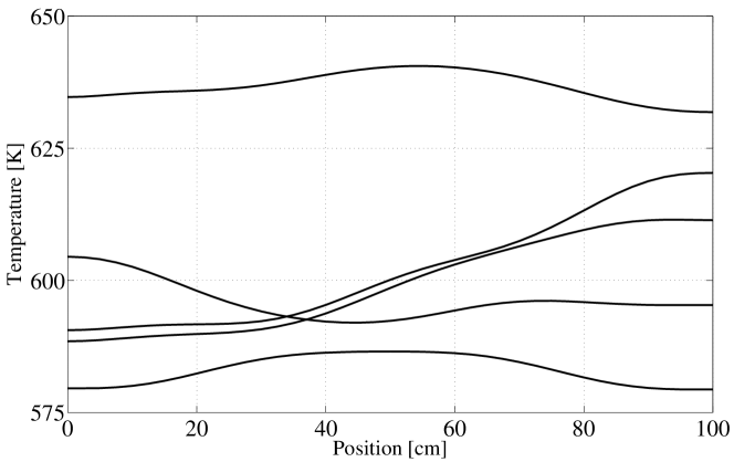
Refer to caption
(a) Temperature.
Refer to caption
(b) Neutron flux.
Figure 4: Monte Carlo simulation: five samples of the solution.

First, we carried out a Monte Carlo simulation. We generated MC=100,000𝑀𝐶100000MC=100,000 pairs of sample paths of the thermal transmittance and absorption cross section random fields. Then, for each pair of sample paths, we constructed the associated deterministic multiphysics model. We solved each model by using the FE method for spatial discretization and Gauss-Seidel iteration. We systematically obtained converged results for 404040 finite elements and 202020 iterations.

Figure 4 shows a few samples of the random temperature and neutron flux thus obtained. The samples of the random temperature (Fig. 4(a)) are smoother than those of the thermal transmittance random field (Fig. 2(a)), that is, the former samples exhibit less rapid oscillations with respect to the position in the reactor than the latter samples. In [11], we had shown that this behavior can be attributed to the large magnitude of the diffusion term of the heat subproblem, which reduces the nonuniformity of the samples of the random temperature.

6.2 PC-based implementation involving dimension reduction and measure transformation

Next, we implemented the proposed polynomial-chaos-based iterative method involving dimension reduction and measure transformation. This implementation corresponded exactly to Algorithm 1. We obtained results by setting the total degree p𝑝p of the chaos expansion of the random temperature to 444 and, with reference to (71) and (72), by using a range of values for the error tolerance levels ϵ1subscriptitalic-ϵ1\epsilon_{1} and ϵ2subscriptitalic-ϵ2\epsilon_{2} to determine the reduced dimension and the total degree of the chaos expansion of the random neutron flux at each iteration. We discuss the convergence of the results as a function of these error tolerance levels later. Now, we present detailed results obtained for ϵ1=0.01subscriptitalic-ϵ10.01\epsilon_{1}=0.01 and ϵ2=0.01subscriptitalic-ϵ20.01\epsilon_{2}=0.01.

Refer to caption

1MCk=1MC𝑻^(𝝃k,𝜻k),p𝑻^(𝝃k,𝜻k)1,p𝑾2/1MCk=1MC𝑻(𝝃k,𝜻k)𝑾2\small{\ell\mapsto\sqrt{\frac{1}{MC}\sum_{k=1}^{MC}\|\widehat{\boldsymbol{T}}{}^{\ell,p}(\boldsymbol{\xi}_{k},\boldsymbol{\zeta}_{k})-\widehat{\boldsymbol{T}}{}^{\ell-1,p}(\boldsymbol{\xi}_{k},\boldsymbol{\zeta}_{k})\|_{\boldsymbol{W}}^{2}}\Big{/}\sqrt{\frac{1}{MC}\sum_{k=1}^{MC}\|{\boldsymbol{T}}{}^{\infty}(\boldsymbol{\xi}_{k},\boldsymbol{\zeta}_{k})\|_{\boldsymbol{W}}^{2}}}\normalsize (circles).

1MCk=1MC𝚽^(𝜼,p(𝝃k),𝜻k),q𝚽^(𝜼1,p(𝝃k),𝜻k)1,q𝑾2/1MCk=1MC𝚽(𝝃k,𝜻k)𝑾2\small{\ell\mapsto\sqrt{\frac{1}{MC}\sum_{k=1}^{MC}\|\widehat{\boldsymbol{\Phi}}{}^{\ell,q}(\boldsymbol{\eta}^{\ell,p}(\boldsymbol{\xi}_{k}),\boldsymbol{\zeta}_{k})-\widehat{\boldsymbol{\Phi}}{}^{\ell-1,q}(\boldsymbol{\eta}^{\ell-1,p}(\boldsymbol{\xi}_{k}),\boldsymbol{\zeta}_{k})\|_{\boldsymbol{W}}^{2}}\Big{/}\sqrt{\frac{1}{MC}\sum_{k=1}^{MC}\|{\boldsymbol{\Phi}}{}^{\infty}(\boldsymbol{\xi}_{k},\boldsymbol{\zeta}_{k})\|_{\boldsymbol{W}}^{2}}}\normalsize (squares).

Figure 5: PC-based simulation: convergence with respect to the number of iterations.
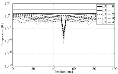
Figure 5 shows the convergence of the iterative method as a function of the number of iterations; note that the superscript \infty is used in the figure captions to indicate convergence with respect to the number of iterations. The iterative method converged linearly up to approximately iteration =77\ell=7, after which linear-solver tolerances became dominant and prevented further convergence. All results to follow were obtained at iteration =2020\ell=20 and can thus be considered to have converged with respect to the number of iterations.
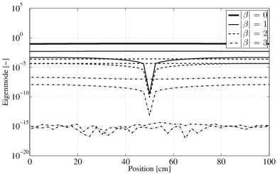
Refer to caption
(a) Mean (thick solid) and first (thin solid), second (dashed), third (dash-dotted), and fourth (dotted) order coefficients 𝑻¯𝜷\overline{\boldsymbol{T}}{}^{\infty}_{\boldsymbol{\beta}} of the chaos expansion 𝑻¯(𝜻),p=|𝜷|=0p𝑻¯ψ𝜷𝜷(𝜻)\overline{\boldsymbol{T}}{}^{\infty,p}(\boldsymbol{\zeta})=\sum_{|\boldsymbol{\beta}|=0}^{p}\overline{\boldsymbol{T}}{}^{\infty}_{\boldsymbol{\beta}}\psi_{\boldsymbol{\beta}}(\boldsymbol{\zeta}).
Refer to caption
(b) Eigenvalues {λj,1j10}superscriptsubscript𝜆𝑗1𝑗10\{\lambda_{j}^{\infty},1\leq j\leq 10\}.
Refer to caption
(c) Mean (thick solid) and first (thin solid), second (dashed), and third (dash-dotted) order coefficients ϕ𝜷1,subscriptsuperscriptbold-italic-ϕ1𝜷\boldsymbol{\phi}^{1,\infty}_{\boldsymbol{\beta}} of the chaos expansion ϕ1,,p1(𝜻)=|𝜷|=0p1ϕ𝜷1,ψ𝜷(𝜻)superscriptbold-italic-ϕ1𝑝1𝜻superscriptsubscript𝜷0𝑝1subscriptsuperscriptbold-italic-ϕ1𝜷subscript𝜓𝜷𝜻\boldsymbol{\phi}^{1,\infty,p-1}(\boldsymbol{\zeta})=\sum_{|\boldsymbol{\beta}|=0}^{p-1}\boldsymbol{\phi}^{1,\infty}_{\boldsymbol{\beta}}\psi_{\boldsymbol{\beta}}(\boldsymbol{\zeta}).
Refer to caption
(d) Mean (thick solid) and first (thin solid), second (dashed), and third (dash-dotted) order coefficients ϕ𝜷2,subscriptsuperscriptbold-italic-ϕ2𝜷\boldsymbol{\phi}^{2,\infty}_{\boldsymbol{\beta}} of the chaos expansion ϕ2,,p1(𝜻)=|𝜷|=0p1ϕ𝜷2,ψ𝜷(𝜻)superscriptbold-italic-ϕ2𝑝1𝜻superscriptsubscript𝜷0𝑝1subscriptsuperscriptbold-italic-ϕ2𝜷subscript𝜓𝜷𝜻\boldsymbol{\phi}^{2,\infty,p-1}(\boldsymbol{\zeta})=\sum_{|\boldsymbol{\beta}|=0}^{p-1}\boldsymbol{\phi}^{2,\infty}_{\boldsymbol{\beta}}\psi_{\boldsymbol{\beta}}(\boldsymbol{\zeta}).
Refer to caption
(e) Coefficients η1,𝜶subscriptsuperscript𝜂1𝜶\eta^{\infty}_{1,\boldsymbol{\alpha}} of the chaos expansion η1,p(𝝃)=|𝜶|=1pη1,𝜶φ𝜶(𝝃)subscriptsuperscript𝜂𝑝1𝝃superscriptsubscript𝜶1𝑝subscriptsuperscript𝜂1𝜶subscript𝜑𝜶𝝃\eta^{\infty,p}_{1}(\boldsymbol{\xi})=\sum_{|\boldsymbol{\alpha}|=1}^{p}\eta^{\infty}_{1,\boldsymbol{\alpha}}\varphi_{\boldsymbol{\alpha}}(\boldsymbol{\xi}).
Refer to caption
(f) Coefficients η2,𝜶subscriptsuperscript𝜂2𝜶\eta^{\infty}_{2,\boldsymbol{\alpha}} of the chaos expansion η2,p(𝝃)=|𝜶|=1pη2,𝜶φ𝜶(𝝃)subscriptsuperscript𝜂𝑝2𝝃superscriptsubscript𝜶1𝑝subscriptsuperscript𝜂2𝜶subscript𝜑𝜶𝝃\eta^{\infty,p}_{2}(\boldsymbol{\xi})=\sum_{|\boldsymbol{\alpha}|=1}^{p}\eta^{\infty}_{2,\boldsymbol{\alpha}}\varphi_{\boldsymbol{\alpha}}(\boldsymbol{\xi}).
Figure 6: PC-based simulation: a few components of the reduced chaos expansion with random coefficients, 𝑻^(𝝃,𝜻),p,d=𝑻¯(𝜻),p+j=1dλjηj,p(𝝃)ϕj,,p1(𝜻)\widehat{\boldsymbol{T}}{}^{\infty,p,d}(\boldsymbol{\xi},\boldsymbol{\zeta})=\overline{\boldsymbol{T}}{}^{\infty,p}(\boldsymbol{\zeta})+\sum_{j=1}^{d}\sqrt{\lambda_{j}^{\infty}}\,\eta_{j}^{\infty,p}(\boldsymbol{\xi})\,\boldsymbol{\phi}^{j,\infty,p-1}(\boldsymbol{\zeta}), of the random temperature.
Refer to caption
(a) Joint probability density function.
Refer to caption
(b) First marginal probability density function.
Refer to caption
(c) Second marginal probability density function.
Figure 7: PC-based simulation: probability distribution of the first and second reduced random variables of the reduced chaos expansion with random coefficients of the random temperature.

Figure 6 shows a few components of the reduced chaos expansion with random coefficients of the random temperature. We can observe that the eigenvalues of the reduced chaos expansion with random coefficients of the random temperature (Fig. 6(b)) decay at a higher rate than those of the KL decomposition of the thermal transmittance random field (Fig. 2(b)). This result is consistent with our earlier observation that the samples of the random temperature are smoother than those of the thermal transmittance random field.

Figure 7 shows the joint and marginal probability density functions of the reduced random variables. Clearly, the joint probability density function shows statistical dependence, and the marginal probability density functions are not “labeled.”

At iteration =2020\ell=20, a reduced chaos expansion with random coefficients obtained by retaining only d=2𝑑2d=2 terms was found to be sufficiently accurate to satisfy (71) for ϵ1=0.01subscriptitalic-ϵ10.01\epsilon_{1}=0.01; thus, at this iteration, the measure transformation necessitated the construction of polynomial chaos and quadrature rules with respect to the joint probability distribution of the reduced random variables 𝜼,p=(η1,p,η2,p)superscript𝜼𝑝subscriptsuperscript𝜂𝑝1subscriptsuperscript𝜂𝑝2\boldsymbol{\eta}^{\ell,p}=(\eta^{\ell,p}_{1},\eta^{\ell,p}_{2}) and the input random variables 𝜻=(ζ1,ζ2)𝜻subscript𝜁1subscript𝜁2\boldsymbol{\zeta}=(\zeta_{1},\zeta_{2}).

Refer to caption
(a) Γ00superscriptsubscriptΓ00\Gamma_{00}^{\infty}.
Refer to caption
(b) Γ10superscriptsubscriptΓ10\Gamma_{10}^{\infty}.
Refer to caption
(c) Γ01superscriptsubscriptΓ01\Gamma_{01}^{\infty}.
Refer to caption
(d) Γ20superscriptsubscriptΓ20\Gamma_{20}^{\infty}.
Refer to caption
(e) Γ11superscriptsubscriptΓ11\Gamma_{11}^{\infty}.
Refer to caption
(f) Γ02superscriptsubscriptΓ02\Gamma_{02}^{\infty}.
Figure 8: PC-based simulation: computed polynomial chaos up to a total degree q𝑞q of 222.

Figure 8 illustrates the proposed computational construction of polynomial chaos with respect to P𝜼subscriptsuperscript𝑃𝜼P^{\ell}_{\boldsymbol{\eta}}; specifically, the figure shows the polynomial chaos obtained up to a total degree q𝑞q of 222. With reference to Sec. 5.8, the requisite polynomial chaos with respect to P𝜼×P𝜻superscriptsubscript𝑃𝜼subscript𝑃𝜻P_{\boldsymbol{\eta}}^{\ell}\times P_{\boldsymbol{\zeta}} are synthesized from the computed polynomial chaos thus obtained with respect to P𝜼subscriptsuperscript𝑃𝜼P^{\ell}_{\boldsymbol{\eta}} and the normalized Legendre polynomials with respect to P𝜻subscript𝑃𝜻P_{\boldsymbol{\zeta}} by tensorization.

Refer to caption
(a) {𝜼k,λ,1kνλ}superscriptsubscript𝜼𝑘𝜆1𝑘subscriptsuperscript𝜈𝜆\{\boldsymbol{\eta}_{k}^{\infty,\lambda},1\leq k\leq\nu^{\infty}_{\lambda}\} for λ=1𝜆1\lambda=1.
Refer to caption
(b) {wk,λ,1kνλ}superscriptsubscript𝑤𝑘𝜆1𝑘subscriptsuperscript𝜈𝜆\{w_{k}^{\infty,\lambda},1\leq k\leq\nu^{\infty}_{\lambda}\} for λ=1𝜆1\lambda=1.
Refer to caption
(c) {𝜼k,λ,1kνλ}superscriptsubscript𝜼𝑘𝜆1𝑘subscriptsuperscript𝜈𝜆\{\boldsymbol{\eta}_{k}^{\infty,\lambda},1\leq k\leq\nu^{\infty}_{\lambda}\} for λ=2𝜆2\lambda=2.
Refer to caption
(d) {wk,λ,1kνλ}superscriptsubscript𝑤𝑘𝜆1𝑘subscriptsuperscript𝜈𝜆\{w_{k}^{\infty,\lambda},1\leq k\leq\nu^{\infty}_{\lambda}\} for λ=2𝜆2\lambda=2.
Refer to caption
(e) {𝜼k,λ,1kνλ}superscriptsubscript𝜼𝑘𝜆1𝑘subscriptsuperscript𝜈𝜆\{\boldsymbol{\eta}_{k}^{\infty,\lambda},1\leq k\leq\nu^{\infty}_{\lambda}\} for λ=3𝜆3\lambda=3.
Refer to caption
(f) {wk,λ,1kνλ}superscriptsubscript𝑤𝑘𝜆1𝑘subscriptsuperscript𝜈𝜆\{w_{k}^{\infty,\lambda},1\leq k\leq\nu^{\infty}_{\lambda}\} for λ=3𝜆3\lambda=3.
Refer to caption
(g) {𝜼k,λ,1kνλ}superscriptsubscript𝜼𝑘𝜆1𝑘subscriptsuperscript𝜈𝜆\{\boldsymbol{\eta}_{k}^{\infty,\lambda},1\leq k\leq\nu^{\infty}_{\lambda}\} for λ=4𝜆4\lambda=4.
Refer to caption
(h) {wk,λ,1kνλ}superscriptsubscript𝑤𝑘𝜆1𝑘subscriptsuperscript𝜈𝜆\{w_{k}^{\infty,\lambda},1\leq k\leq\nu^{\infty}_{\lambda}\} for λ=4𝜆4\lambda=4.
Figure 9: PC-based simulation: computed quadrature rules up to a level λ𝜆\lambda of 444.

Figure 9 illustrates the proposed computational construction of quadrature rules with respect to P𝜼subscriptsuperscript𝑃𝜼P^{\ell}_{\boldsymbol{\eta}}; specifically, the figure shows the quadrature rules obtained up to a level λ𝜆\lambda of 444. This figure indicates that as λ𝜆\lambda was increased, higher accuracy was required, and thus, a quadrature rule with more nodes and weights was systematically obtained. With reference to Sec. 5.8, the requisite quadrature rules with respect to P𝜼×P𝜻superscriptsubscript𝑃𝜼subscript𝑃𝜻P_{\boldsymbol{\eta}}^{\ell}\times P_{\boldsymbol{\zeta}} are synthesized from the computed quadrature rules obtained with respect to P𝜼subscriptsuperscript𝑃𝜼P^{\ell}_{\boldsymbol{\eta}} and the fully tensorized Gauss-Legendre quadrature rules with respect to P𝜻subscript𝑃𝜻P_{\boldsymbol{\zeta}} by tensorization.

Refer to caption
(a) Coefficients 𝑻^𝜶𝜷\widehat{\boldsymbol{T}}{}^{\infty}_{\boldsymbol{\alpha}\boldsymbol{\beta}} indexed by multi-indices (𝜶,𝜷)𝜶𝜷(\boldsymbol{\alpha},\boldsymbol{\beta}) with |𝜷|=0𝜷0|\boldsymbol{\beta}|=0 (thick circles), |𝜷|=1𝜷1|\boldsymbol{\beta}|=1 (thin circles), |𝜷|=2𝜷2|\boldsymbol{\beta}|=2 (squares), |𝜷|=3𝜷3|\boldsymbol{\beta}|=3 (diamonds), and |𝜷|=4𝜷4|\boldsymbol{\beta}|=4 (pentagrams) of the chaos expansion 𝑻^(𝝃,𝜻),p=|𝜶|+|𝜷|=0p𝑻^φ𝜶𝜶𝜷(𝝃)ψ𝜷(𝜻)\widehat{\boldsymbol{T}}{}^{\infty,p}(\boldsymbol{\xi},\boldsymbol{\zeta})=\sum_{|\boldsymbol{\alpha}|+|\boldsymbol{\beta}|=0}^{p}\widehat{\boldsymbol{T}}{}^{\infty}_{\boldsymbol{\alpha}\boldsymbol{\beta}}\varphi_{\boldsymbol{\alpha}}(\boldsymbol{\xi})\psi_{\boldsymbol{\beta}}(\boldsymbol{\zeta}) at x=10[cm]𝑥10delimited-[]cmx=10\,\text{$[\text{cm}]$}.
Refer to caption
(b) Coefficients 𝚽^𝜷𝜸\widehat{\boldsymbol{\Phi}}{}^{\infty}_{\boldsymbol{\beta}\boldsymbol{\gamma}} indexed by multi-indices (𝜷,𝜸)𝜷𝜸(\boldsymbol{\beta},\boldsymbol{\gamma}) with |𝜸|=0𝜸0|\boldsymbol{\gamma}|=0 (thick circles), |𝜸|=1𝜸1|\boldsymbol{\gamma}|=1 (thin circles), and |𝜸|=2𝜸2|\boldsymbol{\gamma}|=2 (squares) of the chaos expansion 𝚽^(𝜼,p,𝜻),q=|𝜸|+|𝜷|=0q𝚽^Γ𝜸𝜸𝜷(𝜼,p)ψ𝜷(𝜻)\widehat{\boldsymbol{\Phi}}{}^{\infty,q}(\boldsymbol{\eta}^{\infty,p},\boldsymbol{\zeta})=\sum_{|\boldsymbol{\gamma}|+|\boldsymbol{\beta}|=0}^{q}\widehat{\boldsymbol{\Phi}}{}^{\infty}_{\boldsymbol{\gamma}\boldsymbol{\beta}}\Gamma_{\boldsymbol{\gamma}}^{\infty}(\boldsymbol{\eta}^{\infty,p})\psi_{\boldsymbol{\beta}}(\boldsymbol{\zeta}) at x=10[cm]𝑥10delimited-[]cmx=10\,\text{$[\text{cm}]$}.
Figure 10: PC-based simulation: coefficients of the solution at x=10[cm]𝑥10delimited-[]cmx=10\,\text{$[\text{cm}]$}.

At iteration =2020\ell=20, a chaos expansion truncated at q=2𝑞2q=2 was found to be sufficiently accurate to satisfy (72) for ϵ2=0.01subscriptitalic-ϵ20.01\epsilon_{2}=0.01. The representation of the random temperature by a chaos expansion of dimension m+n=12𝑚𝑛12m+n=12 and total degree p=4𝑝4p=4 requires 1,820=16!/12!/4!1820161241,820=16!/12!/4! terms; in contrast, the representation of the random neutron flux by a chaos expansion of dimension d+n=4𝑑𝑛4d+n=4 and total degree q=2𝑞2q=2 requires only 15=6!/4!/2!1564215=6!/4!/2! terms. The sparse-grid Gauss-Legendre quadrature rule of dimension m+n=12𝑚𝑛12m+n=12 and level p+1=5𝑝15p+1=5 used to compute the coefficients of the chaos expansion of the random temperature has 34,0653406534,065 nodes and weights; in contrast, the sparse-grid quadrature rule of dimension d+n=4𝑑𝑛4d+n=4 and level q+2=4𝑞24q+2=4 used to compute the coefficients of the chaos expansion of the random neutron flux has only 346346346 nodes and weights. Figure 10 shows a few coefficients of the solution.
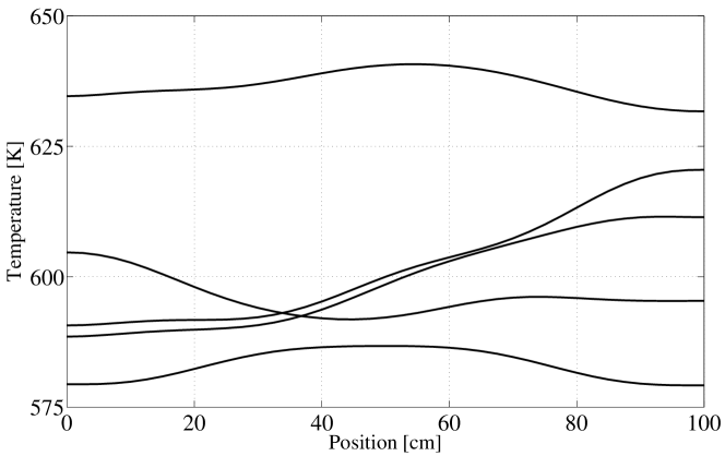
Refer to caption
(a) Temperature.
Refer to caption
(b) Neutron flux.
Figure 11: PC-based simulation: five samples of the solution.

Figure 11 shows a few samples of the random temperature and random neutron flux deduced from the chaos expansions obtained as the output of the solution algorithm. The samples of the input random variables used to synthesize the samples of the random temperature and random neutron flux shown in Fig. 11 were identical to those used to generate the samples shown in Fig. 4. The similarity of the samples in Figs. 4 and 11 indicates that the surrogate model based on polynomial chaos not only provides an accurate global representation of the multiphysics model but is also capable of accurately reproducing a sample-wise response.

6.3 Sensitivity analysis of the random temperature and random neutron flux

The chaos expansions in (70) facilitate the following decompositions of the variances of the random temperature and random neutron flux:

VTsuperscript𝑉𝑇\displaystyle V^{T} =V𝝃T+V𝜻T+V(𝝃,𝜻)T,absentsubscriptsuperscript𝑉𝑇𝝃subscriptsuperscript𝑉𝑇𝜻subscriptsuperscript𝑉𝑇𝝃𝜻\displaystyle=V^{T}_{\boldsymbol{\xi}}+V^{T}_{\boldsymbol{\zeta}}+V^{T}_{(\boldsymbol{\xi},\boldsymbol{\zeta})}, VΦsuperscript𝑉Φ\displaystyle V^{\Phi} =V𝝃Φ+V𝜻Φ+V(𝝃,𝜻)Φ,absentsubscriptsuperscript𝑉Φ𝝃subscriptsuperscript𝑉Φ𝜻subscriptsuperscript𝑉Φ𝝃𝜻\displaystyle=V^{\Phi}_{\boldsymbol{\xi}}+V^{\Phi}_{\boldsymbol{\zeta}}+V^{\Phi}_{(\boldsymbol{\xi},\boldsymbol{\zeta})}, (73)
VTsuperscript𝑉𝑇\displaystyle V^{T} =|𝜶|+|𝜷|=1pT^𝑾2𝜶𝜷,\displaystyle=\sum_{|\boldsymbol{\alpha}|+|\boldsymbol{\beta}|=1}^{p}\|\widehat{T}{}^{\infty}_{\boldsymbol{\alpha}\boldsymbol{\beta}}\|_{\boldsymbol{W}}^{2}, VΦsuperscript𝑉Φ\displaystyle V^{\Phi} =|𝜸|+|𝜷|=1qΦ^𝑾2𝜸𝜷,\displaystyle=\sum_{|\boldsymbol{\gamma}|+|\boldsymbol{\beta}|=1}^{q}\|\widehat{\Phi}{}^{\infty}_{\boldsymbol{\gamma}\boldsymbol{\beta}}\|_{\boldsymbol{W}}^{2},
V𝝃Tsuperscriptsubscript𝑉𝝃𝑇\displaystyle V_{\boldsymbol{\xi}}^{T} =|𝜶|=1pT^𝑾2𝜶𝟎,\displaystyle=\sum_{\;\;\;\,|\boldsymbol{\alpha}|=1\;\;\;\,}^{p}\|\widehat{T}{}^{\infty}_{\boldsymbol{\alpha}\boldsymbol{0}}\|_{\boldsymbol{W}}^{2}, V𝝃Φsuperscriptsubscript𝑉𝝃Φ\displaystyle V_{\boldsymbol{\xi}}^{\Phi} =|𝜸|=1qΦ^𝑾2𝜸𝟎,\displaystyle=\sum_{\;\;\;\,|\boldsymbol{\gamma}|=1\;\;\;\,}^{q}\|\widehat{\Phi}{}^{\infty}_{\boldsymbol{\gamma}\boldsymbol{0}}\|_{\boldsymbol{W}}^{2},
V𝜻Tsuperscriptsubscript𝑉𝜻𝑇\displaystyle V_{\boldsymbol{\zeta}}^{T} =|𝜷|=1pT^𝑾2𝟎𝜷,\displaystyle=\sum_{\;\;\;\,|\boldsymbol{\beta}|=1\;\;\;\,}^{p}\|\widehat{T}{}^{\infty}_{\boldsymbol{0}\boldsymbol{\beta}}\|_{\boldsymbol{W}}^{2}, V𝜻Φsuperscriptsubscript𝑉𝜻Φ\displaystyle V_{\boldsymbol{\zeta}}^{\Phi} =|𝜷|=1qΦ^𝑾2𝟎𝜷,\displaystyle=\sum_{\;\;\;\,|\boldsymbol{\beta}|=1\;\;\;\,}^{q}\|\widehat{\Phi}{}^{\infty}_{\boldsymbol{0}\boldsymbol{\beta}}\|_{\boldsymbol{W}}^{2},
V(𝝃,𝜻)Tsuperscriptsubscript𝑉𝝃𝜻𝑇\displaystyle V_{(\boldsymbol{\xi},\boldsymbol{\zeta})}^{T} =|𝜶|+|𝜷|=1𝜶𝟎,𝜷𝟎pT^𝑾2𝜶𝜷,\displaystyle=\sum_{\begin{subarray}{c}|\boldsymbol{\alpha}|+|\boldsymbol{\beta}|=1\\ \boldsymbol{\alpha}\neq\boldsymbol{0},\boldsymbol{\beta}\neq\boldsymbol{0}\end{subarray}}^{p}\|\widehat{T}{}^{\infty}_{\boldsymbol{\alpha}\boldsymbol{\beta}}\|_{\boldsymbol{W}}^{2}, V(𝝃,𝜻)Φsuperscriptsubscript𝑉𝝃𝜻Φ\displaystyle V_{(\boldsymbol{\xi},\boldsymbol{\zeta})}^{\Phi} =|𝜸|+|𝜷|=1𝜸𝟎,𝜷𝟎qΦ^𝑾2𝜸𝜷.\displaystyle=\sum_{\begin{subarray}{c}|\boldsymbol{\gamma}|+|\boldsymbol{\beta}|=1\\ \boldsymbol{\gamma}\neq\boldsymbol{0},\boldsymbol{\beta}\neq\boldsymbol{0}\end{subarray}}^{q}\|\widehat{\Phi}{}^{\infty}_{\boldsymbol{\gamma}\boldsymbol{\beta}}\|_{\boldsymbol{W}}^{2}.

Here, V𝝃Tsuperscriptsubscript𝑉𝝃𝑇V_{\boldsymbol{\xi}}^{T} and V𝝃Φsuperscriptsubscript𝑉𝝃ΦV_{\boldsymbol{\xi}}^{\Phi} are the sums of the variances of those terms in the chaos expansions of the random temperature and random neutron flux, respectively, which depend only on the input random variables 𝝃𝝃\boldsymbol{\xi} that describe the uncertainty in the parameters of the heat subproblem; hence, following the approach given in [22, 23, 24], V𝝃Tsuperscriptsubscript𝑉𝝃𝑇V_{\boldsymbol{\xi}}^{T} and V𝝃Φsuperscriptsubscript𝑉𝝃ΦV_{\boldsymbol{\xi}}^{\Phi} can be interpreted as the portions contributed by the uncertainty in the parameters of the heat subproblem to the variances of the random temperature and random neutron flux, respectively. Conversely, V𝜻Tsuperscriptsubscript𝑉𝜻𝑇V_{\boldsymbol{\zeta}}^{T} and V𝜻Φsuperscriptsubscript𝑉𝜻ΦV_{\boldsymbol{\zeta}}^{\Phi} are the sums of the variances of those terms in the chaos expansions of the random temperature and random neutron flux which depend only on the input random variables 𝜻𝜻\boldsymbol{\zeta} that describe the uncertainty in the parameters of the neutronics subproblem, and they can be interpreted as the portions contributed by the uncertainty in the parameters of the neutronics subproblem to the variances of the random temperature and random neutron flux, respectively. Lastly, V(𝝃,𝜻)Tsuperscriptsubscript𝑉𝝃𝜻𝑇V_{(\boldsymbol{\xi},\boldsymbol{\zeta})}^{T} and V(𝝃,𝜻)Φsuperscriptsubscript𝑉𝝃𝜻ΦV_{(\boldsymbol{\xi},\boldsymbol{\zeta})}^{\Phi} are the portions contributed by the interaction of the uncertainties in the parameters of the heat subproblem and those in the parameters of the neutronics subproblem to the variances of the random temperature and random neutron flux, respectively.

temperature neutron flux
main effect of uncertainty in data of heat subproblem V𝝃TVT=55.45%subscriptsuperscript𝑉𝑇𝝃superscript𝑉𝑇percent55.45\frac{V^{T}_{\boldsymbol{\xi}}}{V^{T}}=55.45\% V𝝃ΦVΦ=2.15%subscriptsuperscript𝑉Φ𝝃superscript𝑉Φpercent2.15\frac{V^{\Phi}_{\boldsymbol{\xi}}}{V^{\Phi}}=2.15\%
main effect of uncertainty in data of neutronics subproblem V𝜻TVT=44.40%subscriptsuperscript𝑉𝑇𝜻superscript𝑉𝑇percent44.40\frac{V^{T}_{\boldsymbol{\zeta}}}{V^{T}}=44.40\% V𝜻ΦVΦ=97.83%subscriptsuperscript𝑉Φ𝜻superscript𝑉Φpercent97.83\frac{V^{\Phi}_{\boldsymbol{\zeta}}}{V^{\Phi}}=97.83\%
interaction of uncertainty in data of heat subproblem and uncertainty in data of neutronics subproblem V(𝝃,𝜻)TVT=0.02%subscriptsuperscript𝑉𝑇𝝃𝜻superscript𝑉𝑇percent0.02\frac{V^{T}_{(\boldsymbol{\xi},\boldsymbol{\zeta})}}{V^{T}}=0.02\% V(𝝃,𝜻)ΦVΦ=0.08%subscriptsuperscript𝑉Φ𝝃𝜻superscript𝑉Φpercent0.08\frac{V^{\Phi}_{(\boldsymbol{\xi},\boldsymbol{\zeta})}}{V^{\Phi}}=0.08\%
Table 1: Decomposition of the variances of the random temperature and random neutron flux.

We obtained the values given in Table 1; these values indicate that the uncertainty in the parameters of the heat subproblem predominantly drives the uncertainty in the temperature (55.45%percent55.4555.45\%) and that the uncertainty in the parameters of the neutronics subproblem predominantly drives the uncertainty in the neutron flux (97.83%percent97.8397.83\%). Further, we can observe that the uncertainty in the parameters of the heat subproblem is less important in driving the uncertainty in the neutron flux than the uncertainty in the parameters of the neutronics subproblem is in driving the uncertainty in the temperature (2.15%percent2.152.15\% versus 44.40%percent44.4044.40\%). This observation can be explained as a consequence of the coupling mechanism adopted in this work; with reference to (47), this coupling mechanism involves the division of the temperature by a large reference temperature as it feeds into the coefficients of the neutronics subproblem, thus diminishing the impact that fluctuations in the temperature have on the neutron flux.

6.4 Convergence analysis
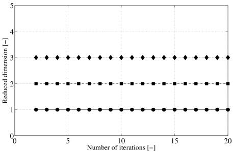
Refer to caption
(a) Reduced dimension d𝑑d.
Refer to caption
(b) 1MCk=1MC𝑻(𝝃k,𝜻k)𝑻^(𝝃k,𝜻k),p𝑾2/1MCk=1MC𝑻(𝝃k,𝜻k)𝑾2\ell\mapsto\sqrt{\frac{1}{MC}\sum_{k=1}^{MC}\|\boldsymbol{T}^{\ell}(\boldsymbol{\xi}_{k},\boldsymbol{\zeta}_{k})-\widehat{\boldsymbol{T}}{}^{\ell,p}(\boldsymbol{\xi}_{k},\boldsymbol{\zeta}_{k})\|_{\boldsymbol{W}}^{2}}\Big{/}\sqrt{\frac{1}{MC}\sum_{k=1}^{MC}\|\boldsymbol{T}^{\infty}(\boldsymbol{\xi}_{k},\boldsymbol{\zeta}_{k})\|_{\boldsymbol{W}}^{2}}.
Refer to caption
(c) 1MCk=1MC𝚽(𝝃k,𝜻k)𝚽^(𝜼,p(𝝃k),𝜻k),q𝑾2/1MCk=1MC𝚽(𝝃k,𝜻k)𝑾2\ell\mapsto\sqrt{\frac{1}{MC}\sum_{k=1}^{MC}\|\boldsymbol{\Phi}^{\ell}(\boldsymbol{\xi}_{k},\boldsymbol{\zeta}_{k})-\widehat{\boldsymbol{\Phi}}{}^{\ell,q}(\boldsymbol{\eta}^{\ell,p}(\boldsymbol{\xi}_{k}),\boldsymbol{\zeta}_{k})\|_{\boldsymbol{W}}^{2}}\Big{/}\sqrt{\frac{1}{MC}\sum_{k=1}^{MC}\|\boldsymbol{\Phi}^{\infty}(\boldsymbol{\xi}_{k},\boldsymbol{\zeta}_{k})\|_{\boldsymbol{W}}^{2}}.
Figure 12: Convergence analysis: (a) reduced dimension and (b, c) mean-square distance between the successive approximations determined by the simulation based on Monte Carlo sampling and the simulation based on polynomial chaos for ϵ1=0.02subscriptitalic-ϵ10.02\epsilon_{1}=0.02 (circles), ϵ1=0.01subscriptitalic-ϵ10.01\epsilon_{1}=0.01 (squares), and ϵ1=0.005subscriptitalic-ϵ10.005\epsilon_{1}=0.005 (diamonds) and ϵ2=0.01subscriptitalic-ϵ20.01\epsilon_{2}=0.01 as a function of the number of iterations.
Refer to caption
(a) Total degree q𝑞q.
Refer to caption
(b) 1MCk=1MC𝑻(𝝃k,𝜻k)𝑻^(𝝃k,𝜻k),p𝑾2/1MCk=1MC𝑻(𝝃k,𝜻k)𝑾2\ell\mapsto\sqrt{\frac{1}{MC}\sum_{k=1}^{MC}\|\boldsymbol{T}^{\ell}(\boldsymbol{\xi}_{k},\boldsymbol{\zeta}_{k})-\widehat{\boldsymbol{T}}{}^{\ell,p}(\boldsymbol{\xi}_{k},\boldsymbol{\zeta}_{k})\|_{\boldsymbol{W}}^{2}}\Big{/}\sqrt{\frac{1}{MC}\sum_{k=1}^{MC}\|\boldsymbol{T}^{\infty}(\boldsymbol{\xi}_{k},\boldsymbol{\zeta}_{k})\|_{\boldsymbol{W}}^{2}}.
Refer to caption
(c) 1MCk=1MC𝚽(𝝃k,𝜻k)𝚽^(𝜼,p(𝝃k),𝜻k),q𝑾2/1MCk=1MC𝚽(𝝃k,𝜻k)𝑾2\ell\mapsto\sqrt{\frac{1}{MC}\sum_{k=1}^{MC}\|\boldsymbol{\Phi}^{\ell}(\boldsymbol{\xi}_{k},\boldsymbol{\zeta}_{k})-\widehat{\boldsymbol{\Phi}}{}^{\ell,q}(\boldsymbol{\eta}^{\ell,p}(\boldsymbol{\xi}_{k}),\boldsymbol{\zeta}_{k})\|_{\boldsymbol{W}}^{2}}\Big{/}\sqrt{\frac{1}{MC}\sum_{k=1}^{MC}\|\boldsymbol{\Phi}^{\infty}(\boldsymbol{\xi}_{k},\boldsymbol{\zeta}_{k})\|_{\boldsymbol{W}}^{2}}.
Figure 13: Convergence analysis: (a) total degree and (b,c) mean-square distance between the successive approximations determined by the simulation based on Monte Carlo sampling and the simulation based on polynomial chaos for ϵ1=0.01subscriptitalic-ϵ10.01\epsilon_{1}=0.01 and ϵ2=0.1subscriptitalic-ϵ20.1\epsilon_{2}=0.1 (circles), ϵ2=0.01subscriptitalic-ϵ20.01\epsilon_{2}=0.01 (squares), and ϵ2=0.001subscriptitalic-ϵ20.001\epsilon_{2}=0.001 (diamonds) as a function of the number of iterations.

We repeated the simulation based on polynomial chaos for several values of the error tolerance levels. Each error tolerance level corresponded to a specific accuracy that the reduced chaos expansion with random coefficients of the random temperature and the chaos expansion of the random neutron flux were required to maintain at each iteration. Figures 12(a) and 13(a) indicate that more terms were retained in these expansions when higher accuracy was required.

Further, Figs. 12 ((b) and (c)) and 13 ((b) and (c)) indicate that the distance between the successive approximations determined by the simulation based on Monte Carlo sampling and the simulation based on polynomial chaos remained bounded as the iterations progressed and that this distance can be reduced systematically by improving the accuracy of the reduced chaos expansion with random coefficients of the random temperature and the chaos expansion of the random neutron flux by decreasing the respective error tolerance levels.

6.5 Concluding remarks

The proposed methodology provided the solution of the neutronics subproblem in a reduced-dimensional space because the reduced chaos expansion with random coefficients could facilitate a low-dimensional representation of the random temperature as it passed from the heat subproblem to the neutronics subproblem. While accuracy was maintained, the solution in a reduced-dimensional space resulted in computational gains because of the following two factors. First, the solution in a reduced-dimensional space facilitated the accurate representation of the random neutron flux by a chaos expansion that contained only a few terms. Second, the coefficients in the chaos expansion of the random neutron flux could be computed by using a quadrature rule that had only a few nodes, and thus, the solution of only a few samples of the neutronics subproblem was required at each iteration.

7 Conclusion

We presented a characterization of information by a reduced chaos expansion with random coefficients as this information passes from a subproblem of a stochastic coupled problem to another and from iteration to iteration. This expansion provides a reduced-dimensional representation of the exchanged information, while maintaining segregation between statistically independent sources of uncertainty that stem from different subproblems. Further, we presented a measure transformation that allows stochastic expansion methods to exploit this dimension reduction to obtain an efficient solution of subproblems in a reduced-dimensional space. We showed that owing to the uncertainty source segregation, polynomial chaos and quadrature rules required for the implementation of this measure transformation can be readily obtained by tensorization. The effectiveness of the methodology was demonstrated by considering a multiphysics problem in nuclear engineering.

Acknowledgements

This work was supported by the Department of Energy (DOE) through an Applied Scientific Computing Research (ASCR) grant. The authors would also like to thank Professor Christian Soize for relevant discussions during the final stages of the preparation of this paper.

References

  • Cramér [1999] H. Cramér. Mathematical Methods of Statistics. Princeton University Press, Princeton, New Jersey, 1999.
  • Kullback [1997] S. Kullback. Information Theory and Statistics. Dover Publications, Mineola, New York, 1997.
  • Robert and Casella [2010] C. Robert and G. Casella. Monte Carlo Statistical Methods. Springer, New York, 2010.
  • Ghanem and Spanos [2003] R. Ghanem and P. Spanos. Stochastic Finite Elements: A Spectral Approach. Dover Publications, Mineola, New York, 2003.
  • Soize and Ghanem [2004] C. Soize and R. Ghanem. Physical systems with random uncertainties: Chaos representations with arbitrary probability measure. SIAM Journal on Scientific Computing, 26:395–410, 2004. DOI: 10.1137/S1064827503424505.
  • Ghanem [1998] R. Ghanem. Hybrid stochastic finite elements and generalized Monte Carlo simulation. Journal of Applied Mechanics, 65:1004–1009, 1998. DOI: 10.1115/1.2791894.
  • Ghanem and Ghiocel [1998] R. Ghanem and D. Ghiocel. A new implementation of the spectral stochastic finite element method for stochastic constitutive relations. In ASCE 12th Engineering Mechanics Conference, La Jolla, California, 1998.
  • Ghiocel and Ghanem [2002] D. Ghiocel and R. Ghanem. Stochastic finite-element analysis of seismic soil-structure interaction. ASCE Journal of Engineering Mechanics, 128:66–77, 2002. DOI: 10.1061/(ASCE)0733-9399(2002)128:1(66).
  • Xiu and Hesthaven [2005] D. Xiu and J. Hesthaven. High-order collocation methods for differential equations with random inputs. SIAM Journal on Scientific Computing, 27:1118–1139, 2005. DOI: 10.1137/040615201.
  • Babuska et al. [2007] I. Babuska, F. Nobile, and R. Tempone. A stochastic collocation method for elliptic partial differential equations with random input data. SIAM Journal on Numerical Analysis, 45:1005–1034, 2007. DOI: 10.1137/050645142.
  • Arnst et al. [2011a] M. Arnst, R. Ghanem, E. Phipps, and J. Red Horse. Dimension reduction in stochastic modeling of coupled problems. International Journal for Numerical Methods in Engineering, 2011a. In Press, DOI: 10.1002/nme.4364.
  • Arnst et al. [2011b] M. Arnst, R. Ghanem, E. Phipps, and J. Red Horse. Measure transformation and efficient quadrature in reduced-dimensional stochastic modeling of coupled problems. International Journal for Numerical Methods in Engineering, 2011b. In Press, DOI: 10.1002/nme.4368.
  • Soize and Ghanem [2009] C. Soize and R. Ghanem. Reduced chaos decomposition with random coefficients of vector-valued random variables and random fields. Computer Methods in Applied Mechanics and Engineering, 198:1926–1934, 2009. DOI: 10.1016/j.cma.2008.12.035.
  • Reed and Simon [1980] M. Reed and B. Simon. Methods of Mathematical Physics. Academic Press, San Diego, California, 1980.
  • Stroud and Secrest [2003] A. Stroud and D. Secrest. Gaussian Quadrature Formulas. Prentice-Hall, Englewood Cliffs, New Jersey, 2003.
  • Abramowitz and Stegun [1972] M. Abramowitz and I. Stegun. Handbook of Mathematical Functions: With Formulas, Graphs, and Mathematical Tables. Dover Publications, Mineola, New York, 1972.
  • Xiu and Karniadakis [2003] D. Xiu and G. Karniadakis. Modeling uncertainty in flow simulations via generalized polynomial chaos. Journal of Computational Physics, 187:137–167, 2003. DOI: 10.1016/S0021-9991(03)00092-5.
  • Holtz [2010] M. Holtz. Sparse Grid Quadrature in High Dimensions with Applications in Finance and Insurance. Springer, Berlin, 2010.
  • Bäck et al. [2011] J. Bäck, F. Nobile, L. Tamellini, and R. Tempone. On the optimal polynomial approximation of stochastic PDEs by Galerkin and collocation methods. Technical report, MOX - Polytechnico di Milano, 2011. Submitted for publication.
  • Novak and Ritter [1999] E. Novak and K. Ritter. Simple cubature formulas with high polynomial exactness. Constructive Approximation, 15:499–522, 1999. DOI: 10.1007/s003659900119.
  • Lamarsh [2002] J. Lamarsh. Introduction to Nuclear Reactor Theory. American Nuclear Society, North Kensington, Illinois, 2002.
  • Oakley and O’Hagan [2004] J. Oakley and A. O’Hagan. Probabilistic sensitivity analysis of complex models: A Bayesian approach. Journal of the Royal Statistical Society. Series B, 3:751–769, 2004. DOI: 10.1111/j.1467-9868.2004.05304.x.
  • Sudret [2008] B. Sudret. Global sensitivity analysis using polynomial chaos expansions. Reliability Engineering and System Safety, 93:964–979, 2008. DOI: 10.1016/j.ress.2007.04.002.
  • Crestaux et al. [2009] T. Crestaux, O. Le Maître, and J.-M. Martinez. Polynomial chaos expansion for sensitivity analysis. Reliability Engineering and System Safety, 94:1161–1172, 2009. DOI: 10.1016/j.ress.2008.10.008.