A new look at short-term implied volatility in asset price models with jumps

Abstract.

We analyse the behaviour of the implied volatility smile for options close to expiry in the exponential Lévy class of asset price models with jumps. We introduce a new renormalisation of the strike variable with the property that the implied volatility converges to a non-constant limiting shape, which is a function of both the diffusion component of the process and the jump activity (Blumenthal-Getoor) index of the jump component. Our limiting implied volatility formula relates the jump activity of the underlying asset price process to the short end of the implied volatility surface and sheds new light on the difference between finite and infinite variation jumps from the viewpoint of option prices: in the latter, the wings of the limiting smile are determined by the jump activity indices of the positive and negative jumps, whereas in the former, the wings have a constant model-independent slope. This result gives a theoretical justification for the preference of the infinite variation Lévy models over the finite variation ones in the calibration based on short-maturity option prices.

1. Introduction

In financial markets, the price of a vanilla call or put option on a risky asset with strike $e^{k}$ and maturity $t$ is often quoted in terms of the implied volatility $\widehat{\sigma}(t,k)$ (see (12) in Section 3 for the definition and [10] for more information on implied volatility). Similarly, given a risk-neutral pricing model, one can define a function $(t,k)\mapsto\widehat{\sigma}(t,k)$ via the prices of the vanilla options under that model. The implied volatility is a central object in option markets and it is therefore not surprising that understanding the properties and computing the function $(t,k)\mapsto\widehat{\sigma}(t,k)$ for widely used pricing models has been of considerable interest in the mathematical finance literature. Typically, for a given modelling framework, the implied volatility $\widehat{\sigma}(t,k)$ is not available in closed form. Hence the study of the asymptotic behaviour in a variety of asymptotic regimes (e.g. fixed $t$ and $k\to\pm\infty$ [14, 8, 11]; $t\to\infty$ with $k$ constant [22] or proportional [13] to $t$; $t\to 0$ and $k$ constant [18, 21, 7] etc.) has attracted a lot of attention in the recent years.

In this paper we assume that the returns of the risky asset $S=e^{X}$ are modelled by a Lévy process $X$ and study the relationship between the jump activity of $X$ and the implied volatility at short maturities in the model $S$. Most existing approaches analyse either the at-the-money case, when the implied volatility is determined exclusively by the diffusion component and converges to zero in the pure jump models (see [21, Prop. 5], [15, 12]), or the fixed-strike out-of-the-money case, when the implied volatility for short maturities explodes in the presence of jumps ([17], [7], [21]). However, in the option markets, (a) although the implied volatility for liquid strikes grows with decreasing $t$, it remains within a range of reasonable values and appears not to explode, and (b) the liquid strikes become concentrated around the money as the maturity gets shorter. For instance, in the FX option markets, which are among the most liquid derivatives markets in the world, options with fixed values of the Black-Scholes delta are quoted for each maturity (see [2] for the details on the conventions in FX option markets and a natural parameterisation of the smile using the Black-Scholes delta).

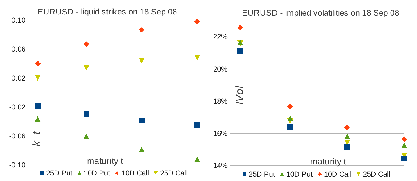
Figure 1. The liquid 10-$\Delta$ and 25-$\Delta$ strikes (left panel) and the corresponding implied volatilities (right panel) for market defined maturities $t\in\{\text{$1$ day, $1$ week, $2$ weeks, $1$ month}\}$ in USDJPY suggest the following: as maturity $t$ becomes small, the relevant strikes $k_{t}$ should approach the at-the-money strike and the implied volatilities $\widehat{\sigma}(t,k_{t})$ should remain bounded.

The market data in Figure 1 therefore suggests that, in order to understand the behaviour of the volatility surface at short maturities, one should look for a moving log-strike $k_{t}\neq 0$, for $t>0$, such that (i) the corresponding implied volatility has a non-trivial limit $\lim_{t\downarrow 0}\widehat{\sigma}(t,k_{t})$ and (ii) the strike $k_{t}$ converges to the at-the-money strike as maturity $t$ tends to zero (i.e. $\lim_{t\downarrow 0}k_{t}=0$).

This paper defines a new universal and model-free parameterisation of the log-strike given by

$$k_{t}=\theta\sqrt{t\log(1/t)}\quad\text{where}\quad\theta\in\mathbb{R}\!\setminus\!\{0\}.$$

For fixed $\theta$, the corresponding strike value tends to the at-the-money strike as $t\downarrow 0$ but is out-of-the-money for each short maturity $t>0$. We prove that under suitable assumptions the limiting implied volatility $\sigma_{0}(\theta)=\lim_{t\downarrow 0}\widehat{\sigma}(t,k_{t})$ takes the following form as a function of $\theta$:

(1) $$\sigma_{0}(\theta)=\max\left\{\frac{-\theta}{\sqrt{1-(\alpha_{-}-1)^{+}}},\sigma,\frac{\theta}{\sqrt{1-(\alpha_{+}-1)^{+}}}\right\}\qquad\text{for any}\qquad\theta\in\mathbb{R}\!\setminus\!\{0\}.$$

In this formula $\sigma$ denotes the volatility of the Gaussian component of the underlying Lévy process $X$ and $\alpha_{+}$ (resp. $\alpha_{-}$) denotes the jump activity (Blumenthal-Getoor) index of the positive (resp. negative) jumps of $X$. More precisely, if the jump measure of $X$ is denoted by $\nu$, $\alpha_{+}$ and $\alpha_{-}$ are given by

$$\alpha_{+}=\inf\{p\geq 0:\int_{(0,1)}|x|^{p}\nu(dx)<\infty\}\quad\text{and}\quad\alpha_{-}=\inf\{p\geq 0:\int_{(-1,0)}|x|^{p}\nu(dx)<\infty\}.$$

Unlike in the case of fixed strike, where short maturity smile explodes in the presence of jumps, our parameterisation of the strike as a function of time yields a non-constant formula for the limiting implied volatility, which depends on the balance between the size of the Gaussian volatility parameter and the activity of small jumps. It allows us to make the following observations about the relationship between the short-dated option prices and the characteristics of the underlying model:

1. the formula for $\sigma_{0}(\theta)$ depends on the jump measure of the log-spot process $X$ only if the jumps are of infinite variation; put differently, if the jumps of $X$ are of finite variation, then the absolute value of the slope of the limiting smile for large $|\theta|$ is equal to one and in particular $\sigma_{0}(\theta)$ does not depend on the structure of jumps;

2. the limiting smile $\sigma_{0}(\theta)$ is V-shaped in the absence of the diffusion component (i.e. when $\sigma=0$) and is U-shaped otherwise;

Remark (i) provides a theoretical basis for distinguishing between the models with jumps of finite and infinite variation in terms of the observed prices of vanilla options with short maturity. It is well-known that, for any short maturity $t$, the market implied smile $k\mapsto\widehat{\sigma}(t,k)$ exhibits pronounced skewness and/or curvature, due, in particular, to the risk of large moves over short time horizons perceived by the investors. Hence, jumps are typically introduced into the risk-neutral pricing models with the aim to capture this risk and modulate the at-the-money skew of the implied volatility $\widehat{\sigma}(t,k)$ at small $t$ (see e.g. [10, Eq (5.10)]). However, since this task can be accomplished by jumps of either finite or infinite variation, this requirement tells us little about the options implied jump activity of the underlying risk-neutral model. On the other hand, the formula for $\sigma_{0}(\theta)$ implies that, if we need to control the tails (in the parameter $\theta$) of the implied volatility for short maturities, we must use jumps of infinite variation. This finding complements the analysis in [6] of the path-wise structure of the risk-neutral process implied by the option prices on the S&P 500 index.

In recent years, there has been a lot of interest in the literature on the statistics of stochastic process in the question of the estimation of the Blumenthal-Getoor index of models with jumps based on high-frequency data. For example, it is shown in [1] that the jump activity (measured by the Blumenthal-Getoor index) estimated on high-frequency stock returns for two large US corporates is well beyond one, implying that the underlying model for stock returns should have jumps of infinite variation. Likewise, the formula in (1) suggests that jumps of infinite variation are needed in order to capture the correct tails (in $\theta$) of the quoted short-dated option prices.

The formula in (1) follows from Corollary 4, which gives the expansion of the implied volatility $\widehat{\sigma}(t,k_{t})$, where $k_{t}=\theta\sqrt{t\log(1/t)}$, up to order $o\left(1/\log(1/t)\right)$. This expansion is consequence of (A) Theorem 3, which itself gives an expansion of the implied volatility for a general log-strike $k_{t}$ that tends to zero as $t\downarrow 0$, and (B) Theorem 1 and Proposition 2, which describe the asymptotic behaviour of the option prices under Lévy processes with infinite and finite jump variations respectively. Theorem 3 relates the asymptotic behaviour of the vanilla option prices under a general semimartingale model to the asymptotic behaviour of the implied volatility as the log-strike $k_{t}$ tends to zero (it should be noted that the asymptotic regime $(t,k_{t})$ in Theorem 3 is not covered by the analysis in [9], see Remark (iv) after Theorem 3 for more details). The asymptotic formula in Corollary 4 then follows by combining Theorem 3 with the asymptotic behaviour of the vanilla option prices established in Theorem 1 (for the case of jumps of infinite variation) and Proposition 2 (for jumps of finite variation).

In a certain sense, Theorem 1 and Proposition 2 represent the main contributions of this paper. The asymptotic formulae for the call and put options, struck at $e^{k_{t}}$ and $e^{-k_{t}}$ respectively, have the same structure in both results: the leading order term is a sum of two contributions, one coming from the diffusion component of the process and the other from the jump measure. Which of the two summands dominates in the limit depends on the level of the parameter $\theta$. This structure of the asymptotic formulae is also reflected in the expression for $\sigma_{0}(\theta)$, as it is clear from (1) that $\sigma_{0}(\theta)\equiv\sigma$ if $\theta$ is between $-\sigma\sqrt{1-(\alpha_{-}-1)^{+}}$ and $\sigma\sqrt{1-(\alpha_{+}-1)^{+}}$, and $\sigma_{0}(\theta)$ only depends on the jump measure otherwise. However, the proofs of Theorem 1 and Proposition 2 differ greatly: the finite variation case follows from the Itô-Tanaka formula, which can in this case be applied directly to the hockey-stick payoff function, while the case of jumps with infinite variation requires a detailed analysis of the asymptotic behaviour of the option prices.

The remainder of the paper is organised as follows. Section 2 defines the setting and states Theorem 1 and Proposition 2. In Section 3, we state and prove the asymptotic formulae for the implied volatility and establish the limit in (1). Section 4 presents numerical results that demonstrate the convergence of option prices and implied volatilities given in the previous two sections, in the context of a CGMY model and a CGMY model with an additional diffusion component. Section 5 concludes the paper by proving Theorem 1 and Proposition 2. The appendix contains a short technical lemma, which is applied in Section 5.

2. Option price asymptotics close to the money

In this paper we study the behaviour of option prices close to maturity in an exponential Lévy model $S=e^{X}$, where $X$ is a Lévy process with the characteristic triplet $(\sigma^{2},\nu,\gamma)$. Throughout the paper we assume the following:

1. $S$ is a true martingale (i.e. the interest rates and dividend yields are equal);

2. $S$ is normalised to start at $S_{0}=1$ (i.e. as usual the Lévy process $X$ starts at $X_{0}=0$);

3. the tails of the Lévy measure $\nu$ admit exponential moments:

   (2) $$\int_{|z|>1}e^{|z|(1+\delta)}\nu(dz)<\infty\qquad\text{for some $\delta>0$.}$$

In particular, assumption (2) guarantees the finiteness of vanilla option prices for any maturity $t>0$. Section 2.1 describes the asymptotic behaviour of option prices for short maturities in the case the process $X$ has jumps of infinite variation. Section 2.2 deals with the case where the pure-jump part of $X$ has finite variation.

2.1. Lévy processes with jumps of infinite variation

Theorem 1 describes the asymptotic behaviour of option prices in the case the tails of the Lévy measure of $X$ around zero have asymptotic power-like behaviour. This assumption does not exclude any exponential Lévy models that appear in the literature but yields sufficient analytical tractability to characterise a non-trivial limit as maturity tends to zero for the option prices around the at-the-money. Before stating the theorem, we recall standard notation used throughout the paper: functions $f(t)$ and $g(t)$, where $g(t)>0$ for all small $t>0$, satisfy

(3a) $$f(t)\sim g(t)\quad\text{as $t\downarrow 0$ if} \lim_{t\downarrow 0}\frac{f(t)}{g(t)}=1,$$

(3b) $$f(t)=o(g(t))\quad\text{as $t\downarrow 0$ if} \lim_{t\downarrow 0}\frac{f(t)}{g(t)}=0,$$

(3c) $$f(t)=O(g(t))\quad\text{as $t\downarrow 0$ if} \frac{f(t)}{g(t)} t>0$$ is bounded for all small .

Furthermore we denote $x^{+}:=\max\{x,0\}$ for any $x\in\mathbb{R}$.

Theorem 1.

Let $X$ be a Lévy process as described at the beginning of the section and assume that the following holds

(4) $$\lim_{x\downarrow 0}x^{\alpha_{+}}\nu((x,\infty))=c_{+},\qquad\lim_{x\downarrow 0}x^{\alpha_{-}}\nu((-\infty,-x))=c_{-}$$

for $\alpha_{+},\alpha_{-}\in(1,2)$ and $c_{+},c_{-}\in[0,\infty)$. Let $k_{t}$ be a deterministic function satisfying

$$k_{t}>0\quad\forall t>0,\qquad\lim_{t\downarrow 0}k_{t}=0$$

and

$$\text{if $\sigma^{2}=0$},\quad\lim_{t\downarrow 0}\frac{t^{1/\alpha}}{k_{t}}=0\quad\text{for some $\alpha\in(\max(\alpha_{-},\alpha_{+}),2)$,}$$

$$\text{if $\sigma^{2}>0$},\quad\lim_{t\downarrow 0}\frac{\sqrt{t}}{k_{t}}=0.$$

Then, if $c_{+}>0$, we have

(5) $$\mathbb{E}[(e^{X_{t}}-e^{k_{t}})^{+}]\sim\mathbb{E}[(e^{\sigma W_{t}-\frac{\sigma^{2}t}{2}}-e^{k_{t}})^{+}]+\frac{tk_{t}^{1-\alpha_{+}}c_{+}}{\alpha_{+}-1}\quad\text{as $t\downarrow 0$}$$

and, if $c_{-}>0$, it holds

(6) $$\mathbb{E}[(e^{-k_{t}}-e^{X_{t}})^{+}]\sim\mathbb{E}[(e^{-k_{t}}-e^{\sigma W_{t}-\frac{\sigma^{2}t}{2}})^{+}]+\frac{tk_{t}^{1-\alpha_{-}}c_{-}}{\alpha_{-}-1}\quad\text{as $t\downarrow 0$}.$$

Remarks.

1. Theorem 1 implies that the price of a call (resp. put) option struck at $e^{k_{t}}$ (resp. $e^{-k_{t}}$) tends to zero at a rate strictly slower than $t$ if the paths of the pure jump part of $X$ have infinite variation. In particular, combining the notation in (3a) and (3b), we get that the following equalities hold as $t\downarrow 0$:

   $$\mathbb{E}[(e^{X_{t}}-e^{k_{t}})^{+}] = \mathbb{E}[(e^{\sigma W_{t}-\frac{\sigma^{2}t}{2}}-e^{k_{t}})^{+}]+\frac{tk_{t}^{1-\alpha_{+}}c_{+}}{\alpha_{+}-1}+o\left(tk_{t}^{1-\alpha_{+}}\right),$$

   $$\mathbb{E}[(e^{-k_{t}}-e^{X_{t}})^{+}] = \mathbb{E}[(e^{-k_{t}}-e^{\sigma W_{t}-\frac{\sigma^{2}t}{2}})^{+}]+\frac{tk_{t}^{1-\alpha_{-}}c_{-}}{\alpha_{-}-1}+o\left(tk_{t}^{1-\alpha_{-}}\right).$$

2. The proof of Theorem 1 is given in Section 5.1.

2.1.1. Blumenthal-Getoor index and the short-dated option prices.

Recall that for any Lévy process $Y$ with a non-trivial Lévy measure $\nu_{Y}$, the Blumenthal-Getoor index, introduced in [3], is defined as

(7) $$\textrm{BG}(Y):=\inf\left\{r\geq 0\>:\>\int_{(-1,1)\setminus\{0\}}|x|^{r}\nu_{Y}(dx)<\infty\right\}.$$

The Blumenthal-Getoor index is a measure of the jump activity of the Lévy process $Y$, since the following holds: $r>\textrm{BG}(Y)$ if and only if $\sum_{s\leq t}|\Delta Y_{s}|^{r}<\infty$ almost surely, where $\Delta Y_{s}:=Y_{s}-Y_{s-}$ denotes the size of the jump of $Y$ at time $s$. Furthermore, it is clear from (7) that $\textrm{BG}(Y)$ lies in the interval $[0,2]$.

In recent years there has been renewed interest in the Blumenthal-Getoor index from the point of view of estimation of the jump structure of stochastic processes based on high-frequency financial data. For example, it was estimated in [1] that the value of $\textrm{BG}(Y)$ is around $1.7$ (i.e. the stock price process has jumps of infinite variation) based on high-frequency transactions (taken at $5$ and $15$ time intervals) for Intel and Microsoft stocks throughout 2006.

Let $X^{+}$ and $X^{-}$ be the pure-jump parts of the Lévy process $X$ from Theorem 1. In other words $X^{+}$ (resp. $X^{-}$) is a Lévy process with the characteristic triplet $(0,\nu^{+},0)$ (resp. $(0,\nu^{-},0)$), where $\nu^{+}(dx):=1_{\{x>0\}}\nu(dx)$ (resp. $\nu^{-}(dx):=1_{\{x<0\}}\nu(dx)$). Then assumption (4) implies

$$\textrm{BG}(X^{+})=\alpha_{+}\qquad\text{and}\qquad\textrm{BG}(X^{-})=\alpha_{-},$$

and relations (5) and (6) of Theorem 1 describe how the Blumenthal-Getoor indices of the positive and negative jumps of $X$ influence the asymptotic behaviour of option prices at short maturities. The result clearly depends on the asymptotic behaviour of the log-strike $k_{t}$. In Section 3 we will prescribe a specific parametric form of $k_{t}$ (see (13)) and give explicit formulae for the asymptotic expansion and the limit of the implied volatility as maturity tends to zero in terms of the Blumenthal-Getoor indices of $X^{+}$ and $X^{-}$ (see Corollary 4 for details).

2.2. Lévy processes with jumps of finite variation

In this section we study the option price asymptotics at short maturities in the case the process $X$ has a (possibly trivial) Brownian component and a pure jump part of finite variation.

Proposition 2.

Let $X$ be a Lévy process as described at the beginning of Section 2. Assume further that the jump part of $X$ has finite variation, i.e.

$$\int_{\mathbb{R}\setminus\{0\}}|x|\nu(dx)<\infty.$$

Let $k_{t}$ be a deterministic function satisfying

$$k_{t}>0\quad\forall t>0,\qquad\lim_{t\downarrow 0}k_{t}=0$$

and

$$\text{if $\sigma^{2}=0$},\quad\lim_{t\downarrow 0}\frac{t}{k_{t}}=0,$$

$$\text{if $\sigma^{2}>0$},\quad\lim_{t\downarrow 0}\frac{\sqrt{t}}{k_{t}}=0.$$

Then, as $t\downarrow 0$, it holds:

(8) $$\mathbb{E}[(e^{X_{t}}-e^{k_{t}})^{+}]=\mathbb{E}[(e^{\sigma W_{t}-\frac{\sigma^{2}t}{2}}-e^{k_{t}})^{+}]+t\int_{(0,\infty)}(e^{x}-1)\nu(dx)+o(t)$$

and

(9) $$\mathbb{E}[(e^{-k_{t}}-e^{X_{t}})^{+}]=\mathbb{E}[(e^{-k_{t}}-e^{\sigma W_{t}-\frac{\sigma^{2}t}{2}})^{+}]+t\int_{(-\infty,0)}(1-e^{x})\nu(dx)+o(t).$$

Remarks.

1. Proposition 2 implies that, in the absence of a Brownian component, the call and put prices of options struck at $e^{k_{t}}$ and $e^{-k_{t}}$, respectively, tend to zero at the rate equal to $t$ if $X$ has paths of finite variation (cf. Remark (i) after Theorem 1).

2. The Blumenthal-Getoor indices of the positive and negative jump processes $X^{+}$ and $X^{-}$ of $X$, defined in Section 2.1.1, are both smaller or equal to one by the assumption in Proposition 2. Furthermore, unlike in the case of jumps of infinite variation, Proposition 2 implies that the asymptotic behaviour of short-dated option prices (as maturity $t$ tends to zero) does not depend up to order $o(t)$ on the indices $\textrm{BG}(X^{+})$ and $\textrm{BG}(X^{-})$. Hence, the same will hold for the short-dated implied volatility (cf. Corollary 4).

3. It should be stressed that the proof of Proposition 2, given in Section 5.2, is fundamentally different from that of Theorem 1, as it relies on the path-wise version of the Itô-Tanaka formula for the processes of finite variation, which cannot be applied in the context of Theorem 1.

3. Asymptotic behaviour of implied volatility

The value $C^{\textrm{BS}}(t,k,\sigma)$ of the European call option with strike $e^{k}$ (for any $k\in\mathbb{R}$) and expiry $t$ under a Black-Scholes model (with log-spot $X_{t}=\sigma W_{t}-t\sigma^{2}/2$ of constant volatility $\sigma>0$) is given by the Black-Scholes formula

(10) $$C^{\textrm{BS}}(t,k,\sigma) = N(d_{+})-e^{k}N(d_{-}),\qquad\text{where}\quad d_{\pm}=-\frac{k}{\sigma\sqrt{t}}\pm\frac{\sigma\sqrt{t}}{2}$$

and $N(\cdot)$ is the standard normal cumulative distribution function. The price of a put option with the same strike and maturity is given by $P^{\textrm{BS}}\left(t,k,\sigma\right)=e^{k}N(-d_{+})-N(-d_{-})$. Let $S$ be a positive martingale, with $S_{0}=1$, that models a risky security and denote by

(11) $$C(t,k):=\mathbb{E}\left[\left(S_{t}-e^{k}\right)^{+}\right]\qquad\text{and}\qquad P(t,k):=\mathbb{E}\left[\left(e^{k}-S_{t}\right)^{+}\right]$$

the prices of call and put options on $S$ struck at $e^{k}$ with maturity $t$, respectively. The implied volatility in the model $S$ for any log-strike $k\in\mathbb{R}$ and maturity $t>0$ is the unique positive number $\widehat{\sigma}(t,k)$ that satisfies the following equation in $\sigma$:

(12) $$C^{\textrm{BS}}\left(t,k,\sigma\right)=C(t,k).$$

Implied volatility is well-defined since the function $\sigma\mapsto C^{\textrm{BS}}\left(t,k,\sigma\right)$ is strictly increasing on the positive half-line and the right-hand side of (12) lies in the image of the Black-Scholes formula by a simple no-arbitrage argument. Put-call parity, which holds since $S$ is a true martingale, implies the identity $P^{\textrm{BS}}\left(t,k,\widehat{\sigma}(t,k)\right)=P(t,k)$.

In order to study the limiting behaviour of the implied volatility close to the at-the-money strike $1=e^{0}$ for short maturities, we define the following parameterisation of the log-strike $k_{t}$:

(13) $$k_{t} := \theta\left(t\log\frac{1}{t}\right)^{1/2},\qquad\text{where}\quad\theta\in\mathbb{R}\!\setminus\!\{0\}.$$

We can now define the implied volatility $\sigma_{t}:\mathbb{R}\!\setminus\!\{0\}\to(0,\infty)$ as a function of $\theta$ in the asymptotic maturity-strike regime $(t,k_{t})$, given by (13), for a short maturity $t$:

(14) $$\sigma_{t}(\theta) := \widehat{\sigma}\left(t,k_{t}\right).$$

The implied volatility $\sigma_{t}(\theta)$ is of interest in the context of processes with jumps, because its limit $\sigma_{0}(\theta)$, as $t\downarrow 0$, exists and is finite for each $\theta$, depends on both the jump and the diffusion components of the process and can be computed explicitly in terms of the parameters. In order to find the asymptotic behaviour of $\sigma_{t}(\theta)$, we first state Theorem 3, which relates the asymptotics of $\sigma_{t}(\theta)$ to the asymptotic behaviour of the out-of-the-money option price

(15) $$I_{t}(\theta):=C(t,k_{t})1_{\{\theta>0\}}+P(t,k_{t})1_{\{\theta<0\}}$$

under the model $S$ as maturity $t$ tends to zero.

Theorem 3.

Let $S$ be a martingale model for a risky security with $S_{0}=1$ and $k_{t}$ a log-strike given in (13) for a fixed $\theta\in\mathbb{R}\!\setminus\!\{0\}$. Let $\widehat{C}_{t}$ and $\widehat{P}_{t}$ be deterministic functions such that $C(t,k_{t})\sim\widehat{C}_{t}$ and $P(t,k_{t})\sim\widehat{P}_{t}$ as $t\downarrow 0$, where $C(t,k_{t})$ and $P(t,k_{t})$ are given in (11), and define $\widehat{I}_{t}(\theta):=\widehat{C}_{t}1_{\{\theta>0\}}+\widehat{P}_{t}1_{\{\theta<0\}}$. Assume further that the out-of-the-money option price $I_{t}(\theta)$, given in (15), satisfies:

(16) $$\frac{1}{2}<\liminf_{t\downarrow 0}\frac{\log I_{t}(\theta)}{\log t}\leq\limsup_{t\downarrow 0}\frac{\log I_{t}(\theta)}{\log t}<\infty.$$

Then the implied volatility $\sigma_{t}(\theta)$, defined in (14), can be expressed by

(17) $$\sigma_{t}(\theta) =\frac{|\theta|}{\sqrt{2L_{t}(\theta)-1}}+\frac{|\theta|\log\frac{\left(2L_{t}(\theta)-1\right)^{\frac{3}{2}}\sqrt{2\pi}}{|\theta|}}{\left(2L_{t}(\theta)-1\right)^{\frac{3}{2}}}\frac{1}{\log\frac{1}{t}}+O\left(\frac{1}{\log^{2}\frac{1}{t}}\right),\qquad\text{as}\quad t\downarrow 0,$$

and

(18) $$\sigma_{t}(\theta) =\frac{|\theta|}{\sqrt{2\widehat{L}_{t}(\theta)-1}}+\frac{|\theta|\log\frac{\left(2\widehat{L}_{t}(\theta)-1\right)^{\frac{3}{2}}\sqrt{2\pi}}{|\theta|}}{\left(2\widehat{L}_{t}(\theta)-1\right)^{\frac{3}{2}}}\frac{1}{\log\frac{1}{t}}+o\left(\frac{1}{\log\frac{1}{t}}\right),\qquad\text{as}\quad t\downarrow 0,$$

where $L_{t}(\theta):=J_{t}(I_{t}(\theta))$ and $\widehat{L}_{t}(\theta):=J_{t}(\widehat{I}_{t}(\theta))$ are defined by the formula

$$J_{t}(x):=\frac{\log x}{\log t}-\frac{\log\log\frac{1}{t}}{\log\frac{1}{t}}\quad\text{for any}\quad x,t>0.$$

Before proceeding with the application and proof of Theorem 3, we make the following remarks in order to place it in context.

Remarks.

1. In the Black-Scholes model with volatility $\sigma>0$, the following well-known expansion of the call option price in the $(t,k_{t})$ maturity-strike regime (13) holds (e.g. a straightforward calculation using [9, Eq. (3.10)] yields the expansion):

   (19) $$C^{\textrm{BS}}(t,k_{t},\sigma)=\frac{\sigma}{\sqrt{2\pi}}t^{\frac{1}{2}+\frac{\theta^{2}}{2\sigma^{2}}}\left\{\frac{\sigma^{2}}{\theta^{2}}\frac{1}{\log\frac{1}{t}}-3\frac{\sigma^{4}}{\theta^{4}}\frac{1}{\log^{2}\frac{1}{t}}+O\left(\frac{1}{\log^{3}\frac{1}{t}}\right)\right\}\qquad\text{as}\quad t\downarrow 0.$$

   In particular we have $\log C^{\textrm{BS}}(t,k_{t},\sigma)=(\frac{1}{2}+\frac{\theta^{2}}{2\sigma^{2}})\log t+o(\log(1/t))$ as $t\downarrow 0$ and hence the assumption in (16) is satisfied in the Black-Scholes model.

2. Note that the log-strike $k_{t}$ in (13) satisfies the assumptions of Theorem 1. For any Lévy process $X$ as in Theorem 1, formula (5) and Remark (i) above imply

   (20) $$\log C(t,k_{t})=\min\left\{\frac{3-\alpha_{+}}{2},\frac{1}{2}+\frac{\theta^{2}}{2\sigma^{2}}\right\}\log t+o(\log(1/t))\qquad\text{as}\quad t\downarrow 0.$$

   Since the minimum of the constants in front of $\log t$ is clearly larger than $1/2$, assumption (16) of Theorem 3 is satisfied. As we shall soon see, it is the balance (as a function of $\theta$) between the two constants in (20) that determines the value of the limiting smile $\sigma_{0}(\theta)$.

3. Let a Lévy process $X$ be as in Proposition 2 (i.e. with jumps of finite variation). Formulae (8) and (19) imply that the call option price $C(t,k_{t})$ under the model $S$ has the following asymptotic behaviour

   (21) $$\log C(t,k_{t})=\min\left\{1,\frac{1}{2}+\frac{\theta^{2}}{2\sigma^{2}}\right\}\log t+o(\log(1/t))\qquad\text{as}\quad t\downarrow 0.$$

   In particular note that assumption (16) is satisfied and that, in the case of jumps with finite variation, the constant in front of $\log t$ does not depend on the Lévy measure but solely on the diffusion component of the model.

4. In [9] the authors present a general result, which translates the asymptotic behaviour of the option prices, in a generic maturity-strike regime, to the asymptotics of the corresponding implied volatilities. Unfortunately the results in [9] do not apply in the regime $(t,k_{t})$, for $k_{t}$ in (13), since the standing assumption of [9], $\max\{0,\log(1/k_{t})\}=o(\log(1/C(t,k_{t})))$ (see [9, Eq. (4.3)]), is not satisfied in our setting by (20) and (21). We therefore have to establish Theorem 3, which is applicable in our context as remarked in (20) and (21) above.

Before proving Theorem 3, we apply it, together with Theorem 1 and Proposition 2, to derive the main asymptotic formula of the paper.

Corollary 4.

Let $X$ be a Lévy process with the jump measure $\nu$ and the Gaussian component $\sigma^{2}\geq 0$. Pick $\theta\in\mathbb{R}\setminus\{0\}$, let $k_{t}$ be the log-strike from (13) and let $\sigma_{t}(\theta)$ be the implied volatility defined in (14). Then the following statements hold.

1. Let $X$ be a Lévy process satisfying the assumptions of Theorem 1. Then the implied volatility $\sigma_{t}(\theta)$ takes the form

   (24) $$\sigma_{t}(\theta)=\left\{\begin{array}[]{ll}\frac{\pm\theta}{\sqrt{2-\alpha_{\pm}}}\left[1+I_{\pm}(t,\theta)\right]+o\left(\frac{1}{\log\frac{1}{t}}\right),&\textrm{if $\pm\theta\geq\sigma\sqrt{2-\alpha_{\pm}}$ and $c_{\pm}>0$},\\ \sigma+o\left(\frac{1}{\log\frac{1}{t}}\right),&\textrm{if $0<\pm\theta<\sigma\sqrt{2-\alpha_{\pm}}$ and $c_{\pm}>0$},\end{array}\right.\qquad\text{as $t\downarrow 0$,}$$

   where

   (25) $$I_{\pm}(t,\theta):=\frac{3-\alpha_{\pm}}{2(2-\alpha_{\pm})}\frac{\log\log\frac{1}{t}}{\log\frac{1}{t}}+\frac{1}{(2-\alpha_{\pm})}\log\left(\frac{(2-\alpha_{\pm})^{\frac{3}{2}}c_{\pm}\sqrt{2\pi}}{|\theta|^{{\alpha_{\pm}}}(\alpha_{\pm}-1)}\right)\frac{1}{\log\frac{1}{t}},\qquad\text{for $t>0$,}$$

   and the sign $\pm$ denotes either $+$ or $-$ throughout the formulae in (24) and (25). In particular, the limiting smile $\sigma_{0}(\theta):=\lim_{t\downarrow 0}\sigma_{t}(\theta)$ exists for any $\theta\in\mathbb{R}\setminus\{0\}$ and takes the form

   $$\sigma_{0}(\theta)=\max\left\{\frac{\pm\theta}{\sqrt{2-\alpha_{\pm}}},\sigma\right\}\qquad\text{if $c_{\pm}>0$}.$$

2. Let a Lévy process $X$ be as in Proposition 2 and let $\gamma_{+},\gamma_{-}\geq 0$ be equal to the following integrals

   $$\gamma_{+}:=\int_{(0,\infty)}(e^{x}-1)\nu(dx),\qquad\gamma_{-}:=\int_{(-\infty,0)}(1-e^{x})\nu(dx).$$

   Then the implied volatility $\sigma_{t}(\theta)$ for short maturity $t$ is given by

   (28) $$\sigma_{t}(\theta)=\left\{\begin{array}[]{ll}\pm\theta\left[1+F_{\pm}(t,\theta)\right]+o\left(\frac{1}{\log\frac{1}{t}}\right),&\textrm{if $\pm\theta\geq\sigma$ and $\gamma_{\pm}>0$},\\ \sigma+o\left(\frac{1}{\log\frac{1}{t}}\right),&\textrm{if $0<\pm\theta<\sigma$ and $\gamma_{\pm}>0$},\end{array}\right.\qquad\text{as $t\downarrow 0$,}$$

   where

   (29) $$F_{\pm}(t,\theta):=\frac{\log\log\frac{1}{t}}{\log\frac{1}{t}}+\log\left(\frac{\gamma_{\pm}\sqrt{2\pi}}{|\theta|}\right)\frac{1}{\log\frac{1}{t}},\qquad\text{for $t>0$,}$$

   and $\pm$ denotes either $+$ or $-$ throughout the formulae in (28) and (29). The limit of the implied volatility smile as maturity tends to zero, $\sigma_{0}(\theta):=\lim_{t\downarrow 0}\sigma_{t}(\theta)$, exists for $\theta\in\mathbb{R}\setminus\{0\}$ and is equal to

   $$\sigma_{0}(\theta)=\max\left\{\pm\theta,\sigma\right\}\qquad\text{if $\gamma_{\pm}>0$}.$$

Remarks.

1. Recall display (4) in Theorem 1 and note that the assumptions $c_{+}>0$ and $c_{-}>0$ of Corollary 4 (a) mean that, as $x\downarrow 0$, the tails around zero of the Lévy measure $\nu$ of $X$ behave as $\nu((x,\infty))\sim c_{+}x^{-\alpha_{+}}$ and $\nu((-\infty,-x))\sim c_{-}x^{-\alpha_{-}}$. Note further that, once we have identified the precise rate of the tail behaviour of $\nu$ at zero, the constants $c_{+}$ and $c_{-}$ do not feature in the limiting formula $\sigma_{0}(\theta)$.

2. The assumption $\gamma_{\pm}>0$ in Corollary 4 (b) ensures that the process $X$ has positive jumps when $\theta>0$ and negative jumps when $\theta<0$ as we are only interested in the asymptotic behaviour of the implied volatility in the presence of jumps.

In Section 3.1 we derive Corollary 4 from Theorem 3 and in Section 3.2 we establish Theorem 3.

3.1. Proof of Corollary 4

(a) Assume first that $\sigma\sqrt{2-\alpha_{+}}>\theta>0$. Define $\widehat{C}_{t}:=C^{\textrm{BS}}(t,k_{t},\sigma)$ and note that (19), the definition of $k_{t}$ in (13) and (5) of Theorem 1 imply

(30) $$C(t,k_{t})\sim\widehat{C}_{t},\qquad\text{and hence}\quad\frac{\log C(t,k_{t})}{\log t}=\frac{\log\widehat{C}_{t}}{\log t}+o\left(\frac{1}{\log\frac{1}{t}}\right),\qquad\text{as $t\downarrow 0$,}$$

where $C(t,k_{t})$ denotes the call option price with maturity $t$ and strike $e^{k_{t}}$ under the exponential Lévy model $e^{X}$. Assumption (16) of Theorem 3 is therefore satisfied by Remark (i) after Theorem 3. The formula for $\widehat{L}_{t}(\theta)=\log\widehat{C}_{t}/\log t-(\log\log\frac{1}{t})\log\frac{1}{t}$ takes the form

(31) $$\widehat{L}_{t}(\theta)=\frac{1}{2}+\frac{\theta^{2}}{2\sigma^{2}}-\log\left(\frac{\sigma^{3}}{\theta^{2}\sqrt{2\pi}}\right)\frac{1}{\log\frac{1}{t}}+o\left(\frac{1}{\log\frac{1}{t}}\right),\qquad\text{as $t\downarrow 0$,}$$

The formula in (18) of Theorem 3, together with (31) and the Taylor expansions in $\log(1/t)$ as $t\downarrow 0$

$$\frac{\theta}{\sqrt{2\widehat{L}_{t}(\theta)-1}} =\sigma\left[1+\frac{\sigma^{2}}{\theta^{2}}\log\left(\frac{\sigma^{3}}{\theta^{2}\sqrt{2\pi}}\right)\frac{1}{\log\frac{1}{t}}\right]+o\left(\frac{1}{\log\frac{1}{t}}\right),$$

$$\frac{\theta\log\frac{\left(2\widehat{L}_{t}(\theta)-1\right)^{\frac{3}{2}}\sqrt{2\pi}}{\theta}}{\left(2\widehat{L}_{t}(\theta)-1\right)^{\frac{3}{2}}}\frac{1}{\log\frac{1}{t}} =\frac{\sigma^{3}\log\frac{\theta^{2}\sqrt{2\pi}}{\sigma^{3}}}{\theta^{2}}\frac{1}{\log\frac{1}{t}}+o\left(\frac{1}{\log\frac{1}{t}}\right),$$

yield the formula in (24).

In the case $\sigma\sqrt{2-\alpha_{+}}\leq\theta$, the relation (30) is satisfied by $\widehat{C}_{t}:=\frac{tk_{t}^{1-\alpha_{+}}c_{+}}{\alpha_{+}-1}$. This follows directly from the definition of $k_{t}$ in (13) and Theorem 1 (see formula (5)). An analogous argument as the one above shows that in this case the assumptions of Theorem 3 are also satisfied. By definition of $\widehat{L}_{t}(\theta)$ in Theorem 3, we find

$$2\widehat{L}_{t}(\theta)-1=(2-\alpha_{+})\left[1-\frac{3-\alpha_{+}}{2-\alpha_{+}}\frac{\log\log\frac{1}{t}}{\log\frac{1}{t}}-\frac{2}{2-\alpha_{+}}\log\left(\frac{\theta^{1-\alpha_{+}}c_{+}}{\alpha_{+}-1}\right)\frac{1}{\log\frac{1}{t}}\right].$$

By Taylor’s formula the following asymptotic relations hold as $t\downarrow 0$:

$$\frac{\theta}{\sqrt{2\widehat{L}_{t}(\theta)-1}} =\frac{\theta}{\sqrt{2-\alpha_{+}}}\left[1+\frac{3-\alpha_{+}}{2(2-\alpha_{+})}\frac{\log\log\frac{1}{t}}{\log\frac{1}{t}}+\frac{1}{2-\alpha_{+}}\log\left(\frac{\theta^{1-\alpha_{+}}c_{+}}{\alpha_{+}-1}\right)\frac{1}{\log\frac{1}{t}}\right]+o\left(\frac{1}{\log\frac{1}{t}}\right),$$

and

$$\frac{\theta\log\frac{\left(2\widehat{L}_{t}(\theta)-1\right)^{\frac{3}{2}}\sqrt{2\pi}}{\theta}}{\left(2\widehat{L}_{t}(\theta)-1\right)^{\frac{3}{2}}}\frac{1}{\log\frac{1}{t}} =\frac{\theta\log\frac{\left(2-\alpha_{+}\right)^{\frac{3}{2}}\sqrt{2\pi}}{\theta}}{\left(2-\alpha_{+}\right)^{\frac{3}{2}}}\frac{1}{\log\frac{1}{t}}+o\left(\frac{1}{\log\frac{1}{t}}\right).$$

Substituting these expressions into (18) establishes the formula in (24).

Assume now that $-\sigma\sqrt{2-\alpha_{-}}<\theta<0$. Define $\widehat{P}_{t}:=P^{\textrm{BS}}(t,k_{t},\sigma)$, where $P^{\textrm{BS}}(t,k_{t},\sigma)$ is the put option price in the Black-Scholes model, and recall the well-known put-call symmetry

(32) $$P^{\textrm{BS}}(t,k_{t},\sigma)=e^{k_{t}}C^{\textrm{BS}}(t,-k_{t},\sigma),$$

which holds since the laws of minus the log-spot under the share measure (i.e. the pricing measure where the risky asset is a numeraire) and the log-spot under the risk-neutral measure (i.e. the measure where the riskless asset is the numeraire) coincide. Analogous to the case above, (19) with the put-call symmetry, the definition of $k_{t}$ in (13) and (6) of Theorem 1 imply

(33) $$P(t,k_{t})\sim\widehat{P}_{t},\qquad\text{and hence}\quad\frac{\log P(t,k_{t})}{\log t}=\frac{\log\widehat{P}_{t}}{\log t}+o\left(\frac{1}{\log\frac{1}{t}}\right),\qquad\text{as $t\downarrow 0$,}$$

where $P(t,k_{t})$ is the put option price under the exponential Lévy model $e^{X}$. Therefore the assumptions of Theorem 3 are satisfied and $\widehat{L}_{t}(\theta)$ takes the form (31). Note that the right-hand side of (31) depends solely on the even powers of $\theta$ and hence the fact $\theta<0$ does not influence the asymptotic behaviour of $\widehat{L}_{t}(\theta)$. The proof of formula (24) now follows in the same way as in the call case above.

In the case $-\sigma\sqrt{2-\alpha_{-}}\geq\theta$ we define $\widehat{P}_{t}:=\frac{t(-k_{t})^{1-\alpha_{+}}c_{+}}{\alpha_{+}-1}$. Under this assumption, the relation (33) is satisfied by (6) of Theorem 1 and the rest of the proof follows along the same lines as in the case $\sigma\sqrt{2-\alpha_{+}}\leq\theta$. This proves formula (24).

(b) The proof of part (b) of the corollary is based on Proposition 2 and Theorem 3. The steps are analogous to the ones in the proof of part (a):

$$\text{if}\quad\sigma>\theta>0,\quad\text{define}\>\>\widehat{C}_{t}:=C^{\textrm{BS}}(t,k_{t},\sigma); \text{if}\quad\sigma\leq\theta,\quad\text{define}\>\>\widehat{C}_{t}:=t\gamma_{+};$$

$$\text{if}\quad-\sigma<\theta<0,\quad\text{define}\>\>\widehat{P}_{t}:=P^{\textrm{BS}}(t,k_{t},\sigma); \text{if}\quad-\sigma\geq\theta,\quad\text{define}\>\>\widehat{P}_{t}:=t\gamma_{-}.$$

The details of the calculations are left to the reader.

3.2. Proof of Theorem 3

We first assume that $\theta>0$. Equality (19) implies the following

$$\frac{\log C^{\textrm{BS}}(t,k_{t},s)}{\log t}-\frac{\log\log\frac{1}{t}}{\log\frac{1}{t}} =\frac{1}{2}+\frac{\theta^{2}}{2s^{2}}-\frac{1}{\log\frac{1}{t}}\log\frac{s^{3}}{\theta^{2}\sqrt{2\pi}}+3\frac{s^{2}}{\theta^{2}}\frac{1}{\log^{2}\frac{1}{t}}+O\left(\frac{1}{\log^{3}\frac{1}{t}}\right)$$

as $t\downarrow 0$ for any $s>0$. Define

$$F(s,z):=-z{\log C^{\textrm{BS}}(e^{-1/z},k_{e^{-1/z}},s)}+z\log z$$

and note that $F(s,z)$ corresponds to the left-hand side of the above formula with the change of variable $z=\frac{1}{\log\frac{1}{t}}$. The expansion shows that $F(s,z)$ is regular as $z\to 0$ and the following equality holds

$$F(s,z)=\frac{1}{2}+\frac{\theta^{2}}{2s^{2}}-z\log\frac{s^{3}}{\theta^{2}\sqrt{2\pi}}+3\frac{s^{2}}{\theta^{2}}z^{2}+O\left(z^{3}\right).$$

The expansion for the inverse mapping can be deduced from this expression as follows. To keep the formulae simple, we give the expansion up to $O(z^{2})$:

$$F(s,z)=a(s)+zb(s)+O(z^{2}),\qquad\text{where}\quad a(s)=\frac{1}{2}+\frac{\theta^{2}}{2s^{2}},\quad b(s)=\log\frac{s^{3}}{\theta^{2}\sqrt{2\pi}}.$$

Denote by $F^{-1}(y,z)$ the unique positive solution of the equation $F(s,z)=y$, where $y$ equals $J_{e^{-1/z}}(x)$ (see the statement of Theorem 3 for the definition of $J_{t}(x)$) and $x$ is any arbitrage-free call option price with maturity $e^{-1/z}$ and strike $k_{e^{-1/z}}$. The uniqueness of the quantity $F^{-1}(y,z)$ is equivalent to the fact that the implied volatility is a well defined quantity.

An approximate expression for $y$ is given by

$$y=a(F^{-1}(y,z))+zb(F^{-1}(y,z))+O(z^{2})$$

and hence we find

$$a^{-1}(y)=a^{-1}(a(F^{-1}(y,z))+zb(F^{-1}(y,z))+O(z^{2})).$$

Using the regularity of the coefficient $a$ in the neighbourhood of the point $F^{-1}(y,z)>0$, we can expand the inverse $a^{-1}$ around the point $a(F^{-1}(y,z))$ as follows:

$$a^{-1}(y)=F^{-1}(y,z)+(a^{-1})^{\prime}(a(F^{-1}(y,z)))b(F^{-1}(y,z))z+O(z^{2}).$$

In view of this expression, and using once again the regularity of the coefficients $a$ and $b$, we can replace $F^{-1}(y,z)$ with $a^{-1}(y)$ in the second term, obtaining

$$a^{-1}(y)=F^{-1}(y,z)+(a^{-1})^{\prime}(y)b(a^{-1}(y))z+O(z^{2}).$$

Hence, the following asymptotic equalities hold true:

$$F^{-1}(y,z) =a^{-1}(y)-\frac{b(a^{-1}(y))}{a^{\prime}(a^{-1}(y))}z+O(z^{2})$$

$$=\frac{\theta}{\sqrt{2y-1}}+\frac{\theta\log\frac{(2y-1)^{\frac{3}{2}}\sqrt{2\pi}}{\theta}}{(2y-1)^{\frac{3}{2}}}z+O(z^{2}).$$

Substituting the expression for $F$, we find an expansion for the implied volatility $\sigma_{t}(\theta)$ given in (17). Now, $C(t,k_{t})\sim\widehat{C}_{t}$ implies that $\frac{\log C(t,k_{t})}{\log t}-\frac{\log\widehat{C}_{t}}{\log t}=o(\log^{-1}t^{-1})$. Since all the coefficients in expansion (17) are regular, the additional term arising from this difference may be ignored in an expansion up to order $o(\log^{-1}t^{-1})$ and (18) follows.

The formulae in the theorem in the case $\theta<0$ will be established by applying the result for the positive log-strike under the share measure. More precisely, let $\mathbb{P}$ denote the original risk-neutral measure under which the process $S$ is a positive martingale started at one. For each time $t$, we define the share measure $\widetilde{\mathbb{P}}$ on the $\sigma$-algebra $\mathcal{F}_{t}$ of events that can occur up to time $t$ via its Radon-Nikodym derivative $\frac{d\widetilde{\mathbb{P}}}{d\mathbb{P}}|_{\mathcal{F}_{t}}:=S_{t}$ and note that the following relationship holds for any log-strike $k\in\mathbb{R}$:

(34) $$P(t,k)=\mathbb{E}\left[(e^{k}-S_{t})^{+}\right]=e^{k}\widetilde{\mathbb{E}}\left[(S_{t}^{-1}-e^{-k})^{+}\right]=e^{k}\widetilde{C}(t,-k),$$

where $\widetilde{C}(t,-k):=\widetilde{\mathbb{E}}\left[(S_{t}^{-1}-e^{-k})^{+}\right]$ denotes the expectation under the share measure $\widetilde{\mathbb{P}}$ of a call payoff with strike $e^{-k}$, where the evolution of the risky asset is given by $S^{-1}$. Note that $S^{-1}$ is a positive martingale started at one under $\widetilde{\mathbb{P}}$ and hence $\widetilde{C}(t,-k)$ represents and arbitrage-free call option price. Furthermore, the put-call symmetry formula in the Black-Scholes model (see (32)) and the equality in (34) mean that the implied volatility $\widehat{\sigma}(t,k)$ defined by the put price $P(t,k)$ coincides with the implied volatility $\widehat{\widetilde{\sigma}}(t,-k)$ defined by the call price $\widetilde{C}(t,-k)$ (see beginning of Section 3 for the definition of $\widehat{\sigma}(t,k)$).

Note that, since $\theta<0$, we now have $-k_{t}>0$ and $\sigma_{t}(\theta)=\widetilde{\sigma}_{t}(-\theta)$, where $\widetilde{\sigma}_{t}(-\theta)$ denotes $\widehat{\widetilde{\sigma}}(t,-k_{t})$. In order to apply the formula in (17) to $\widetilde{C}(t,-k_{t})$, we have to ensure that assumption (16) is satisfied. Since (16) holds for $P(t,k_{t})$ and $k_{t}=o(\log t)$, the equality in (34) implies (16) for $\widetilde{C}(t,-k_{t})$. Therefore formula (17) gives an asymptotic expansion of $\sigma_{t}(\theta)=\widetilde{\sigma}_{t}(-\theta)$ in terms of $\widetilde{L}_{t}(-\theta):=J_{t}(\widetilde{C}(t,-k_{t}))$. Since equality (34) implies

$$L_{t}(\theta)=\widetilde{L}_{t}(-\theta)-\theta\sqrt{t/\log(1/t)}=\widetilde{L}_{t}(-\theta)+O\left(\frac{1}{\log^{2}\frac{1}{t}}\right)\qquad\text{as $t\downarrow 0$}$$

and the two leading order terms in (17) are regular in $\widetilde{L}_{t}(-\theta)$, the asymptotic expansion in (17) also holds when $\widetilde{L}_{t}(-\theta)$ is replaced by $L_{t}(\theta)$. The formula in (18) now follows by the same argument as in the case of the positive log-strike. This concludes the proof of the theorem.

4. Numerical results

In this section, we present some numerical illustrations for the convergence results discussed in Section 3. We focus on the generalised tempered stable Lévy process $X$ with Lévy density

(35) $$\nu(x)=\frac{c_{+}e^{-\lambda_{+}x}}{|x|^{1+\alpha_{+}}}1_{\{x>0\}}+\frac{c_{-}e^{-\lambda_{-}|x|}}{|x|^{1+\alpha_{-}}}1_{\{x<0\}}.$$

This class of processes includes the widely used CGMY models (see e.g. [4]). For this process, the price of a European call option with pay-off $(S_{0}e^{X_{t}}-K)^{+}$ at time $t$ can be computed as

(36) $$\frac{K}{2\pi}\int_{\mathbb{R}}\left(\frac{K}{S_{0}}\right)^{iu-R}\frac{\phi_{t}(-u-iR)}{(R-iu)(R-1-iu)}du,$$

where $\phi_{t}$ is the characteristic function of $X_{t}$ and $R>1$ (see e.g. [5] or [21]). We compute the integral in (36) with an adaptive integration algorithm.

4.1. Testing the algorithm

To ensure that the prices returned by our algorithm are correct, we first compare them to the values computed in [23] with their approximate “fixed point” algorithm (PDE discretisation). The following table shows that the values we obtain are very similar with the small discrepancy probably due to the discretisation error of [23].

$S$	$K$	$T$	$r$	$c=c_{+}=c_{-}$	$\lambda_{+}$	$\lambda_{-}$	$\alpha=\alpha_{+}=\alpha_{-}$	Value ([23])	Our value
$90$	$98$	$0.25$	$0.06$	$16.97$	$29.97$	$7.08$	$0.6442$	$16.212578$	$16.211904$
$90$	$98$	$0.25$	$0.06$	$0.42$	$191.2$	$4.37$	$1.0102$	$2.2307031$	$2.2306558$
$10$	$10$	$0.25$	$0.1$	$1$	$9.2$	$8.8$	$1.8$	$4.3714972$	$4.3898433$

4.2. Convergence of the at-the-money (ATM) options

In this section we fix the parameters of the tempered stable process at

(37) $$c_{+}=c_{-}=c=1,\quad\lambda_{+}=\lambda_{-}=3,\quad\alpha_{+}=\alpha_{-}=\alpha=1.5$$

and $S_{0}=1$. First we analyse the rate of convergence to zero of the ATM options. It follows from the results in [15] that the ATM option price satisfies

$$\mathbb{E}[(e^{X_{t}}-1)^{+}]\sim t^{1/\alpha}\mathbb{E}[(Z^{*})^{+}],$$

where $Z^{*}$ is a stable random variable with the Lévy density $\frac{c}{|x|^{1+\alpha}}$. Furthermore it is known that

$$\mathbb{E}[(Z^{*})^{+}]=\frac{(2c)^{1/\alpha}}{\pi}\Gamma(1-1/\alpha)\left(-\Gamma(\alpha)\cos\frac{\pi\alpha}{2}\right)^{1/\alpha}=:C.$$

Figure 2 plots the dependence of the normalised option price $t^{-1/\alpha}\mathbb{E}[(e^{X_{t}}-1)^{+}]$ and the normalised “Bachelier” price $t^{-1/\alpha}\mathbb{E}[(X_{t})^{+}]$ on $\log t$, i.e. on time to maturity expressed on the log-scale. The horizontal line in Figure 2 corresponds to the value of the constant $C$. The desired convergence is clearly visible.

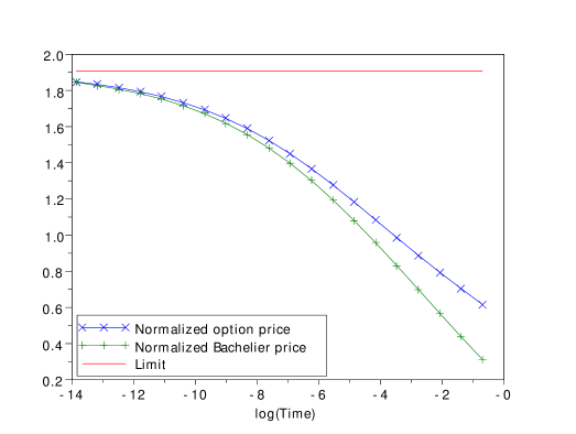
Figure 2. Convergence of the re-normalised price for ATM options: the parameter values of the tempered stable process, which models the log-stock are given in (37).

4.3. Convergence of option prices with variable strike

In this section we investigate numerically the convergence of the out-of-the-money (OTM) option prices given in Theorem 1. The parameter values for the underlying process are given in (37). Note that in the case of the tempered stable Lévy process with Lévy density (35), the limits in (4) of Theorem 1 take the form

$$\lim_{x\downarrow 0}x^{\alpha}\nu((x,\infty))=\lim_{x\downarrow 0}x^{\alpha}\nu((-\infty,-x))=\frac{c}{\alpha}.$$

Figure 3 shows the dependence of the normalised option and “Bachelier” prices, respectively given by

$$\frac{\mathbb{E}[(e^{X_{t}}-e^{k_{t}})^{+}]}{tk_{t}^{1-\alpha}}\qquad\text{ and }\qquad\frac{\mathbb{E}[(X_{t}-k_{t})^{+}]}{tk_{t}^{1-\alpha}},$$

on time to maturity in log-scale, where

$$k_{t}=t^{1/\alpha^{\prime}}\qquad\text{with}\qquad\alpha^{\prime}=1.9.$$

The horizontal dotted line shows the limiting value $\frac{c}{\alpha(\alpha-1)}=\frac{4}{3}$ predicted by Theorem 1.

Similarly, Figure 4 plots the dependence on time to maturity (on the log-scale) of the normalised option price

$$\frac{\mathbb{E}[(e^{X_{t}}-e^{k_{t}})^{+}]}{tk_{t}^{1-\alpha}}\qquad\text{for}\quad k_{t}=\theta\sqrt{t\log\frac{1}{t}}\qquad\text{and}\qquad\theta\in\{0.1,0.2,0.3\}.$$

As in Figure 3, the limiting horizontal dotted line is given be $\frac{c}{\alpha(\alpha-1)}=\frac{4}{3}$.

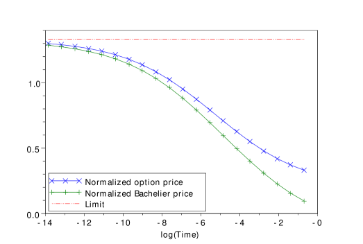
Figure 3. Convergence of the re-normalised price for OTM options: $k_{t}=t^{\frac{1}{\alpha^{\prime}}}$ with $\alpha^{\prime}=1.9$ and the other parameters of the process $X$ are given in (37).

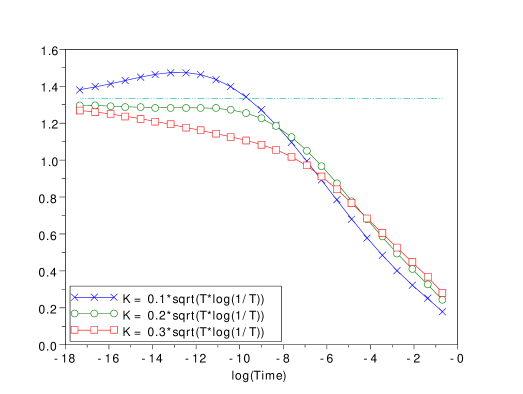
Figure 4. Convergence of the re-normalised price for OTM options: $k_{t}=\theta\sqrt{t\log\frac{1}{t}}$ with $\theta\in\{0.1,0.2,0.3\}$ and other parameters given in (37).

4.4. Convergence of the implied volatilities to the limiting smile

In this section we illustrate the convergence of the implied volatility (expressed as function of the re-normalised strike $\theta$) to the limit $\sigma_{0}(\theta)$ given in Corollary 4. In order to test the formula both with and without the diffusion component we fix two models: the first is a pure jump tempered stable Lévy process with the following parameter values

$$c_{+}=c_{-}=c=0.01,\qquad\lambda_{+}=\lambda_{-}=3,\qquad\alpha_{+}=\alpha_{-}=\alpha=1.5,$$

which correspond to the unit annualised volatility of about $14\%$. The second model is the same tempered stable process with an added diffusion component of volatility $\sigma=0.2$.

Recall that the limiting formula for positive $\theta$ is $\sigma_{0}(\theta)=\max\{\sigma,\frac{\theta}{\sqrt{2-\alpha}}\}$. Figure 5 plots the right wing of the implied volatility smile (as function of $\theta$) for different times to maturity when a diffusion component is present (left graph) and diffusion component is absent (right graph), together with the limiting shape $\sigma_{0}(\theta)$. The convergence to the limit is visible in both graphs but slow, because the error terms in Corollary 4 are logarithmic in time. Nevertheless, the following observations can be made already at “not such small” times:

• The smile is remarkably stable in time, when it is expressed as function of the re-normalised variable $\theta$. In particular, the slope of the wings predicted by Corollary 4 is achieved rather quickly.

• The distinction between the U-shaped smile in the presence of a diffusion component and the V-shaped smile in the pure jump case, is clearly visible.

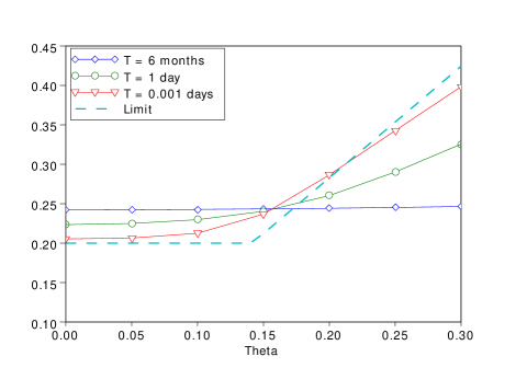
Figure 5. Convergence of the implied volatilities. Left: a diffusion component is present. Right: no diffusion component.

4.5. Approximation of the implied volatility for small times to maturity

In this section we illustrate the approximation of the implied volatility at small times by the asymptotic formula (24). We take the same parameters of the tempered stable process as in Section 4.4 and consider the case $\sigma=0$ (when the diffusion component is present, in the region where the pure jump component dominates, the asymptotic formula is the same, and in the diffusion-dominated region, there are no additional terms added to the constant limit). Figure 6 illustrates the quality of the approximation for $t=1$ day and $t=0.1$ days.

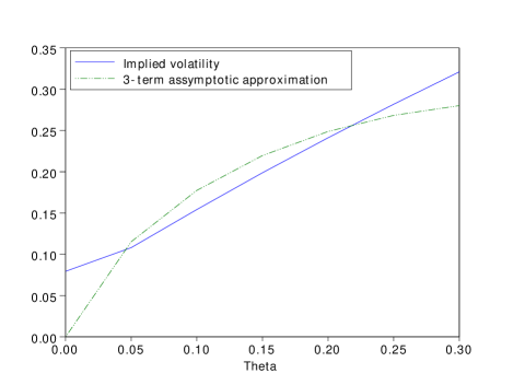
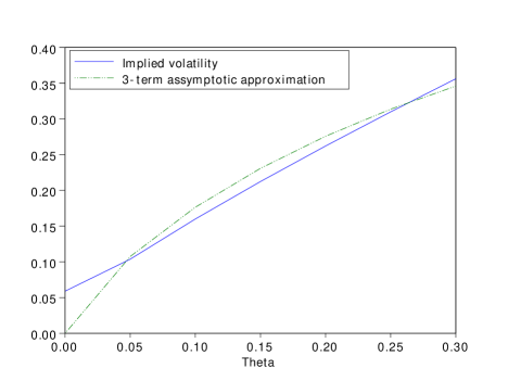
Figure 6. Approximation of the implied volatilities by the asymptotic formula (24). Left: $t=1$ day. Right: $t=0.1$ days.

5. Proofs

5.1. Proof of Theorem 1

By Lemma 5, to prove Theorem 1, it is sufficient to show that

(38) $$\mathbb{E}[(X_{t}-k_{t})^{+}]=\mathbb{E}[(\sigma W_{t}-k_{t})^{+}]+\frac{tk_{t}^{1-\alpha_{+}}c_{+}}{\alpha_{+}-1}+o(tk_{t}^{1-\alpha_{+}}+\mathbb{E}[(\sigma W_{t}-k_{t})^{+}])$$

as $t\downarrow 0$ for the call case and

(39) $$\mathbb{E}[(-k_{t}-X_{t})^{+}]=\mathbb{E}[(-k_{t}-\sigma W_{t})^{+}]+\frac{tk_{t}^{1-\alpha_{-}}c_{-}}{\alpha_{-}-1}+o(tk_{t}^{1-\alpha_{-}}+\mathbb{E}[(-k_{t}-\sigma W_{t})^{+}])$$

as $t\downarrow 0$ for the put case. Note that (39) follows from (38) by a substitution $X\mapsto-X$. Therefore, from now on we concentrate on the proof of (38), assuming with no loss of generality that $c_{+}>0$.

Step 1. In this first step, we assume that $\nu((-\infty,0))=0$ and would like to prove

(40) $$\mathbb{E}[(X_{t}-k_{t})^{+}]=\mathbb{E}[(\sigma W_{t}-k_{t})^{+}]+\frac{tk_{t}^{1-\alpha_{+}}c_{+}}{\alpha_{+}-1}+o(tk_{t}^{1-\alpha_{+}}).$$

Fix $t>0$, and $\varepsilon>0$ with $\varepsilon<\frac{1}{32}$, let $X^{t}$ be a Lévy process with no diffusion part, Lévy measure $\nu(dx)1_{\{0<x\leq\varepsilon k_{t}\}}$ and third component of the characteristic triplet

$$\gamma_{t}=\gamma-\int_{(\varepsilon k_{t},1]}z\nu(dz)$$

Let $(\xi^{t}_{i})_{i\geq 1}$ be a sequence of i.i.d. random variables with probability distribution

$$\frac{\nu(dz)1_{\{z>\varepsilon k_{t}\}}}{\nu(\{z:z>\varepsilon k_{t}\})},$$

and $N^{t}$ a standard Poisson process with intensity $\lambda_{t}:=\nu(\{z:z>\varepsilon k_{t}\})$. Furthermore we assume that $X^{t}$, $N^{t}$ and $(\xi^{t}_{i})_{i\geq 1}$ are independent. Then the following equality in law holds

(41) $$X_{t}\stackrel{{\scriptstyle d}}{{=}}\sigma W_{t}+X^{t}_{t}+\sum_{i=1}^{N^{t}_{t}}\xi^{t}_{i},$$

and it follows that

(42) $$\mathbb{E}\left[\left(X_{t}-k_{t}\right)^{+}\right] =e^{-\lambda_{t}t}\mathbb{E}\left[\left(\sigma W_{t}+X^{t}_{t}-k_{t}\right)^{+}\right]$$

(43) $$+\lambda_{t}te^{-\lambda_{t}t}\mathbb{E}\left[\left(\sigma W_{t}+X^{t}_{t}+\xi^{t}_{1}-k_{t}\right)^{+}\right]$$

(44) $$+e^{-\lambda_{t}t}\sum_{k\geq 2}\frac{(\lambda_{t}t)^{k}}{k!}\mathbb{E}\left[\left(\sigma W_{t}+X^{t}_{t}+\sum_{i=1}^{k}\xi^{t}_{i}-k_{t}\right)^{+}\right].$$

As a preliminary computation, we deduce from the assumptions of the theorem that the following asymptotic behaviour holds as $t\downarrow 0$ (recall definition (3a)):

(45) $$\lambda_{t}\sim c_{+}(\varepsilon k_{t})^{-\alpha_{+}},\quad\Sigma_{t}:=\int_{(0,k_{t}\varepsilon]}z^{2}\nu(dz)\sim\frac{2c_{+}}{2-\alpha_{+}}(\varepsilon k_{t})^{2-\alpha_{+}},$$

(46) $$\gamma_{t}\sim\frac{c_{+}}{(\varepsilon k_{t})^{\alpha_{+}-1}},\quad\mathbb{E}[(X_{t}^{t})^{2}]=t^{2}(\gamma_{t})^{2}+t\Sigma_{t}\sim t\Sigma_{t},\quad\mathbb{E}[\xi^{t}_{1}]\sim\frac{\alpha_{+}}{\alpha_{+}-1}\varepsilon k_{t},$$

$$\mathbb{E}[(X_{t}^{t})^{4}]=t\int_{(0,k_{t}\varepsilon]}z^{4}\nu(dz)+4t^{2}\gamma_{t}\int_{(0,k_{t}\varepsilon]}z^{3}\nu(dz)+3t^{2}\Sigma_{t}^{2}+6t^{3}\gamma_{t}^{2}\Sigma_{t}+t^{4}\gamma_{t}^{4}$$

(47) $$\qquad\qquad\sim\frac{4c_{+}}{4-\alpha_{+}}tk_{t}^{4-\alpha_{+}}.$$

To estimate the term in (42), we apply the argument inspired by Lemma 2 in [19]. In the current notation this implies

(48) $$\mathbb{P}[X^{t}_{t}>k_{t}]\leq\exp\left\{-t\int_{\gamma_{t}}^{k_{t}/t}\tau(z)dz\right\},$$

where $\tau:[\gamma_{t},\infty)\to\mathbb{R}$ is the inverse function of $s:[0,\infty)\to\mathbb{R}$ defined by

$$s(x)=\gamma_{t}+\int_{(0,k_{t}\varepsilon]}z(e^{zx}-1)\nu(dz).$$

By Taylor’s theorem, this function satisfies

$$s(x)\leq\gamma_{t}+xe^{k_{t}\varepsilon x}\Sigma_{t}\leq\gamma_{t}+\frac{e^{2k_{t}\varepsilon x}-1}{k_{t}\varepsilon}\Sigma_{t}.$$

This implies that

$$\tau(z)\geq\frac{1}{2k_{t}\varepsilon}\log\left\{1+\frac{z-\gamma_{t}}{\Sigma_{t}}k_{t}\varepsilon\right\},$$

and therefore, substituting this into (48),

$$\mathbb{P}[X^{t}_{t}>k_{t}] \leq\exp\left\{-\frac{t\Sigma_{t}}{2(k_{t}\varepsilon)^{2}}\int_{0}^{\frac{k_{t}\varepsilon}{\Sigma_{t}}(k_{t}/t-\gamma_{t})}\log(1+s)ds\right\}$$

(49) $$\leq\exp\left\{-\frac{k_{t}-\gamma_{t}t}{2k_{t}\varepsilon}\log\left(\frac{k_{t}\varepsilon}{e\Sigma_{t}}(k_{t}/t-\gamma_{t})\right)\right\}$$

From the assumptions of the theorem and (45)–(47), there exists $t_{1}>0$ such that $t<t_{0}$ implies

$$\mathbb{P}[X^{t}_{t}>k_{t}]\leq\exp\left\{-\frac{1}{4\varepsilon}\log\left(\frac{k_{t}^{2}\varepsilon}{2et\Sigma_{t}}\right)\right\}=\left(\frac{k_{t}^{2}\varepsilon}{2et\Sigma_{t}}\right)^{-\frac{1}{4\varepsilon}}\leq C(tk_{t}^{-\alpha_{+}})^{\frac{1}{4\varepsilon}}\leq C(tk_{t}^{-\alpha_{+}})^{8}$$

for some constant $C<\infty$. By similar arguments it can be shown that

(50) $$\mathbb{P}\left[X^{t}_{t}>\frac{k_{t}}{2}\right]\leq C(tk_{t}^{-\alpha_{+}})^{4}.$$

Coming back to the estimation of (42), we first deal with the case $\sigma=0$. In this case, the Cauchy-Schwartz inequality allows to conclude that

$$\mathbb{E}\left[\left(X^{t}_{t}-k_{t}\right)^{+}\right]\leq\mathbb{E}\left[\left({X^{t}_{t}}\right)^{2}\right]^{\frac{1}{2}}\mathbb{P}[X^{t}_{t}>k_{t}]^{\frac{1}{2}}=O(k_{t}(tk_{t}^{-\alpha_{+}})^{2}),$$

because the first factor remains bounded by (45)–(47).

Let us now focus on the case $\sigma>0$. Let $f(x):=\frac{1}{\sqrt{2\pi}}\int_{x}^{\infty}(z-x)e^{-\frac{z^{2}}{2}}dz$. The expectation in (42) can be expressed as

$$\mathbb{E}[(\sigma W_{t}+X^{t}_{t}-k_{t})^{+}]=\sigma\sqrt{t}\mathbb{E}\left[f\left(\frac{k_{t}-X^{t}_{t}}{\sigma\sqrt{t}}\right)\right].$$

By Taylor’s formula, we then get

$$\mathbb{E}[(\sigma W_{t}+X^{t}_{t}-k_{t})^{+}]=\sigma\sqrt{t}f\left(\frac{k_{t}}{\sigma\sqrt{t}}\right)-f^{\prime}\left(\frac{k_{t}}{\sigma\sqrt{t}}\right)\mathbb{E}[X^{t}_{t}]$$

$$\qquad\qquad+\frac{1}{\sigma\sqrt{t}}\mathbb{E}\left[(X_{t}^{t})^{2}\int_{0}^{1}(1-\theta)f^{\prime\prime}\left(\frac{k_{t}-\theta X^{t}_{t}}{\sigma\sqrt{t}}\right)d\theta\right]$$

$$=\mathbb{E}[(\sigma W_{t}-k_{t})^{+}]+\gamma_{t}t\mathbb{P}[\sigma W_{t}>k_{t}]+\frac{1}{\sigma\sqrt{2\pi t}}\mathbb{E}\left[(X_{t}^{t})^{2}\int_{0}^{1}(1-\theta)e^{-\frac{1}{2}\left(\frac{k_{t}-\theta X^{t}_{t}}{\sigma\sqrt{t}}\right)^{2}}d\theta\right].$$

We now need to show that the second and the third terms do not contribute to the limit. Since by assumption $\frac{\sqrt{t}}{k_{t}}\to 0$, we have that $\mathbb{P}[\sigma W_{t}>k_{t}]\to 0$ as $t\to 0$, and therefore, by (45)–(47),

$$\gamma_{t}t\mathbb{P}[\sigma W_{t}>k_{t}]=o(tk_{t}^{1-\alpha_{+}}).$$

The last term can be split into two terms, which are easy to estimate using (45)–(47):

$$\frac{1}{\sqrt{t}}\mathbb{E}\left[(X_{t}^{t})^{2}1_{\{X^{t}_{t}\leq\frac{k_{t}}{2}\}}\int_{0}^{1}(1-\theta)e^{-\frac{1}{2}\left(\frac{k_{t}-\theta X^{t}_{t}}{\sigma\sqrt{t}}\right)^{2}}d\theta\right]\leq\frac{1}{\sqrt{t}}\mathbb{E}[(X_{t}^{t})^{2}]e^{-\frac{1}{8}\left(\frac{k_{t}}{\sigma\sqrt{t}}\right)^{2}}$$

$$=O(tk_{t}^{1-\alpha_{+}})\frac{k_{t}}{\sqrt{t}}e^{-\frac{1}{8}\left(\frac{k_{t}}{\sigma\sqrt{t}}\right)^{2}}=o(tk_{t}^{1-\alpha_{+}}),$$

because by assumption of the theorem, $\frac{k_{t}}{\sqrt{t}}\to\infty$. On the other hand,

$$\frac{1}{\sqrt{t}}\mathbb{E}\left[(X_{t}^{t})^{2}1_{\{X^{t}_{t}>\frac{k_{t}}{2}\}}\int_{0}^{1}(1-\theta)e^{-\frac{1}{2}\left(\frac{k_{t}-\theta X^{t}_{t}}{\sigma\sqrt{t}}\right)^{2}}d\theta\right]\leq\frac{1}{\sqrt{t}}\mathbb{E}\left[(X_{t}^{t})^{2}1_{\{X^{t}_{t}>\frac{k_{t}}{2}\}}\right]$$

$$\leq\frac{1}{\sqrt{t}}\mathbb{E}[(X_{t}^{t})^{4}]^{\frac{1}{2}}\mathbb{P}[X^{t}_{t}>\frac{k_{t}}{2}]^{\frac{1}{2}}=O(k_{t}^{2-\frac{\alpha_{+}}{2}})O((tk_{t}^{-\alpha_{+}})^{2})=o(tk_{t}^{1-\alpha_{+}})$$

by (47) and (50). We have therefore shown that

$$\mathbb{E}[(\sigma W_{t}+X^{t}_{t}-k_{t})^{+}]=\mathbb{E}[(\sigma W_{t}-k_{t})^{+}]+o(tk_{t}^{1-\alpha_{+}}).$$

From (45), the assumption on $k_{t}$ in Theorem 1 and the Lipschitz property of the function $x\mapsto x^{+}$, it follows that

$$e^{-\lambda_{t}t}\mathbb{E}[(\sigma W_{t}+X^{t}_{t}-k_{t})^{+}]=\mathbb{E}[(\sigma W_{t}-k_{t})^{+}]+o(tk_{t}^{1-\alpha_{+}})$$

as well.

For the term in (43), the Lipschitz property of the function $x\mapsto x^{+}$, (45)–(47) and the assumption of the theorem (i.e. the first assumption on $k_{t}$ in Theorem 1 in the case $\sigma=0$ and the second one otherwise) imply the following estimate:

$$\lambda_{t}t\left|\mathbb{E}\left[\left(\sigma W_{t}+X^{t}_{t}+\xi^{t}_{1}-k_{t}\right)^{+}\right]-\mathbb{E}\left[\left(\xi^{t}_{1}-k_{t}\right)^{+}\right]\right|\leq\lambda_{t}t\{{\mathbb{E}[|X_{t}^{t}|]}+\sigma\mathbb{E}[|W_{t}|]\}$$

$$\leq\lambda_{t}t\{\mathbb{E}[|X_{t}^{t}|^{2}]^{1/2}+\sigma\sqrt{t}\}=O(\lambda_{t}t^{\frac{3}{2}}\Sigma_{t}^{\frac{1}{2}})+\sigma\lambda_{t}t^{\frac{3}{2}}=o(tk_{t}^{1-\alpha_{+}})\quad\text{as $t\to 0$}.$$

On the other hand, integration by parts implies

$$\lambda_{t}t\mathbb{E}\left[\left(\xi^{t}_{1}-k_{t}\right)^{+}\right]=t\int_{k_{t}}^{\infty}\left(z-k_{t}\right)\nu(dz)=t\int_{k_{t}}^{\infty}U(z)dz\sim\frac{tk_{t}^{1-\alpha_{+}}c_{+}}{\alpha_{+}-1}\quad\text{as $t\to 0$},$$

where $U(z):=\nu((z,\infty))$, which yields the second term in (5).

To treat the summand in (44), observe that by (45)–(47), for $k\geq 2$,

$$\mathbb{E}\left[\left(\sigma W_{t}+X^{t}_{t}+\sum_{i=1}^{k}\xi^{t}_{i}-k_{t}\right)^{+}\right]\leq\sigma\sqrt{t}+\mathbb{E}[|X^{t}_{t}|^{2}]^{1/2}+k\mathbb{E}[\xi^{t}_{1}]$$

$$=\sigma\sqrt{t}+O(t^{1/2}k_{t}^{1-\alpha_{+}/2})+kO(k_{t})=kO(k_{t}).$$

Therefore, the summand in (44) is of order $O(k_{t}\lambda^{2}_{t}t^{2})=O(k_{t}(tk_{t}^{-\alpha_{+}})^{2})$ and hence $o(tk_{t}^{1-\alpha_{+}})$.

Step 2. We now treat the case when $\nu((-\infty,0))\neq 0$. Let $X^{-}$ be a spectrally negative Lévy process with zero mean and zero diffusion part and $Y$ be a spectrally positive Lévy process such that $X^{-}+Y\stackrel{{\scriptstyle d}}{{=}}X$. Let $\beta\in(\max(\alpha_{+},\alpha_{-}),\alpha)$ (where we take $\alpha=2$ is $\sigma>0$) and $\chi_{t}=t^{\frac{1}{\beta}}$. As before, we fix $\varepsilon>0$ and let $\bar{X}^{t}$ be a Lévy process with no diffusion part, zero mean and Lévy measure $\nu(dx)1_{\{-\varepsilon\chi_{t}\leq x<0\}}$, let $\bar{\gamma}_{t}=\int_{(-\infty,-\varepsilon\chi_{t})}z\nu(dz)$, let $(\bar{\xi}^{t}_{i})_{i\geq 1}$ be a sequence of i.i.d. random variables with probability distribution

$$\frac{\nu(dz)1_{\{z<\varepsilon\chi_{t}\}}}{\nu(\{z:z<\varepsilon\chi_{t}\})}$$

and finally $\bar{\lambda}_{t}=\nu(\{z:z<\varepsilon\chi_{t}\})$. With a decomposition similar to (42)–(44), it is easy to show that the option price $\mathbb{E}[(X_{t}-k_{t})^{+}]$ admits an upper bound

$$\mathbb{E}[(X_{t}-k_{t})^{+}] =\mathbb{E}[(X^{-}_{t}+Y_{t}-k_{t})^{+}]\leq\mathbb{E}[(\bar{X}^{t}_{t}+\bar{\gamma}_{t}t+Y_{t}-k_{t})^{+}]$$

$$\leq\mathbb{E}[(Y_{t}+\chi_{t}-k_{t})^{+}]\mathbb{P}[\bar{X}^{t}_{t}\leq\chi_{t}]+\mathbb{E}[X_{t}^{2}]^{\frac{1}{2}}\mathbb{P}[\bar{X}^{t}_{t}>\chi_{t}]^{\frac{1}{2}}$$

and a lower bound

$$\mathbb{E}[(X_{t}-k_{t})^{+}] =\mathbb{E}[(X^{-}_{t}+Y_{t}-k_{t})^{+}]\geq e^{-\bar{\lambda}_{t}t}\mathbb{E}[(\bar{X}^{t}_{t}+\bar{\gamma}_{t}t+Y_{t}-k_{t})^{+}]$$

$$\geq e^{-\bar{\lambda}_{t}t}\mathbb{P}[\bar{X}^{t}_{t}\geq-\chi_{t}]\mathbb{E}[(-\chi_{t}+\bar{\gamma}_{t}t+Y_{t}-k_{t})^{+}]$$

Similarly to (45)–(47), we have

$$\bar{\Sigma}_{t}:=\int_{(-\varepsilon\chi_{t},0)}z^{2}\nu(dz)\sim\frac{2}{2-\alpha_{-}}(\varepsilon\chi_{t})^{2-\alpha_{-}},$$

and with the same logic as in (49), we have that

$$\mathbb{P}[\bar{X}^{t}_{t}>\chi_{t}]\leq\left(\frac{\chi_{t}^{2}\varepsilon}{e\bar{\Sigma}_{t}t}\right)^{\frac{1}{2\varepsilon}}\sim\left(t^{\frac{\alpha_{-}}{\beta}-1}\right)^{\frac{1}{2\varepsilon}},\quad t\to 0.$$

It is now clear that one can choose $\varepsilon>0$ so that the square root of this expression becomes equal to $o(tk_{t}^{1-\alpha_{+}})$. Since $\mathbb{P}[\bar{X}^{t}_{t}<-\chi_{t}]$ admits the same estimate, and $t\bar{\lambda}_{t}\to 0$ as $t\to 0$, we get that

$$\mathbb{E}[(X_{t}-k_{t})^{+}] \geq m_{t}\mathbb{E}[(Y_{t}-\chi_{t}+\bar{\gamma}_{t}t-k_{t})^{+}]$$

$$\mathbb{E}[(X_{t}-k_{t})^{+}] \leq M_{t}\mathbb{E}[(Y_{t}+\chi_{t}-k_{t})^{+}]+o(tk_{t}^{1-\alpha_{+}}),$$

where $m_{t}$ and $M_{t}$ converge to $1$ as $t\to 0$. Since $\chi_{t}=o(k_{t})$ and $\bar{\gamma}_{t}t=o(k_{t})$, from (40), we then get

$$\mathbb{E}[(X_{t}-k_{t})^{+}] \geq m_{t}\mathbb{E}[(\sigma W_{t}-\chi_{t}+\bar{\gamma}_{t}t-k_{t})^{+}]+m_{t}\frac{t(k_{t}+\chi_{t}-\bar{\gamma}_{t}t)^{1-\alpha_{+}}c_{+}}{\alpha_{+}-1}+o(tk_{t}^{1-\alpha_{+}})$$

$$=m_{t}\mathbb{E}[(\sigma W_{t}-\chi_{t}+\bar{\gamma}_{t}t-k_{t})^{+}]+\frac{tk_{t}^{1-\alpha_{+}}c_{+}}{\alpha_{+}-1}+o(tk_{t}^{1-\alpha_{+}})$$

$$\mathbb{E}[(X_{t}-k_{t})^{+}] \leq M_{t}\mathbb{E}[(\sigma W_{t}+\chi_{t}-k_{t})^{+}]+M_{t}\frac{t(k_{t}-\chi_{t})^{1-\alpha_{+}}c_{+}}{\alpha_{+}-1}+o(tk_{t}^{1-\alpha_{+}})$$

$$=M_{t}\mathbb{E}[(\sigma W_{t}+\chi_{t}-k_{t})^{+}]+\frac{tk_{t}^{1-\alpha_{+}}c_{+}}{\alpha_{+}-1}+o(tk_{t}^{1-\alpha_{+}})$$

Finally, since we also have $\chi_{t}=o(\sqrt{t})$ and $\bar{\gamma}_{t}t=o(\sqrt{t})$, we get that $\mathbb{E}[(\sigma W_{t}-\chi_{t}+\bar{\gamma}_{t}t-k_{t})^{+}]\sim\mathbb{E}[(\sigma W_{t}-k_{t})^{+}]$ and $\mathbb{E}[(\sigma W_{t}+\chi_{t}-k_{t})^{+}]\sim\mathbb{E}[(\sigma W_{t}-k_{t})^{+}]$, which allows to complete the proof of Theorem 1.

5.2. Proof of Proposition 2

We first concentrate on the proof of (9). Let $(\sigma^{2},\nu,b)$ be the characteristic triplet of $X$ with respect to zero truncation function, meaning that

$$X_{t}=bt+\sigma W_{t}+\sum_{s\leq t}\Delta X_{s},$$

where as usual for any $s>0$ we define $\Delta X_{s}=X_{s}-X_{s-}$.

Assume first that $\sigma=0$. The left-derivative of the function

$$x\mapsto(e^{-k_{t}}-e^{x})^{+}\qquad\text{is}\qquad x\mapsto-e^{x}1_{\{x\leq-k_{t}\}},$$

and hence Itô-Tanaka formula [16, Ch. IV, Thm. 70] applied to the process $(e^{-k_{t}}-e^{X})^{+}$ yields

$$(e^{-k_{t}}-e^{X_{t}})^{+} = -\int_{(0,t]}e^{X_{s-}}1_{\{X_{s-}\leq-k_{t}\}}dX_{s}$$

$$+ \sum_{0<s\leq t}\left[(e^{-k_{t}}-e^{X_{s}})^{+}-(e^{-k_{t}}-e^{X_{s-}})^{+}+e^{X_{s-}}1_{\{X_{s-}\leq-k_{t}\}}\Delta X_{s}\right]$$

$$= -b\int_{0}^{t}e^{X_{s-}}1_{\{X_{s-}\leq-k_{t}\}}ds+\sum_{0<s\leq t}\left[(e^{-k_{t}}-e^{X_{s-}+\Delta X_{s}})^{+}-(e^{-k_{t}}-e^{X_{s-}})^{+}\right]$$

for any $t\geq 0$, since, in this case, $X$ has paths of finite variation. Since $(\Delta X_{s})_{s\geq 0}$ is a Poisson point process with intensity measure $\nu(dy)\times ds$, and $X_{s-}\neq X_{s}$ for at most countably many time $s$ in the interval $[0,t]$ almost surely, taking expectations on both sides of the path-wise representation above and applying the compensation formula for point processes yields

$$\mathbb{E}[(e^{-k_{t}}-e^{X_{t}})^{+}] = -b\mathbb{E}\left[\int_{0}^{t}e^{X_{s}}1_{\{X_{s}\leq-k_{t}\}}ds\right]$$

$$+ \mathbb{E}\left[\int_{0}^{t}\int_{\mathbb{R}\setminus\{0\}}\left\{(e^{-k_{t}}-e^{X_{s}+y})^{+}-(e^{-k_{t}}-e^{X_{s}})^{+}\right\}\nu(dy)ds\right].$$

From Theorem 43.20 in [20], we have that $\frac{X_{t}}{t}\to b$ almost surely as $t\to 0$. Therefore, for any $\varepsilon>0$, each path $X(\omega)$ satisfies the following inequalities

$$X_{t}(\omega)>t(b-\varepsilon)>-k_{t}\qquad\text{for all small enough}\qquad t>0$$

(recall that by assumption $k_{t}/t\to\infty$ as $t\downarrow 0$). Furthermore, since $k_{t}\downarrow 0$ as $t\downarrow 0$, for all sufficiently small $t$ we have $X_{s}(\omega)>-k_{t}$ for all $s\leq t$. Therefore it holds $\frac{1}{t}\int_{0}^{t}e^{X_{s}}1_{\{X_{s}\leq-k_{t}\}}ds\to 0$ almost surely. Since on the other hand we have

$$\frac{1}{t}\int_{0}^{t}e^{X_{s}}1_{\{X_{s}\leq-k_{t}\}}ds\leq\frac{1}{t}\int_{0}^{t}e^{-k_{t}}ds=e^{-k_{t}},$$

the dominated convergence theorem implies

$$\mathbb{E}\left[\int_{0}^{t}e^{X_{s}}1_{\{X_{s}\leq-k_{t}\}}ds\right]=o(t)\quad\text{as $t\to 0$}.$$

To deal with the second term in (5.2), observe that for any $\varepsilon>0$, each path $X(\omega)$ satisfies the inequalities $(b-\varepsilon)t\leq X_{t}(\omega)\leq(b+\varepsilon)t$ for all $t$ sufficiently small. Therefore $X(\omega)$ also satisfies the following inequalities for any $y\in\mathbb{R}\setminus\{0\}$ and all sufficiently small times $t>0$:

$$(e^{-k_{t}}-e^{X_{s}(\omega)+y})^{+}-(e^{-k_{t}}-e^{X_{s}(\omega)})^{+}\leq(e^{-k_{t}}-e^{(b-\varepsilon)t+y})^{+}-(e^{-k_{t}}-e^{(b-\varepsilon)t})^{+}$$

and

$$(e^{-k_{t}}-e^{X_{s}(\omega)+y})^{+}-(e^{-k_{t}}-e^{X_{s}(\omega)})^{+}\geq(e^{-k_{t}}-e^{(b+\varepsilon)t+y})^{+}-(e^{-k_{t}}-e^{(b+\varepsilon)t})^{+}.$$

The second term in both sides of the above inequalities is in fact always zero for sufficiently small $t$. Therefore we get the following almost sure convergence:

$$\frac{1}{t}\int_{0}^{t}\int_{\mathbb{R}\setminus\{0\}}\left\{(e^{-k_{t}}-e^{X_{s}+y})^{+}-(e^{-k_{t}}-e^{X_{s}})^{+}\right\}\nu(dy)ds\to\int_{\mathbb{R}\setminus\{0\}}(1-e^{y})^{+}\nu(dy)\qquad\text{as $t\downarrow 0$.}$$

Since the function $y\mapsto(e^{-k_{t}}-e^{X_{s}+y})^{+}$ is Lipschitz with a Lipschitz constant that does not depend on the path $X(\omega)$, the dominated convergence theorem and the representation in (5.2) yield

$$\lim_{t\downarrow 0}\frac{1}{t}\mathbb{E}[(e^{-k_{t}}-e^{X_{t}})^{+}]=\int_{\mathbb{R}\setminus\{0\}}(1-e^{y})^{+}\nu(dy).$$

Assume now that $\sigma>0$. Define

$$f(t,x):=\mathbb{E}\left[\left(1-e^{x+k_{t}+\sigma W_{t}-\frac{\sigma^{2}}{2}t}\right)^{+}\right]\qquad\text{and}\qquad Z_{t}:=\left(b+\frac{\sigma^{2}}{2}\right)t+\sum_{0<s\leq t}\Delta X_{s}$$

and note that

(52) $$\mathbb{E}[(e^{-k_{t}}-e^{X_{t}})^{+}]=e^{-k_{t}}\mathbb{E}[f(t,Z_{t})].$$

The derivative of $f$ with respect to $x$ is given by

(53) $$f^{\prime}(t,x):=-\mathbb{E}\left[e^{x+k_{t}+\sigma W_{t}-\frac{\sigma^{2}}{2}t}1_{\{x+k_{t}+\sigma W_{t}-\frac{\sigma^{2}}{2}t\leq 0\}}\right]\geq-1,$$

It can be computed explicitly as

(54) $$f^{\prime}(t,x)=-e^{x+k_{t}}N\left(-\frac{\frac{1}{2}\sigma^{2}t+x+k_{t}}{\sigma\sqrt{t}}\right),$$

where $N(\cdot)$ denotes the standard normal CDF. Note also for future use that

(55) $$f^{\prime\prime}(t,x)=-e^{x+k_{t}}N\left(-\frac{\frac{1}{2}\sigma^{2}t+x+k_{t}}{\sigma\sqrt{t}}\right)+\frac{1}{\sigma\sqrt{t}}n\left(\frac{-\frac{1}{2}\sigma^{2}t+x+k_{t}}{\sigma\sqrt{t}}\right)\geq-1,$$

with $n(x)=N^{\prime}(x)$.

Applying Itô’s formula to the process $f(t,Z)$ as a function of $Z$ with $t$ fixed, yields

$$f(t,Z_{t}) = f(t,0)+\int_{(0,t]}f^{\prime}(t,Z_{s-})dZ_{s}+\sum_{0<s\leq t}\left[f(t,Z_{s})-f(t,Z_{s-})-f^{\prime}(t,Z_{s-})\Delta Z_{s}\right]$$

$$= f(t,0)+\left(b+\frac{\sigma^{2}}{2}\right)\int_{0}^{t}f^{\prime}(t,Z_{s-})ds+\sum_{0<s\leq t}\left[f(t,Z_{s-}+\Delta X_{s})-f(t,Z_{s-})\right],$$

since $\Delta Z_{s}=\Delta X_{s}$ for all $s>0$. By taking the expectation and applying (52) we find

(56) $$\mathbb{E}[(e^{-k_{t}}-e^{X_{t}})^{+}] =e^{-k_{t}}\mathbb{E}[f(t,0)]+e^{-k_{t}}\mathbb{E}\left[\int_{0}^{t}f^{\prime}(t,Z_{s})ds\right]$$

$$\qquad\qquad+e^{-k_{t}}\mathbb{E}\left[\int_{0}^{t}\int_{\mathbb{R}\setminus\{0\}}\left\{f(t,Z_{s}+y)-f(t,Z_{s})\right\}\nu(dy)ds\right].$$

The first term on the right-hand side of (56) is equal to the first term on the right-hand side of (9). As in the case $\sigma=0$, using the almost sure convergence $\frac{Z_{t}}{t}\to b+\frac{\sigma^{2}}{2}$, the explicit form (54) of $f^{\prime}(t,x)$ and the assumption that $\frac{k_{t}}{\sqrt{t}}\to\infty$ as $t\downarrow 0$, we get that

$$\frac{1}{t}\int_{0}^{t}f^{\prime}(t,Z_{s})ds\to 0$$

almost surely. Since $|f^{\prime}(t,Z_{s})|\leq 1$ for all $t,s\geq 0$ by (53), the dominated convergence theorem yields

$$\mathbb{E}\left[\int_{0}^{t}f^{\prime}(t,Z_{s})ds\right]=o(t).$$

To treat the last term in (56), we use the fact that for any $\varepsilon>0$, each path $Z(\omega)$ satisfies the inequalities

$$t(b+\sigma^{2}/2-\varepsilon)\leq Z_{t}(\omega)\leq t(b+\sigma^{2}/2+\varepsilon).$$

for all sufficiently small $t$. Therefore, since $f^{{}^{\prime\prime}}(t,x)\geq-1$, the following inequalities hold

(57) $$f^{\prime}(t,t(b-\varepsilon+\sigma^{2}/2)+\theta y)-2t\varepsilon\leq f^{\prime}(t,Z_{s}(\omega)+\theta y)\leq f^{\prime}(t,t(b+\varepsilon+\sigma^{2}/2)+\theta y)+2t\varepsilon$$

for any trajectory $s\mapsto Z_{s}(\omega)$, where $s\in[0,t]$, and all sufficiently small $t$. The random variable under the expectation in the last term on the right-hand side of (56) can be expressed as follows:

(58) $$\frac{1}{t}\int_{0}^{t}\int_{\mathbb{R}\setminus\{0\}}\left\{f(t,Z_{s}+y)-f(t,Z_{s})\right\}\nu(dy)ds=\frac{1}{t}\int_{0}^{t}ds\int_{0}^{1}d\theta\int_{\mathbb{R}\setminus\{0\}}yf^{\prime}(t,Z_{s}+\theta y)\nu(dy).$$

The path-wise bounds in (57) can be used to estimate (58) from above and below. For each path $Z(\omega)$ we have the following bound for $y\in(-\infty,0)$ and all sufficiently small $t$:

$$2t\varepsilon\int_{(-\infty,0)}y\nu(dy)+\int_{0}^{1}d\theta\int_{(-\infty,0)}yf^{\prime}(t,t(b+\varepsilon+\sigma^{2}/2)+\theta y)\nu(dy)$$

$$\leq\frac{1}{t}\int_{0}^{t}ds\int_{0}^{1}d\theta\int_{(-\infty,0)}yf^{\prime}(t,Z_{s}(\omega)+\theta y)\nu(dy)$$

$$\leq-2t\varepsilon\int_{(-\infty,0)}y\nu(dy)+\int_{0}^{1}d\theta\int_{(-\infty,0)}yf^{\prime}(t,t(b-\varepsilon+\sigma^{2}/2)+\theta y)\nu(dy).$$

The explicit form (54) of $f^{\prime}(t,x)$ implies that for all $y<0$ and $\theta>0$ we have

$$f^{\prime}(t,t(b\pm\varepsilon+\sigma^{2}/2)+\theta y)\to-e^{\theta y}\qquad\text{as $t\to 0$.}$$

Since $f^{\prime}(t,x)$ is bounded, the dominated convergence theorem yields

$$\int_{0}^{1}d\theta\int_{(-\infty,0)}yf^{\prime}(t,t(b\pm\varepsilon+\sigma^{2}/2)+\theta y)\nu(dy)\to-\int_{0}^{1}d\theta\int_{(-\infty,0)}ye^{\theta y}\nu(dy)=\int_{(-\infty,0)}\nu(dy)(1-e^{y})$$

as $t\downarrow 0$. Formula (54) for $f^{\prime}(t,x)$ implies that for all $y\in(0,\infty)$ and $\theta>0$ we have

$$f^{\prime}(t,t(b\pm\varepsilon+\sigma^{2}/2)+\theta y)\to 0\qquad\text{as $t\to 0$.}$$

An analogous argument for $y\in(0,\infty)$ to the one above and the representation in (58) imply the almost sure convergence

$$\frac{1}{t}\int_{0}^{t}\int_{\mathbb{R}\setminus\{0\}}\left\{f(t,Z_{s}+y)-f(t,Z_{s})\right\}\nu(dy)ds\to\int_{\mathbb{R}\setminus\{0\}}(1-e^{y})^{+}\nu(dy)\qquad\text{as $t\to 0$.}$$

Finally, since $f(t,x)$ is Lipschitz in $x$, with the Lipschitz constant independent of $t$, the dominated convergence theorem implies

$$\frac{1}{t}\mathbb{E}\left[\int_{0}^{t}\int_{\mathbb{R}\setminus\{0\}}\left\{f(t,Z_{s}+y)-f(t,Z_{s})\right\}\nu(dy)ds\right]\to\int_{\mathbb{R}\setminus\{0\}}(1-e^{y})^{+}\nu(dy).$$

This concludes the proof of (9). Note that in this proof, we did not use the condition in (2), but only the assumption $\int_{\mathbb{R}\setminus\{0\}}|x|\nu(dx)<\infty$.

We now concentrate on the proof of (8). Since the Lévy process $X$ satisfies (2), we can define the share measure $\widetilde{\mathbb{P}}$, via $\frac{d\widetilde{\mathbb{P}}}{d\mathbb{P}}|_{\mathcal{F}_{t}}=e^{X_{t}}$, as in the proof of Theorem 3. Analogous to the equality in (34), we have

(59) $$\mathbb{E}[(e^{X_{t}}-e^{k_{t}})^{+}]=e^{k_{t}}\widetilde{\mathbb{E}}[(e^{-k_{t}}-e^{-X_{t}})^{+}],$$

where $\widetilde{\mathbb{E}}$ denotes the expectation under the share measure $\widetilde{\mathbb{P}}$. Furthermore, it is well-known that under the measure $\widetilde{\mathbb{P}}$, the process $X$ is again a Lévy process with a characteristic triplet $(\sigma^{2},\widetilde{\nu},\widetilde{\gamma})$, where $\widetilde{\nu}(dx)=e^{x}\nu(dx)$, and $e^{-X}$ is a positive $\widetilde{\mathbb{P}}$-martingale started at one. The Lévy measure $\widetilde{\nu}$ clearly satisfies

$$\int_{\mathbb{R}\setminus\{0\}}|x|\widetilde{\nu}(dx)<\infty.$$

Therefore we can apply (9) to the process $-X$ under the measure $\widetilde{\mathbb{P}}$. Hence the identity in (59) yields:

$$\mathbb{E}[(e^{X_{t}}-e^{k_{t}})^{+}] =e^{k_{t}}\mathbb{E}[(e^{-k_{t}}-e^{\sigma W_{t}-\frac{\sigma^{2}t}{2}})^{+}]+te^{k_{t}}\int_{(0,\infty)}(1-e^{-x})\widetilde{\nu}(dx)+o(t)$$

$$=\mathbb{E}[(e^{\sigma W_{t}-\frac{\sigma^{2}t}{2}}-e^{k_{t}})^{+}]+t\int_{(0,\infty)}(e^{x}-1)\nu(dx)+o(t),$$

where we used the Black-Scholes put-call symmetry given in (32), the fact $e^{k_{t}}=1+o(1)$ and the equality $\widetilde{\nu}(dx)=e^{x}\nu(dx)$. This establishes the formula in (8) and concludes the proof of Proposition 2.

Appendix

Lemma 5.

Let $X$ be a Lévy process satisfying (2) and $k_{t}$ a deterministic function such that

$$k_{t}>0\quad\forall t>0\quad\text{and}\quad\lim_{t\downarrow}k_{t}=0\quad\text{as $t\downarrow 0$}.$$

Then for any $b\in\mathbb{R}$ we have

$$\mathbb{E}[(e^{X_{t}+bt}-e^{k_{t}})^{+}] =e^{k_{t}}\mathbb{E}[(X_{t}-k_{t})^{+}]+O(t)\quad\text{as $t\downarrow 0$,}$$

$$\mathbb{E}[(e^{-k_{t}}-e^{X_{t}+bt})^{+}] =e^{-k_{t}}\mathbb{E}[(-k_{t}-X_{t})^{+}]+O(t)\quad\text{as $t\downarrow 0$.}$$

Proof.

Since $0\leq(X_{t}+bt-k_{t})^{+}-(X_{t}-k_{t})^{+}\leq b^{+}t=O(t)$, it is clearly sufficient to prove the formula for the call in the case $b=0$. Let $f(x,k)=(e^{x}-e^{k})^{+}-e^{k}(x-k)^{+}$ and note the following: $f^{\prime}_{x}(x,k)=(e^{x}-e^{k})^{+}$ for all $x\in\mathbb{R}$ and $f^{{}^{\prime\prime}}_{x}(x,k)=e^{x}1_{\{x\geq k\}}$ for all $x\in\mathbb{R}\setminus\{k\}$. By Taylor’s formula we have $f(x,k)=(x-k)^{2}\int_{0}^{1}(1-\theta)f_{x}^{\prime\prime}((1-\theta)k+\theta x)d\theta$ for any $x\neq k$, and, considering $k_{t}$ fixed, we find

$$\mathbb{E}[f(X_{t},k_{t})]=\mathbb{E}\left[(X_{t}-k_{t})^{2}\int_{0}^{1}(1-\theta)e^{k_{t}+\theta(X_{t}-k_{t})}1_{\{k_{t}+\theta(X_{t}-k_{t})\geq k_{t}\}}d\theta\right]\leq C_{0}\mathbb{E}[X_{t}^{2}e^{X_{t}}]$$

for some constant $C_{0}>0$. Under the assumption of the lemma, the right-hand side can be computed as

$$\mathbb{E}[X_{t}^{2}e^{X_{t}}]=\frac{\partial^{2}}{\partial u^{2}}\mathbb{E}[e^{uX_{t}}]\Big{|}_{u=1}.$$

A direct computation using the Lévy-Khintchine formula then shows that $\mathbb{E}[X_{t}^{2}e^{X_{t}}]=O(t)$ as $t\downarrow 0$. The put case is treated in a similar manner. ∎

References

- [1] Y. Aït-Sahalia and J. Jacod, Estimating the degree of activity of jumps in high frequency data, Ann. Stat., 37 (2009), pp. 2202–2244.
- [2] L. Andersen and A. Lipton, Asymptotics for exponential Lévy processes and their volatility smile: survey and new results. Preprint, 2012.
- [3] R. M. Blumenthal and R. K. Getoor, Sample functions of stochastic processes with stationary independent increments, J. Math. Mech., 10 (1961), pp. 493–516.
- [4] P. Carr, H. Geman, D. Madan, and M. Yor, The fine structure of asset returns: An empirical investigation, J. Bus., 75 (2002), pp. 305–332.
- [5] P. Carr and D. Madan, Option valuation using the fast Fourier transform, J. Comput. Finance, 2 (1998), pp. 61–73.
- [6] P. Carr and L. Wu, What type of process underlies options? A simple robust test, J. Finance, 58 (2003).
- [7] J. Figueroa-López and M. Forde, The small-maturity smile for exponential Lévy models, SIAM Journal on Financial Mathematics, (2012).
- [8] P. Friz and S. Benaim, Regular variation and smile asymptotics, Mathematical Finance, 19 (2009), pp. 1–12.
- [9] K. Gao and R. Lee, Asymptotics of implied volatility to arbitrary order. Preprint, 2011.
- [10] J. Gatheral, The Volatility Surface: a Practitioner’s Guide, Wiley Finance, 2006.
- [11] A. Gulisashvili, Asymptotic formulas with error estimates for call pricing functions and the implied volatility at extreme strikes, SIAM Journal on Financial Mathematics, (2010).
- [12] C. Houdré, R. Gong, and J. Figueroa-López, High-order short-time expansions for ATM option prices under the CGMY model. Preprint, 2011.
- [13] A. Jacquier, M. Keller-Ressel, and A. Mijatović, Large deviations and stochastic volatility with jumps: asymptotic implied volatility for affine models. arXiv:1108.3998, 2011.
- [14] R. Lee, The moment formula for implied volatility at extreme strikes, Mathematical Finance, 14 (2004), pp. 469–480.
- [15] J. Muhle-Karbe and M. Nutz, Small-time asymptotics of option prices and first absolute moments, Journal of Applied Probability, 48 (2011), pp. 1003–1020.
- [16] P. Protter, Stochastic integration and differential equations, Springer, Berlin, second ed., 2004.
- [17] M. Roper, Implied volatility: small time to expiry asymptotics in exponential Lévy models, PhD thesis, University of New South Wales, 2009.
- [18] M. Roper and M. Rutkowski, On the relationship between the call price surface and the implied volatility surface close to expiry, International Journal of Theoretical and Applied Finance, 12 (2009), pp. 427–441.
- [19] L. Rüschendorf and J. H. Woerner, Expansion of transition distributions of Lévy processes in small time, Bernoulli, 8 (2002), pp. 81–96.
- [20] K. Sato, Lévy Processes and Infinitely Divisible Distributions, Cambridge University Press, Cambridge, UK, 1999.
- [21] P. Tankov, Pricing and hedging in exponential Lévy models: review of recent results, in Paris-Princeton Lecture Notes in Mathematical Finance, R. Carmona and N. Touzi, eds., vol. 2003 of Lecture notes in mathematics, Springer, 2010.
- [22] M. R. Tehranchi, Asymptotics of implied volatility far from maturity, Journal of Applied Probability, 46 (2009), pp. 629–650.
- [23] I. Wang, J. Wan, and P. Forsyth, Robust numerical valuation of European and American options under the CGMY process, Journal of Computational Finance, 10 (2007), p. 31.