Distribution function approach to redshift space distortions. Part IV: perturbation theory applied to dark matter
Abstract
We develop a perturbative approach to redshift space distortions (RSD) using the phase space distribution function approach and apply it to the dark matter redshift space power spectrum and its moments. RSD can be written as a sum over density weighted velocity moments correlators, with the lowest order being density, momentum density and stress energy density. We use standard and extended perturbation theory (PT) to determine their auto and cross correlators, comparing them to N-body simulations. We show which of the terms can be modeled well with the standard PT and which need additional terms that include higher order corrections which cannot be modeled in PT. Most of these additional terms are related to the small scale velocity dispersion effects, the so called finger of god (FoG) effects, which affect some, but not all, of the terms in this expansion, and which can be approximately modeled using a simple physically motivated ansatz such as the halo model. We point out that there are several velocity dispersions that enter into the detailed RSD analysis with very different amplitudes, which can be approximately predicted by the halo model. In contrast to previous models our approach systematically includes all of the terms at a given order in PT and provides a physical interpretation for the small scale dispersion values. We investigate RSD power spectrum as a function of , the cosine of the angle between the Fourier mode and line of sight, focusing on the lowest order powers of and multipole moments which dominate the observable RSD power spectrum. Overall we find considerable success in modeling many, but not all, of the terms in this expansion. This is similar to the situation in real space, but predicting power spectrum in redshift space is more difficult because of the explicit influence of small scale dispersion type effects in RSD, which extend to very large scales.
1 Introduction
Galaxy clustering surveys are one of the most important venues to extract cosmological information today. This is because by measuring the 3 dimensional distribution of galaxies we can in principle relate it to the 3 dimensional distribution of the underlying dark matter. The dark matter distribution is sensitive to many of the cosmological parameters. The growth of dark matter structures in time also provides important constraints on the models, such as the nature and amount of dark energy.
Since galaxies are not perfect tracers of dark matter, their clustering is biased relative to the dark matter. This means that galaxy surveys cannot determine the rate of growth of structure unless this biasing is determined. Fortunately, galaxy redshift surveys provide additional information, because the observed redshift is a sum of the radial distance to the galaxy and its peculiar velocity (Doppler shift). Galaxies are expected to follow the same gravitational potential as the dark matter and thus they are expected to have the same velocity (in a large-scale average at least). This leads to a clustering strength that depends on the angle between the galaxy pairs and the line of sight, which is referred to as redshift space distortions (RSD). In linear theory it can be easily related to the dark matter clustering [1, 2]. These distortions thus make the galaxy clustering in redshift space more complex, but at the same time provide an opportunity to extract important information on the dark matter clustering directly from the redshift surveys. To what extent this is possible is a matter of considerable debate: there are significant nonlinear effects that spoil this simple picture, once one goes beyond very large scales, as will also be seen in this paper.
It is worth pursuing how far we can understand RSD for the simple reason that RSD offer a unique way to measure growth rate of structure formation [3], and also can provide tests of dark energy models and general relativity [4, 5, 6]. Generically, if one had a good understanding of the nonlinear effects, RSD would be the most powerful technique for these studies because redshift surveys provide 3-dimensional information, while other methods, such as weak lensing, provide 2-dimensional information (or slightly more if the so-called tomographic information is used [7, 8]). The most problematic part of RSD studies are the nonlinear effects, which have proved to be difficult to model, and which can extend to rather large scales, making their modeling essential for using the RSD as a tool.
In recent years several studies have been performed investigating these effects [9, 10, 11, 12]. Some of these studies included galaxies or halos, [13, 14, 15, 16]. Some of these methods use analysis and modeling based on perturbation theory (PT) [17], but none attempt to rely entirely on PT to explain all of the effects. Instead, they rely on ansatzes with free parameters, so that if the ansatz are accurate one can model the effects accurately. Separately, there have been several approaches trying to improve perturbation methods and to increase their ranges of validity [18, 19, 20, 21, 22, 23, 24, 25, 26, 27]. All of these approaches adopt a single stream approximation, which we know breaks down on small scales inside the virialized halos and which is particularly problematic for modeling of RSD.
The goal of this paper is to present a systematic PT approach to all of the lowest order terms contributing to RSD. Our goal is to identify which can be modeled well with PT, which can be modeled with extended PT methods mentioned above, and which require phenomenological additions to account for the small scale physics which cannot be modeled with traditional PT that does not include velocity dispersion. This approach is enabled by the recently developed distribution function approach to RSD [28], which decomposes RSD contributions into separate correlations between moments of distribution function. As such it allows us to investigate individual contributions to RSD and develop different PT or other approximation schemes for these terms. Whether this is ultimately useful for modeling RSD remains to be seen: our primary goal is to develop better physical understanding of dominant contributions to RSD.
The paper is organized as follows: we begin in Sec. 2 by presenting a more detailed derivation of the angular decomposition of redshift space power spectra than given in [28]. We then use in Sec. 3 the perturbative methods to model the lowest contributing terms in this expansion, augmented by simple phenomenological models and/or beyond the lowest order contributions to improve the model when necessary. Results are also compared to numerical simulation measurements presented in [29]. We summarize and conclude in Sec. 4. In Appendices A, B, C, D we show some details of the calculations and write explicit forms of the terms contributing to the power spectra.
For this work, flat CDM model is assumed , , , , , . The primordial density field is generated using the matter transfer function by CAMB. The positions and velocities of all the dark matter particles are given at the redshifts , and 2.070, which are for simplicity quoted as 0, 0.5, 1, and 2.
2 Redshift-space distortions form the distribution function
2.1 Generation of velocity moments
Evolution of collisionless particles is described by the Vlasov equation [30]
| (2.1) |
where the gravitational potential is given by
| (2.2) |
Here is the particle distribution function at a phase space point , where x is the comoving position, p is the corresponding canonical particle momentum defined by . is the conformal time, is the particle mass, and is the conformal expansion rate, where is the Hubble parameter.
Note that in this paper we will use the canonical momentum p rather then comoving defined in [28]. The reason is that the comoving momenta q is not the canonical coordinate to comoving position x, and this would lead to additional terms in the Vlasov equation (because of coordinate transformations), i.e. taking corresponding q-moments of usual form of Vlasov equation 2.1 would not give the standard form of continuity equation, Euler equation, and higher moment equations. This is not a inconvenience when the symmetries are to be considered, but in order to avoid this we will use the canonical momenta p.
In the following we will drop explicitly writing the time dependence, i.e we will write . The density field in real space is obtained by integrating the distribution function over the momentum space
| (2.3) |
and mean (bulk) velocity v and higher moment fields can be similarly obtained by multiplying the distribution function by corresponding number of particle momentum (u is here a particle peculiar velocity) and then integrating over it. The mean velocity field of a particles is then given by
| (2.4) |
and the velocity dispersion tensor is
| (2.5) |
i.e. with being the deviation of a particle’s velocity from the local mean velocity, and the average is taken over all particles at position x. Note the difference between the particle velocity u and mean velocity v. The first one is the velocity of a single particle that corresponds to the canonical momentum p, which is one coordinate in the phase space. On the other hand v is a field defined at every coordinate x and is averaged over all the phase space. In the similar way higher order moments can also be considered.
Taking a arbitrary constant unit vector h, we can construct a following object
| (2.6) |
i.e. velocity moments projected on the direction of vector h, and where is the mean mass density. If we introduce approximations in which we neglect velocity dispersion and anisotropic stress, i.e. we neglect all the contributions from this second rank stress tensor, and similar higher rank tensors () it can be shown (App. A) that 2.6 is reduced to
| (2.7) |
where is a usual overdensity field ().
In this paper we omit the following Fourier transform () conventions
| (2.8) |
2.2 Redshift-space distortions
In redshift space the position of a particle is distorted by its peculiar velocity, thus the comoving redshift-space coordinate for this particle is given by
| (2.9) |
where is the unit vector pointing along the observer’s line of sight, is radial comoving velocity, . The mass density in redshift space is then given by
| (2.10) |
By Fourier transforming equation 2.10, we get
| (2.11) |
were k is the wavevector in redshift space, corresponding to redshift-space coordinate s.
Expanding the second integral in equation 2.11 as a Taylor series in ,
| (2.12) |
where in the last part we have used equation 2.6 setting the vector h to be the unit vector pointing along the observer’s line of sight . Using that in equation 2.7 we have, in the case with no velocity dispersion or other second or higher rank tensors (which we will not generally assume)
| (2.13) |
The Fourier component of the density fluctuation in redshift space is
| (2.14) |
were is the Fourier transform of the . For L=0 we drop the unmeasurable mode, and we are left with the density fluctuation .
2.3 Angular decomposition of the moments of distribution function
In order to make the context of this paper more clear we repeat angular decomposition of the moments of distribution function from [28], providing more detailed derivation. The object introduced in equation 2.6 can be obtained as taking all components of moments of distribution function in h direction, which are the rank tensors,
| (2.15) |
The real-space density field corresponds to , i.e. zeroth moment 2.3, the moment corresponds to the momentum density 2.4, gives the stress energy density tensor 2.5 etc. These objects are symmetric under exchange of any two indices and have (L + 1)(L + 2)/2 independent components. They can be decomposed into helicity eigenstates under rotation around k.
2.4 Redshift power spectrum
In our analysis we will adopt a plane-parallel approximation, were only the angle between the line of sight and the Fourier mode needs to be specified. The redshift-space power spectrum is defined as . Equation 2.14 gives,
| (2.17) |
where we define
| (2.18) |
Note that so that the total result is real valued (what is explicitly shown in PT approach in App. C). Thus only the terms with need to be considered, each of which comes with a factor of 2 if and 1 if . If we introduce , we can write,
| (2.19) |
Next we insert the helicity decomposition of equation 2.16 and consider the implications of rotational symmetry on the power spectrum. Each term contains products of multipole moments
| (2.20) |
Upon averaging over the azimuthal angle of Fourier modes all the terms with vanish. Another way to state this is that upon rotation by angle the correlator picks up a term and in order for the power spectrum to be rotationally invariant we require . Putting all these together we find
| (2.21) |
where , are the associated Legendre polynomials, which determine the angular dependence of the spherical harmonics. We absorb all of the terms that depend on and and various constants into the definition of power spectra . Note once again that these spectra depend only on amplitude of k. We have
| (2.22) |
We also replaced the two helicity states by a single one with , since their angular dependencies are the same, and we absorbed the appropriate factors into the definition of .
2.5 Perturbation theory approach
The parameter of the expansion in equation 2.19 can roughly be defined as , where is related to a typical gravitational velocity of the system. This velocity should be of order of a few hundred , but note that higher and higher powers of these velocities enter the series. The expansion series is expected to be convergent if expansion parameter is less then unity.
The main goal of these paper is to use perturbation theory to compute and assess contributing terms in expansion formula 2.19 in next to leading order (one loop). There is a close, but not one to one, relation between the PT expansion and expansion in distortions function moments. Assuming that and make the same order of expansion in one loop (except where leading term is two loop quantity) regime we obtain
| (2.23) |
Neglecting all the velocity dispersion and anisotropic stress contributions we can use simplified form of (equation 2.13). After preforming the Fourier transformation we obtain
| (2.24) |
In one loop PT regime only first three momenta are needed, so we can write
| (2.25) |
where we have used the following convention for convolution
| (2.26) |
From the approximations we have adopted it also follows that curls of velocity field can be neglected, i.e. . Thus velocity field can be fully described by its divergence field . So it follows .
3 Perturbation theory results and comparison to the N-body simulations
All of the N-body results used here have been presented in [29]. Briefly, for all of the power spectra of the derivative expansion one needs mass-weighted velocity moments, which can be straightforwardly measured from simulations. In [29] a series of -body simulations of the CDM cosmology seeded with Gaussian initial conditions has been used [31]. We employ particles of mass in a cubic box of side . We use 12 independent realizations in order to reduce the statistical scatters. For the details of the simulations measurements we refer to the [31] and here we shortly repeat the basics.
3.1 : the isotropic term
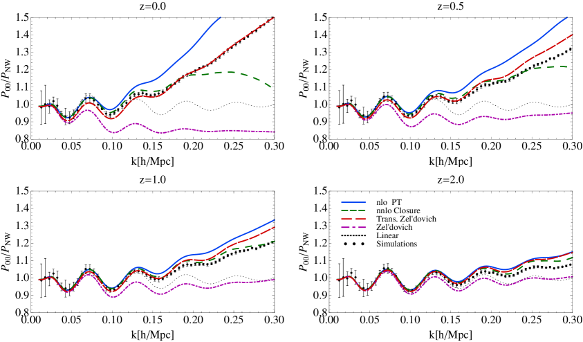
At the lowest order in expansion we have auto correlation of density field . Power spectrum, , is well known and has been intensively studied, e.g. [32, 17]. This first term does not have any dependence since it is independent of red shift space distortions, it dominants for small values of and in the limit the transverse power spectrum becomes overdensity power spectrum . On scales smaller than , nonlinear corrections increase the power over the linear.
Familiar one loop PT result for overdensity power spectrum is [17]
| (3.1) |
where we have restored time dependence, with being linear cosmological growth factor. is the linear power spectrum , and one loop contributions are
| (3.2) |
Explicit form of all integrals of the and type can be found in App D. In figure 1 one loop PT results for power spectrum have been presented, along with some of the other approaches, such as the closure theory approach [24] obtained from the Copter code [32] and the semi-fitting method [33], based on power spectrum obtained from Zel’dovich approximation. Note that if one wants to impose consistency in expansion 2.23 and PT approach, only one loop regime PT result should be considered. All the power spectra on the figures are divided by the linear power spectrum fitting formula from [34] without BAO wiggles. We see that none of the methods give perfect agreement across all range of scales. SPT (one loop PT) actually gives the best results for , but predicts too much power at higher .
3.2
The next term to consider correlates the overdensity field and radial component of momentum density . This is the dominant RSD term sensitive to velocities. As we can see from equation 2.16, momentum density can be decomposed into a scalar and two vector components . Only the scalar part correlates with the density , which is a scalar field. Thus only non-vanishing contribution comes from , what gives the simple angular dependence
| (3.3) |
On the other hand, correlating directly , from the equation 2.25 one gets power spectra
| (3.4) |
where the first term is also well studied correlation function of overdensity field and divergence of velocity field
| (3.5) |
For the first term, correlation function of overdensity and divergence of velocity field, one loop PT gives
| (3.6) |
where is the contribution in the linear regime, and one loop contribution is
| (3.7) |
Here we have introduced logarithmic growth rate
For the second term in equation 3.3, we expand all the fields to the second order, i.e., one loop in the correlation function. Schematically, this gives
or in terms of power spectrum
| (3.8) |
Again, using one loop PT we obtain the contributions from each of the terms
| (3.9) |
where the is the one-dimensional velocity dispersion at linear order, and . Note that all three terms give the same angular dependence, so , and then follows that , as was expected form the symmetry consideration on the beginning. Finally, collecting all the terms 3.4, 3.5, 3.8, 3.9 one loop PT prediction for the follows. Now the total contribution to the redshift power spectrum from the term is
| (3.10) |
In this form result is naturally separated in linear and one loop contribution part. Note that linear part here is the second term of Kaiser formula.
Alternatively, the scalar mode of momentum can be obtained from the divergence of momentum and related to using the continuity equation , which is in terms of quantities defined previously
| (3.11) |
Note that the vector part of momentum field does not contribute, since it vanishes upon taking the divergence (i.e., vector components are orthogonal to k and the dot product is zero).
It follows
| (3.12) |
and the total contribution to is
| (3.13) |
This result, first obtained in [28], is exact for dark matter, valid also in the nonlinear regime. It shows that this term can be obtained directly from the redshift evolution of the dark matter power spectrum , so if we have an accurate PT model for then we should also have the same for . On large scales it agrees with the linear theory predictions. If we write , we find Kaiser part . On smaller scales we expect the term to deviate from the linear one, just as for . Using one loop PT we simply need to calculate the derivatives of growth factor , and from equation 3.1 we get
| (3.14) |
Finely, plugging that in equation 3.13 we get
| (3.15) |
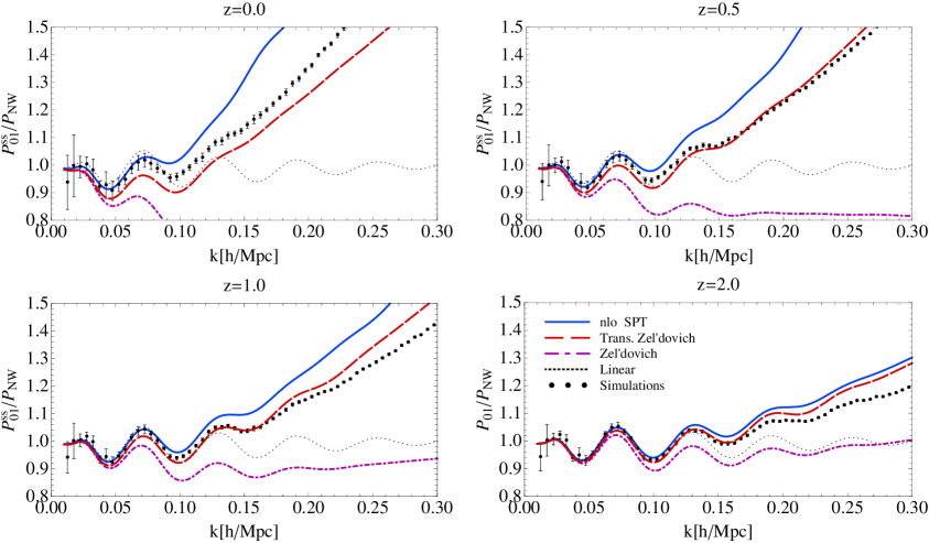
After some integral transformations and calculations it can be shown that this result is equivalent to the on in equation 3.10. Obtained results are presented in Figure 2. We show the one loop PT results, along with semi-fitting method [33] based on power spectrum in Zel’dovich approximation, and simulation measurements. The power spectra are now divided by second term in Kaiser formula where no-wiggle linear power spectrum has been used.
3.3
The next term we are to consider is the autocorrelation of momentum density field. In this case scalar correlates with itself, and the vector components also correlate with itself, so both components of momentum contribute,
| (3.16) |
Contributions to redshift space power spectrum is then given with
| (3.17) |
The scalar part is the autocorrelation of the of the momentum that contributes to the continuity equation 3.11. In linear PT only the scalar contribution in non-zero and , which is the last term in Kaiser formula. There is another contribution to both and terms from the vector part of momentum correlator , which comes in at the second order in power spectrum, and can be computed using one loop PT. This vector part is often called the vorticity part of the momentum, because vorticity of momentum does not vanish, even if vorticity of velocity vanishes for a single streamed fluid [35]. From equation 3.17 can be seen that this term always adds power to term and subtracts it in term, but is combined with a positive contribution from the scalar part in term.
Now using expressions 2.25 we can straightforwardly expand the correlator in density and velocity divergence fields. In terms of power spectra we have
| (3.18) |
where we have introduced:
| (3.19) |
Using one loop PT to evaluate these power spectra. First term gives familiar velocity divergence autocorrelation
| (3.20) |
where is the linear power spectrum and rest is one loop contribution to velocity divergence power spectrum ,
| (3.21) |
Second term can be expanded in the fields to the second order; schematically we have
This gives in terms of the power spectrum
| (3.22) |
where contributing terms are
| (3.23) |
Similarly, for the last term in equation 3.18, we have
| (3.24) |
Combining all that, we can write the contribution to redshift space power spectrum from term
| (3.25) |
As can be seen we obtained and angular dependence from this term, as was argued from symmetry consideration in [28]. Vector contribution can be identified as the part multiplying [28].
On the other hand, we could have started directly from equation 3.16. If we chose to work in the frame where one can write the decomposition 2.16 of momentum density , where we have chosen, without loss of generality, for to be in plane, and and represent scalar and vector part of decomposition, respectively. After averaging over angle, this enables us to write and . Just as before, scalar part can be determined directly from continuity equation 3.11. We can again use one loop PT to evaluate scalar and vector contributions
| (3.26) |
Thus, the contribution to the total red shift power spectrum from term is
| (3.27) |
Again, after some coordinate transformations and algebra it can be shown that this result is equivalent to the one we obtained earlier in equation 3.25.
In order to improve our prediction for the vector part we can take into consideration the most relevant higher order loop contributions. Starting from definition of (equation 3.19), which gives raise to the vector part of , and generalizing our one loop prediction in equation 3.24 we can write
| (3.28) |
In low limit this gives back the previous result from equation 3.24, and in high limit the first term dominates what is giving for the vector part.
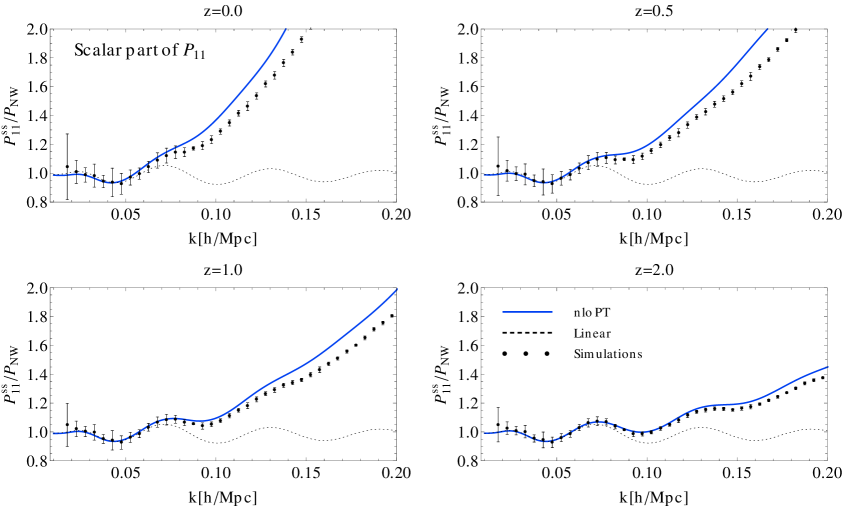
In figure 3 we show scalar part of which comes from scalar contributions. It has a simple angular dependence, and corresponds to the third Kaiser term. We divide the plots by this Kaiser limit, using the no-wiggle linear power spectrum. One loop PT results are compared to the simulation measurements. We see that PT is quite successful in reproducing the nonlinear evolution of this term.
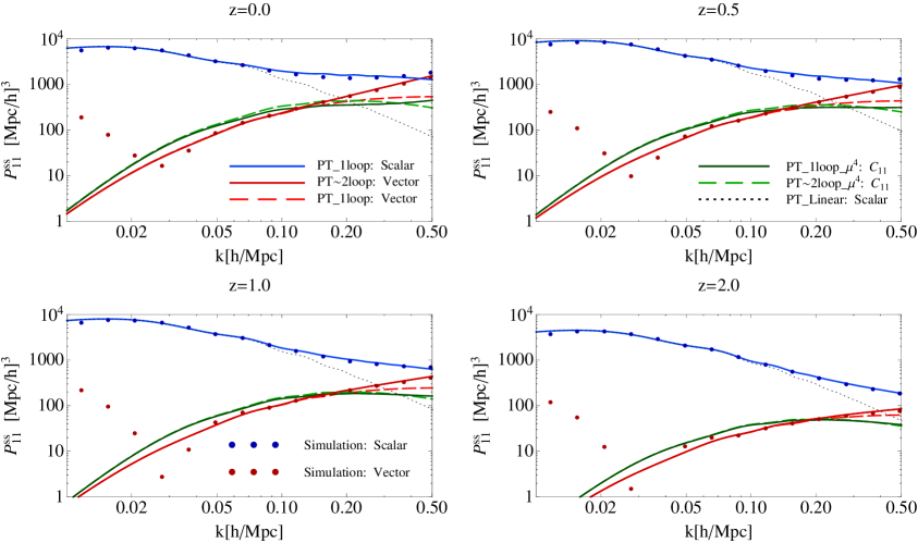
In figure 4 we show the vector part. We see that one loop PT is successful in reproducing the simulations for (the disagreement for is likely numerical), and adding two loop corrections increases these rage to larger . We also see that this vector contribution is considerably smaller than the scalar part for for most of the -range shown here, becoming comparable only at . However, because this vector term scales as while the linear scalar term scales as , the vector terms always dominates for sufficiently small . So for the nonlinear vector part exceeds linear scalar part already at .
3.4
At orders higher than there are no linear contributions, hence these terms are usually not of interest for extracting the cosmological information. However, these terms are known to be important on surprisingly large scales. These terms have usually been modeled phenomenologically in terms of adopting a simple functional form for and dependence and are related to the so called Fingers-of-God (FoG) effect. We begin with the dominant term, which, as we will see, is the last term to contribute to dependence.
We correlate the scalar density filed with the tensor field . Since scalars only correlate with scalars, there are only two different terms that contribute [28],
| (3.29) |
In terms of the contribution to the redshift space power spectrum this gives
| (3.30) |
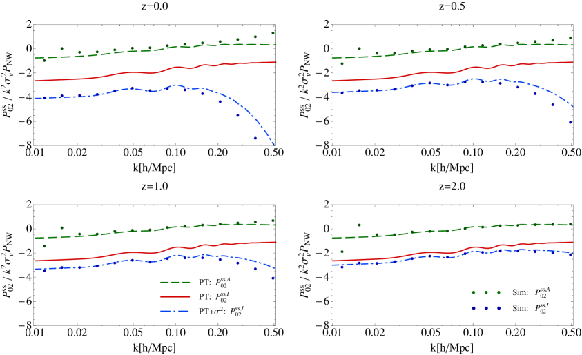
The first term is the correlation between the isotropic part of the mass weighted square of velocity, i.e. the energy density , and the density field , and the second term comes from the scalar part of the anisotropic stress , correlated with the density .
Before using PT to model these terms let us consider what we can expect from physical grounds. As argued in [28], in systems with a large rms velocity, the first, isotropic part should scale as , where has units of velocity square and includes the small scale velocity dispersion generated inside nonlinear halos. Some of this contribution cannot be modeled with simple fluid based PT, since not all of velocity dispersion is captured in this approach. As a result, we should not even hope that PT can be reliable for this term: we will need to add an extra contribution to account for the small scale velocity dispersion.
Expanding the fields we can write the contributing terms as following
| (3.31) |
where we have
| (3.32) |
Using the one loop PT to evaluate this terms we expand these terms in the following way
| (3.33) |
which after some computation give
| (3.34) |
Putting together all of the above we obtain for the contribution to the total redshift power spectrum
| (3.35) |
As we mentioned above, we have the contribution of form , which suppresses the linear power spectrum with a like effect, increasing towards higher . This is the lowest order FoG term, which we see contributes as and so effects the term of total . Because small scale velocity dispersion effects cannot be modeled by PT, which is restricted to the weakly non-linear regime, we will consider a model where we add to the PT predicted value for velocity dispersion the contributions coming from small scales. In the equations above we can then replace , where is the small scale addition to the velocity dispersion, and which we treat here as a free parameter. List of values used here for these parameters (depending on redshift), is given in the table 1, in section 3.8. In these section we also consider the explanation of these values using the halo model, see for example [36]. In addition to small scale velocity dispersion model, we also include the most relevant higher order PT terms. If we consider higher order contributions to term we see that it has subsets of diagrams where is not connected to any of the velocity fields, so we can write . Formally, in one loop computation only the leading term of this subset contributes in equation 3.34. Collecting these we see that we can model term by replacement
| (3.36) |
In order to discuss the results let us first rewrite equation 3.35 in form of isotropic and anisotropic part as for . We have , where
| (3.37) |
In figure 5 we show isotropic and anisotropic part of the contribution to the total redshift power spectrum. All power spectrum contributions are divided by the , where we again used the no-wiggle power spectrum. We can see that the contribution to is always negative, while the corresponding vector term from always adds power and the two partially cancel out [28]. As we see the scalar anisotropic stress-density correlator contributes to the angular term, as well as to the term. The anisotropic term is reasonably well modeled with PT and has smaller magnitude than the isotropic term, as expected, since the velocity dispersion in virialized objects is essentially isotropic. The isotropic term is poorly modeled with just PT: we need a significant contribution from the small scale velocity dispersion, which can be seen to essentially double the amplitude of this term at low , and far more than that at high . In figure 5 we can see that this term helps the model considerably, but of course it has one free parameter.
We can also write this result in powers of ,
| (3.38) |
where we have implicitly defined by omitting the velocity dispersion part from .
3.5
As we can see the lowest order in with which correlators contribute is the or . So contributions to comes only from terms , and . The next order in powers of will be terms. As we have seen and also have contributions to , with having the linear order term which dominates on large scales.
Here we correlate the momentum filed with the tensor field . Because of rotational invariance we can correlate only scalar to scalar field and vector to vector field
| (3.39) |
In terms of the contribution to the redshift space power spectrum this gives
| (3.40) |
Using the one loop PT we get both and angular terms, but since there are 3 terms we cannot distinguish between them in equation 3.40. Using equation 2.25 and one loop PT we get
| (3.41) |
where the contributing terms are
| (3.42) |
The first of these terms we can be expanded further
| (3.43) |
and computing these terms gives;
| (3.44) |
All this gives us the contribution to total redshift space power spectrum
| (3.45) |
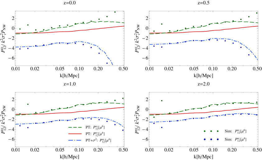
We can again add the small scale velocity dispersion in by hand, as was done and explained in case of . Considering the relevant higher order contributions we see that the isotropic part of can be modeled by
where we again treat small scale velocity dispersion as a free parameter with values for different redshifts given in table 1. These values are the same as for case, and the reasons and explanation in term of halo model is given in section 3.8.
As mentioned earlier, since we have only and angular dependence we can not determine all three terms in equation 3.40 separately. Let us instead separate the angular dependences itself and collect the terms
| (3.46) |
where we again implicitly define , by omitting the velocity dispersion part.
In figure 6 we show and parts to the total redshift power spectrum. Power spectrum contributions are divided by the , where we again used no-wiggle power spectrum.
3.6
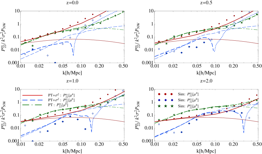
Next we consider correlator of tensor field with itself. This term will give , and contributions. One loop PT gives first order contributions to all of these angular terms. From the expansion of power spectrum 2.21 we can see that the constant contribution to is coming from the scalar term, and partially from and . This will give as the lowest order contribution to the total , and all of the other terms will come as , . Let us now assess these contributions using one loop PT
| (3.47) |
which gives rise to the total red shift power spectrum contribution
| (3.48) |
These are the leading order contributions to the angular dependence of this term. Now let us also investigate the most important contributions from the higher orders. For that purpose let us write the full correlator in terms of the density and velocity fields
| (3.49) |
In equation 3.48 we have considered only the first of these three terms, but we should also include some of the most important contributions from the remaining terms. From two loop considerations first we improve the first term 3.47 by exchanging linear power spectrum with one loop . The most important contributions of the other two terms can be modeled as
These are of course not the only higher order term, but after a detailed analysis these terms turn out to be the most relevant and the rest can be neglected. We can again include the small scale velocity dispersion extending as we did previously for and . Combining all we obtain a model
| (3.50) |
In high limit last (convolution) term corresponds to . In figure 7 we show the individual angular contributions for one loop PT calculus and for the improved model suggested above, and compare them to simulation measurements. We see that using the proposed model improves results in comparison to the one loop PT contributions, but still only qualitatively agrees with the simulations. One would find much better agreement if not imposing , i.e. with more free parameters. We mention that most of the correction to the term comes from the isotropic modeling of the last terms. Term also contributes to but less than the previous term. Corrections to the come from the angular dependency of term and we see that it can explain the change of sign and scale growth trends. The additional terms do not affect the term, which is well predicted (at least relative to and ) with two loop PT model of first term.
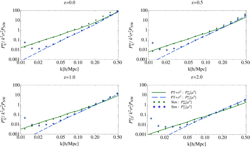
3.7 , and
Our goal is to consider all terms at the order. There are 3 left. First we consider terms and . We correlate overdensity field or momentum field with rank three tensor field . Angular decomposition for is relatively simple since it has only scalar contributions, but has scalar and vector contributions. Using the angular expansion we get the following angular dependence
| (3.51) |
In one loop PT these terms are
| (3.52) |
From angular decomposition of we have scalar terms, and , contributing with angular dependence and . One could evaluate these terms in PT, but at least two loop order is required for , since in one loop order gives just dependence. For we see that the lowest angular dependence comes from the vector contribution and not the scalar, although the scalar has lower perturbative order. Similar case was discussed for , where the vector part, which is of one loop order, contributes to , while the leading linear order scalar part has dependence.
One loop PT contribution to total give
| (3.53) |
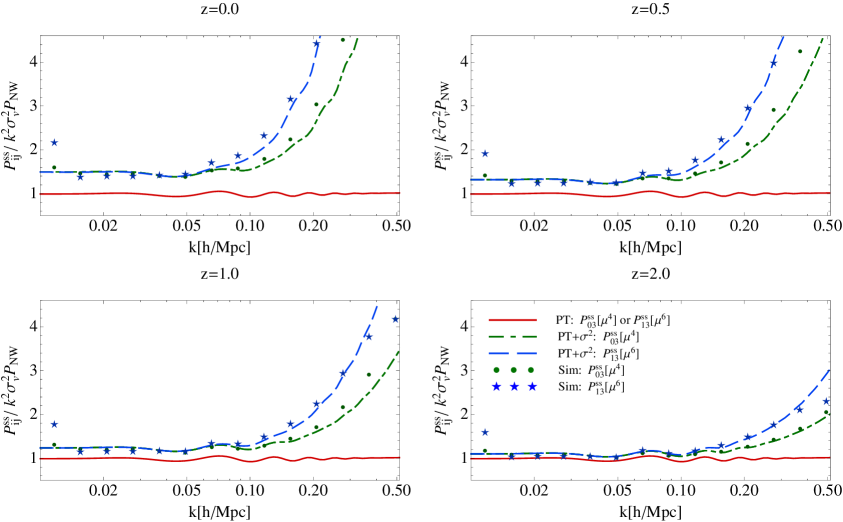
We can again include some higher order terms based on small scale velocity dispersion type arguments. For example, let us asses contributions to each of the terms above as if fully coming from
and neglecting other two loop contribution. Taking this into account we can model terms above by replacing and . In figure 8 we show results for both part of and for part of . On the same plot we show one loop PT prediction for both terms (keeping in mind that in the overall contribution they differ relative to each other by the factor of . We compare model results presented above to simulations. The specific shape in simulations is explained by the proposed model, while it is not in one loop PT result. This effect arises from substitution of with or . We can again add the small scale velocity dispersion (or equivalently ) which is not included in PT analysis. In the model we suggest for we get, in addition to the dependence, also dependence, which comes from the vector part of . In figure 9 we show that this can explain the trends and amplitude seen in simulations for this term. In the case of the leading contributions and we found that lower value for small scale velocity dispersion and is needed (table 1). This can be describer using the halo model and we return to that in section 3.8. Note that this value only affects the total amplitude, i.e. translates whole result up and down, but does not affect the shape.
In a similar fashion we can estimate contribution of term, which is the last term we need to consider at order. Formally this term does not even contribute at the one loop order in PT, but we can do two loop considerations as we did before. Considering the most relevant two loop contributions (from partially disconnected diagrams) this term can be modeled as
where we used subscript to label the connected part of the correlator. Here we again include the small scale velocity dispersion using , just as in case. We can write the contribution
| (3.54) |
3.8 Halo model and small scale velocity dispersion
In our analysis of correlators that contribute in expansion of the RSD power spectrum we find that some of them have terms proportional to velocity dispersion of dark matter particles. Particles moving in the gravitational potential can have large velocities even on the small scales, so they have significant contribution to the total velocity dispersion. Using PT we can evaluate velocity dispersion
| (3.55) |
Linear theory gives , but this does not properly take into account small scale contributions, which come from within virialized halos where PT cannot be used. Thus to take into account all nonlinear contributions we have to add this to our model in order to match the simulation predictions. In table 1 we show the values used for small scale velocity dispersion for modeled terms. These values are obtained by fitting our PT model using the free parameter for small scale dispersion () in order to match simulation predictions. We see that we can classify these into a few groups which have approximately the same value.
| z | 0.0 | 0.5 | 1.0 | 2.0 | z | 0.0 | 0.5 | 1.0 | 2. |
|---|---|---|---|---|---|---|---|---|---|
| , , (vector), | 375 | 356 | 282 | 144 | 377 | 267 | 190 | 105 | |
| , (scalar) | 209 | 198 | 159 | 80 | 221 | 154 | 106 | 56 | |
| 432 | 382 | 315 | 144 | 510 | 371 | 270 | 153 | ||
| 346 | 322 | 249 | 133 | 387 | 278 | 200 | 111 |
We can understand the fact that some terms have equal velocity dispersion to others, and some do not, using the halo model [37, 38, 36, 39, 40]. We can distinguish between three types of contributions to velocity dispersion. For terms and we find that the same value is needed. In these terms always comes weighted by . In a halo model we divide all the mass into halos, such that the integral over the halo mass function times mass gives the mean density of the universe,
| (3.56) |
where is halo mas function. Each halo has a bias , which describes how strongly the halo clusters relative to the mean, since
| (3.57) |
Each halo also has a small scale 1-d velocity dispersion , where the latter relation is only approximate and does not take into account effects such as halo profile dependence on the halo mass etc.
We now decompose the terms into halos of different mass, accounting for small scale velocity dispersion , and accounting for biasing whenever this is multiplied by density . For example for term schematically we can write
| (3.58) |
i.e. we find that the velocity dispersion is weighted by bias. Note that we should have written the term in halo model as well, but since the bias integrates to unity (equation 3.57) we do not have a contribution from the left hand side. Note also that we only include the small scale velocity dispersion effects here that come on top of the PT calculations above. Same quantity enters also in and .
For terms and we have a different contribution to small scale velocity dispersion because one of the velocity field in correlates with the density field and we can approximate with 1 at the lowest order. As a result is not density weighted. For example for we have contributions from term
| (3.59) |
Since there is no biasing and since at high mass halos which dominate the velocity dispersion these terms have a smaller value of velocity dispersion than we had in the first case. This is precisely what we find when fitting to the simulations.
Finally, for the term we find contribution
| (3.60) |
This term gives a value bigger then previous two because higher mass halos give a larger weight and they are more biased, which is also consistent with what we observe in simulations, and is presented in table 1. To convert into velocity dispersion we use the relation
| (3.61) |
see for example [41]. We use standard Sheth-Tormen model for halo mass function and halo bias [42]. We see that predictions from the halo model presented in 1 agree qualitatively but not quantitatively. This could be a consequence of the simplifying assumptions, such as ignoring the internal structure of the halo and its mass dependence. Note also that there are no errors in the analysis: it is possible that the sampling variance errors are large, specially for , which receives dominant contributions from the very high mass halos which may or may not be present in our simulations, depending on the realization. We do not go into a more detailed modeling here, but it is possible that with a more detailed model the agreement would improve. Even at this level the halo model gives an insight in hierarchy of the contributions , and offers a qualitative picture why different terms in expansion need different values for velocity dispersion.
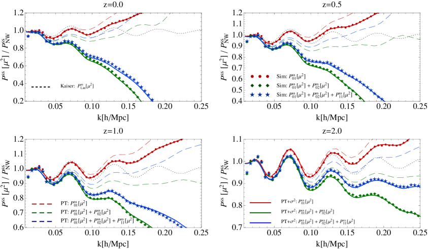
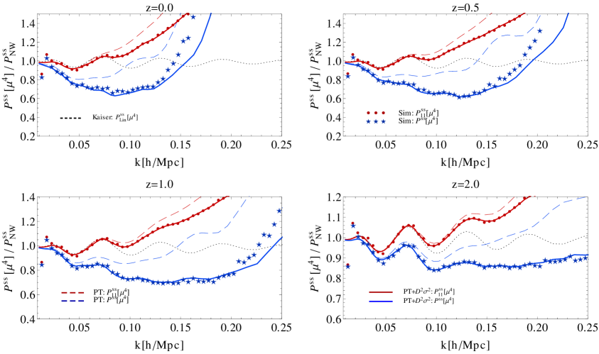
3.9 Putting it all together: terms, finger of god resummation and Legendre moments
There are a finite number of velocity moment terms at each order of , in contrast to the Legendre multipoles expansion (monopole, quadrupole, hexadecapole etc), which receive contributions from all orders in moments of distribution function. We will thus investigate expansion, with the lowest 3 orders containing cosmological information, while the rest can be treated as nuisance parameters to be marginalized over. Even in that case a good prior for these higher order angular terms would be very useful, although given the large number of terms that contribute to it it seems easier to be guided by the simulations rather than the PT. In this section we collect all the previous terms with and dependence. At level the contributions come from , and terms, and for from , , , , , and terms. In figures 10 and 11 we show and dependence of these terms divided by the corresponding no-wiggle Kaiser term. We show both the simplest PT model and the improved model that includes velocity dispersion effects. For modeling some of the terms we have been using the model for velocity dispersion , where the added value for term is given by the table 1. These model was optimized to fit corresponding terms primarily on large scales, where the dominant contributions comes from for and form terms. To improve the model further for and scalar part of , instead of PT predictions, we use exact values obtained from the simulations. We expect that ongoing activities in the modeling of nonlinear power spectrum will result in a successful model of these terms (note that is given by the time derivative of the nonlinear power spectrum ). Although we have introduced a free parameters in our model note that and terms do not contain any free parameters, so we can use simulation results as well as any other method to predict these terms.
The leading order in RSD is the term. On large scales it is given by the Kaiser expression, but note that the deviations from the linear theory are of the order of 10% at already at . These nonlinear effects are dominated by the small scale velocity dispersion effects, which cannot be modeled by PT (a smaller effect, of the order of 2% at these scales, is caused by nonlinear effects in which are modeled in PT). This is a serious challenge for the RSD models and the ability to extract cosmological information from RSD: any additional free parameter that needs to be determined from the data will reduce the statistical power of the data set. Note however that we do not observe dark matter, but galaxies, so to address this concern in a proper way one will need to repeat this study with galaxies. We plan to pursue this in the near future. At higher redshifts these nonlinear effects are smaller: at the 10% nonlinear suppression happens at . In all cases the dominant nonlinear effect is to suppress the small scale power, as expected by the phenomenological models like [9], where a Gaussian smoothing is added to the extension of Kaiser formula.
The terms show considerably more structure in the nonlinear effects: the overall power is initially suppressed relative to the linear term, stays flat for a while and then increases again (above at ). The effects are large: 20% suppression of power at for relative to linear. The model has some success in predicting some of these details, but is far from perfect and again it relies on the free parameters. The nonlinear effects are smaller at higher redshift, but remain significant. These terms have an important contribution to RSD. For example, at higher redshift (where ) they contribute about 30% to the quadrupole on large scales, with the dominant 70% contribution coming from term. As for the term, it remains to be seen how well we can model these terms such that we can extract the maximal information from the data, but the fact that the nonlinear effects are so large already on very large scales is a cause for concern.
Our result for the RSD power spectrum can be compactified in so called finger of good resummation. Following the ideas presented in [29] we can show explicitly that up to order our result in equation 2.23 can be written in the following way
| (3.62) |
where we have defined
| (3.63) |
i.e. there is no change to , and terms, since the terms and contain all the terms discussed previously and the FoG terms cancel by construction of and .
If we set the value of this reduces to simple form where is now present only in the exponent in equation 3.62 and not in the brackets, i.e.
| (3.64) |
where all the and terms here, as defined in previous sections, do not contain velocity dispersion contributions. This argument also generalizes to the case where we replace , where is the small scale velocity dispersion. This is the basic justification for using the FoG model.
Unfortunately, the fact that cancels out is of limited use, since in practice the velocity dispersion is not dominated by linear , but by small scale velocity dispersions, and as argued above, there is no single , but instead there are several different velocity dispersions entering in the detailed RSD analysis at and order, , and . In fact, in our analysis we include these terms already so one can argue that it is the next term that we do not include that should enter in . At order there are again several velocity dispersions that can be defined and that have a wide range of values, so we cannot simply write down a value without explicitly evaluating all the terms at this order. It is however likely that their values will be of the same order as , and . In table 1 we compare the root mean square average of these velocity dispersion values to the best fit value for , showing that indeed the value of is indeed related to these other values.
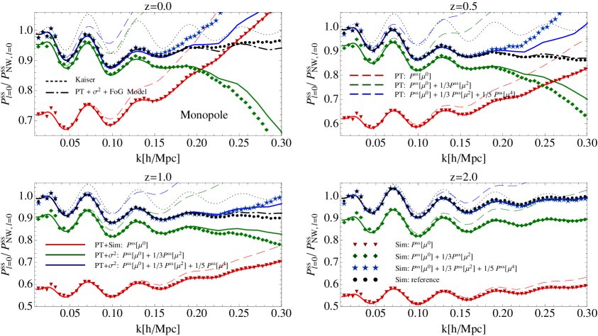
It is customary to expand the redshift-space power spectrum in terms of Legendre multipole moments. The motivation for this is that when using the full angular information Legendre moments are uncorrelated on scales small relative to the survey size. Using ordinary Legendre polynomials , we have
| (3.65) |
where multipole moments, , are given by
| (3.66) |
where are the ordinary Legendre polynomials, , and . In the RSD analyses we are usually limited to modeling the monopole () and quadrupole () terms, although some information is also contained in hexadecapole term ().
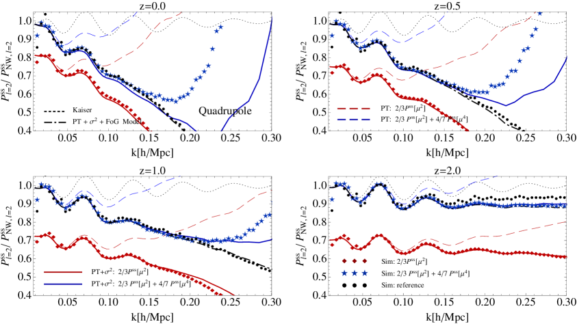
In figures 12 and 13 we show monopole and quadrupole power spectra predictions of improved velocity dispersion model presented in the paper, as well as one loop PT result. We also show resummed FoG result choosing for values given in the last line in table 1. We compare this to the reference multipole results obtained from full simulation redshift space power spectra. We also show simulation results where only terms up to are considered. In case of monopole we see that these two simulation results agree on scales larger then h/Mpc (depending on redshift) but then start to deviate one from an other. In the case of the quadrupole these deviations start to be more then 1% for h/Mpc. This trend is due to the term which is weighted by 1/7 for the monopole but 11/21 for the quadrupole, which is almost the same weight (4/7) as for term. At higher higher terms (, , …) start to be relevant and contribute significantly to the total redshift power spectrum. These higher contributions have large amplitudes with differing signs [29], which would suggest that we might not be able to rely on our expansion in low- any longer, although FoG resummation can still help here. From figures we can also see relative contributions to the total monopole and quadrupole power from and terms. We see that at scales larger than h/Mpc term contributes with 5-10% (depending on the redshift) to the total power of monopole and with 15-30% for the quadrupole. For the quadrupole all the remaining power comes form the term while for the monopole the term constitutes 25-35% of power and the rest comes from isotropic term. To reduce the dynamical range we again divide monopole results by the no-wiggle monopole Kaiser term and the quadrupole results by the no-wiggle quadrupole Kaiser term.
4 Conclusions
In this paper we use the distribution function approach to redshift space distortions (RSD) that decomposes RSD into moments of distribution function. Our goal is to model the terms that contribute to the redshift space distortions using perturbation theory. We first repeat the derivations presented in [28], explicitly deriving the decomposition of the moments into helicity eigenstates, based on their transformation properties under rotation around the direction of the Fourier mode. We give the explicit forms of correlators of the moments of distribution function and their angular dependencies.
It is worth comparing the phase space approach to the redshift space power spectrum to the alternative perturbative derivations that can be found in the literature, e.g. [21, 10]. The advantage of phase space approach as presented here lies in the decomposition into the hierarchy of terms that contribute to the redshift space power spectrum with an explicit dependence on the expansion parameters. In this way a systematic expansion approach is possible and a physical meaning of each term is revealed that enables effective modeling of each of the contributing correlators in the relation 2.19. This also allows a detailed term-by-term comparison of the simulation results, since one can compare each term to the simulations rather than just the final RSD power spectrum. In this paper we focus on the PT modeling and comparing the results to the simulations we are able to clearly show where the PT modeling preforms well, even at one loop, and where it does less so. The approach also allows us to identify physical reasons for failure of PT in individual terms, which are mostly related to various small scale velocity dispersion effects, and for which other modeling methods may be required. This also enables us to argue that it is more physical to try to model some of the terms in PT going beyond one loop, while remaining at the one loop level for the other terms. We should also mention that if just PT is used to evaluate all the terms at one loop, the results of phase space approach should correspond to [21], although only monopole predictions are presented there (compare e.g. figure 10 in [21] to SPT predictions for monopole in figure 12).
The leading order contributions to RSD can be classified in terms of their angular dependence, with the lowest order being and , where is the angle between the Fourier mode and the line of sight. There are three terms contributing to and seven terms contributing to . We evaluate all of these terms using the lowest order PT (one loop) and compare them to simulation results. For some terms adding two loop contributions proves to be important and we extend our models to include the relevant contributions. Also, for some of these terms standard PT is not sufficient and we propose physically motivated ansatz that goes beyond the loop analysis. These are based on the small scale induced velocity dispersion effects which multiply the long range correlations, such as density-density or density-velocity correlations. Such ansatz has a free parameter, small scale velocity dispersion, which cannot be modeled using PT. We found that a number of these terms have the same value, but also that not all velocity dispersions should be equal. We developed a halo model to describe the hierarchy of these terms and shown that the model can qualitatively explain the simulation results. Our analysis systematically accounts for all of the PT terms at one loop order and the small scale dispersion parameters, while necessary for a good description of RSD, have physically motivated values. In this sense our model goes beyond previous analyses [9, 10], which include some, but not all of the PT terms and which often treat FoG parameters as fitting parameters without a physical meaning.
The dominant term to RSD is the term and its dominant contribution is the momentum density correlated with the density. This term can be written in terms of a time derivative of the power spectrum [28] and so can be modeled using dark matter power spectrum emulators. Two other terms contribute to , the vector part of the momentum density-momentum density correlation, and the scalar part of energy density-density correlation. We find that they affect RSD at a 10% level already at . The energy density-density correlation term is the dominant nonlinear effect, is negative for all scales and thus reduces the total power. It is related to the Fingers-of-God effect. This term contains velocity dispersion term which cannot be modeled in PT and requires a free parameter in the model.
The next angular term has dependence and there are seven terms that contribute to the total power spectrum, of which one, scalar part of , contains a linear contribution that does not vanish on large scales. We evaluate all of these terms in PT. Some of these terms are well modeled by PT, while others also require velocity dispersion type parameters. With these the modeling achieves some level of precision compared to the simulations, but is still limited in the dynamic range, with an error of about 5% at at .
Our ultimate goal is to develop accurate models of RSD that can be applied to observations. We observe galaxies, not dark matter, and understanding the physical processes that lead to RSD in dark matter is just the first step towards the goal of understanding the RSD in galaxies. The results presented here are only a rough guide for the challenges awaiting us when applying these techniques to the data, but there are some lessons learned that are likely to be valid also for galaxies. One is the importance of velocity dispersion effects, which dominate our model uncertainties on large scales. The good news may be that the velocity dispersion effects, which are the main source of the modeling difficulties in this paper, may be smaller for galaxies than for the dark matter, specially if a sample of central galaxies can be selected. We also expect that the halo model for computing velocity dispersion should be applicable to galaxies as well. However, galaxies also have additional challenges not present for dark matter: galaxy biasing will introduce additional scale dependent effects in redshift space that will need to be modeled, even if there are no such scale dependent biases in real space [28, 43]. The success of modeling the RSD and extracting the cosmological information from it depends on our ability to model these galaxy biasing and velocity dispersion terms. We plan to address some of these issues in the future work.
Acknowledgments
We would like to thank Nico Hamaus, Darren Reed and Lucas Lombriser for useful discussions and comments. ZV would like to thank the Berkeley Center for Cosmological Physics and the Lawrence Berkeley Laboratory for their hospitality. This work is supported by the DOE, the Swiss National Foundation under contract 200021-116696/1 and WCU grant R32-10130. The simulations were performed on the ZBOX3 supercomputer of the Institute for Theoretical Physics at the University of Zürich.
Appendix A Components of moments of distribution function
Starting from equation 2.6 we can chose some basis, for example Cartesian, to express scalar product . It follows
| (A.1) |
where summation over is implied. Using the multinomial theorem:
| (A.2) |
it follows that
| (A.3) |
Neglecting velocity dispersion and anisotropic stress second rank tensor, and similar higher rank tensors contributions () we are left with
| (A.4) |
where is given in equation 2.4. Returning this back into equation A.3 and using multinomial theorem again we get
| (A.5) |
Thus we have retrieved result of equation 2.7, and choosing we get equation 2.13.
Appendix B Decomposition of in spherical tensors
In this section we want to retrieve, starting from equation 2.15, equation 2.16. Let us consider the object as defined in 2.6, which can actually be constructed by contracting all the components of rank of tensor (equation 2.15) with unit h vectors. Fourier transforming this object gives us simply
| (B.1) |
Since we have translation symmetry it follows
where it is implied that we take correlation of a general function of similar form like equation 2.6. This enables us to work with each Fourier mode separately, and add them appropriately in the end when we discuss the power spectrum. By symmetry of the problem we may choose a reference frame where -axis is along h vector. Since spherical harmonics form a complete set of orthonormal functions and thus form an orthonormal basis of the Hilbert space of square-integrable functions, we can expanded in that frame as a linear combination,
| (B.2) |
where is the amplitude of momentum. Let us now consider the transformation properties of under rotation around the -axis. We can think of rotation by some angle (i.e. ) in two ways
From rotation properties of spherical harmonics it follows that transform as
| (B.3) |
so it is an eigenstate of an helicity operator , with helicity eigenvalue, or simply helicity, . A quantity with helicity 0 is called a scalar, that with helicity is called a vector and that with a tensor, but the expansion goes to arbitrary values of . It is possible to do similar considerations for arbitrary rotation and so it can be shown that transform as spherical tensors.
In the chosen reference frame, using , and inserting equation B.2 into equation B.1 we obtain
| (B.4) |
where we have defined helicity eigenstates of moments of the distribution function
| (B.5) |
and used abbreviation for the integral
| (B.6) |
We have used definition of spherical harmonics , and abbreviation. Since in equation B.4 we have Kronecker delta it is easy to evaluate integral
| (B.7) |
and here we have used . Collecting all that, equation B.4 becomes
| (B.8) |
Since we are working in frame it is apparent that for some arbitrary k, the angular dependence is contained in spherical tensors. The goal now is to disentangle the angular dependence from the radial. The procedure depends on whether one is using active or passive interpretation of rotation transformation. Let us first look at active interpretation. Then the completely contracted tensors, like the one we are dealing with equation B.8, can be obtained from the same one evaluated in direction by rotating it in general k direction. Because are spherical tensors it follows
| (B.9) |
where is the Wigner rotation matrix and its matrix elements. Using the well known relations, and , we get
| (B.10) |
where spherical harmonics now describe rotation form direction k back to h. On the other hand, using the passive interpretation we argue that in frame can be obtained by rotating it from frame, which is described by the same equations as before B.9. Note now that we were able to express result in terms of , just a function of amplitude , and all angular dependence is given with spherical harmonics which now describe the angular dependence in h direction seen from frame. Now setting simply along a line of sight direction we get result 2.16, where .
Appendix C Conjugation properties of
In this section we investigate the conjugation properties of functions. Starting from the condition that overdensity field and velocity field are real valued fields, it follows that for Fourier space fields , and we have . This is valid also for more complex fields like
| (C.1) |
If we compute conjugated field we get
| (C.2) |
From equation 2.7 it follows that , so for correlator we have
| (C.3) |
thus we have . So, for sum of two correlator we can write
| (C.4) |
Appendix D Integrals and
Here we define integrals and used in previous chapters:
| (D.1) |
where we define kernels , and use and :
| , | , |
| , | , |
| , | , |
| , | , |
| , | , |
| , | , |
| , | , |
| , | . |
Also we have kernels :
| (D.2) |
and all the rest vanish in next to leading order regime.
References
- [1] N. Kaiser, Clustering in real space and in redshift space, Mon. Not. Roy. Astron. Soc. 227 (1987) 1–27.
- [2] A. Hamilton, Linear redshift distortions: A Review, astro-ph/9708102. Published in The Evolving Universe. Edited by D. Hamilton, Kluwer Academic, 1998, p. 185-275.
- [3] S. Cole, K. B. Fisher, and D. H. Weinberg, Fourier analysis of redshift space distortions and the determination of Omega, Mon.Not.Roy.Astron.Soc. 267 (1994) 785, [astro-ph/9308003].
- [4] M. White, Y.-S. Song, and W. J. Percival, Forecasting Cosmological Constraints from Redshift Surveys, Mon.Not.Roy.Astron.Soc. 397 (2008) 1348–1354, [arXiv:0810.1518].
- [5] P. McDonald and U. Seljak, How to measure redshift-space distortions without sample variance, JCAP 0910 (2009) 007, [arXiv:0810.0323]. * Brief entry *.
- [6] G. M. Bernstein and Y.-C. Cai, Cosmology without cosmic variance, arXiv:1104.3862.
- [7] A. Amara and A. Refregier, Optimal Surveys for Weak Lensing Tomography, Mon.Not.Roy.Astron.Soc. 381 (2007) 1018–1026, [astro-ph/0610127].
- [8] L. Casarini, S. A. Bonometto, S. Borgani, K. Dolag, G. Murante, et. al., Tomographic weak lensing shear spectra from large N-body and hydrodynamical simulations, arXiv:1203.5251.
- [9] R. Scoccimarro, Redshift-space distortions, pairwise velocities and nonlinearities, Phys.Rev. D70 (2004) 083007, [astro-ph/0407214].
- [10] A. Taruya, T. Nishimichi, and S. Saito, Baryon Acoustic Oscillations in 2D: Modeling Redshift-space Power Spectrum from Perturbation Theory, Phys.Rev. D82 (2010) 063522, [arXiv:1006.0699].
- [11] E. Jennings, C. M. Baugh, and S. Pascoli, Modelling redshift space distortions in hierarchical cosmologies, Mon.Not.Roy.Astron.Soc. 410 (2011) 2081, [arXiv:1003.4282].
- [12] J. Tang, I. Kayo, and M. Takada, Likelihood reconstruction method of real-space density and velocity power spectra from a redshift galaxy survey, arXiv:1103.3614.
- [13] J. L. Tinker, Redshift-Space Distortions with the Halo Occupation Distribution II: Analytic Model, Mon.Not.Roy.Astron.Soc. 374 (2007) 477–492, [astro-ph/0604217].
- [14] T. Nishimichi and A. Taruya, Baryon Acoustic Oscillations in 2D II: Redshift-space halo clustering in N-body simulations, Phys.Rev. D84 (2011) 043526, [arXiv:1106.4562].
- [15] B. A. Reid and M. White, Towards an accurate model of the redshift space clustering of halos in the quasilinear regime, arXiv:1105.4165.
- [16] M. Sato and T. Matsubara, Nonlinear Biasing and Redshift-Space Distortions in Lagrangian Resummation Theory and N-body Simulations, Phys.Rev. D84 (2011) 043501, [arXiv:1105.5007].
- [17] F. Bernardeau, S. Colombi, E. Gaztanaga, and R. Scoccimarro, Large scale structure of the universe and cosmological perturbation theory, Phys.Rept. 367 (2002) 1–248, [astro-ph/0112551].
- [18] M. Crocce and R. Scoccimarro, Renormalized cosmological perturbation theory, Phys.Rev. D73 (2006) 063519, [astro-ph/0509418].
- [19] M. Crocce and R. Scoccimarro, Memory of initial conditions in gravitational clustering, Phys.Rev. D73 (2006) 063520, [astro-ph/0509419].
- [20] M. Crocce and R. Scoccimarro, Nonlinear Evolution of Baryon Acoustic Oscillations, Phys.Rev. D77 (2008) 023533, [arXiv:0704.2783].
- [21] T. Matsubara, Resumming Cosmological Perturbations via the Lagrangian Picture: One-loop Results in Real Space and in Redshift Space, Phys.Rev. D77 (2008) 063530, [arXiv:0711.2521].
- [22] T. Matsubara, Nonlinear perturbation theory with halo bias and redshift-space distortions via the Lagrangian picture, Phys.Rev. D78 (2008) 083519, [arXiv:0807.1733].
- [23] P. McDonald, Dark matter clustering: a simple renormalization group approach, Phys.Rev. D75 (2007) 043514, [astro-ph/0606028].
- [24] A. Taruya and T. Hiramatsu, A Closure Theory for Non-linear Evolution of Cosmological Power Spectra, arXiv:0708.1367.
- [25] M. Pietroni, Flowing with Time: a New Approach to Nonlinear Cosmological Perturbations, JCAP 0810 (2008) 036, [arXiv:0806.0971].
- [26] P. Valageas, A new approach to gravitational clustering: a path-integral formalism and large-n expansions, Astron.Astrophys. 421 (2004) 23–40, [astro-ph/0307008].
- [27] A. Taruya, T. Nishimichi, S. Saito, and T. Hiramatsu, Non-linear Evolution of Baryon Acoustic Oscillations from Improved Perturbation Theory in Real and Redshift Spaces, Phys.Rev. D80 (2009) 123503, [arXiv:0906.0507].
- [28] U. Seljak and P. McDonald, Distribution function approach to redshift space distortions, arXiv:1109.1888.
- [29] T. Okumura, U. Seljak, P. McDonald, and V. Desjacques, Distribution function approach to redshift space distortions: N-body simulations, arXiv:1109.1609.
- [30] P. J. E. Peebles, Principles of physical cosmology, . Princeton, USA: Univ. Pr. (1993) 718 p.
- [31] V. Desjacques, U. Seljak, and I. Iliev, Scale-dependent bias induced by local non-Gaussianity: A comparison to N-body simulations, arXiv:0811.2748.
- [32] J. Carlson, M. White, and N. Padmanabhan, A critical look at cosmological perturbation theory techniques, Phys. Rev. D80 (2009) 043531, [arXiv:0905.0479].
- [33] S. Tassev and M. Zaldarriaga, The Mildly Non-Linear Regime of Structure Formation, arXiv:1109.4939.
- [34] D. J. Eisenstein and W. Hu, Baryonic Features in the Matter Transfer Function, Astrophys. J. 496 (1998) 605, [astro-ph/9709112].
- [35] P. McDonald, How to generate a significant effective temperature for cold dark matter, from first principles, JCAP 1104 (2011) 032, [arXiv:0910.1002].
- [36] U. Seljak, Analytic model for galaxy and dark matter clustering, Mon.Not.Roy.Astron.Soc. 318 (2000) 203, [astro-ph/0001493].
- [37] J. Peacock and R. Smith, Halo occupation numbers and galaxy bias, Mon.Not.Roy.Astron.Soc. 318 (2000) 1144, [astro-ph/0005010].
- [38] C.-P. Ma and J. N. Fry, What does it take to stabilize gravitational clustering?, astro-ph/0005233.
- [39] A. A. Berlind, D. H. Weinberg, A. J. Benson, C. M. Baugh, S. Cole, et. al., The Halo occupation distribution and the physics of galaxy formation, Astrophys.J. 593 (2003) 1–25, [astro-ph/0212357].
- [40] A. Cooray and R. K. Sheth, Halo models of large scale structure, Phys.Rept. 372 (2002) 1–129, [astro-ph/0206508].
- [41] U. Seljak, Constraints on galaxy halo profiles from galaxy-galaxy lensing and tully-fisher/fundamental plane relations, Mon.Not.Roy.Astron.Soc. 334 (2002) 797, [astro-ph/0201450].
- [42] R. K. Sheth and G. Tormen, Large scale bias and the peak background split, Mon.Not.Roy.Astron.Soc. 308 (1999) 119, [astro-ph/9901122].
- [43] T. Okumura, U. Seljak, and V. Desjacques, Distribution function approach to redshift space distortions, Part III: halos and galaxies, arXiv:1206.4070.