Magnetohydrodynamic stability of broad line region clouds

Abstract

Hydrodynamic stability has been a longstanding issue for the cloud model of the broad line region in active galactic nuclei. We argue that the clouds may be gravitationally bound to the supermassive black hole. If true, stabilisation by thermal pressure alone becomes even more difficult. We further argue that if magnetic fields should be present in such clouds at a level that could affect the stability properties, they need to be strong enough to compete with the radiation pressure on the cloud. This would imply magnetic field values of a few Gauss for a sample of Active Galactic Nuclei we draw from the literature.

We then investigate the effect of several magnetic configurations on cloud stability in axisymmetric magnetohydrodynamic simulations. For a purely azimuthal magnetic field which provides the dominant pressure support, the cloud first gets compressed by the opposing radiative and gravitational forces. The pressure inside the cloud then increases, and it expands vertically. Kelvin-Helmholtz and column density instability lead to a filamentary fragmentation of the cloud. This radiative dispersion continues until the cloud is shredded down to the resolution level. For a helical magnetic field configuration, a much more stable cloud core survives with a stationary density histogram which takes the form of a power law. Our simulated clouds develop sub-Alfvénic internal motions on the level of a few hundred km/s.

1 Introduction

Broad emission lines are produced in the immediate vicinity of optically active super-massive black holes (SMBH, for reviews see e.g. Osterbrock 1988; Peterson 1997; Netzer 2008). They may be used to infer the black hole mass in galaxies with such an Active Galactic Nucleus (AGN, e.g. Bentz et al. 2009), and are a standard part of optically active AGN. The basic line emitting entity is usually referred to as a cloud. The emission mechanism is photoionisation by the central parts of the accretion disc. Photoionisation models predict the clouds to have a typical temperature of order $10^{4}$ K, number densities of $n_{\mathrm{cl}}=10^{10\pm 1}$ cm^-3, sizes of $R_{\mathrm{cl}}=10^{12\pm 1}$ cm and column densities of $N_{\mathrm{cl}}>2\times 10^{22}$ cm^-2 (e.g. Kwan & Krolik 1981; Ferland & Elitzur 1984; Rees et al. 1989). Further important constraints come from reverberation mapping (e.g. Peterson 1988, see below for a comparison of results of these two methods). The complete physics of these clouds is however highly complex and involves also pressure, radiative, centrifugal, gravitational, and magnetic forces, probably on a very similar level. We are not aware of any attempt to include all these processes into a single model, but different authors have looked at some particular aspects of the problem: A general assumption for the cloud ensemble is often virial equilibrium. Since the gravitational potential is dominated by the SMBH, this would imply Kepler orbits. This treatment neglects the contribution of radiation pressure to the dynamics. The latter restriction has been relaxed in a recent series of papers (Marconi et al. 2008, 2009; Netzer 2009, 2010; Krause, Burkert, & Schartmann 2011 (hereafter: paper I)). The general finding is that the radiation force may contribute significantly, and that in this case, the clouds on bound orbits could be significantly sub-Keplerian. For low angular momentum (strong radiation pressure support), the orbits have to be highly excentric.

The importance of radiation pressure has actually been recognised early on (e.g. Tarter & McKee 1973; McKee & Tarter 1975; Blumenthal & Mathews 1975, 1979; Mathews 1976). In fact, many of the earlier articles study the possibility that radiation pressure is dominant, also compared to gravity, and the clouds are unbound. In this case, it would however not be easy to understand why the black hole masses derived from reverberation mapping under the assumption of virial equilibrium may be brought into agreement with the correlation between black hole mass and host galaxy properties with a uniform scaling factor (Onken et al. 2004). For optically thin clouds, one would expect almost no response to the variability of the ionising continuum. The strong variability of the emission lines, lead by variations in the continuum is therefore evidence for the presence of optically thick clouds (e.g. Snedden & Gaskell 2007). However, the relative importance of gravity versus radiation pressure is proportional to the optical thickness (compare equation (3), below).
This opened up the possibility that the Broad Line Region (BLR) is gravitationally bound and possibly disc-like with a significant total angular momentum. In fact, several pieces of evidence that point in this direction have been found over recent years (compare paper I and references therein). One recent piece of evidence comes from spectropolarimetry, where the BLR is spatially resolved by an equatorial scattering region, leading to different polarisation angles in the red and blue wings of emission lines (Smith et al. 2005). Most recently, Kollatschny & Zetzl (2011) have shown that the shape of the broad emission lines in many objects may be well fit with the assumption of a turbulent thick disc.

Cloud stability and confinement is a long-standing issue (Osterbrock & Mathews 1986, for a review): The clouds should be in rough pressure equilibrium with their environment (e.g. Krolik, McKee, & Tarter 1981; Krolik 1988). To reach the required pressure of $p\approx 10^{-2}$ dyne cm^-2, the inter-cloud medium needs either a high temperature ($>4\times 10^{7}$ K, Krolik 1988) or a strong magnetic field (Rees 1987). Apart from the confinement issue, the clouds should be hydrodynamically unstable: Mathews (1982) has shown that while optically thin clouds may be close to uniformly accelerated by the radiation pressure, there remain internal radial pressure imbalances, which especially in the optically thick case, which is preferred by photoionisation models, lead to lateral expansion of the clouds. He termed the latter state pancake clouds. Mathews (1986) then assessed the hydrodynamic stability of such pancake clouds with the result that the lateral edges of a pancake cloud are hydrodynamically unstable. Hence, the lateral flows persist and destroy the cloud on a short timescale, comparable to one cloud orbit. Also, the ram pressure by the inter-cloud gas, which is probably pressure supported and moving in a different way than the clouds, may compress the clouds in the direction of relative motion and the increased pressure makes the clouds expand sideways (Krolik 1988), now with regard to the direction of motion. These problems have lead to the idea that clouds must reform or be re-injected steadily. Krolik (1988) develops the idea of clouds forming by the thermal instability from the hot inter-cloud gas. This idea has however been rejected by Mathews & Doane (1990): It would require very large amplitude fluctuations of unusual type (high density, low temperature). Additionally, a compression by a factor of 10,000 would require an unusually small magnetic field, for the magnetic pressure not to stop the collapse. Mathews & Doane (1990) further argue that the clouds would be destroyed by the radiative shear mechanism before they could contribute to the emission line profiles. We have studied the radiative shearing mechanism for dusty clouds in 2.5D hydrodynamic simulations (Schartmann et al. 2011). In agreement with Mathews (1986) and Mathews & Doane (1990), we find quick radiative shearing of the cloud.

As mentioned above, the stability considerations were for clouds accelerating due to the dominant radiation pressure. The problem is even more severe for bound clouds where gravity is comparable to the radiation force: The radiation force acts on the illuminated surface of the cloud, while every part of the cloud is uniformly subject to gravity which must dominate by definition for bound clouds. Such clouds are therefore compressed, and must consequently be stabilised by some internal pressure. Yet, radiation pressure and gravity act in one dimension, whereas the thermal pressure is isotropic. It is therefore not possible to stabilise illuminated bound clouds by thermal pressure alone.

In this context, we investigate the stability of magnetised and gravitationally bound BLR clouds – initially close to an equilibrium orbit as calculated in paper I. Magnetic fields have so far rarely been considered in BLR clouds. We therefore first review literature data for indications on the relative magnitudes of gravitational, magnetic and radiative forces. (section 2). We then focus on the effect of the magnetic field, and simulate the evolution of irradiated magnetically dominated bound clouds. We study the two-dimensional, axisymmetric (2.5D), magnetohydrodynamic (MHD) evolution of isolated, initially optically thick clouds, including gravity, rotation and radial radiation pressure via a simple equilibrium photoionisation ansatz. We neglect self-gravity, viscosity and any radiation source other than the central accretion disc. Because of the small size of the clouds, our computational domain is small compared to the full size of the BLR. We describe technical details in section 3, the setup details in section 4, our results in section 5 and discuss our findings in section 6. We summarise our results in section 7.

2 Magnetic fields, gravity and radiation pressure in BLR clouds – indications from the literature

The typical pressure level imposed on the clouds by radiative, and gravitational forces may be calculated from reverberation mapping (RM) data as follows: For this analysis we convert all forces to pressures, dividing by the surface area of the cloud, assumed to be spherical in this order of magnitude analysis. The inwards pressure due to gravity on the cloud is given by:

$$p_{\mathrm{G}}=\frac{GM_{\mathrm{BH}}m_{\mathrm{cld}}}{r^{2}}\frac{1}{\pi R_{\mathrm{cld}}^{2}}\,,$$ (1)

where $M_{\mathrm{BH}}$ is the black hole mass, $m_{\mathrm{cld}}$ the mass of the cloud, $r$ the distance of the cloud from the black hole, and $R_{\mathrm{cld}}$ the radius of the cloud. In current reverberation mapping studies (e.g. Bentz et al. 2009), the black hole mass is determined as a function of the measured quantities of the centroid time lag $\tau_{\mathrm{cent}}$ and the line dispersion of the rest frame rms-spectra, $\sigma_{\mathrm{line}}$. Using these variables, the gravitational pressure on the clouds may be expressed as:

$$p_{\mathrm{G}}=\frac{4}{3}f\frac{R_{\mathrm{cld}}}{c\tau_{\mathrm{cent}}}\rho_{\mathrm{cld}}\sigma_{\mathrm{line}}^{2}\,.$$ (2)

Here, $\rho_{\mathrm{cld}}$ is the density of the clouds, and $f=5.5$ is the correction factor which ensures that RM-based black hole masses agree with the $M_{\mathrm{BH}}$–$\sigma_{*}$ relation (Onken et al. 2004). We have collected $\tau_{\mathrm{cent}}$ and $\sigma_{\mathrm{line}}$ from a number of RM-studies where they were explicitly stated (Table 1). Where available, we have included different measurements of the same source at different epochs. From this data we have calculated $p_{\mathrm{G}}$ using $R_{\mathrm{cld}}\rho_{\mathrm{cld}}=0.23$ g cm^-2 (corresponding to a hydrogen column density of $N_{H}=10^{23}$ cm^-2), which is plotted against black hole mass in Figure 1 (top). The values for $R_{\mathrm{cld}}$ and $\rho_{\mathrm{cld}}$ are chosen to be in the range allowed from photoionisation models (compare section 1). There seems to be no obvious correlation. The mean of the gravitational pressure in the clouds is 3.63 dyne/cm². Because the distribution seems to be more uniform in log-space, we use in the following the median value, which is 1.75 dyne/cm², as a characteristic number.

The ratio between radiation pressure and gravitational pressure may be expressed as:

$$\frac{p_{\mathrm{R}}}{p_{\mathrm{G}}}=\frac{3}{16\pi cG}\frac{1}{R_{\mathrm{cld}}\rho_{\mathrm{cld}}}\frac{L_{\mathrm{ion}}}{M_{\mathrm{BH}}}\,,$$ (3)

where $L_{\mathrm{ion}}$ is that part of the AGN light that is absorbed by the cloud. It is given by (e.g. Marconi et al. 2008) $L_{\mathrm{ion}}=abcL_{5100}$, where $a=0.6$ is the ionising fraction of the bolometric luminosity, $b=9$ is the bolometric correction and $L_{5100}$ represents $\lambda L_{\lambda}$ at 5100 Å.

The factor $c$ accounts for geometrical and relativistic effects: Sun & Malkan (1989) have shown that for frequencies up to about $\nu=10^{15}$ Hz, the angular radiation pattern of thin accretion discs around fast rotating black holes follow the classical $\cos(\theta)$-law (Lambert’s law). For $\nu\gtrsim 10^{16}$ Hz, the emission is close to isotropic. For Schwarzschild black holes, the transition occurs at somewhat higher frequencies. Luminous AGN emit most of their energy in the innermost regions of the accretion disc, in the blue – ultraviolet part of the spectrum (so-called “big blue bump”), with a peak around $\nu_{\mathrm{p}}=2\times 10^{15}$ Hz (e.g. Hopkins, Richards, & Hernquist 2007). If Lambert’s law would apply and if the BLR would extend 20 degrees above and below the equatorial plane, which would mean that about 10 per cent of the AGN’s radiation would be intercepted, $c$ would average to 0.3. For more rapidly spinning black holes or accretion discs emitting at higher frequencies, $c$ might become as large as unity. Also, if the BLR would not be located in the equatorial plane of the accretion disc, $c$ would also tend towards unity. Here, we adopt $c=1$ as possible, reasonable value.

For these assumptions, we have calculated the pressure ratio for the sample of Peterson et al. (2004) (their complete Table 8). We have used this sample, because black hole masses determined in the same way as for the sample above as well as continuum luminosities were available. We show a plot of the derived pressure ratios against black hole mass in Figure 1 (bottom). There is again no obvious correlation. The mean ratio of radiation to gravitational pressure is 0.74. Here, the distribution is also more uniform in log-space, and therefore again we use the median of the pressure ratios as a characteristic number, which is 0.48. These numbers depend of course crucially on the assumed column density. Photoionisation calculations constrain the column density to $N>2\times 10^{22}$cm^-2 (Kwan & Krolik 1981). We have used values for $R_{\mathrm{cld}}$ and $\rho_{\mathrm{cld}}$ corresponding to a (hydrogen) column of $N=10^{23}$cm^-2, consistent with the requirement from reverberation mapping studies that the clouds need to be optically thick (compare section 1, above). Allowing for the smallest column density consistent with the calculations of Kwan & Krolik (1981) would shift the median of the pressure ratio to 2.39, with only 6 of 35 values still below unity. However, Maiolino et al. (2010) and Risaliti et al. (2011) have possibly observed BLR clouds in X-ray absorption and give values of a few times $10^{23}$ for the column of their clouds. With such a column density, the typical pressure ratio would clearly drop below unity. We have included a contribution of 80 per cent due to the uncertainties in the column density for the calculation of the error bars in Figure 1. Another uncertainty is due to the accuracy of the black hole masses: As indication, the errors stated by Bentz et al. (2009, their Table 13) are 43 per cent. Additionally, there may be a systematic error via $f$ (Onken et al. 2004), and possibly corrections to radiation pressure (Marconi et al. 2008, 2009). Because the pressure ratio values we find scatter around unity (Figure 1), it is thus not possible to firmly conclude if the BLRs are typically gravitationally bound or otherwise. It is however remarkable that the pressure ratio distribution is bounded by a value close to unity for reasonable assumptions. In any case, gravitationally bound cloud models are clearly consistent with the data.

Figure 1: Radial pressure on BLR clouds. Top: Inwards pressure due to gravity over black hole mass (data of Table 1). Bottom: ratio of radiative to gravitational pressure (all 35 objects of Peterson et al. 2004). Different samples have been used for each plot, according to the availability of the data. Error bars are propagated from the original publications (compare Table 1). Additionally, an error of 80 per cent on the assumed column density has been included. See text for details.

Table 1: Reverberation mapping data

Object	$\tau_{\mathrm{cent}}$	$\Delta\tau_{\mathrm{cent}}$	$\sigma_{\mathrm{line}}$	$\Delta\sigma_{\mathrm{line}}$
	(days)	(days)	(km/s)	(km/s)
Bentz et al. (2009)
Mrk142	2.74	0.75	859	102
SBS1116+583A	2.31	0.56	1528	184
Arp151	3.99	0.59	1252	46
Mrk1310	3.66	0.60	755	138
Mrk202	3.05	1.43	659	65
NGC4253	6.16	1.43	516	218
NGC4748	5.55	1.92	657	91
NGC5548	4.18	1.08	4270	292
NGC6814	6.64	0.89	1610	108
Denney et al. (2009)
NGC4051	1.87	0.52	927	64
Grier et al. (2008)
PG2130+099	22.9	4.7	1246	222
Denney et al. (2006)
NGC4593	3.73	0.75	1561	55
Bentz et al. (2007)
NGC5548	6.3	2.5	2939	768
Bentz et al. (2006)
NGC5548	6.6	1.0	2680	64
Peterson et al. (2004)
Mrk335	16.8	4.4	917	52
Mrk335	12.5	6.1	948	113
PG0026+129	98.1	26.9	1961	135
PG0026+129	111.0	26.2	1773	285
PG0052+251	163.7	48.4	1913	85
PG0052+251	89.8	24.3	1783	86
PG0052+251	81.6	17.7	2230	502
Fairall9	17.4	3.8	3787	197
Fairall9	29.6	13.7	3201	285
Fairall9	11.9	5.7	4120	308

The typical radiation pressure on BLR clouds is given by the characteristic gravitational pressure times the typical pressure ratio, and using the fiducial numbers derived above:

$$\bar{p}_{\mathrm{R}}=0.84\,\mathrm{dyne\,cm}^{-2}\,.$$ (4)

This number exceeds the upper bound for the thermal pressure derived from standard photoionisation models (compare above) by a factor of a few. It is therefore non-negligible. Even, if one takes the lower bounds of the distributions of $p_{\mathrm{G}}$ and $p_{\mathrm{R}}/p_{\mathrm{G}}$, the resulting radiation pressure is well within the range of inferred values for the thermal pressure.

The fact that the reverberation mapping results imply small BLR radii and therefore high radiative fluxes has already been noted by several authors (Peterson 1988; Ferland et al. 1992; Leighly & Casebeer 2007). It would seem to imply that the photoionisation parameter is high. Adopting $\Xi=2.3p_{\mathrm{R}}/p_{\mathrm{T}}$ as photoionisation parameter (Krolik et al. 1981), we arrive at a characteristic value of $\Xi=14$, taking the upper bound of the thermal pressure from the photoionisation models, and ten times higher for the central value. Krolik et al. (1981) point out two arguments to constrain $\Xi$: First, pressure balance with a surrounding hot phase implies $1/3\lesssim\Xi\lesssim 10$. Second, fitting the line ratios, requires $0.3\lesssim\Xi\lesssim 2$ (Kwan & Krolik 1981). Additionally, very high ionisation parameters lead of course to highly ionised gas, which would be unable to produce the observed emission lines. Yet, the uncertainties in the column density, geometrical and relativistic correction factors and black hole masses are considerable. Thus, while the ratio of radiation pressure to thermal pressure comes out a little high, which might point e.g. to a lower value of our factor $c$ (compare above) or cloud densities which are generally rather around $10^{11}$ cm^-3, the data still seems to be consistent.

In summary, the data suggests that gravitational and radiation pressure are both important and at least comparable to the thermal pressure. Gravitationally bound clouds are are consistent with all the available data.

We have argued above that thermal pressure, due to its isotropic nature may not stabilise the cloud against the uni-directional opposing forces due to gravity and radiation. Magnetic forces are not isotropic. Their direction depends on the geometry of the magnetic field. It is therefore natural to ask if a magnetic field configuration may be found that is able to support an illuminated bound cloud. If the magnetic field should be at all capable to contribute, its energy density should be at least comparable to the radiation pressure. Both, magnetic pressure and magnetic tension are of the same order of magnitude as the magnetic energy density for many, not highly symmetric configurations. Accordingly, the magnetic field strength required for the magnetic energy density to match our reference radiation pressure (equation (4)) is 5 G. Taking into account the accuracy of the measurements, as well as the width of the distribution of pressures (Figure 1), the true indicative value for any given BLR should be within a factor of ten of this number.

Guided by these considerations, we make the following assumptions for our magnetohydrodynamic stability analysis:

1. The clouds are gravitationally bound.

2. The magnitude of the radiation pressure is significant compared to gravity.

3. The magnetic pressure is at least comparable to the radiation pressure.

4. The thermal pressure of the cloud is much smaller than both the radiation pressure and the magnetic pressure.

The last assumption is mainly for methodological reasons, in order to isolate the effects of the magnetic field. In the following we present magnetohydrodynamic simulations of clouds set up according to the standard cloud properties outlined in section 1, and the above assumptions, and investigate their stability numerically.

3 Numerical model

The basic code we use is the 3D MHD code NIRVANA (Ziegler & Yorke 1997). For short, it conserves mass, momentum and internal energy in the advection step, interpolates the fluxes with van Leer’s formula (van Leer 1977, second order accurate), and uses the constrained transport method to keep the magnetic field divergence free.

In order to include the effects of photoionisation and electron scattering, we augmented the MHD equations by an equation for the radial radiative transfer for the photon flux $S$:

$$\frac{\partial S}{\partial r}=-\dot{n}_{\mathrm{H\,I}}-\left(\frac{2}{r}+\sigma_{\mathrm{T}}n\chi\right)S\,,$$ (5)

where the first term on the right-hand side is due to photoionisation, and the second one describes the geometrical effect and electron scattering, with the Thomson cross section $\sigma_{\mathrm{T}}$. In equilibrium, the ionisation rate $\dot{n}_{\mathrm{H\,I}}$ is given by the number of recombinations:

$$\dot{n}_{\mathrm{H\,I}}=\alpha_{\mathrm{rec}}(n\chi)^{2}\,,$$ (6)

where $n$ is the total number density of ionised and neutral hydrogen atoms. We assume a recombination coefficient of $\alpha_{\mathrm{rec}}=5\times 10^{-13}$ cm³ s^-1 (e.g. Dopita & Sutherland 2003), kept constant for simplicity. The ionisation fraction $\chi$ is given by:

$$y = \frac{\sigma_{\mathrm{phot}}S}{\alpha_{\mathrm{rec}}n}$$ (7)

$$\chi = -\frac{y}{2}+\sqrt{\left(\frac{y}{2}\right)^{2}+y}\,.$$ (8)

We assume a photoionisation cross section of $\sigma_{\mathrm{phot}}=6.3\times 10^{-18}/(\alpha+3.5)$ cm², averaged over a spectrum $\nu^{-\alpha}$ with $\alpha=2$. This leads to a local radiative acceleration of:

$$a_{\mathrm{rad}}=(\dot{n}_{\mathrm{H\,I}}+\chi n\sigma_{\mathrm{T}}S)h\bar{\nu}/\rho c\,,$$ (9)

where $\rho$ denotes the mass density and $c$ the speed of light. We assume an average photon energy $h\bar{\nu}=1.007h\,\nu_{0}$, with the hydrogen ionisation potential $h\,\nu_{0}=13.6$ eV, for a steeply falling spectrum. The radiative heating is not taken into account explicitly. We set however a lower limit to the radiative cooling at 1000 K, which implies a heat term that balances cooling in such a way as to reach the minimum temperature. We do not attempt to model the temperatures within the clouds correctly. This is justified, because we study the evolution of magnetically dominated clouds, and even if photoionisation heating was taken into account, the thermal pressure would remain negligible in our setup. We set the minimum temperature below the one expected from photoionisation equilibrium, in order to investigate if shock heating can also heat the clouds to a temperature comparable to the photoionisation temperature.

Equilibrium photoionisation is a good assumption, because the ionisation front would pass the clouds quickly ($\lesssim$ hour), and the thermal pressure imbalance induced by the passing of the ionisation front would be insignificant compared to the magnetic pressure. The clouds we consider below are about halfway ionised. Thomson scattering dominates in the inter-cloud gas, hydrogen photoionisation within the clouds, which also have a still significant contribution by Thomson scattering. This model was chosen with the aim to be as simple as possible, while capturing the essential physics (we are interested in the radiative acceleration). We have varied the parameters within reasonable limits without a qualitative change of the results. We adopt an equilibrium solar metallicity cooling curve (Sutherland & Dopita 1993), extrapolated to lower temperatures as described in Krause & Alexander (2007). Finally, we take into account the gravitational acceleration $g$ due to a central point source (the SMBH).

These effects are implemented as source terms into the system of MHD equations:

$$\frac{\partial\rho}{\partial t}+\nabla\cdot\left(\rho{\bf v}\right) = 0$$ (10)

$$\frac{\partial\rho{\bf v}}{\partial t}+\nabla\cdot\left(\rho{\bf v}{\bf v}\right) = -\nabla p+\frac{1}{4\pi}({\bf B}\cdot\nabla){\bf B}-\frac{1}{8\pi}\nabla{\bf B}^{2}$$ (11)

$$+\rho(a_{\mathrm{rad}}-g)$$

$$\frac{\partial e}{\partial t}+\nabla\cdot\left(e{\bf v}\right) = -p\;\nabla\cdot{\bf v}-{\cal C}$$ (12)

$$\frac{\partial{\bf B}}{\partial t} = \nabla\times({\bf v}\times{\bf B})\,,$$ (13)

where $\rho$ denotes the density, $e$ internal energy density, ${\bf v}$ velocity, ${\cal C}$ the radiative cooling and $p=(\gamma-1)e$ the pressure.

The problem we are trying to address here has some particular requirements: We have verified that angular momentum is conserved to high accuracy during our simulation runs. Krause & Alexander (2007) have shown that energy is conserved well in multi-phase setups up to density contrasts of about $10^{7}$. Also in the simulations presented here, we have checked that the total energy is reasonably well conserved. We are however limited in density contrast to about $10^{4}$.

4 Simulation setup

Table 2: Simulation parameters

Label	comment	$r_{\mathrm{in}}$	$r_{\mathrm{out}}$	$\Delta\theta$	$\Delta z$	$R_{\mathrm{cld}}$	$n_{r}$	$n_{\theta}$	$\delta r$	$V$
R34	eq-cld	9100	9250	32	92	3	750	460	0.2	85
R35	neq-cld	9120	9320	32	93	3	1000	460	0.2	85
R36	R34-hires	9100	9250	32	92	3	1500	920	0.1	85
R47	R34-big-cld	9000	9300	64	188	6	750	460	0.4	94
R60	helical	9150	9250	32	92	3	1000	920	0.1	85
R61	helical-hires	9150	9250	32	92	3	1500	1380	0.067	85
R62	helical-lores	9150	9250	32	92	3	500	460	0.2	85
R63	helical-big	9100	9300	64	188	3	2000	1840	0.1	85

We simulate isolated clouds in axisymmetry. The initial geometry is toroidal with a circular shape in the meridional section. The basic simulation parameters are typical for BLRs and are summarised in table 2. The cloud is always positioned at a distance of 9200 $\mu$pc from the central SMBH. We resolve the cloud diameter of 6 $\mu$pc with 30 cells in standard runs, and up to 90 cells in the highest resolution ones. We set the initial cloud density to $4\times 10^{10}m_{\mathrm{p}}$ cm^-3, where $m_{\mathrm{p}}$ is the proton mass. This results in a central hydrogen column density of $5\times 10^{23}$cm^-2, except for run R47, which has twice this value.

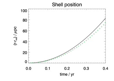
Figure 2: Radial position of the centre of mass of a 1D test cloud (green plus-symbols) over time compared to the analytic prediction (solid black line) for an optically thick cloud.

The setup follows essentially the scenario of paper I: We assume a hot atmosphere in approximate hydrostatic equilibrium, where the pressure follows a power law $p(x)=p_{0}x^{-s}$ with $x=r/r_{\mathrm{cld}}$ and $s=2$. Here, $r_{\mathrm{cld}}$ denotes the radial position of the cloud (distance from the SMBH) and $p_{0}=GM_{\mathrm{BH}}\rho_{0}(1-\Gamma)/r_{\mathrm{cld}}s$ is what the inter-cloud thermal pressure would be at that location, with $\rho_{0}=10^{8}m_{\mathrm{p}}$ cm^-3 and the Eddington factor $\Gamma=0.1$ ($l$ in paper I). Here, we take radiation pressure due to Thomson scattering into account. $G$ is the gravitational constant and $M_{\mathrm{BH}}$ the black hole mass, which is generally assumed to be $10^{8}$ solar masses. The density is given by $\rho(r)=\rho_{0}x^{1-s}$. The magnetic field (compare below) in the inter-cloud medium is perpendicular to the computational domain and contributes initially about ten per cent to the total pressure, above hydrostatic equilibrium. Yet, because of the cooling the atmosphere still develops an inwards flow over the simulation time.

The pressure level might appear high, yielding an inter-cloud temperature of order $10^{9}$ K. This is however necessary since we would like to test here the effect of dynamically relevant magnetic fields primarily inside the clouds. In order to yield a smaller thermal inter-cloud pressure, and therefore a temperature of order the Compton temperature, which one might expect, one would have to assume a much stronger magnetic field also in the inter-cloud medium. We defer the investigation of this situation to future work.

According to paper I, force equilibrium is reached for the cloud, if the rotational velocity in Kepler units is given by:

$$V_{\mathrm{eq}}^{2}=1-\frac{3\Gamma}{2\sigma_{T}N}\,,$$ (14)

where $N=2R_{\mathrm{cld}}\rho_{\mathrm{cld}}/m_{\mathrm{p}}$ is a measure of the column density of the cloud. In paper I, we have found that for high column densities, the clouds should be in a minimum of the effective potential, and therefore remain stable at their radial position. For low column densities, the clouds should be either ejected, or be sent inwards on an excentric orbit. For our pressure profile, the critical rotation velocity is 75 per cent of the Kepler velocity. All our clouds are set up on the stable branch of the equilibrium curve (compare Table 2). We found experimentally that we require a rotational velocity of 102 per cent of the value given in Equation 14 to ensure initial force equilibrium. The difference is due to the small amount of Thomson scattering in the ambient medium on the way to the cloud, which reduces the amount of radiation that actually arrives at the cloud.

For runs R34, R36 and R47, we use an azimuthal magnetic field, only. The plasma $\beta=8\pi p/B^{2}$ is initially set to 10 outside the cloud. Inside the cloud, we set the temperature to the minimum one (1000 K), and adjust the azimuthal magnetic field to yield pressure balance. This results in a magnetic field about three times stronger than in the inter-cloud medium, and a $\beta=10^{-4}$. Run R35 uses a uniform field strength inside and outside the cloud again with $\beta=10$ in the inter-cloud medium. This cloud is therefore initially underpressured. Runs R60, R61, R62 and R63 have an additional poloidal field (in the cloud, only). We have again $\beta=10$ in the inter-cloud medium. Within the cloud, the azimuthal field declines with distance from the cloud centre as a Gaussian:

$$B_{\phi}=B_{\phi,\mathrm{ic}}(1+3\,\mathrm{exp}(-10R^{2}/R_{\mathrm{cld}}^{2}))\,,$$ (15)

where $B_{\phi,\mathrm{ic}}$ is the azimuthal inter-cloud field, and capital $R$ refers to the distance from the cloud centre. $R_{\mathrm{cld}}$ is the cloud radius. The poloidal field is set up as closed field loop in a given meridional plane. The 3D structure would be helical. We initialise the radial component by

$$B_{r}=\frac{\alpha r_{\mathrm{cld}}}{r\sin\theta}\frac{\partial}{\partial\theta}B_{\phi}\sin\theta\,.$$ (16)

We have tried different values for $\alpha$. The one we report here is $\alpha=2\times 10^{-5}$. For this case, the initial peak values of the toroidal and poloidal field components are 103 G and 15 G, respectively. The magnetic field strength is for all runs generally around 30 G (the larger initial field in the runs with helical magnetic field decays quickly to this value), to ensure magnetically dominated clouds, following the considerations in section 2.

All boundary conditions are set to zero gradient for all variables. We believe that the best test for our radiation pressure module is the approximate stability of the hydrostatic halo, mentioned above. We have also checked 1D-cloud acceleration without gravity (Figure 2). In this test, the cloud accelerates a bit more slowly than expected from simple radiative acceleration of an optically thick cloud. This is, because the cloud also has to work against the ram pressure of the ambient medium.

5 Results

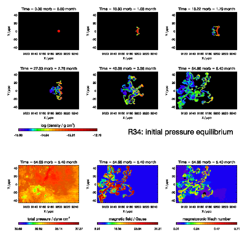
Figure 3: Evolution of run R34. The top six images show the logarithm of the density for different snapshot times, indicated in milli orbits (morb) and months on the individual images. The bottom three images show for the final snapshot from left to right: Total pressure, magnetic field strength and magnetosonic Mach number for the velocity component in the meridional plane. In the cold cloud gas, the magnetosonic speed is almost the same as the Alfvén speed.

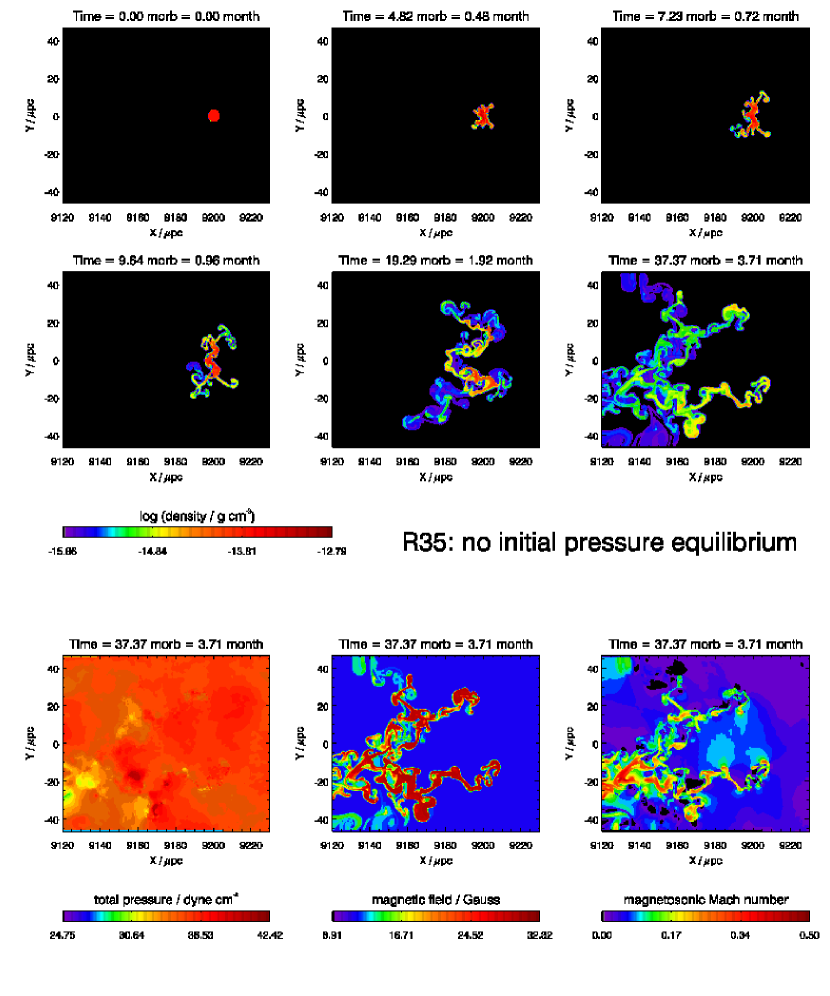
Figure 4: Same as Figure 3 for run R35.

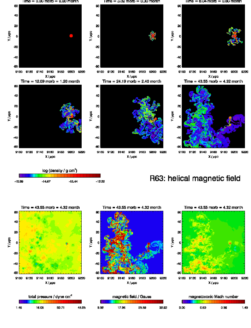
Figure 5: Same as Figure 3 for run R63. Only part of the computational domain is shown.

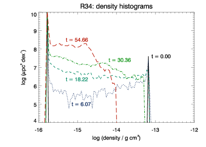
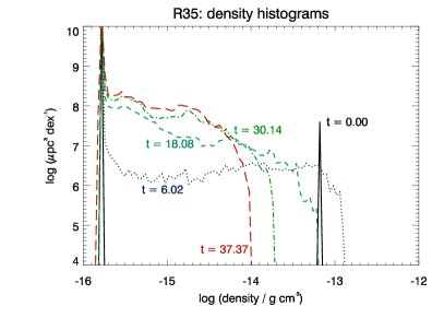
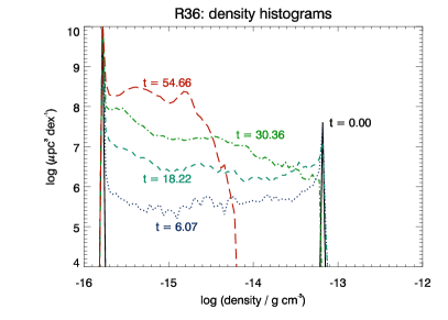
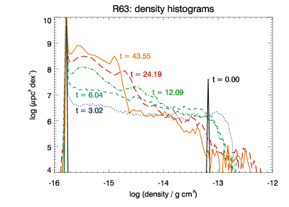
Figure 6: Density histograms for various runs, indicated in the individual titles and snapshot times (order: rder: solid black, dotted blue, dashed green, dot-dashed bright green, dashed red, solid orange), indicated in milli-orbits (morb) next to the respective lines. Mixing generally moves the upper density cutoff towards lower density (leftwards) for later times. The exception is run R63 for which the histogram converges at $t\approx 9$ morb and also continuously extends towards densities higher than the initial cloud density.

5.1 General dynamics

A general overview of the evolution of our simulated magnetised clouds is shown in Figures 3, 4 and  5. Movies are provided with the online version.

5.1.1 Pressure equilibrium

We first describe the evolution for run R34 (Figure 3), set up in initial total pressure equilibrium with an azimuthal magnetic field, only. The cloud is stationary at its radial position due to the matched radiative and centrifugal forces on the one hand, and the gravitational force on the other hand. This leads to a radial compression of the cloud (10.93 morb ($=$ milli-orbits)). At the same time, the magnetic pressure in the cloud increases. As there is no opposing force vertically, the cloud expands upwards and downwards, much like an open tube of toothpaste squeezed in the middle. This evolution matches the picture that Mathews (1982) described as the formation of quasar pancakes. Towards the edges of the cloud, the column density is lower, and therefore, there is a net outward force. This can be clearly identified in the 10.93 morb density plot. However, on the very edge, there is a certain amount of mixing. This will always happen to some extent, as the contact surface generally has to be resolved by a few grid cells. Wherever the cloud gas mixes with the ambient gas, the cloud looses rotational support and falls inwards. There is also some drag due to the inflow of the cooling ambient gas. A Rayleigh-Taylor instability due to the initial cloud acceleration is clearly seen in the middle of the cloud. The cloud continues to expand vertically by the tube of toothpaste mechanism, with lower column density regions being pushed outwards and mixing regions coming back inwards. By 40.08 morb, the cloud has dispersed into three major fragments with lower density (mixed) filaments falling inwards. The Kelvin-Helmholtz-timescale (Chandrasekhar 1961) is comparable to the evolution time:

$$\tau_{\mathrm{KH}}=1\,\mathrm{month}\frac{\lambda}{\mu\mathrm{pc}}\left(\frac{\eta}{0.005}\right)^{-1/2}\left(\frac{v}{200\,\mathrm{km}\,\mathrm{s}^{-1}}\right)^{-1}\,,$$ (17)

where $\lambda$ is the wavelength, $\eta$ the density ratio and $v$ the shear velocity. As expected, some filaments show the typical rolls of the Kelvin-Helmholtz instability. In the final snapshot (54.66 morb), all of the cloud material has mixed with the ambient gas to some degree, and falls leftwards, towards the SMBH. Mixing is a resolution effect in our simulations, but would also happen in reality at scales below our resolution. The mixing is further illustrated in the density histograms, which we show for similar snapshot times in Figure 6: Between $t=30.36$ morb and the final snapshot $t=54.66$ morb, the upper density cutoff drops by about a factor of five, indicating that the last cloudlet cores have been destroyed by mixing. Consequently, at this time, we also observe the cloud complex to start falling inwards as a whole. During the whole evolution time the entire simulated region stays well in pressure equilibrium (Figure 3, bottom left), the typical deviation being within ten per cent. Also, the magnetic field in the cloud complex remains close to its initial value of 31 Gauss (Figure 3, bottom middle). Acceleration is mediated by the compression of the magnetic field. We expect therefore the velocities to be limited by the Alfvén speed, $c_{\mathrm{a}}=B/\sqrt{4\pi\rho}\approx 500$ km/s in the cloud and $\approx 6000$ km/s in the ambient gas. Indeed, the observed velocities in the filaments are typically around 30 per cent of the Alfvén speed (Figure 3, bottom right, we use the magnetosonic speed in the Figures to show that also in the inter-cloud gas, the velocities remain sub-magnetosonic).

5.1.2 Underpressured cloud

We check the dependency on the initial condition in run R35 (Figure 4): Here the field strength is not higher inside the cloud, but set to the same value as in the ambient medium at the corresponding radius. The latter is still kept at $\beta=10$. Also, everything else is as in run R34. Now, the cloud is first compressed isotropically due to the initial underpressure before the radial (with respect to the black hole) compression phase. It overshoots and oscillates in size a few times. The acceleration produces Rayleigh-Taylor-instabilities on the cloud surface ($t=4.82$ morb). Then the cloud gets compressed anisotropically in radial (with respect to the black hole) direction ($t=7.23$ morb), and suffers a similar filamentation process than run R34, above ($t=9.64$ and $t=19.29$ morb). This initial phase proceeds significantly faster than for R34. Between $t=19.29$ morb and $t=37.37$ morb, the remaining dense cloudlet cores are dispersed (compare Figure 6), and at $t=37.37$ morb, the cloud is infalling towards the SMBH. The cloud, and respectively its fragments, is quickly compressed to the equilibrium magnetic field of 31 Gauss, gets quite close to pressure equilibrium and acquires velocities of about 30 per cent of the magnetosonic speed (Figure 4, bottom plots). Thus, with the exception of the initial phase, the evolution is very similar to the one of run R34.

5.1.3 Cloud with helical field

A significantly different result is obtained for a cloud with a helical magnetic field (R63, Figure 5). The cloud is initially not in force equilibrium, and first oscillates in size a few times. Similar to run R35, this has caused some filaments by $t=3.02$ morb. These filaments spread and disperse in much the same way as for the other runs. However, in contrast to the other runs, the cloud core remains remarkably stable, and is not significantly compressed by the radiative, centrifugal and gravitational forces. This situation remains essentially unchanged until the end of the simulation ($t=43.55$ morb), which we generally take to be the latest time before a significant amount of cloud gas has left the grid. The final equilibrium is characterised by a total overpressure of a factor of 1.3 in the cloud core, balanced by the magnetic tension force (Figure 5, bottom left). In the outer filaments, the magnetic field is of a very similar magnitude to the other simulations. It is about ten per cent higher in the cloud core. The velocities are typically about 60 per cent of the magnetosonic speed, only slightly higher than in the previous simulations and still sub-magnetosonic. Also the density histograms (Figure 6) are distinctly different from the previous runs: Whereas the histograms for the runs without a poloidal field component did not converge with time, with the upper density cutoff moving to lower densities at the end of the simulation, the density histograms for run R63 stay essentially constant from at least $t=24$ morb up to the end of the simulation at $t=44$ morb, which corresponds to almost $1/2$ of the simulation time. The occupied volume is roughly given by

$$\frac{\mathrm{d}V}{\mathrm{d\,log}\,\rho}\propto\rho^{-1}\,,$$ (18)

and also extends to densities exceeding the initial cloud density by a factor of ten.

Close-ups of the cloud core at the beginning and at the end of the simulation are shown in Figure 7. The cloud has essentially the same size as in the beginning. The density is however no longer homogeneous, but displays a round filamentary pattern, following the cloud surface. The magnetic field geometry is essentially identical to the one of the initial condition: a dominantly azimuthal core with a helix winding around. The peak value of the azimuthal field has however reduced by a factor of three, whereas the poloidal field strength remained almost unchanged.

Interestingly, many of the filaments that the cloud sheds are essentially devoid of poloidal field. Due to the solenoidal condition, filaments shed by the cloud need to have a bidirectional magnetic field. We have observed this at 0.1 G level near the cloud surface. But since they are often at the resolution limit, the poloidal field tends to cancel numerically, while the toroidal one is unaffected by this. Without poloidal field in the filaments, they disperse much like the filaments in the other simulations. Yet, sometimes filaments are shed which are thick enough to keep their poloidal field. Two such examples are present in Figure 7. Interestingly, they also adopt the field geometry of the parent cloud. This indicates that we may have found a magnetic field configuration for such clouds. It is clear that a poloidal field stabilises the cloud significantly.

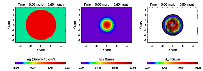
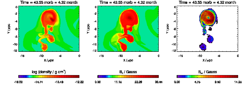
Figure 7: Close-up of the cloud core of run R63 at the beginning (top row) and at the end (bottom row) of the simulation. The logarithm of the density is shown on the left, the azimuthal magnetic field in the middle and the magnitude of the poloidal field with overlaid poloidal field vectors on the right. The coordinates are relative to the initial cloud centre. The slight upwards shift at the end of the simulation is due to an interaction with the boundary, which defines the end of the simulation.

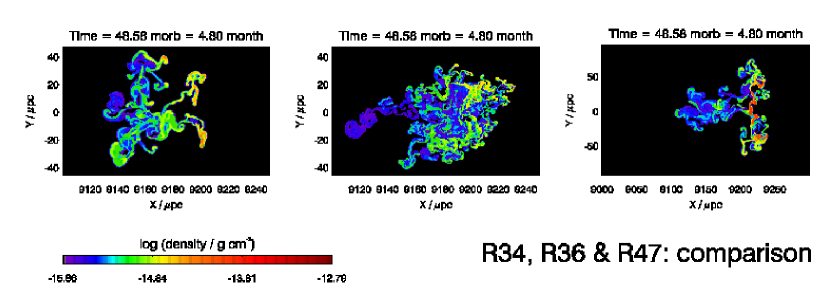
Figure 8: Comparison of the density distribution of run R34 (left) to run R36 (double resolution, middle) and run R47 (double spatial scales, right) at the common snapshot time of 4.58 morb.

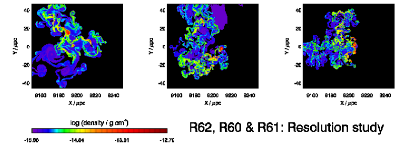
Figure 9: Comparison of the density distribution of run R60 (middle, smaller grid but otherwise identical to R63) to run R62 (half resolution, left) and run R61 (50 per cent higher resolution, right) at the common snapshot time of 48.58 morb.

5.2 Resolution dependence

We have re-simulated R34 at twice the spatial resolution (R36, Figure 8, middle). The evolution is quite similar to run R34, with the exception that the dispersion of the cloud and cloudlets happen faster. This may be seen from the more uniform appearance of the density distributions (Figure 8), but also from the density histograms (Figure 6), which are shown at the same timesteps: While the histograms at the corresponding times are generally very similar, the density cutoffs at $t=54.66$ morb differ by about 0.2 dex. Thus, the simulation can be regarded as overall numerically converged, but there is increased turbulent mixing at small scales for increasing resolution.

We have also studied the resolution dependence for run R63. For this study, we have used a smaller grid, because we have found that reflection of sound waves at the grid boundaries somewhat influences the motion of the filaments. R60 is the re-simulation of R63 at the same resolution. R62 uses 50 per cent less cells on a side, R61 has 50 per cent more cells on a side. Logarithmic density plots of all three runs at $t=48.58$ morb are shown in Figure 9. The filamentary systems are in general quite similar, though they have of course a finer structure at higher resolution. Yet, their extent and therefore kinematics is similar. The cloud core has drifted outward slightly for the two higher resolution runs. It is less dense and moving inwards for the low resolution run. The resolution is in this case not enough to resolve the cloud core structure, and therefore, the clouds disperses faster. This is also evident from the density histograms (Figure 10). The low resolution run lacks cloud material at high densities, which the two higher resolution clouds do show. It is interesting that this is in a way opposite to the case without poloidal field. There, higher resolution had made the cloud disperse quicker. Here, high resolution is essential to preserve the cloud core at high density. Our results are thus robust under resolution changes.

5.3 Scaling with cloud size

The simulations are not scalable, as the source terms introduce a dimensional scale to the problem. In order to explore the scaling behaviour, we re-simulated run R34 with all scales doubled (R47, Figure 8, right). As expected, the evolution now takes longer, but not nearly twice as long as for run R34. Otherwise, we find a very similar behaviour: Again the cloud is first compressed radially, then expands vertically by the tube of toothpaste mechanism, disperses into a filamentary system and then moves inwards due to the mixing related loss of rotational support and drag by the cooling infalling ambient gas.

5.4 Turbulent velocities

We define the mass-weighted root mean square poloidal velocity (rms velocity) by

$$v_{\mathrm{rms}}^{2} = \frac{\sum_{m}\mathrm{d}m\,({\bf v}_{\mathrm{p}}-\bar{\bf v}_{\mathrm{p}})^{2}}{\sum_{m}\mathrm{d}m}$$ (19)

$$\bar{\bf v}_{\mathrm{p}} = \frac{\sum_{m}\mathrm{d}m\,{\bf v}_{\mathrm{p}}}{\sum_{m}\mathrm{d}m}\,,$$ (20)

with the poloidal velocity vector ${\bf v}_{\mathrm{p}}$.

The dependency of $v_{\mathrm{rms}}$ on time is shown for all runs in Figure 11. The clouds set up in pressure equilibrium show first a shallow rise and then stay roughly constant. From the density histograms (Figure 6), the acceleration decreases when the densest cores are completely shredded. Hence, it seems that kinetic energy may be generated as long as dense cloud material may be squeezed radially and pushed out vertically. Since run R36 has a higher resolution than run R34, the gas may be compressed further. More energy is therefore stored temporarily in the magnetic field, which ultimately results in higher velocities. Run R47 has twice the spatial scales but is otherwise identical to run R34. The net force per unit volume has not changed. Since the initial densities are also the same, the accelerations in each cell are the same, too. Therefore, the turbulent velocities increase in a very similar way up to about 35 morb. Since the velocities are the same, but the length scale is twice as long in run R47, there is still room for more compression in simulation R47 at this time. Consequently, the turbulent velocity increases further, until the resolution limit is reached near 57 morb. One may understand the final turbulent velocity in terms of the total available space for compression: The gravitational and centrifugal forces act at similar strength in every cloud cell. The radiative force is concentrated on the illuminated surface. The net compression force is roughly $F=(1-V^{2})F_{\mathrm{G}}$, where $V$ is the initial rotation velocity of the cloud in Kepler units. The total energy transfered to the cloud in the limit of complete linear compression would therefore be:

$$E_{\mathrm{comp}}=\frac{1-V^{2}}{2}\pi F_{\mathrm{G}}R_{\mathrm{cld}}\,,$$ (21)

where the numerical factor is due to the average cloud thickness of $\pi R_{\mathrm{cld}}/2$. If this energy would be completely used for accelerating the cloud, a turbulent velocity of:

$$v_{\mathrm{t,c}} = \left(\pi(1-V^{2})R_{\mathrm{cld}}\frac{GM_{\mathrm{BH}}}{r_{\mathrm{cld}}^{2}}\right)^{1/2}$$

$$= 115\,\mathrm{km\,s}^{-1}\left(\frac{M_{\mathrm{BH}}}{10^{8}M_{\odot}}\right)^{1/2}\left(\frac{r_{\mathrm{cld}}}{9200\,\mu\mathrm{pc}}\right)^{-1}\left(\frac{R_{\mathrm{cld}}}{3\,\mu\mathrm{pc}}\right)^{1/2}$$

would result for $V=0.85$. As may be seen from Figure 11, the velocities are somewhat higher than this estimate. This is likely due to the increased radiative force during the lateral expansion of the clouds.

The clouds not set up in pressure equilibrium (R35 and R63) suffer initially a very quick increase of the rms velocity, as might have been expected. They evolve quickly towards pressure equilibrium. Then, as in the initial pressure equilibrium runs, the turbulent velocities change only gradually. Several curves show an upturn towards the end, which is due to the beginning interaction with the grid boundary.

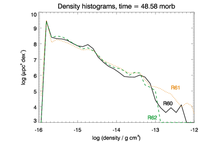
Figure 10: Density histograms for runs R60 (solid black) R61 (dotted yellow, 50 per cent higher resolution) and R62 (dashed green, half resolution) at 48.58 morb. The high density part disappears at low resolution.

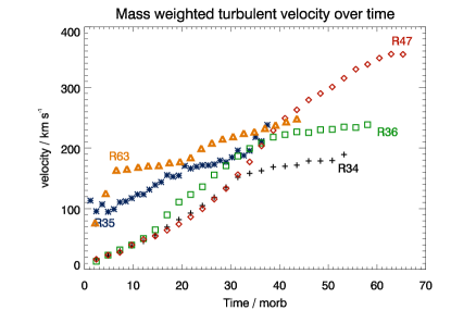
Figure 11: Mass-weighted root mean square velocities for runs R34 (black plus signs), R35 (blue stars), R36 (green squares), R47 (red diamonds) and R63 (orange triangles) over time. Only the poloidal velocity component is taken into account.

6 Discussion

We have investigated whether magnetic fields might contribute to the stability of BLR clouds. Stability is an issue in models without magnetic fields (compare section 1). We first combine literature data to get an idea of the magnitude of magnetic and other forces that might be relevant in this context. We find that reverberation mapping data is consistent with the bound cloud picture for a reasonable column density. Yet, the forces of radiation and gravity are comparable. We argue that the magnetic energy density, which sets the magnitude of the magnetic pressure and tension forces, should be at least of the same order of magnitude as the radiation pressure, in order to be at all able to contribute to the stability of the cloud. Estimating these parameters from the literature turned out to be complicated by the fact that the flux of radiation inferred via reverberation mapping studies leads to a rather high photoionisation parameter. One could take this as indication that there are no clouds at all and cloudless models like the one of Murray et al. (1995) should be preferred. Yet, for cloud densities on the high side of the allowed values, which would also mean that the typical BLRS would more likely be gravitationally bound, or when adopting other changes of the relevant parameters within the range allowed by the uncertainties, the photoionisation parameter may be brought down to a reasonable value.

A gravitationally bound cloud model entails the problem that the radiation leads to a surface force whereas gravity and centrifugal forces are body forces. Hence, an equilibrium configuration with these forces alone may not be found for the aforementioned assumptions. As all these forces act only radially away or towards the SMBH, an isotropic thermal pressure that was to stabilise the cloud against the compressive forces would necessarily also cause lateral expansion. Magnetic forces are anisotropic and are therefore in principal suited to counteract the compression and stabilise the clouds. We have performed MHD simulations with different magnetic field configurations to test this idea.

With an azimuthal magnetic field, only, the dynamics is dominated by the open tube of toothpaste mechanism: radial compression is followed by vertical expansion. Kelvin-Helmholtz and column density instabilities together with repeated, but smaller, tube of toothpaste squeezing events transform the initially homogeneous cloud quickly into a filamentary system. This result is in good agreement with the unstable pancake picture (Mathews 1982, 1986). In fact, in this case the effect of the magnetic field is just an additional pressure. Hence, the result remains essentially the same as in the pure hydrodynamic case. The cloud fragments are shredded down to the resolution level. Mixing with the pressure supported ambient gas reduces the rotational support, and the clouds fall inwards. Additionally, the atmosphere is not entirely stable and features some inwards flow due to the cooling. The timescale for this process is given first by the cloud compression timescale:

$$t_{\mathrm{c}} = \left(\frac{4R_{\mathrm{cld}}}{(1-V^{2})g/2}\right)^{1/2}$$

$$= 4\,\mathrm{months}\,\left(\frac{M_{\mathrm{BH}}}{10^{8}M_{\odot}}\right)^{-1/2}\left(\frac{r_{\mathrm{cld}}}{9200\,\mu\mathrm{pc}}\right)\left(\frac{R_{\mathrm{cld}}}{3\mu\mathrm{pc}}\right)^{1/2}\,,$$

where $g$ is the gravitational acceleration, and the evaluation is again for an initial rotation velocity $V=0.85$. Our numerical simulations show that clouds with an azimuthal magnetic field, only, are dispersed to the resolution level, and hence rapidly dissolve in the ambient medium within about $t_{\mathrm{c}}$, which is also similar to the Kelvin-Helmholtz timescale for the simulated cases. We show that the dispersal is even faster for higher resolution. The mixing, on the other hand, depends on the ambient density, via the Kelvin-Helmholtz timescale. It is therefore expected to be slower for lower ambient densities. Not much is known about the density in the inter-cloud gas. Assuming that the density would be lower by a factor of $10^{4}$, would increase the Kelvin Helmholtz timescale by a factor of 100, to the range of the orbital timescale. This would lead to extremely spread out pancake clouds, similar to the ones envisaged by Mathews (1986). We have also tried a factor of ten lower inter-cloud density than reported here. In this case, the cloud spreads quite quickly over the grid boundary probably due to the diminished resistance of the ambient gas, whereas the density histograms showed more dense gas at comparable times, as expected. In three dimensions, such pancake clouds would also face the ram pressure, which might also lead to compressed cloud heads with cometary tails, and a stability timescale of order the orbital timescale (Mathews 1986).

The runs with azimuthal magnetic field, only, underline the stability problem, and demonstrate clearly that our simulations are able to capture the destruction process adequately. Our runs with a helical magnetic field result in a much more stable cloud configuration, which survives the destruction process for the simulation time. The cloud corresponds to a helical filament in azimuthal direction. The core of this filament is dominated by the azimuthal field, producing an overpressure of about 30 per cent. This is balanced by the magnetic tension force of the poloidal field surrounding the core. The stability of the configuration results from the nature of the tension force which is inversely proportional to the curvature radius of the field lines. A radial compression straightens the field lines vertically (less radial tension force) and bends them more sharply at the vertical ends (increased vertical restoring tension force). A similar restoring force is obtained for compressions in every other direction. This configuration is very similar to the magnetic field used in tokamaks. One reason why it is employed in this context is precisely its MHD stability.

In order to isolate the effects of the magnetic field, we have used a negligible thermal cloud pressure. In our simulations we have realised this via a minimum temperature of 1000 K. The simulations would not have been any different had we used $10^{4}$ or even $10^{5}$ K, as the magnetic pressure would still be by far dominant in the clouds. We had initially decided for a low minimum temperature to check if the induced dynamics would lead to any significant increase of the cloud temperature via shock heating. The balance between shock heating and radiative cooling was found by Krause & Alexander (2007) in their simulations of clouds in jet cocoons to produce a peak in the temperature histograms around $10^{4}$ K. We do not find this effect here: Even for the late phases of R34, where the cloud is already essentially dispersed, the by far major part of the filaments remain close to the minimum temperature. Therefore, we do not find a heating mechanism which could compete with photoionisation.

Cloud stability in the limit of negligible magnetic fields has been studied extensively in the past (compare section 1). We have studied here the case of a dominant magnetic field compared to the thermal energy density, and separated the effects of magnetic pressure and magnetic tension. The azimuthal field behaves like a pressure in our axisymmetric simulations. Hence, we expect that we could in principle easily accommodate for a thermal pressure comparable to the magnetic one by replacing some or all of the magnetic pressure due to the azimuthal field by a corresponding thermal pressure. Details would of course depend on the effective equation of state, as the thermal pressure is affected by heating and cooling processes.

Another question one has to ask is how likely it would be to find such a helical configuration around real AGN. If the inter-cloud density would be comparable to the one assumed in our simulations, all unstable configurations would be shredded and dissolved within months. It is then quite difficult to replace the clouds quickly enough. If they would for example be launched from the accretion disc by a wind with velocities comparable to ones observed in the BLR, it would take a similar amount of time to be lifted to a significant altitude above the disc. Yet, the BLR cannot be a thin disc (e.g. Osterbrock 1978). Our helical field simulation has started quite far away from the final equilibrium, yet it has reached a stable configuration. It seems therefore possible that many different kinds of initial conditions eventually find an equilibrium solution. It is beyond the scope of this study how many stable filaments may be produced in given conditions of the interstellar medium.

Regarding the absolute magnitude of the magnetic field, Rees (1987) has already pointed out that magnetic field values of a few Gauss, as required here, are expected in BLRs due to relativistic winds, accretion flows or accretion driven winds. He also mentions the possibility of magnetic fields within the clouds if they are created by the thermal instability. We note that a similar value for the magnetic field has recently been estimated from their possible effects on the polarisation of the H$\alpha$ line (Silant’ev et al. 2012).

What level of internal turbulence do our simulations predict? We have argued that the available energy for turbulent motions is limited by the cloud compression and the Alfvén speed. Since the initial cloud volumes are unknown, we cannot make a quantitative prediction from this argument. If the BLR cloud population would be dominated by unstable clouds, being constantly shredded and replaced, we would predict turbulent velocities of about a third of the magnetosonic speed. If the radiation pressure would indeed be matched by the magnetic pressure in the cloud, the magnetosonic speed would be of order 1000 km/s, and the predicted internal velocities consequently a few hundred. For stable clouds of the helical type as shown above, we would expect even less in the cloud cores. Hence, the turbulent velocities of about 1000 km/s derived by Kollatschny & Zetzl (2011) cannot be reached in this way.

The cometary clouds observed by Maiolino et al. (2010), with dense cores and filamentary tails are compatible with our simulation results. Taking the orbital motion into account, the filamentary tails would be dominantly elongated in the azimuthal direction, as probably also in the observations. If these clouds would indeed be destroyed within a few months, as estimated by Maiolino et al. (2010), this would fit exactly with the destruction timescale of the radiative destruction mechanism discussed here.

In the literature one may find also BLR models that involve no clouds at all, e.g. the disc wind model of Murray et al. (1995). Here, the BLR forms the base of a wind accelerated by radiative and thermal pressure. The advantages and disadvantages of models with and without clouds have been nicely summarised by Netzer (2008): Cloud models provide a significantly better match to the emission line structures, while cloudless models obviously avoid the confinement problem altogether.

We have addressed the meridional stability problem, only. While this is certainly one of the major issues in the BLR cloud stability problem, we have not shown that the cloud would also survive 3D effects. From the MHD point of view, kink instabilities are likely to occur, which would cause bends in the cloud filament along its major axis. Further, the clouds are unlikely to be extended along the entire azimuthal angle as necessarily implied in our axisymmetric simulations. In reality, the clouds could still be elongated substantially in the azimuthal direction, if the ends would be anchored in a thinner disc structure, similar to coronal loops on the surface of the sun. In simple magnetic field configurations with closed field lines within the cloud, the field could of course be transformed via reconnection, which would likely lead to cloud splitting as each closed field region could support a cloud on its own. An azimuthally extended cloud with the azimuthal field closing at the ends and returning through some part of the cloud would be expected to expand in the polar direction and form something like a closed ring. For any non-axisymmetric clouds, also the ram pressure would be significant. For our cloud setups the azimuthal ram pressure would be comparable to the magnetic pressure in the cloud. If one can find magnetic field configurations that would also stabilise against this effect is beyond the scope of the present investigation.

In order to reach pressure equilibrium with the clouds, also the inter-cloud medium should be magnetised on a similar level. This might be accessible to Faraday rotation. The expected rotation measure would be of order

$$\mathrm{RM}=8.12\times 10^{8}\int_{0}^{L}n_{\mathrm{e,6}}{B}\cdot\mathrm{d}l\;\mathrm{rad\,m^{-2}},$$ (24)

where the path-length d$l$ is measured in units of $10^{-3}$ pc, $B$ in Gauss and the electron density in units of $10^{6}$ cm^-3. As mentioned above, the density is uncertain, and could also be a few orders of magnitude lower. For a turbulent medium, one would therefore predict that signals below $\approx 10^{13}$ Hz ($\lambda>30\mu$m) would be depolarised (Krause, Alexander, & Bolton 2007). This prediction might therefore be tested in the future by infrared polarimetry, if one is sure to observe emission from a jet base.

For our simulations, a change in the geometry of the magnetic field in the inter-cloud region should not matter much, because the thermal energy density dominates there over the magnetic one. As long as the forces are set up close to equilibrium, we would expect an outcome in between runs R34 (initial pressure equilibrium) and R35 (no initial pressure equilibrium). In reality, the situation might of course be more complex, and the inter-cloud medium might be magnetically dominated and at the same time have a non-zero poloidal component. It would then be important if the magnetic field would be topologically connected to the clouds. In that case, the cloud gas could escape along the field lines. It might also happen that regions of space with a favourable magnetic field configuration might protect new clouds which are just forming from the thermal instability. Yet, these complexities are beyond the scope of the present discussion.

Summarising, we find some indication that bound BLR clouds might indeed be stabilised by the magnetic field against collapse due to opposing radiative and gravitational forces. In this case, the magnetic field would have to have a poloidal component.

7 Conclusions

Gravitationally bound clouds facing strong radiation pressure are unstable in the purely hydrodynamic case because radiative and gravitational forces compress the clouds radially, whereas the thermal pressure acts isotropic. They may be more stable if they are significantly magnetised. In particular, we find in axisymmetric magnetohydrodynamic simulations with a prescription for the radiation pressure that the magnetic tension force produces more stable clouds, while in a situation where the geometry of the magnetic field is such that its effect is only analogous to an additional pressure, the clouds are similarly unstable as in the hydrodynamic case. In order to be effective, in the BLRs of a discussed sample of AGN, the magnetic field strength should be of order a few Gauss, accurate to about an order of magnitude and constrained by the condition that magnetic, radiative and gravitational forces should be comparable.

References

- Bentz et al. (2006) Bentz M. C. et al., 2006, ApJ, 651, 775
- Bentz et al. (2007) Bentz M. C. et al., 2007, ApJ, 662, 205
- Bentz et al. (2009) Bentz M. C. et al., 2009, ApJ, 705, 199
- Blumenthal & Mathews (1975) Blumenthal G. R., Mathews W. G., 1975, ApJ, 198, 517
- Blumenthal & Mathews (1979) —, 1979, ApJ, 233, 479
- Chandrasekhar (1961) Chandrasekhar S., 1961, Hydrodynamic and hydromagnetic stability, Clarendon, Oxford
- Denney et al. (2006) Denney K. D. et al., 2006, ApJ, 653, 152
- Denney et al. (2009) Denney K. D. et al., 2009, ApJ, 704, L80
- Dopita & Sutherland (2003) Dopita M. A., Sutherland R. S., 2003, Astrophysics of the diffuse universe. Springer (Berlin, New York), Astronomy and astrophysics library, ISBN 3540433627
- Ferland & Elitzur (1984) Ferland G. J., Elitzur M., 1984, ApJ, 285, L11
- Ferland et al. (1992) Ferland G. J., Peterson B. M., Horne K., Welsh W. F., Nahar S. N., 1992, ApJ, 387, 95
- Grier et al. (2008) Grier C. J. et al., 2008, ApJ, 688, 837
- Hopkins et al. (2007) Hopkins P. F., Richards G. T., Hernquist L., 2007, ApJ, 654, 731
- Kollatschny & Zetzl (2011) Kollatschny W., Zetzl M., 2011, Nature, 470, 366
- Krause & Alexander (2007) Krause M., Alexander P., 2007, MNRAS, 376, 465
- Krause et al. (2007) Krause M., Alexander P., Bolton R., 2007, in Proceedings of the Conference: ”From Planets to Dark Energy: the Modern Radio Universe”, Manchester 2007, Proceedings of Science, POS(MRU)109, http://pos.sissa.it
- Krause et al. (2011) Krause M., Burkert A., Schartmann M., 2011, MNRAS, 411, 550 (paper I)
- Krolik (1988) Krolik J. H., 1988, ApJ, 325, 148
- Krolik et al. (1981) Krolik J. H., McKee C. F., Tarter C. B., 1981, ApJ, 249, 422
- Kwan & Krolik (1981) Kwan J., Krolik J. H., 1981, ApJ, 250, 478
- Leighly & Casebeer (2007) Leighly K. M., Casebeer D., 2007, in Astronomical Society of the Pacific Conference Series, Vol. 373, The Central Engine of Active Galactic Nuclei, L. C. Ho & J.-W. Wang, ed., p. 365
- Maiolino et al. (2010) Maiolino R. et al., 2010, A&A, 517, A47
- Marconi et al. (2008) Marconi A., Axon D. J., Maiolino R., Nagao T., Pastorini G., Pietrini P., Robinson A., Torricelli G., 2008, ApJ, 678, 693
- Marconi et al. (2009) Marconi A., Axon D. J., Maiolino R., Nagao T., Pietrini P., Risaliti G., Robinson A., Torricelli G., 2009, ApJ, 698, L103
- Mathews (1976) Mathews W. G., 1976, ApJ, 207, 351
- Mathews (1982) —, 1982, ApJ, 252, 39
- Mathews (1986) —, 1986, ApJ, 305, 187
- Mathews & Doane (1990) Mathews W. G., Doane J. S., 1990, ApJ, 352, 423
- McKee & Tarter (1975) McKee C. F., Tarter C. B., 1975, ApJ, 202, 306
- Murray et al. (1995) Murray N., Chiang J., Grossman S. A., Voit G. M., 1995, ApJ, 451, 498
- Netzer (2008) Netzer H., 2008, New Astronomy Review, 52, 257
- Netzer (2009) —, 2009, ApJ, 695, 793
- Netzer & Marziani (2010) Netzer H., Marziani P., 2010, ApJ, 724, 318
- Onken et al. (2004) Onken C. A., Ferrarese L., Merritt D., Peterson B. M., Pogge R. W., Vestergaard M., Wandel A., 2004, ApJ, 615, 645
- Osterbrock (1978) Osterbrock D. E., 1978, Proceedings of the National Academy of Science, 75, 540
- Osterbrock (1988) —, 1988, Astrophysics of gaseous nebulae and active galactic nuclei. University Science Books, Sausalito, CA
- Osterbrock & Mathews (1986) Osterbrock D. E., Mathews W. G., 1986, ARA&A, 24, 171
- Peterson (1988) Peterson B. M., 1988, PASP, 100, 18
- Peterson (1997) —, 1997, active galactic nuclei. Cambridge University Press
- Peterson et al. (2004) Peterson B. M. et al., 2004, ApJ, 613, 682
- Rees (1987) Rees M. J., 1987, MNRAS, 228, 47P
- Rees et al. (1989) Rees M. J., Netzer H., Ferland G. J., 1989, ApJ, 347, 640
- Risaliti et al. (2011) Risaliti G., Nardini E., Salvati M., Elvis M., Fabbiano G., Maiolino R., Pietrini P., Torricelli-Ciamponi G., 2011, MNRAS, 410, 1027
- Schartmann et al. (2011) Schartmann M., Krause M., Burkert A., 2011, MNRAS, 415, 741
- Silant’ev et al. (2012) Silant’ev N. A., Gnedin Y. N., Buliga S. D., Piotrovich M. Y., Natsvlishvili T. M., 2012, ArXiv astro-ph 1203.2763
- Smith et al. (2005) Smith J. E., Robinson A., Young S., Axon D. J., Corbett E. A., 2005, MNRAS, 359, 846
- Snedden & Gaskell (2007) Snedden S. A., Gaskell C. M., 2007, ApJ, 669, 126
- Sun & Malkan (1989) Sun W.-H., Malkan M. A., 1989, ApJ, 346, 68
- Sutherland & Dopita (1993) Sutherland R. S., Dopita M. A., 1993, ApJS, 88, 253
- Tarter & McKee (1973) Tarter C. B., McKee C. F., 1973, ApJ, 186, L63
- van Leer (1977) van Leer B., 1977, Journal of Computational Physics, 23, 276
- Ziegler & Yorke (1997) Ziegler U., Yorke H. W., 1997, Computer Physics Communications, 101, 54