Test MaxEnt in Social Strategy Transitions with Experimental Two-Person Constant Sum 2$\times$2 Games

Abstract

Abstract

Using laboratory experimental data, we test the uncertainty of social state transitions in various competing environments of fixed paired two-person constant sum $2\times 2$ games. It firstly shows that, the distributions of social strategy transitions are not erratic but obey the principle of the maximum entropy (MaxEnt). This finding indicates that human subject social systems and natural systems could share wider common backgrounds.

I Introduction

The principle of the maximum entropy (MaxEnt) is introduced by Jaynes Jaynes1957 , rooting in Boltzmann, Gibbs and Shannon Shannon1948 ; Jaynes2003 . As a methodology, MaxEnt has gained its wide applications in natural science and engineering. The advantage of this methodology is to provide rich information based on very limit information. In economics, MaxEnt approach has also gained its wide applications, e.g., in market equilibrium Toda2010 ; Barde2012 , in wealth and income distribution Castaldi2007 ; WuMaxEntIncome2003 , in firm growth rates Alfarano2008 and in behavior modeling Wolpert2012 . Theoretical interpreting or modeling of the distributions of social outcomes with MaxEnt is growing.

Considering the importance of MaxEnt, to carry out laboratory experiments to investigate this fundamental rule is necessary Falk2009 . Only quite recently, entropy is firstly measured in experimental economics systems to evaluate social outcomes by Bednar et.al. Yan2011 and Cason et.al cason2011behavioral . Then, Xu et.al., XuetalMaxEnt2012 find the human system in laboratory fixed-paired two-person constant-sum 2 $\times$ 2 games obey the MaxEnt. To the best of our knowledge, these are almost the total experimental works related to entropy or MaxEnt in social research field till now. In the first experimental investigation in MaxEnt, Xu et.al. XuetalMaxEnt2012 focus on the static observable — distribution and the entropy. A direct one-step-forward question is, in the experimental social interaction systems, whether the dynamic observable fits MaxEnt or not?

Answering this question is the main aim of this report. The paper is organized as follow: section two describes the relative notions; section three introduces the experiments and reports the experimental social transitions; section four provides the MaxEnt prediction relating to the social transitions of the investigated experiments; section five reports the results; Discussion and summary are at last.

II Relative Notions

II.1 Two person constant sum $2\times 2$ game

Two-person zero-sum games describe situations in which two individuals are absolutely opposite to each other, where one’s gain is always the other’s loss myerson1997game . Constant sum game is strategically equivalent to zero sum games in mathematical view.

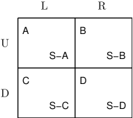
Figure 1: Payoff Matrix of a Constant Sum Game. A, B, C and D are the payoffs for row player under four combinations of two player’s strategies respectively and S-A, S-B, S-C and S-D are for column player respectively. S denotes the sum of the payoffs to the two players.

In a two-person constant-sum game, each player has two strategies. For a row player, the strategy set is $(U,D)$ and for a column player, the strategy set is $(L,R)$. The sum of the two players’ payoffs is the same for any outcome. Let S denote the sum of the payoffs of the two players. Any constant sum 2 $\times$ 2 game can be written in the form of Fig. 1. A, B, C and D is the payoff for row player under four combinations of two players’ strategies respectively and S-A, S-B, S-C and S-D are for column player respectively. If $(A>C)\cap(B<D)\cap(A>B)\cap(C<D)$ or $(A<C)\cap(B>D)\cap(A<B)\cap(C>D)$ as in selten2008 , there exists an unique mixed strategy Nash equilibrium (MSNE).

II.2 Social State and Observation

The social state $x_{ij}$ Sandholm2009Encyclopedia can be taken as the combination of two players’ strategies, herein $i$ indicates the column player’s strategy and $j$ indicates the row player’s strategy. Let $p$ be the probability of strategy R for column player and $q$ be the probability of strategy D for row player, the social state can be described by $x_{ij}$=$(p,q)$. During a game, each player chooses a pure strategy from his own strategy set in a round $t$, the combination of these two strategies can be taken as a social state $x_{t}$ in that round, $x_{t}$ = $(p_{t},q_{t})$. Obviously, there are altogether four possible social states in one round, i.e., (0,0), (0,1), (1,0) and (1,1) indicating LU, LD, RU and RD respectively, and we simplify them as $x_{00}$, $x_{01}$, $x_{10}$, and $x_{11}$. In Fig. 2(b) and (f), the gray dots present the social states.

If the game is repeated, observation denoted as $\Omega_{ij}$ at each state $x_{ij}$ can be accumulated and the results of these games are shown in the last 4 columns of Tab 1.

II.3 Social transition

In this paper, we investigate the social transitions within the strategy states in the strategy space. In a repeated game, for a given round $t$, the social state is $x_{t}=(p_{t},q_{t})$; similarly, the social state in the previous round can be denoted as $x_{t-1}:=(p_{t-1},q_{t-1})$ and in the next round can be denoted as $x_{t+1}:=(p_{t+1},q_{t+1})$. For each given round $t$, there exists the next round and previous round except the first round and last round in a experimental session. So, there exists a social forward transition vector (denoted as $T_{+}$) indicating the transition from $x_{t}$ to $x_{t+1}$, and a social backward transition vector (denoted as $T_{-}$) indicating the transition from $x_{t-1}$ to $x_{t}$.

In a two-person 2$\times$2 game, there are four social states, so there are all 32 transitions (shown in the first column in Table 2), including the 4 backward (forward) transitions for each of the 4 states. These 32 transitions should be the samples for MaxEnt testing.

II.4 Distribution of Transitions of a Given State

During a game, for a given social state, there exists 4 forward transitions and 4 backward transitions, respectively. This means that there should exist a distribution of transitions.

For example, Fig. 2 (a) is demonstrating the distribution of the transitions of the given state $x_{01}$, in which the four backward transitions $T_{01{\leftarrow}00}$, $T_{01{\leftarrow}01}$,$T_{01{\leftarrow}10}$ and $T_{01{\leftarrow}11}$ come from the four state $x_{00}$, $x_{01}$, $x_{10}$ and $x_{11}$, respectively; the blue arrows indicate the directions of transitions and the numerics indicate the related actual frequencies. The distribution of backward transitions $T_{01{\leftarrow}00}$, $T_{01{\leftarrow}01}$,$T_{01{\leftarrow}10}$, $T_{01{\leftarrow}11}$ are 55, 106, 78, and 193, respectively. Similarly, Fig. 2 (e) illustrates the distribution of the forward transitions.

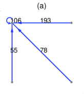
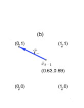
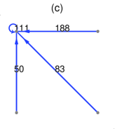
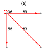
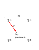
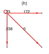
Figure 2: Transition distribution and aggregated transition. (a) four actual backward transitions $T_{01{\leftarrow}00}$, $T_{01{\leftarrow}01}$,$T_{01{\leftarrow}10}$, $T_{01{\leftarrow}11}$ for the given state $x_{01}$ from $x_{00}$, $x_{01}$, $x_{10}$, $x_{11}$; the blue arrows indicate the directions of transitions; the numerics indicate the frequencies of transitions, respectively; (b) the aggregated backward transition $\bar{T}_{-}$ and related mean starting point ${\bar{x}_{t-1}}$ = ${(\bar{p}_{t-1},\bar{q}_{t-1})}$ = $(0.63,0.69)$; (c) four expected backward transitions for $x_{01}$ from four starting points $x_{00}$, $x_{01}$, $x_{10}$, $x_{11}$ with MaxEnt, the blue arrows indicate the directions of transitions and the numerics indicate the related frequencies; (d) an example which is not in agreement with MaxEnt but satisfies the aggregated backward transition constraint in (b);(e) four actual forward transitions $T_{01{\rightarrow}00}$, $T_{01{\rightarrow}01}$, $T_{01{\rightarrow}10}$, $T_{01{\rightarrow}11}$ from $x_{01}$, the red arrows indicate the directions of transitions, and the numerics indicate the related actual frequencies of transitions; (f) the aggregated forward transition $\bar{T}_{+}$ and relative mean terminal point ${\bar{x}_{t+1}}$ = $({\bar{p}_{t+1}},{\bar{q}_{t+1}})$ = $(0.40,0.45)$; (g) four MaxEnt expected forward transitions; (h) an example which is not in agreement with MaxEnt but satisfies the actual aggregated forward transition constraint. Data in (a) and (e) comes from the experiment — game 1.

II.5 Aggregated Transition of a State

The existence of distribution of transitions of a given state implicates that there are many backward starting points and forward terminal points. So, for a given state $x_{i_{0}j_{0}}$, we can get a so-called the mean starting point ${\bar{x}_{t-1}}$=${(\bar{p}_{t-1},\bar{q}_{t-1})}$ and a aggregated backward transition $\bar{T}_{-}$ (it is natural that $\bar{T}_{-}$=${x_{i_{0}j_{0}}-\bar{x}_{t-1}}$), and also the mean terminal point ${\bar{x}_{t+1}}$ = $({\bar{p}_{t+1}},{\bar{q}_{t+1}})$ and a aggregated forward transition $\bar{T}_{+}$ (it is natural that $\bar{T}_{+}$=${\bar{x}_{t+1}}-x_{i_{0}j_{0}}$). The aggregated forward transition $T_{+}$ is the same as the experimental dynamics observable in literatures (called as change in a given state in ref. HuyckSamuelson2001 and the mean jump-out vector of a given state in ref XuWang2011ICCS ).

For example, supposing the given state is (0,1), Fig. 2 (b) illustrates the aggregated backward transition $\bar{T}_{-}$, as the average of the four vectors in Fig. 2 (a), is (-0.63,0.31); Meanwhile the mean starting point ${\bar{x}_{t-1}}$=$(0.63,0.69)$; In Fig. 2 (f), $\bar{T}_{+}$, as the average of the four vectors in Fig. 2 (e), is (0.40,-0.55) and then ${\bar{x}_{t+1}}$=$(0.40,0.45)$.

III Data Set and Experimental Transitions

III.1 Experiments and Data set

Experimental economics methods are well suited to evaluate theories Falk2009 . In this paper, we use the same data set as ref XuetalMaxEnt2012 to test the MaxEnt in social strategy transitions. The two-person constant sum 2$\times$2 game includes 11 different parameters (Table 1). From game 1 to game 10, each game consists of 9 pairs of subjects, each pair play for 500 rounds while for game 11, the game consists of 12 pairs of subjects, each pair play for 300 rounds. These yield 4500 observed social states in each of game 1 to game 10 and 3600 observed social states in game 11 (for more detail, see ref. RothErev2007 ; XuetalMaxEnt2012 ).

Table 1: Parameters and observations of the 11 game^§

game	A	B	C	D	S	Group	Rounds	$\Omega_{00}$	$\Omega_{01}$	$\Omega_{10}$	$\Omega_{11}$
g1	77	35	8	48	100	9	500	994	433	1659	1405
g2	73	74	87	20	100	9	500	1373	250	2401	467
g3	63	8	1	17	100	9	500	664	333	1955	1539
g4	55	75	73	60	100	9	500	643	1611	588	1649
g5	5	64	93	40	100	9	500	548	891	1153	1899
g6	46	54	61	23	100	9	500	1135	706	1729	921
g7	89	53	82	92	100	9	500	502	1840	825	1324
g8	88	38	40	55	100	9	500	353	663	1443	2032
g9	40	76	91	23	100	9	500	1157	860	1366	1108
g10	69	5	13	33	100	9	500	443	465	995	2588
g11	5	0	0	5	5	12	300	837	913	907	931

• g1 to g11 indicate game 1 to game 11, respectively. The symbols A, B, C, D and S refer to Fig. 1. Group is the number of the pairs of human subjects playing the games. Rounds is the game repeated times in each pair.

III.2 Experimental Distributions of Transitions

According to the data set for each of the 11 games, using the definition in Sec. II.3 and II.4, we can calculate the actual experimental distributions of backward transitions and forward transitions. The results are summarized in Table 2, which should serve as the targets for testing MaxEnt.

III.3 Experimental Aggregated Transition for Each State

Numerically, $\bar{x}_{t\pm 1}$ can be presented by two components ($\bar{p}_{t\pm 1},\bar{q}_{t\pm 1}$). Using the definition in Sec. II.5, results of all of the components from experiments are shown in Table 3. The vectors, $\bar{x}_{t\pm 1}$, are shown in the sub-figures in Fig. 3.

For calculating the theoretical backward (forward) distributions of the transitions from MaxEnt, $\bar{x}_{t-1}$ ($\bar{x}_{t+1}$) should constraint the testing of MaxEnt.

Table 2: Actual frequencies of the transitions of 11 games

$T_{-}$	g1	g2	g3	g4	g5	g6	g7	g8	g9	g10	g11
$T_{00{\leftarrow}00}$	464	764	184	314	124	529	143	111	606	116	196
$T_{00{\leftarrow}01}$	155	52	73	67	68	99	169	95	67	139	241
$T_{00{\leftarrow}10}$	274	504	327	193	207	382	89	70	362	123	182
$T_{00{\leftarrow}11}$	102	53	79	66	149	124	98	75	120	63	218
$T_{01{\leftarrow}00}$	55	86	35	239	213	226	104	11	263	43	149
$T_{01{\leftarrow}01}$	106	48	89	1054	217	311	1191	264	365	121	216
$T_{01{\leftarrow}10}$	78	69	100	70	191	86	66	62	85	55	231
$T_{01{\leftarrow}11}$	193	45	111	245	268	85	482	327	145	247	319
$T_{10{\leftarrow}00}$	401	446	383	45	51	235	145	169	144	232	281
$T_{10{\leftarrow}01}$	83	75	99	65	143	86	99	82	99	91	263
$T_{10{\leftarrow}10}$	1021	1722	1046	258	483	1029	478	858	691	370	191
$T_{10{\leftarrow}11}$	152	160	424	223	476	380	103	333	434	302	173
$T_{11{\leftarrow}00}$	74	77	62	45	160	145	110	62	144	52	211
$T_{11{\leftarrow}01}$	89	75	72	425	463	210	381	222	329	114	193
$T_{11{\leftarrow}10}$	286	106	482	67	272	232	192	453	228	447	303
$T_{11{\leftarrow}11}$	958	209	925	1115	1006	332	641	1297	409	1976	221
$T_{+}$	g1	g2	g3	g4	g5	g6	g7	g8	g9	g10	g11
$T_{00{\rightarrow}00}$	464	764	184	314	124	529	143	111	606	116	196
$T_{00{\rightarrow}01}$	55	86	35	239	213	226	104	11	263	43	149
$T_{00{\rightarrow}10}$	401	446	383	45	51	235	145	169	144	232	281
$T_{00{\rightarrow}11}$	74	77	62	45	160	145	110	62	144	52	211
$T_{01{\rightarrow}00}$	155	52	73	67	68	99	169	95	67	139	241
$T_{01{\rightarrow}01}$	106	48	89	1054	217	311	1191	264	365	121	216
$T_{01{\rightarrow}10}$	83	75	99	65	143	86	99	82	99	91	263
$T_{01{\rightarrow}11}$	89	75	72	425	463	210	381	222	329	114	193
$T_{10{\rightarrow}00}$	274	504	327	193	207	382	89	70	362	123	182
$T_{10{\rightarrow}01}$	78	69	100	70	191	86	66	62	85	55	231
$T_{10{\rightarrow}10}$	1021	1722	1046	258	483	1029	478	858	691	370	191
$T_{10{\rightarrow}11}$	286	106	482	67	272	232	192	453	228	447	303
$T_{11{\rightarrow}00}$	102	53	79	66	149	124	98	75	120	63	218
$T_{11{\rightarrow}01}$	193	45	111	245	268	85	482	327	145	247	319
$T_{11{\rightarrow}10}$	152	160	424	223	476	380	103	333	434	302	173
$T_{11{\rightarrow}11}$	958	209	925	1115	1006	332	641	1297	409	1976	221

• g1 indicates game 1, the rest analogize.

IV Theoretical Distributions of Transitions from MaxEnt

In this paper, in order to have a deeper insight in the dynamic social observable, we use the aggregated social transitions ($T_{\pm}$) as the constraints for MaxEnt testing. It is clear that for a given state, without MaxEnt, the distribution of backward (forward) transitions can be arbitrary even given the constraints $T_{\pm}$ (two examples are given in discussion).

Table 3: Mean starting point $\bar{x}_{t-1}$ and terminal point $\bar{x}_{t+1}$

state	${\bar{x}_{t-1}}$	g1	g2	g3	g4	g5	g6	g7	g8	g9	g10	g11
$x_{00}$	${\bar{p}_{t-1}}$	0.38	0.41	0.61	0.40	0.65	0.45	0.37	0.41	0.42	0.42	0.48
	${\bar{q}_{t-1}}$	0.26	0.08	0.23	0.21	0.40	0.20	0.54	0.48	0.16	0.46	0.55
$x_{01}$	${\bar{p}_{t-1}}$	0.63	0.46	0.63	0.20	0.52	0.24	0.30	0.59	0.27	0.65	0.60
	${\bar{q}_{t-1}}$	0.69	0.38	0.6	0.81	0.55	0.56	0.91	0.89	0.59	0.79	0.58
$x_{10}$	${\bar{p}_{t-1}}$	0.71	0.78	0.75	0.81	0.83	0.81	0.70	0.83	0.82	0.68	0.40
	${\bar{q}_{t-1}}$	0.14	0.10	0.27	0.49	0.54	0.27	0.24	0.29	0.39	0.39	0.48
$x_{11}$	${\bar{p}_{t-1}}$	0.88	0.67	0.91	0.72	0.67	0.61	0.63	0.86	0.57	0.94	0.56
	${\bar{q}_{t-1}}$	0.74	0.61	0.65	0.93	0.77	0.59	0.77	0.75	0.66	0.81	0.45
state	${\bar{x}_{t+1}}$	g1	g2	g3	g4	g5	g6	g7	g8	g9	g10	g11
$x_{00}$	${\bar{p}_{t+1}}$	0.48	0.38	0.67	0.14	0.39	0.33	0.51	0.65	0.25	0.64	0.59
	${\bar{q}_{t+1}}$	0.13	0.12	0.15	0.44	0.68	0.33	0.43	0.21	0.35	0.21	0.43
$x_{01}$	${\bar{p}_{t+1}}$	0.40	0.60	0.51	0.30	0.68	0.42	0.26	0.46	0.50	0.44	0.50
	${\bar{q}_{t+1}}$	0.45	0.49	0.48	0.92	0.76	0.74	0.85	0.73	0.81	0.51	0.45
$x_{10}$	${\bar{p}_{t+1}}$	0.79	0.76	0.78	0.55	0.65	0.73	0.81	0.91	0.67	0.82	0.54
	${\bar{q}_{t+1}}$	0.22	0.07	0.30	0.23	0.40	0.18	0.31	0.36	0.23	0.5	0.59
$x_{11}$	${\bar{p}_{t+1}}$	0.79	0.79	0.88	0.81	0.78	0.77	0.56	0.80	0.76	0.88	0.42
	${\bar{q}_{t+1}}$	0.82	0.54	0.67	0.82	0.67	0.45	0.85	0.80	0.50	0.86	0.58

• g1 indicates game 1, the rest analogize.

For a given state $x_{i_{0}j_{0}}$, the $\bar{x}_{t-1}$ is assumed to be $(\bar{p}_{t-1},\bar{q}_{t-1})$ and there is no other information. According to MaxEnt suggested by Jaynes Jaynes2003 , the probability of the backward transitions from the states to $x_{i_{0}j_{0}}$ can be expressed, respectively, as

$$p(T_{i_{0}j_{0}\leftarrow 00}|\bar{x}_{t-1}) = (1-\bar{p}_{t-1})^{1-i}(1-\bar{q}_{t-1})^{1-j}$$

$$p(T_{i_{0}j_{0}\leftarrow 01}|\bar{x}_{t-1}) = \bar{q}_{t-1}^{j}(1-\bar{p}_{t-1})^{1-i}$$

$$p(T_{i_{0}j_{0}\leftarrow 10}|\bar{x}_{t-1}) = \bar{p}_{t-1}^{i}(1-\bar{q}_{t-1})^{1-j}$$

$$p(T_{i_{0}j_{0}\leftarrow 11}|\bar{x}_{t-1}) = \bar{p}_{t-1}^{i}\bar{q}_{t-1}^{j}$$

More compactly, the probability of backward transitions from $x_{ij}$ to $x_{i_{0}j_{0}}$, can be expressed as,

$$p(T_{i_{0}j_{0}\leftarrow ij}|\bar{x}_{t-1})=\bar{p}_{t-1}^{i}(1-\bar{p}_{t-1})^{1-i}\bar{q}_{t-1}^{j}(1-\bar{q}_{t-1})^{1-j},$$ (1)

in which $\{i,j\}\in\{0,1\}$. Similarly, for $\bar{x}_{i_{0}j_{0}}$ and its $\bar{x}_{t+1}$=($\bar{p}_{t+1},\bar{q}_{t+1}$), the probability of the forward transition from $x_{i_{0}j_{0}}$ to state $x_{ij}$ can be expressed as

$$p(T_{i_{0}j_{0}\rightarrow ij}|\bar{x}_{t+1})=\bar{p}_{t+1}^{i}(1-\bar{p}_{t+1})^{1-i}\bar{q}_{t+1}^{j}(1-\bar{q}_{t+1})^{1-j},$$ (2)

in which $\{i,j\}\in\{0,1\}$ too.

Comparing to experimental distributions directly, the theoretical probabilities are multiplied by the observation $\Omega_{i_{0}j_{0}}$ (referring to Table 1) to gain the theoretical distributions. Fig. 2 (c) provides an example to illustrate the theoretical distribution of backward transitions using the $\bar{x}_{t-1}$ in Fig. 2 (b) and Eq. 1; Similarly, Fig. 2 (g) illustrates the theoretical distribution of forward transitions using $\bar{x}_{t+1}$ in Fig. 2 (f) and Eq. 2; Multiplied factor $\Omega$ refers to the figure in last 4 columns of Table 1.

In summary, according to Eq. 1 and Eq. 2, together with Tab 3 as constraints, theoretical probabilities of the transitions can be obtained. Multiplied by the observation $\Omega$ at the given state, the distribution of the transitions can be obtained and listed in Table 4.

Table 4: Expected transitions frequencies of 11 game by MaxEnt

$T_{-}$	g1	g2	g3	g4	g5	g6	g7	g8	g9	g10	g11
$T_{00{\leftarrow}00}$	459	754	198	302	116	505	145	106	564	138	197
$T_{00{\leftarrow}01}$	160	62	59	79	76	124	167	100	109	117	240
$T_{00{\leftarrow}10}$	279	514	313	205	215	407	87	75	404	101	181
$T_{00{\leftarrow}11}$	97	43	93	54	141	100	100	70	78	85	219
$T_{01{\leftarrow}00}$	50	84	50	248	195	237	119	30	255	34	152
$T_{01{\leftarrow}01}$	111	50	74	1045	235	300	1176	245	373	130	213
$T_{01{\leftarrow}10}$	83	71	85	61	209	75	51	43	93	64	228
$T_{01{\leftarrow}11}$	188	43	126	254	250	96	497	346	137	238	322
$T_{10{\leftarrow}00}$	415	470	353	56	90	235	184	179	148	195	283
$T_{10{\leftarrow}01}$	69	51	129	54	104	86	60	72	95	128	261
$T_{10{\leftarrow}10}$	1007	1698	1076	247	444	1030	439	848	687	407	189
$T_{10{\leftarrow}11}$	166	184	394	234	515	380	142	343	438	265	175
$T_{11{\leftarrow}00}$	42	60	47	32	142	146	112	72	159	32	224
$T_{11{\leftarrow}01}$	121	92	87	438	481	209	379	212	314	134	180
$T_{11{\leftarrow}10}$	318	123	497	80	290	231	190	443	213	467	290
$T_{11{\leftarrow}11}$	926	192	910	1102	988	3 33	643	1307	424	1956	234
$T_{+}$	g1	g2	g3	g4	g5	g6	g7	g8	g9	g10	g11
$T_{00{\rightarrow}00}$	452	749	187	309	108	508	142	v97	563	125	197
$T_{00{\rightarrow}01}$	67	101	32	244	229	247	105	25	306	34	148
$T_{00{\rightarrow}10}$	413	461	380	50	67	256	146	183	187	223	280
$T_{00{\rightarrow}11}$	62	62	65	40	144	124	109	48	101	61	212
$T_{01{\rightarrow}00}$	143	51	84	92	67	107	198	96	83	129	252
$T_{01{\rightarrow}01}$	118	49	78	1029	218	303	1162	263	349	131	205
$T_{01{\rightarrow}10}$	95	76	88	40	144	78	70	81	83	101	252
$T_{01{\rightarrow}11}$	77	74	83	450	462	218	410	223	345	104	204
$T_{10{\rightarrow}00}$	275	531	300	202	238	382	107	85	345	88	170
$T_{10{\rightarrow}01}$	77	42	127	61	160	86	48	47	102	90	243
$T_{10{\rightarrow}10}$	1020	1695	1073	249	452	1029	460	843	708	405	203
$T_{10{\rightarrow}11}$	287	133	455	76	303	232	210	468	211	412	291
$T_{11{\rightarrow}00}$	53	45	62	55	137	114	88	81	133	44	226
$T_{11{\rightarrow}01}$	242	53	128	256	280	95	492	321	133	266	311
$T_{11{\rightarrow}10}$	201	168	441	234	488	390	113	327	422	321	165
$T_{11{\rightarrow}11}$	909	201	908	1104	994	322	631	1303	422	1957	229

• g1 indicates game 1, the rest analogize.

V Results

To test MaxEnt is to evaluate the goodness of fit between the experimental data (in Table 2) and theoretical data (in Table 4).

Fig. 3 plots the results of observed experimental transition frequencies (in horizon, $x$-axis) and theoretical transition frequencies(vertical, $y$-axis). The first figure is the results for all 11 games, and from second to last is game 1 to game 11, respectively. For each game, there are 32 samples of social strategy transitions. The cycles in blue indicate the backward transitions and the crosses in red indicate the forward transitions. Significantly, all of the backward transition samples (blue cycles) and forward transitions samples (red crosses) are close to the diagonal lines which means theoretical values from MaxEnt are close to experimental values.

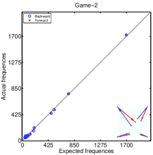
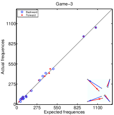
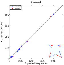
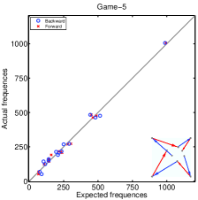
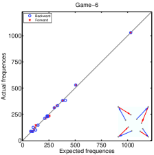
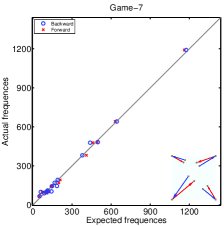
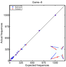
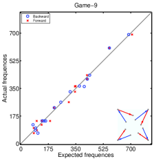
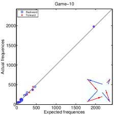
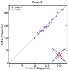
Figure 3: Comparison of the actual transition frequencies with expected transition frequencies in the experimental games. Horizonal axis is the expected transition frequencies from MaxEnt hypothesis; meanwhile, vertical axis is the actual transition frequencies. The first figure is the results of all 11 games. Figure 2$nd$ to last is for game 1 to game 11, respectively. In the first figure, symbol B (F) in the legend indicates backward (forward). For each game, there are four social states and 16 kinds of social forward transitions and 16 kinds of backward transitions. The cycles in blue (cross in red) indicate the backward transitions (forward transitions). A dot in diagonal line means the experimental transition frequencies equal to the theoretical transition frequencies. The sub-figures in the right down corners are the schematic diagrams for aggregated backward (forward) transitions in blue arrows (in red arrows).

The liner regression results are shown in Table5. Obliviously, each of the liner regression coefficients is very close to 1 and the $p<0.001$. Table5 also provides the $99\%$ C.I. (confidence interval) both for liner regression coefficients and intercept constant. All the lower bound of $99\%$ C.I. of regression coefficients are smaller than but very close to 1 and the upper bound are larger than but also very close to 1; then the equal hypothesis of the two variables can not be rejected. Meanwhile, for intercept constant (y-intercept, the point where a line crosses the y-axis), none of the $p$ value is smaller than 0.42, all of the lower bound of the $99\%$ C.I. are smaller than 0 and all of the upper bound are larger than 0. Then, the hypothesis that the regression line cross $0$ can not be rejected. These statistical results indicate that the hypothesis that theoretical values statistically equal to experimental observation of the transitions is supported.

In summary, in the laboratory experimental two-person constant sum 2$\times$2 games, the outcome of the social transitions fit MaxEnt. In another word, given the mean vector of the transitions of a given state, the distributions of the all transitions of the given state can be estimated with MaxEnt, and fit experiments data exactly.

Table 5: Results of linear regression for $T_{-}$ and $T_{+}$ of each game

	Coef. $T_{-}$†	[99%C.I]§	const. [99%C.I]‡	Coef. $T_{+}$†	[99%C.I]§	const. [99%C.I]‡
g1	1.019	0.971   1.067	-24.497   13.829	1.020	0.950    1.090	-33.665    22.369
g2	1.010	0.982   1.039	-17.453   11.596	1.012	0.983    1.041	-17.993    11.337
g3	0.995	0.943   1.047	-19.863   22.717	0.997	0.952    1.041	-17.420    19.273
g4	1.009	0.981   1.037	-14.445    9.388	1.013	0.978    1.048	-18.533    11.146
g5	1.005	0.922   1.088	-31.300   28.440	1.007	0.942    1.072	-25.466    21.471
g6	1.002	0.956   1.049	-17.457   16.123	1.003	0.961    1.045	-16.216    14.447
g7	1.012	0.954   1.070	-26.656   19.858	1.017	0.970    1.065	-23.895    14.080
g8	0.997	0.968   1.026	-11.762   13.329	1.000	0.974    1.026	-11.121    11.139
g9	1.009	0.909   1.110	-36.096   30.798	1.006	0.894    1.118	-38.853    35.654
g10	1.008	0.966   1.050	-24.502   20.038	1.009	0.972    1.045	-21.852    16.953
g11	1.002	0.886   1.119	-27.159   26.109	1.011	0.848    1.175	-39.890    34.780
total	1.007	0.995   1.019	-6.700    2.889	1.009	0.997    1.020	-7.170     2.317

• liner regression coefficient.

• 99$\%$ Confident Interval for liner regression coefficient.

• 99$\%$ Confident Interval for intercept constant.

VI Discussion and conclusion

The main result of this report is that, the social strategy transitions are not erratic but governed by MaxEnt suggested by Jaynes Jaynes1957 . This result comes from the dynamical observables in the experiments of human subject competing games RothErev2007 ; XuetalMaxEnt2012 .

VI.1 Examples of the Necessary of MaxEnt

To make the MaxEnt in social dynamics easier to understand, we provides two alternative examples in Fig. 2; The first example is in sub-figure (d), the backward transition distribution, which is consistent with the aggregated backward transition shown in (b) but not capture the experiment result in (a); In another word, in (d), the frequencies for $T_{00\leftarrow 01}$, $T_{00\leftarrow 00}$, $T_{00\leftarrow 10}$ and $T_{00\leftarrow 11}$ could be 133, 28, 0 and 271; Even though this distribution satisfied the constraint condition (b), it is far away from the experimental distribution in (a). Second example is for forward state transition in (h); without MaxEnt, a plausible distribution like the (h) in Fig. 2 does not provide efficient information of experimental dynamical observable in (e) with the constraint condition of (f). Alternatively, with MaxEnt, results in (c) and (g), by using (b) and (f) as the constraints, can recover the experimental distribution in (a) and (e), respectively.

VI.2 MaxEnt in social state transition and experimental social dynamics

In this section, we explain the connection of present results to the results found in experimental social dynamics.

The social dynamics of human subjects systems is an interdisciplinary field Friedman1998Rev ; social2009dynamics ; Sandholm2011 ; young2008stochastic . In this field, evolutionary game theory provides a general mathematical framework for the theoretical investigation of social dynamics and is used commonly by physicists and economics. However, this theory has rare gain the supports from laboratory experiments of human subject social systems quantitatively.

Only quite recently, according to the three reports from three independent research groups, quantitative experimental testing on evolutionary dynamics is becoming possible. The three reports are following. (1) The first is the report from Hoffman, Suetens, Nowak and Gneezy (2012) Nowak2012 . In three Rock-paper-scissors games, the authors compare behavior with three different symmetric matrices whose mean distances from identical Nash equilibrium (NE) are equal (unequal) in classical (evolutionary) game theory. They find the mean distance from NE in a treatment is larger which is predicted by replicator dynamics model in evolutionary game theory. This is the first experimental report to support one of the most fundamental concept — Evolutionarily stable state (ESS) — in evolutionary game theory. In their report, the simplest replicator dynamics model is used as a reference. (2) The second is the report from Cason, Friedman and Hopkins (2012) Friedman2012 . Using continuous time experiments, also in Rock-Paper-Scissors games, the authors found cycles directly. More Importantly, they found that the cycle amplitude, frequency and direction are consistent with standard learning models. In their report Friedman2012 , the logit dynamics model is used as a reference. Another important point is ”time” are served as controlled variable in their experiments. (3) The third are the report from Xu, Wang and Wang (2012) XuWangWang1208 . In two-population random-matched 2$\times$2 games with 12 different payoff-matrix parameters selten2008 , the experimental frequencies is found to be linear positive related to the theoretical frequencies significant ($>$5$\sigma$). The payoff-normalized replicator dynamics model is used as the reference. Together with the observed cyclic velocity vector field pattern in experiments XuWang2011ICCS , evidences from 2$\times$2 games support the evolutionary game theory as well. To test evolutionary dynamics in laboratory human subject social systems, these are the three experiments which are reported recently.

Notice that, all the three groups use accumulated observable (macro observable) to describe the social dynamics behaviors. In this letter, the macro observable which are used as the constraint conditions (e.g., the mean aggregated forward transition) are also macro observable. In this letter, we show that MaxEnt can provides more dynamics information (micro observable, the state-to-state transits) from the limited accumulated observable (macro observable) in the experiments.

In words, present report might provide a paradigm — the micro and macro dynamical observable could be linked by MaxEnt in social dynamical processes in experiments. We suggest the results reported in this letter could be replicated in more general conditions in the experiments of human subject social dynamics.

VI.3 MaxEnt as a Link between Nature and Social Science

In economics, MaxEnt approach has gained its widely applications, e.g., in market equilibrium Toda2010 ; Barde2012 , in wealth and income distribution Castaldi2007 ; WuMaxEntIncome2003 , in firm growth rates Alfarano2008 in behavior modeling Wolpert2012 . Theoretical interpreting or modeling of the distributions of social outcomes with MaxEnt is growing.

However, to the best of our knowledge, the dynamic behavior (both of the backward and forward transitions) obeys MaxEnt — this point has never been empirical presented. Our finding of the MaxEnt in dynamic behaviors in experimental data can be an encourage information for investigating the potential self-consistence of social outcome — both in static and dynamic performance.

MaxEnt, as a technique, can be used to predict the geographic distribution of any spatial phenomena, including plants and animals MaxEntSpecies2006 . In game theory condition, the spatial phenomena of social behavior is the phenomena in strategy space, at the same time, the absence or appearance of strategy is relative to the absence or appearance of species. This picture has been well built Sandholm2011 to unify the evolutionary theorems in biology science and social science. Our findings of the social behavior fitting MaxEnt, both in dynamic respect in this report and in static respect in XuetalMaxEnt2012 , suggest that human subject social systems and natural systems could have wider common backgrounds.

For the future investigations, several points need to be considered. As we have shown in static XuetalMaxEnt2012 and in one step ($x_{t\pm 1}$) dynamics social behaviors obey MaxEnt, dose any step transitions always obey MaxEnt? What is the bound of the MaxEnt in social interaction systems?

One can notice that, in the 11 games, all the social environments are different (for the payoff matrix are different), all the mixed strategy Nash equilibrium are different, however, all the social transitions obeying MexEnt are indifferent.

VI.4 Conclusion

By employing experimental economics data, we test the MaxEnt hypothesis in social transitions. In the experimental constant sum two-person 2$\times$2 games, the results show that, not only static social state distributions obey MaxEnt XuetalMaxEnt2012 , the distributions of the social state transitions also fit MaxEnt. This finding suggests that MaxEnt can also be an approach for the social dynamics.

Acknowledgment: Thanks to Alvin Roth for kindly providing us the data. This research was supported by the grant from the Experimental Social Science Laboratory of Zhejiang University (2012 annual project: The property of unstable equilibrium: an experimental investigation). We thank the anonymity reviewer for helpful suggestion. We also thank Zunfeng Wang for technical assistance, thank Shuang Wang and Yuqing Luo for polishing the English. All remaining errors belong to the authors.

References

- [1] S. Alfarano and M. Milakovic. Does classical competition explain the statistical features of firm growth? Economics Letters, 101(3):272–274, 2008.
- [2] S. Barde. Back to the future: economic rationality and maximum entropy prediction. Technical report, Department of Economics, University of Kent, 2012.
- [3] R. Battalio, L. Samuelson, and J. Van Huyck. Optimization incentives and coordination failure in laboratory stag hunt games. Econometrica, 69(3):749–764, 2001.
- [4] Jenna Bednar, Yan Chen, Tracy Xiao Liu, and Scott Page. Behavioral spillovers and cognitive load in multiple games: An experimental study. Games and Economic Behavior, 74(1):12–31, 2012.
- [5] M. Benaīm, J. Hofbauer, and E. Hopkins. Learning in games with unstable equilibria. Journal of Economic Theory, 144(4):1694–1709, 2009.
- [6] Y. Bereby-Meyer and A.E. Roth. The speed of learning in noisy games: partial reinforcement and the sustainability of cooperation. The American Economic Review, 96(4):1029–1042, 2006.
- [7] Timothy N. Cason, Anya C. Savikhin, and Roman M. Sheremeta. Behavioral spillovers in coordination games. European Economic Review, 56(2):233–245, 2012.
- [8] T.N. Cason, D. Friedman, and E. Hopkins. Cycles and instability in a rock-paper-scissors population game: a continuous time experiment. WP, 2012.
- [9] C. Castaldi and M. Milakovic. Turnover activity in wealth portfolios. Journal of economic behavior and organization, 63(3):537–552, 2007.
- [10] C. Castellano, S. Fortunato, and V. Loreto. Statistical physics of social dynamics. Reviews of Modern Physics, 81(2):591, 2009.
- [11] Y. Chen and R. Gazzale. When does learning in games generate convergence to nash equilibria? the role of supermodularity in an experimental setting. American Economic Review, pages 1505–1535, 2004.
- [12] Y Chen and FF Tang. Learning and incentive-compatible mechanisms for public goods provision: An experimental study. Journal of Political Economy, 106(3):633–662, 1998.
- [13] Y.W. Cheung and D. Friedman. A comparison of learning and replicator dynamics using experimental data. Journal of economic behavior and organization, 35(3):263–280, 1998.
- [14] I Erev, A.E. Roth, R.L. Slonim, and G Barron. Learning and equilibrium as useful approximations: Accuracy of prediction on randomly selected constant sum games. Economic Theory, 33(1):29–51, 2007.
- [15] A. Falk and J.J. Heckman. Lab experiments are a major source of knowledge in the social sciences. Science, 326(5952):535, 2009.
- [16] D. Friedman. Equilibrium in evolutionary games: Some experimental results. The Economic Journal, 106(434):1–25, 1996.
- [17] D. Friedman. Evolutionary economics goes mainstream: a review of the theory of learning in games. Journal of Evolutionary Economics, 8(4):423–432, 1998.
- [18] M. Hoffman, S. Suetens, M. Nowak, and U. Gneezy. An experimental test of nash equilibrium versus evolutionary stability. Science, submit, 2012.
- [19] E.T. Jaynes. Information theory and statistical mechanics. ii. Physical review, 108(2):171, 1957.
- [20] E.T. Jaynes and G.L. Bretthorst. Probability theory: the logic of science. Cambridge Univ Pr, 2003.
- [21] R.B. Myerson. Game theory: analysis of conflict. Harvard Univ Pr, 1997.
- [22] S.J. Phillips, R.P. Anderson, and R.E. Schapire. Maximum entropy modeling of species geographic distributions. Ecological modelling, 190(3):231–259, 2006.
- [23] W.H. Sandholm. Evolutionary Game Theory, pages 3176–3205. Springer New York, 2009.
- [24] W.H. Sandholm. Population games and evolutionary dynamics. MIT press, 2011.
- [25] Reinhard Selten and Thorsten Chmura. Stationary concepts for experimental 2x2-games. The American Economic Review, 98:938–966, 2008.
- [26] C.E. Shannon. A mathematical theory of communication. Bell System Technical Journal, page 535, 1948.
- [27] V.L. Smith. Theory, experiment and economics. The Journal of Economic Perspectives, 3(1):151–169, 1989.
- [28] A.A. Toda. Existence of a statistical equilibrium for an economy with endogenous offer sets. Economic Theory, 45(3):379–415, 2010.
- [29] J Van Huyck. Emergent conventions in evolutionary games. Handbook of Experimental Economics Results, 1:520–530, 2008.
- [30] David H. Wolpert, Michael Harr , Eckehard Olbrich, Nils Bertschinger, and J rgen Jost. Hysteresis effects of changing the parameters of noncooperative games. Physical Review E, 85(3):036102, 2012.
- [31] X. Wu. Calculation of maximum entropy densities with application to income distribution. Journal of Econometrics, 115(2):347–354, 2003.
- [32] B. Xu, S. Wang, and Z. Wang. Periodic frequencies of the cycles in 2 x 2 games. http://arxiv.org/abs/1208.6469v1, 2012.
- [33] B. Xu and Z. Wang. Evolutionary Dynamical Pattern of ”Coyness and Philandering”: Evidence from Experimental Economics, volume 3. p1313-1326, NECSI Knowledge Press, ISBN 978-0-9656328-4-3., 2011.
- [34] B. Xu and Z. Wang. Asymmetry spectrum of cycle amplitude in rock-paper-scissor game of experimental economics. http://dx.doi.org/10.2139/ssrn.2085459, 2012.
- [35] B. Xu and Z. Wang. Do cycles dissipate when subjects must choose simultaneously? http://arxiv.org/abs/1208.2396v1, 2012.
- [36] B. Xu, H. Zhang, Z. Wang, and J. Zhang. Test the principle of maximum entropy in constant sum 2x2 game: Evidence in experimental economics. Physics Letters A, http://dx.doi.org/10.1016/j.physleta.2012.02.047, 2012.
- [37] H.P. Young. Stochastic Adaptive Dynamics. New Palgrave Dictionary of Economics, revised edition, L. Blume and S. Durlauf, eds. Zanella, G.(2007), Discrete Choice with Social Interactions and Endogenous Membership, Journal of the European Economic Association, 5:122–153, 2008.