The Exact Smile of certain Local Volatility Models

Abstract

We introduce a new class of local volatility models. Within this framework, we obtain expressions for both (i) the price of any European option and (ii) the induced implied volatility smile. As an illustration of our framework, we perform specific pricing and implied volatility computations for a CEV-like example. Numerical examples are provided.

keywords: CEV, local volatility, stochastic volatility, implied volatility.

1 Introduction

Local volatility models are a class of equity models in which the volatility $\sigma_{t}$ of an asset $X$ is described by a function of time and the present level of $X$. That is, $\sigma_{t}=\sigma({}{t},X_{t})$. Among local volatility models, perhaps the most well-known is the constant elasticity of variance (CEV) model of Cox (1975). An extension of the CEV model to defaultable assets (the Jump-to-Default CEV or JDCEV model) is derived in Carr and Linetsky (2006). One advantage of these two local volatility models is that they admit closed-form pricing formulas for European options, written as infinite series of special functions. Another advantage of local volatility models is that, for models whose transition density is not available in closed form, accurate density approximations are often available. See, for example, Pagliarani and Pascucci (2011).

In this paper, we introduce a new class of local volatility models which, like the CEV and JDCEV models, allow for European option prices to be expressed in closed form as an infinite series. Additionally, we derive an expression for the exact implied volatility surface induced by our class of models. Previous studies of the implied volatility surface induced by local volatility models focused on heat-kernel expansions to derive asymptotic approximations of the volatility smile (see e.g., Gatheral et al. (2010); Henry-Labordère (2005) and references therein). It is worth mentioning that Dupire (1994) solves the inverse problem of finding a formula for the local volatility function the produces a given observed implied volatility surface exactly.

Essential for our mathematical presentation, is the use of spectral theory. The spectral representation theorem has been widely applied in mathematical finance. An exhaustive review would be prohibitive. However, we mention the seminal work of Davydov and Linetsky (2003), who lay the groundwork for option-pricing with eigenfunctions in a scalar diffusion setting. For applications of eigenfunction methods in a stochastic volatility (i.e., multivariate) setting, we refer the reader to Fouque et al. (2011); Lorig (2012a). While previous spectral-related work has focused exclusively on eigenfunction expansions for self-adjoint operators in Hilbert space, here, we focus on generalized eigenfunction expansions for normal operators. To our knowledge, this is the first time the spectral theory of normal operators has been used in a financial setting.

The rest of this paper proceeds as follows: in section 2 we present our class of models and describe our assumptions about the market. In section 3 we derive a formula for the price of a European option, written in a general form which is valid for any model within our framework. In section 4 we provide an formula for the implied volatility smile induced by our class models. In section 5, as an example of our framework, we perform explicit pricing and implied volatility computations for a CEV-like example. Numerical results are provided at the conclusion of the text. An appendix with some mathematical background is also provided. Concluding remarks can be found in section 6.

2 Model and assumptions

We assume a frictionless market, no arbitrage and take an equivalent martingale measure $\mathbb{P}$ chosen by the market on a complete filtered probability space $(\Omega,\mathscr{F},\{\mathscr{F}_{t},t\geq 0\},\mathbb{P})$. The filtration $\{\mathscr{F}_{t},t\geq 0\}$ represents the history of the market. All processes defined below live on this space. For simplicity we assume zero interest rates and no dividends so that all assets are martingales. We consider an asset $X$ whose dynamics are given by

$$dX_{t} =\left(a^{2}+\varepsilon\,\eta(\log X_{t})\right)^{1/2}X_{t}\,dW_{t},$$ (1)

where, $a>0$, $\varepsilon\geq 0$, the function $\eta:\mathbb{R}\to\mathbb{R}^{+}$ is an element of $\mathscr{S}$ (the Schwartz space of rapidly decreasing functions on $\mathbb{R}$; see equation (50) for a definition) and $W$ is a Brownian motion. The restriction $\eta\in\mathscr{S}$ is needed to prove Theorem 4. We assume that $X_{0}>0$, the initial value of $X$ is known. Note that $X$ has local volatility $\sigma(X_{t})=\left(a^{2}+\varepsilon\,\eta(\log X_{t})\right)^{1/2}$. Obviously, if $\eta=0$ then $X$ is a geometric Brownian motion. This will be key for the implied volatility analysis in section 4. Observe that both zero and infinity are natural boundaries according to Feller’s boundary classification for one-dimensional diffusions (see Borodin and Salminen (2002) pp. 14-15). That is, both zero and infinity are unattainable.

In what follows it will be convenient to introduce $Y=\log X$. A simple application of Itô’s formula shows that $Y$ satisfies

$$dY_{t} =-\frac{1}{2}\left(a^{2}+\varepsilon\,\eta(Y_{t})\right)dt+\left(a^{2}+\varepsilon\,\eta(Y_{t})\right)^{1/2}dW_{t}.$$ (2)

With $\eta\in\mathscr{S}$, the volatility and drift coefficients in (2) satisfy the usual growth and Lipschitz conditions, which guarantee a unique strong solution to SDE (2). See Øksendal (2005) Theorem 5.2.1.

3 Option pricing

We wish to find the time-zero value of a European-style option with payoff $h(Y_{t})$ at time $t>0$. Using risk-neutral pricing we express the initial value of the option $u^{\varepsilon}(t,y)$ as the risk-neutral expectation of the option payoff

$$u^{\varepsilon}(t,y) =\mathbb{E}_{y}\,h(Y_{t}), {}{(r=0)}$$ (3)

where the notation $\mathbb{E}_{y}$ indicates $\mathbb{P}$-expectation starting from $y=\log X_{0}$. Suppose $h\in C_{0}^{2}(\mathbb{R})$ (compactly supported functions with continuous derivatives up to order 2). Then, the function $u^{\varepsilon}(t,y)$ satisfies the Kolmogorov backward equation

$$\left(-\partial_{t}+\mathscr{A}^{\varepsilon}\right)u^{\varepsilon} =0, u^{\varepsilon}(0,y) =h(y).$$ (4)

where $\mathscr{A}^{\varepsilon}$ is the generator of the process $Y$. The domain of $\mathscr{A}^{\varepsilon}$ is defined as the set of $f$ for which the limit $\lim_{t\to 0}\frac{1}{t}\left(\mathbb{E}_{y}f(Y_{t})-f(y)\right)$ exists in the strong sense. For any $f\in C_{0}^{2}(\mathbb{R})$ the generator $\mathscr{A}^{\varepsilon}$ has the explicit representation

$$\mathscr{A}^{\varepsilon} =\mathscr{A}_{0}+\varepsilon\,\eta\,\mathscr{A}_{1}, \mathscr{A}_{0} =\frac{1}{2}a^{2}\left(\partial^{2}-\partial\right), \mathscr{A}_{1} =\frac{1}{2}\left(\partial^{2}-\partial\right),$$ (5)

where $\partial$, without the subscript $t$, indicates differentiation with respect to $y$.

Remark 1.

It is possible to extend our results to payoff functions $h$ that are continuous and have linear growth in $\log y$ (e.g. Call options). However, rigorous justification for this it outside the scope of this paper. Numerical tests are provided to support this claim.

Remark 2.

The operators $\mathscr{A}_{0}$ and $\mathscr{A}_{1}$ are normal operators in the Hilbert space $\mathscr{H}=L^{2}(\mathbb{R},dy)$ and satisfy the following (improper) eigenvalue equations (neither $\mathscr{A}_{0}$ nor $\mathscr{A}_{1}$ have any proper eigenvalues)

$$\mathscr{A}_{0}\psi_{\lambda} =\phi_{\lambda}\psi_{\lambda}, \psi_{\lambda} =\frac{1}{\sqrt{2\pi}}e^{i\lambda y}, \phi_{\lambda} =\frac{1}{2}a^{2}\left(-\lambda^{2}-i\lambda\right),$$ (6)

$$\mathscr{A}_{1}\psi_{\lambda} =\chi_{\lambda}\psi_{\lambda}, \psi_{\lambda} =\frac{1}{\sqrt{2\pi}}e^{i\lambda y}, \chi_{\lambda} =\frac{1}{2}\left(-\lambda^{2}-i\lambda\right).$$ (7)

Note that, as shown by Dirac (1927), for any analytic $f$, we have

$$\frac{1}{2\pi}\int_{\mathbb{R}}dx\,e^{-i\lambda x} =\delta(\lambda), \int_{\mathbb{R}}d\mu\,\delta(\lambda-\mu)f(\mu) =f(\lambda), \lambda \in\mathbb{C}.$$ (8)

Thus, the generalized eigenfunctions satisfy the orthogonality relation

$$(\psi_{\lambda},\psi_{\mu}) =\frac{1}{2\pi}\int_{\mathbb{R}}dx\,e^{-i(\lambda-\mu)x}=\delta(\lambda-\mu), \lambda,\mu \in\mathbb{C}.$$ (9)

See also, Friedman (1956), equation (4.35). Note also that Borel-measurable functions of normal operators (e.g., $g(\mathscr{A}_{0})$) are well-defined by the spectral theorem for normal operators, as explained in Appendix A.

We seek a solution to Cauchy problem (4) of the form

$$u^{\varepsilon} =\sum_{n=0}^{\infty}\varepsilon^{n}\,u_{n}.$$ (10)

We will justify this expansion in Theorem 4. Inserting the expansion (10) into Cauchy problem (4) and collecting terms of like powers of $\varepsilon$ we obtain

$$\mathscr{O}(1): (-\partial_{t}+\mathscr{A}_{0})u_{0} =0, u_{0}(0,y) =h(y),$$ (11)

$$\mathscr{O}(\varepsilon^{n}): (-\partial_{t}+\mathscr{A}_{0})u_{n} =-\eta\mathscr{A}_{1}u_{n-1}, u_{n}(0,y) =0.$$ (12)

The solution to the above equations is

$$\mathscr{O}(1): u_{0}(t,y) =e^{t\mathscr{A}_{0}}h(y),$$ (13)

$$\mathscr{O}(\varepsilon^{n}): u_{n}(t,y) =\int_{0}^{t}ds\,e^{(t-s)\mathscr{A}_{0}}\eta(y)\mathscr{A}_{1}u_{n-1}(s,y).$$ (14)

Using the equation (49) from appendix A to write the spectral representation of $e^{t\mathscr{A}_{0}}$ we obtain

$$\mathscr{O}(1): u_{0}(t,y) =\int_{\mathbb{R}}d\lambda\,e^{t\phi_{\lambda}}(\psi_{\lambda},h)\psi_{\lambda}(y),$$ (15)

$$\mathscr{O}(\varepsilon^{n}): u_{n}(t,y) =\int_{0}^{t}\int_{\mathbb{R}}ds\,d\mu\,e^{(t-s)\phi_{\mu}}\left(\psi_{\mu},\eta\mathscr{A}_{1}u_{n-1}(s,\cdot)\right)\psi_{\mu}(y),$$ (16)

After a bit of algebra, we find an explicit representation for $u_{n}(t,y)$

$$u_{n} =\underbrace{\int\cdots\int}_{n+1}\left(\prod_{k=0}^{n}d\lambda_{k}\right)\left(\sum_{k=0}^{n}\frac{e^{t\phi_{\lambda_{k}}}}{\prod_{j\neq k}^{n}(\phi_{\lambda_{k}}-\phi_{\lambda_{j}})}\right)\left(\prod_{k=0}^{n-1}\left(\psi_{\lambda_{k+1}},\eta\mathscr{A}_{1}\psi_{\lambda_{k}}\right)\right)\left(\psi_{\lambda_{0}},h\right)\,\psi_{\lambda_{n}}.$$ (17)

Remark 3.

As we will show in section 5, for certain choices of $\eta$, the $(n+1)$-fold integral in (17) will collapse into a single integral.

We have now obtained a formal expansion (10)-(17) for the price of a European option. The following theorem provides conditions under which the expansion is guaranteed to be valid.

Theorem 4.

Suppose $\varepsilon\leq\frac{a^{2}}{\left\|\eta\right\|}$, where $\left\|\eta\right\|=\sqrt{(\eta,\eta)}$. Then the option price $u^{\varepsilon}(t,y)$ is given by (10)-(17).

Proof.

See Appendix B.   ∎

4 Implied volatility

In this section we fix $(t,y)$ and a call option payoff $h(y)=(e^{y}-e^{k})^{+}$. Note that

$$(\psi_{\lambda},h) =\frac{-e^{k-ik\lambda}}{\sqrt{2\pi}\left(i\lambda+\lambda^{2}\right)}, \text{Im}(\lambda) <-1.$$ (18)

The following definitions will be useful:

Definition 5.

The Black-Scholes Price $u^{BS}:\mathbb{R}^{+}\to\mathbb{R}^{+}$ is defined as

$$u^{BS}(\sigma) :=\int_{\mathbb{R}}d\lambda\,e^{t\phi^{BS}_{\lambda}(\sigma)}(\psi_{\lambda},h)\psi_{\lambda}, \phi^{BS}_{\lambda}(\sigma) =\frac{1}{2}\sigma^{2}(-\lambda^{2}-i\lambda).$$ (19)

Remark 6.

Usually, the Black-Scholes price is written

$$u^{BS}(\sigma) =\int_{\mathbb{R}}dx\,h(x)\,\Phi_{m,s^{2}}(x), m =y-\frac{1}{2}\sigma^{2}t, s^{2} =\sigma^{2}t,$$ (20)

where $\Phi_{m,s^{2}}$ is a Gaussian density with mean $m$ and variance $s^{2}$. Equation (19) is simply the Fourier representation of (20).

Definition 7.

For each fixed $\log$ spot $y$, time to maturity $t$, and $\log$ strike price $k$, the Implied Volatility is defined implicitly as the unique number $\sigma^{\varepsilon}\in\mathbb{R}^{+}$ such that

$$u^{BS}(\sigma^{\varepsilon}) =u^{\varepsilon},$$ (21)

where $u^{\varepsilon}$ is as given in Theorem 4.

Remark 8.

Note that $u_{0}=u^{BS}(a)$. As shown in Lorig (2012b), when $u^{\varepsilon}$ can be expanded as an analytic series whose first term corresponds to $u^{BS}$, one can obtain the exact implied volatility corresponding to $u^{\varepsilon}$.

Remark 9.

For $0<t<\infty$ the existence and uniqueness of the implied volatility $\sigma^{\varepsilon}$ can be deduced by using the general arbitrage bounds for call prices and the monotonicity of $u^{BS}$. See Fouque et al. (2011), Section 2.1, Remark (i).

Remark 10.

Observe that, for any $\sigma_{0}>0$ and $\sigma_{0}+\delta>0$, the function $u^{BS}(\sigma_{0}+\delta)$ is given by its Taylor series:

$$u^{BS}(\sigma_{0}+\delta) =\sum_{n=0}^{\infty}\frac{\delta^{n}}{n!}\partial_{\sigma}^{n}u^{BS}(\sigma_{0}), \partial_{\sigma}^{n}u^{BS}(\sigma_{0}) =\int_{\mathbb{R}}d\lambda\,\left(\partial_{\sigma}^{n}e^{t\phi^{BS}_{\lambda}(\sigma_{0})}\right)(\psi_{\lambda},h)\psi_{\lambda}.$$ (22)

Observe also that, by monotonicity of $u^{BS}$ we have $\partial_{\sigma}u^{BS}(\sigma)>0$ for all $\sigma>0$. Therefore, $u^{BS}$ is an invertible analytic function. By the Lagrange inversion theorem, the inverse function $[u^{BS}]^{-1}$ is also analytic.

Clearly, $u^{\varepsilon}$ is an analytic function of $\varepsilon$ (we derived its power series expansion). It is a useful fact that the composition of two analytic functions is also analytic (see Brown and Churchill (1996), section 24, p. 74). Thus, in light of Remark 10, we deduce that $\sigma^{\varepsilon}=[u^{BS}]^{-1}(u^{\varepsilon})$ is an analytic function and therefore has a power series expansion in $\varepsilon$. We write this expansion as follows

$$\sigma^{\varepsilon} =\sigma_{0}+\delta^{\varepsilon}, \delta^{\varepsilon} =\sum_{k=1}^{\infty}\varepsilon^{k}\sigma_{k}.$$ (23)

Taylor expanding $u^{BS}$ about the point $\sigma_{0}$ we have

$$u^{BS}(\sigma^{\varepsilon}) =u^{BS}(\sigma_{0}+\delta^{\varepsilon})$$ (24)

$$=\sum_{n=0}^{\infty}\frac{1}{n!}(\delta^{\varepsilon}\partial_{\sigma})^{n}u^{BS}(\sigma_{0})$$ (25)

$$=u^{BS}(\sigma_{0})+\sum_{n=1}^{\infty}\frac{1}{n!}\left(\sum_{k=1}^{\infty}\varepsilon^{k}\sigma_{k}\right)^{n}\partial_{\sigma}^{n}u^{BS}(\sigma_{0})$$ (26)

$$=u^{BS}(\sigma_{0})+\sum_{n=1}^{\infty}\frac{1}{n!}\left[\sum_{k=1}^{\infty}\left(\sum_{j_{1}+\cdots+j_{n}=k}\prod_{i=1}^{n}\sigma_{j_{i}}\right)\varepsilon^{k}\right]\partial_{\sigma}^{n}u^{BS}(\sigma_{0})$$ (27)

$$=u^{BS}(\sigma_{0})+\sum_{k=1}^{\infty}\varepsilon^{k}\left[\sum_{n=1}^{\infty}\frac{1}{n!}\left(\sum_{j_{1}+\cdots+j_{n}=k}\prod_{i=1}^{n}\sigma_{j_{i}}\right)\partial_{\sigma}^{n}\right]u^{BS}(\sigma_{0})$$ (28)

$$=u^{BS}(\sigma_{0})+\sum_{k=1}^{\infty}\varepsilon^{k}\left[\sigma_{k}\partial_{\sigma}+\sum_{n=2}^{\infty}\frac{1}{n!}\left(\sum_{j_{1}+\cdots+j_{n}=k}\prod_{i=1}^{n}\sigma_{j_{i}}\right)\partial_{\sigma}^{n}\right]u^{BS}(\sigma_{0}).$$ (29)

Now, we insert expansions (10) and (29) into (21) and collect terms of like order in $\varepsilon$

$$\mathscr{O}(1): u_{0} =u^{BS}(\sigma_{0}),$$ (30)

$$\mathscr{O}(\varepsilon^{k}): u_{k} =\sigma_{k}\partial_{\sigma}u^{BS}(\sigma_{0})+\sum_{n=2}^{\infty}\frac{1}{n!}\left(\sum_{j_{1}+\cdots+j_{n}=k}\prod_{i=1}^{n}\sigma_{j_{i}}\right)\partial_{\sigma}^{n}u^{BS}(\sigma_{0}), k \geq 1.$$ (31)

Solving the above equations for $\{\sigma_{k}\}_{k=0}^{\infty}$ we find

$$\mathscr{O}(1): \sigma_{0} =a,$$ (32)

$$\mathscr{O}(\varepsilon^{k}): \sigma_{k} =\frac{1}{\partial_{\sigma}u^{BS}(\sigma_{0})}\left(u_{k}-\sum_{n=2}^{\infty}\frac{1}{n!}\left(\sum_{j_{1}+\cdots+j_{n}=k}\prod_{i=1}^{n}\sigma_{j_{i}}\right)\partial_{\sigma}^{n}u^{BS}(\sigma_{0})\right), k \geq 1.$$ (33)

Remark 11.

The right hand side of (33) involves only $\sigma_{j}$ for $j\leq k-1$. Thus, the $\{\sigma_{k}\}_{k=1}^{\infty}$ can be found recursively.

Explicitly, up to $\mathscr{O}(\varepsilon^{4})$ we have

$$\mathscr{O}(\varepsilon): \sigma_{1} =\frac{u_{1}}{\partial_{\sigma}u_{0}},$$ (34)

$$\mathscr{O}(\varepsilon^{2}): \sigma_{2} =\frac{u_{2}-\tfrac{1}{2}\sigma_{1}^{2}\partial_{\sigma}^{2}u_{0}}{\partial_{\sigma}u_{0}},$$ (35)

$$\mathscr{O}(\varepsilon^{3}): \sigma_{3} =\frac{u_{3}-(\sigma_{2}\sigma_{1}\partial_{\sigma}^{2}+\tfrac{1}{6}\sigma_{1}^{3}\partial_{\sigma}^{3})u_{0}}{\partial_{\sigma}u_{0}},$$ (36)

$$\mathscr{O}(\varepsilon^{4}): \sigma_{4} =\frac{u_{4}-(\sigma_{3}\sigma_{1}\partial_{\sigma}^{2}+\tfrac{1}{2}\sigma_{2}^{2}\partial_{\sigma}^{2}+\tfrac{1}{2}\sigma_{2}\sigma_{1}^{2}\partial_{\sigma}^{3}+\tfrac{1}{24}\sigma_{1}^{4}\partial_{\sigma}^{4})u_{0}}{\partial_{\sigma}u_{0}}.$$ (37)

We summarize our implied volatility result in the following theorem:

Theorem 12.

The implied volatility $\sigma^{\varepsilon}$ defined in (21) is given explicitly by (23) where $\sigma_{0}=a$ and $\{\sigma_{k}\}_{k=1}^{\infty}$ are given by (33).

Remark 13.

Everything we have done so far is exact. The accuracy of the implied volatility expansion (23) is limited only by the number of terms one wishes to compute.

5 CEV-like example

In the constant elasticity of variance (CEV) model of Cox (1975) the dynamics of $X$ are assumed to be of the form $dX_{t}=\sqrt{\varepsilon}\,X_{t}^{\beta/2}X_{t}dW_{t}$. A key feature of the CEV model is that, when $\beta<0$, the local volatility function $\sigma(x)=\sqrt{\varepsilon}\,x^{\beta/2}$ increases as $x\searrow 0$, which (i) is consistent with the leverage effect and (ii) results in a negative implied volatility skew. However, values of $\beta<0$ also cause the volatility to drop unrealistically close to zero as $x$ increases. If we choose $\eta(y)=e_{\beta}(y):=e^{\beta y}$ then from (1) the dynamics of $X$ become

$$dX_{t} =(a^{2}+\varepsilon X_{t}^{\beta})^{1/2}X_{t}dW_{t},$$ (38)

Note that the local volatility function $\sigma(x)=(a^{2}+\varepsilon\,x^{\beta})^{1/2}$ behaves asymptotically like $\sigma(x)\sim\sqrt{\varepsilon}\,x^{\beta/2}$ as $x\searrow 0$ and behaves asymptotically like a constant $\sigma(x)\sim a$ as $x\nearrow\infty$.

Remark 14.

Because $e^{\beta y}$ is unbounded as $y\to-\infty$ (recall $\beta<0$), the function $e_{\beta}\notin\mathscr{S}$. However, we can modify the domain of $u^{\varepsilon}(t,x)$ to be $\mathbb{R}^{+}\times\mathbb{R}_{0}$ where $\mathbb{R}_{0}:=(y_{0},\infty)$ and $y_{0}\in\mathbb{R}$ is arbitrary. The operators $\mathscr{A}_{0}$ and $\mathscr{A}_{1}$ would then be defined on $L^{2}(\mathbb{R}_{0},dy)$ and the domain of these operators would include an absorbing boundary condition at $y_{0}$ (signifying default of $X$ the first time $X$ reaches the level $e^{y_{0}}$). Note that $\left\|e_{\beta}\right\|_{0}:=(\int_{y_{0}}^{\infty}|e_{\beta}|^{2}dy)^{1/2}=e^{\beta y_{0}}/\sqrt{-2\beta}$. In the analysis that follows, it will simplify computations considerably if we continue to work on $L^{2}(\mathbb{R},dy)$ as working on $L^{2}(\mathbb{R}_{0},dy)$ would require modifying the eigenfunctions $\psi_{\lambda}$ from complex exponentials $\exp(i\lambda y)$ to sines $\sin(\lambda y)$. However, the simplification comes at a cost; in light of the conditions of theorem (4) our results may not be valid for values of $y<\frac{1}{\beta}\log\frac{a^{2}\sqrt{-2\beta}}{\varepsilon}$.

We wish to find a simplified expression for $u_{n}$ (17) for the case $\eta=e_{\beta}$. Using (7) and (9) we note that

$$(\psi_{\mu},e_{\beta}\mathscr{A}_{1}\psi_{\lambda}) =\chi_{\lambda}\,\frac{1}{2\pi}\int dx\,e^{i(\lambda-\mu-i\beta)x}=\chi_{\lambda}\,\delta(\lambda-\mu-i\beta).$$ (39)

Thus, the $(n+1)$-fold integral (17) collapses into a single integral

$$u_{n} =\int_{\mathbb{R}}d\lambda\left(\sum_{k=0}^{n}\frac{e^{t\phi_{\lambda-ik\beta}}}{\prod_{j\neq k}^{n}(\phi_{\lambda-ik\beta}-\phi_{\lambda-ij\beta})}\right)\left(\prod_{k=0}^{n-1}\chi_{\lambda-ik\beta}\right)(\psi_{\lambda},h)\,\psi_{\lambda-in\beta}$$ (40)

$$=e_{n\beta}\int_{\mathbb{R}}d\lambda\left(\sum_{k=0}^{n}\frac{e^{t\phi_{\lambda-ik\beta}}}{\prod_{j\neq k}^{n}(\phi_{\lambda-ik\beta}-\phi_{\lambda-ij\beta})}\right)\left(\prod_{k=0}^{n-1}\chi_{\lambda-ik\beta}\right)(\psi_{\lambda},h)\,\psi_{\lambda}.$$ (41)

Remark 15.

Although we have written the option price as an infinite series (10), from a practical standpoint, one is only able to compute $u^{\varepsilon}\approx{}{u^{(N)}:=}\sum_{n=0}^{N}\varepsilon^{n}u_{n}$ for some finite $N$. For any finite $N$ we may pass the sum $\sum_{n=0}^{N}$ through the integral appearing in (41). Thus, for the purposes of computation, the most convenient way express the approximate option price is

$$u^{\varepsilon} \approx{}{u^{(N)}=}\int_{\mathbb{R}}d\lambda\,(\psi_{\lambda},h)\,\psi_{\lambda}\sum_{n=0}^{N}\varepsilon^{n}\,e_{n\beta}\left(\sum_{k=0}^{n}\frac{e^{t\phi_{\lambda-ik\beta}}}{\prod_{j\neq k}^{n}(\phi_{\lambda-ik\beta}-\phi_{\lambda-ij\beta})}\right)\left(\prod_{k=0}^{n-1}\chi_{\lambda-ik\beta}\right).$$ (42)

Note, to obtain the approximate value of $u^{\varepsilon}$, only a single integration is required. This makes our pricing formula as efficient as other models in which option prices are expressed as a Fourier-type integral (e.g. exponential Lévy processes, Heston model, etc.).

Numerical Results

In light of Remarks 1, 14 and 15, we provide some numerical tests supporting the use of the model considered in section 5.

Monte Carlo Test

To text the accuracy of approximation (42), we compute the price of a series of European call options using approximation (42) with $N=10$. We then compute the price of the same series of call options by means of a Monte Carlo simulation using a standard Euler scheme with a time step of $10^{-3}$ years and $10^{7}$ sample paths. The largest relative error obtained in the Monte Carlo simulations (i.e., standard error divided by price) was $0.0012$. Finally, we convert call prices to implied volatilities by inverting Black-Scholes numerically. The results of this procedure are plotted in figure 1. The implied volatilities resulting from the two methods of computation are indistinguishable.

Convergence of Transition Density

Define the transition density $p^{\varepsilon}(t,y;y_{0})$ and the $\mathscr{O}(\varepsilon^{n})$ approximation of the transition density $p^{(n)}(t,y;y_{0})$, which are obtained by setting the payoff function $h$ equal to a Dirac delta function $h=\delta_{y}$. Explicitly

$$p^{\varepsilon}(t,y;y_{0}) =\mathbb{E}_{y_{0}}\,\delta_{y}(Y_{t}), p^{(n)}(t,y;y_{0}) =\sum_{k=0}^{n}\varepsilon^{k}p_{k}(t,y;y_{0}).$$ (43)

In order to test the rate of convergence of $p^{(n)}$ to $p^{\varepsilon}$, in figure 2, we plot the approximate transition density $p^{(n)}$ for different values of $n$. For $n\geq 6$ we see virtually no difference between $p^{(n)}$ and $p^{(n-1)}$.

Convergence of Implied Volatility

Finally, to see how well the implied volatility expansion of section 4 performs, we define the $\mathscr{O}(\varepsilon^{n})$ approximation of the implied volatility

$$\sigma^{(n)} :=\sum_{k=0}^{n}\varepsilon^{k}\sigma_{k},$$ (44)

$n=2$	$n=3$
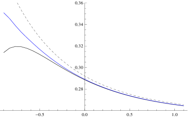
$n=4$	$n=5$

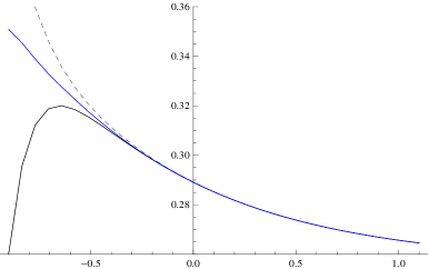
Figure 3: For different values of $n$, we plot $\sigma^{(n)}$ (solid black), $\sigma^{(n-1)}$ (dashed black) and $\sigma^{\varepsilon}$ (solid blue) as a function of LMMR. For $\text{LMMR}>-0.5$ we see fast convergence of $\sigma^{(n)}$ to $\sigma^{\varepsilon}$. For $\text{LMMR}<-0.5$, however, convergence is quite slow. Note that, although $\sigma^{(n)}$ appears to more closely approximate $\sigma^{\varepsilon}$ for odd $n$ than for even $n$, this is simply due to the fact that, for even $n$, $\sigma^{(n)}$ diverges downward, whereas for odd $n$, $\sigma^{(n)}$ diverges upward, matching the convexity of $\sigma^{\varepsilon}$. In fact, the region of convergence, loosely defined as the set of LMMR for which $\sigma^{(n)}$ closely approximates $\sigma^{\varepsilon}$, increases for every $n$. The following parameters are used in these plots: $a=0.25$, $\sqrt{\varepsilon}=0.15$, $\beta=-0.75$, $t=3.0$ $y=0.1$.

where the $\sigma_{k}$ are given by (33). In figure 3 we provide a numerical example illustrating convergence of $\sigma^{(n)}$ to $\sigma^{\varepsilon}$. We compute $\sigma^{\varepsilon}$ using a two-step procedure. First, we approximate $u^{\varepsilon}$ using (42) with $N=10$. In light of the Monte Carlo simulation above, this should introduce almost no error. Then, to find $\sigma^{\varepsilon}$, we solve $u^{BS}(\sigma^{\varepsilon})=u^{\varepsilon}$ numerically. Implied volatility is plotted as a function of the $\log$-moneyness to maturity ratio, $\text{LMMR}:=(k-y)/t$. Convergence is fastest for values of $k$ near $y$ and slows as $k$ moves away from $y$ in the negative direction.

6 Conclusion

In this paper we introduce a class of local stochastic volatility models. Within our modeling framework, we obtain a formula (written as an infinite series) for the price of any European option. Additionally, we obtain an explicit expression for the implied volatility smile induced by our class of models. As an example of our framework, we introduce a CEV-like model, which corrects one possible short-coming of the CEV model; namely, our choice of local volatility function does not drop to zero as the value of the underlying increases. Finally, in the CEV-like example, we show that option prices can be computed with the same level of efficiency as other models in which option prices are computed as Fourier-type integrals.

Thanks

The author would like to thank Bjorn Birnir and two anonymous reviewers for their helpful comments.

Appendix A Spectral theory of normal operators in a Hilbert space

In this appendix we briefly summarize the theory of normal operators acting on a Hilbert space. A detailed exposition on this topic (including proofs) can be found in Reed and Simon (1980) and Rudin (1973).

Let $\mathscr{H}$ be a Hilbert space with inner product $(\cdot,\cdot)$. The adjoint of an operator $\mathscr{A}$ acting in $\mathscr{H}$ is an operator $\mathscr{A}^{*}$ such that $(\mathscr{A}f,g)=(f,\mathscr{A}^{*}g)$. Here, for simplicity, we have assumed $\text{dom}(\mathscr{A})=\text{dom}(\mathscr{A}^{*})=\mathscr{H}$. An operator $(\text{dom}(\mathscr{A}),\mathscr{A})$ is said to be normal in $\mathscr{H}$ if it is closed, densely defined and commutes with its adjoint: $\mathscr{A}^{*}\mathscr{A}=\mathscr{A}\mathscr{A}^{*}$.

Suppose $\mathscr{A}$ is a normal operator acting on the Hilbert space $\mathscr{H}=L^{2}(\mathbb{R},dy)$. For any Borel measurable function $g$, the operator $g(\mathscr{A})$ can be constructed as follows. First, one solves the proper and improper eigenvalue problems

proper: $$\mathscr{A}\,\psi_{n} =\phi_{n}\,\psi_{n}, \phi_{n} \in\sigma_{d}(\mathscr{A}), \psi_{n} \in\mathscr{H},$$ (45)

improper: $$\mathscr{A}\,\psi_{\lambda} =\phi_{\lambda}\,\psi_{\lambda}, \phi_{\lambda} \in\sigma_{c}(\mathscr{A}), \psi_{\lambda} \notin\mathscr{H},$$ (46)

where $\sigma_{d}(\mathscr{A})$ and $\sigma_{c}(\mathscr{A})$ denote the discrete and continuous spectrum of $\mathscr{A}$, respectively. For the improper eigenvalue problem one extends the domain of $\mathscr{A}$ to include all functions $\psi$ for which $\mathscr{A}\psi$ makes sense and for which the following boundedness conditions are satisfied

$$\lim_{y\to\pm\infty}|\psi(y)|^{2} <\infty.$$ (47)

After normalizing, the proper and improper eigenfunctions of $\mathscr{A}$ satisfy the following orthogonality relations

$$\left(\psi_{n},\psi_{m}\right) =\delta_{n,m}, \left(\psi_{\lambda},\psi_{\lambda^{\prime}}\right) =\delta(\lambda-\lambda^{\prime}), \left(\psi_{n},\psi_{\lambda}\right) =0.$$ (48)

The operator $g(\mathscr{A})$ is then defined as follows (see Hanson and Yakovlev (2002), section 5.3.2)

$$g(\mathscr{A})f =\sum_{\phi_{n}\in\sigma_{d}(\mathscr{A})}g(\phi_{n})\left(\psi_{n},f\right)\psi_{n}+\int_{\sigma_{c}(\mathscr{A})}g(\phi_{\lambda})\left(\psi_{\lambda},f\right)\psi_{\lambda}d\lambda.$$ (49)

Appendix B Proof of Theorem 4

Our strategy is to show that $\mathscr{A}^{\varepsilon}=\mathscr{A}_{0}+\varepsilon\,\eta\,\mathscr{A}_{1}$ generates a semigroup $\mathscr{P}_{t}^{\varepsilon}=\exp(t\,\mathscr{A}^{\varepsilon})$. This will guarantee that $u^{\varepsilon}(t,y)=\mathscr{P}_{t}^{\varepsilon}h(y)$ is an analytic function of $\varepsilon$, which in turn, justifies the use of expansion (10). Throughout this section we will work on the Hilbert space $\mathscr{H}=L^{2}(\mathbb{R},dy)$. We let ${\rm dom}(\mathscr{A}_{i})=\mathscr{S}$, the Schwartz space of rapidly decreasing functions on $\mathbb{R}$:

$$\mathscr{S} =\{f\in C^{\infty}(\mathbb{R}):\left\|{f}\right\|_{\alpha,\beta}<\infty,\forall\,\alpha,\beta\}, \left\|{f}\right\|_{\alpha,\beta} =\sup_{y\in\mathbb{R}}|y^{\alpha}\partial^{\beta}f(y)|.$$ (50)

We note that $\mathscr{S}$ is a dense subset of $\mathscr{H}$. Thus, $\mathscr{A}_{i}$ has a unique extension $\overline{\mathscr{A}}_{i}$ with domain $\text{dom}(\overline{\mathscr{A}}_{i})=\mathscr{H}$. Our analysis begins with a Theorem from Chernoff (1972):

Theorem 16.

Let $\mathscr{A}$ be the generator of a $C_{0}$ contraction semigroup $\mathscr{P}_{t}^{0}=\exp(t\,\mathscr{A})$ on a Banach space. Let $\varepsilon\,\mathscr{B}$ be a dissipative operator with a densely defined adjoint. Assume that the inequality

$$\left\|{\varepsilon\,\mathscr{B}u}\right\| \leq c\left\|{u}\right\|+b\left\|{\mathscr{A}u}\right\|, \forall\,u \in{\rm dom}(\mathscr{A}),$$ (51)

holds for some $c\geq 0$ and $b\leq 1$ (i.e., the operator $\varepsilon\,\mathscr{B}$ is bounded relative to $\mathscr{A}$ with relative bound $b\leq 1$). Then the closure of $\mathscr{A}^{\varepsilon}:=\mathscr{A}+\varepsilon\,\mathscr{B}$ generates a $C_{0}$ contraction semigroup $\mathscr{P}_{t}^{\varepsilon}=\exp(t\,\mathscr{A}^{\varepsilon})$.

Remark 17.

Recall, an operator $\mathscr{A}$ is dissipative if $\text{Re}(u,\mathscr{A}u)\leq 0$ for all $u\in\mathscr{H}$.

Remark 18.

The operator $\mathscr{A}_{0}$ is the generator of a $C_{0}$ contraction semigroup $\mathscr{P}_{t}^{0}=\exp(t\,\mathscr{A}_{0})$ on $\mathscr{H}$. Thus, we must (i) show that $\varepsilon\,\eta\,\mathscr{A}_{1}$ has a densely defined adjoint, (ii) show that $\varepsilon\,\eta\,\mathscr{A}_{1}$ is dissipative and (iii) derive conditions under which $\varepsilon\,\eta\,\mathscr{A}_{1}$ is bounded relative to $\mathscr{A}_{0}$ with relative bound less than or equal to one.

To show (i) we note that the adjoint of $\varepsilon\,\eta\,\mathscr{A}_{1}$, given by $\left(\varepsilon\,\eta\,\mathscr{A}_{1}\right)^{*}=\varepsilon\,\mathscr{A}_{1}^{*}\,\eta$, has domain ${\rm dom}(\varepsilon\,\mathscr{A}_{1}^{*}\,\eta)=\mathscr{S}$. As mentioned above, $\mathscr{S}$ is densely defined in $\mathscr{H}$. To show (ii), we note that, if an operator satisfies the positive maximum principle then that operator is dissipative (see Ethier and Kurtz (1986), Lemma 4.2.1 on page 165). The following Theorem will be useful.

Theorem 19.

Let $\mathscr{A}$ be a linear operator with domain ${\rm dom}(\mathscr{A})=\mathscr{S}$. Then $\mathscr{A}$ satisfies the positive maximum principle if and only if

$$\mathscr{A} =\frac{1}{2}a^{2}(y)\partial^{2}+b(y)\partial+\int_{\mathbb{R}}\nu(y,dz)\left(e^{z\partial}-1-\mathbb{I}_{\{z<R\}}z\partial\right)-c(y),$$ (52)

for some $a(x)\geq 0$, $b(x)\in\mathbb{R}$, $c(x)\geq 0$, $R\in[0,\infty]$ and $\nu(y,dz)$ satisfying

$$\int_{\mathbb{R}}\nu(y,dz)\left(1\wedge z^{2}\right)<\infty.$$ (53)

Operators of the form (52) are called Lévy-type operators.

Proof.

See Theorem 2.12 of Hoh (1998).   ∎

The operator $\varepsilon\,\eta\,\mathscr{A}_{1}$ is clearly of the form (52). Hence, $\varepsilon\,\eta\,\mathscr{A}_{1}$ satisfies the positive maximum principle and is therefore dissipative. Finally, for part (iii), the following Theorem gives conditions under which $\varepsilon\,\eta\,\mathscr{A}_{1}$ is bounded relative to $\mathscr{A}_{0}$ with relative bound one.

Proposition 20.

Suppose $\varepsilon\leq\frac{a^{2}}{\left\|\eta\right\|}$ (which is the condition given in Theorem 4). Then $\varepsilon\,\eta\,\mathscr{A}_{1}$ is bounded relative to $\mathscr{A}_{0}$ with relative bound less than or equal to one.

Proof.

Clearly, for any $u\in{\rm dom}(\mathscr{A}_{0})$ we have

$$\left\|\varepsilon\,\eta\,\mathscr{A}_{1}\,u\right\| \leq\varepsilon\left\|\eta\right\|\cdot\left\|\mathscr{A}_{1}u\right\|=\frac{\varepsilon}{a^{2}}\left\|\eta\right\|\cdot\left\|\mathscr{A}_{0}u\right\|\leq\left\|\mathscr{A}_{0}u\right\|.$$ (54)

∎

The proof of Theorem 4 is complete.

Figure 1: We compute $u^{\varepsilon}$, the prices of set of European call options (i) by using approximation (42) with $N=10$ and (ii) by Monte Carlo simulation. We then convert the obtained prices to implied volatilities by inverting Black-Scholes numerically. The results of this procedure are plotted above. The green line corresponds to implied volatilities computed using approximation (42). The blue crosses corresponds to implied volatilities computed by Monte Carlo simulation. The units of the horizontal axis are $\log$-moneyness-to-maturity ratio $\text{LMMR}:=(k-y)/t$. The following parameters are used in these plots: $y=0.00$, $a=0.25$, $\sqrt{\varepsilon}=0.15$, $\beta=-0.75$, $t=1.0$. The two methods of computation produce indistinguishable implied volatilities.

$n=1$	$n=2$
$n=3$	$n=4$
$n=5$	$n=6$

Figure 2: A plot of the approximate transition density $p^{(n)}(t,y;0)$ for different values of $n$. In order to see convergence, we plot $p^{(n)}$ (solid) and $p^{(n-1)}$ (dashed) together. We see almost no difference between $p^{(5)}$ and $p^{(6)}$ (lower right). Note that the density of $Y_{t}$ has a fat tail to the left, which is expected since the local volatility function $\sigma(e^{y})=(a^{2}+\varepsilon e^{\beta y})^{1/2}$ increases as $y\to-\infty$. The following parameters are used in these plots: $a=0.20$, $\sqrt{\varepsilon}=0.15$, $\beta=-0.85$, $t=2.0$.

References

Borodin and
Salminen (2002)
Borodin, A. and P. Salminen (2002).
Handbook of Brownian motion: facts and formulae.
Birkhauser.
Brown and
Churchill (1996)
Brown, J. and R. Churchill (1996).
Complex variables and applications, Volume 7.
McGraw-Hill New York, NY.
Carr and
Linetsky (2006)
Carr, P. and V. Linetsky (2006).
A jump to default extended CEV model: An application of bessel
processes.
Finance and Stochastics10(3), 303–330.
Chernoff (1972)
Chernoff, P. R. (1972).
Perturbations of dissipative operators with relative bound one.
Proceedings of the American Mathematical Society33(1).
Cox (1975)
Cox, J. (1975).
Notes on option pricing I: Constant elasticity of diffusions.
Unpublished draft, Stanford University.
A revised version of the paper was published by the Journal of
Portfolio Management in 1996.
Davydov and
Linetsky (2003)
Davydov, D. and V. Linetsky (2003).
Pricing options on scalar diffusions: An eigenfunction expansion
approach.
Operations Research51(2), 185–209.
Dirac (1927)
Dirac, P. A. M. (1927).
The physical interpretation of the quantum dynamics.
Proceedings of the Royal Society of London. Series A, Containing
Papers of a Mathematical and Physical Character113(765), pp.
621–641.
Dupire (1994)
Dupire, B. (1994).
Pricing with a smile.
Risk7(1), 18–20.
Ethier and
Kurtz (1986)
Ethier, S. and T. Kurtz (1986).
Markov processes. characterization and convergence.
Fouque
et al. (2011)
Fouque, J.-P., S. Jaimungal, and M. Lorig (2011).
Spectral decomposition of option prices in fast mean-reverting
stochastic volatility models.
SIAM Journal on Financial Mathematics2(1).
http://www.pstat.ucsb.edu/faculty/fouque/.
Fouque et al. (2011)
Fouque, J.-P., G. Papanicolaou, R. Sircar, and K. Solna (2011).
Multiscale Stochastic Volatility for Equity, Interest-Rate and
Credit Derivatives.
Cambridge University Press.
Friedman (1956)
Friedman, B. (1956).
Principles and techniques of applied mathematics, Volume 280.
Wiley New York.
Gatheral et al. (2010)
Gatheral, J., E. Hsu, P. Laurence, C. Ouyang, and T. Wang (2010).
Asymptotics of implied volatility in local volatility models.
Mathematical Finance.
Hanson and
Yakovlev (2002)
Hanson, G. and A. Yakovlev (2002).
Operator theory for electromagnetics: an introduction.
Springer Verlag.
Henry-Labordère (2005)
Henry-Labordère, P. (2005).
A general asymptotic implied volatility for stochastic volatility
models.
Hoh (1998)
Hoh, W. (1998).
Pseudo differential operators generating markov processes.
Habilitations-schrift, Universität Bielefeld.
Lorig (2012a)
Lorig, M. (2012a).
Derivatives on multiscale diffusions: an eigenfunction expansion
approach.
To appear in Mathematical Finance.
Lorig (2012b)
Lorig, M. (2012b).
The exact volatility smile for exponential Lévy models.
Arxiv preprint arXiv:1207.0233.
Øksendal (2005)
Øksendal, B. (2005).
Stochastic Differential Equations: An Introduction with
Applications (6 ed.).
Springer-Verlag.
Pagliarani and
Pascucci (2011)
Pagliarani, S. and A. Pascucci (2011).
Analytical approximation of the transition density in a local
volatility model.
Central European Journal of Mathematics, 1–21.
Reed and
Simon (1980)
Reed, M. and B. Simon (1980).
Methods of modern mathematical physics. Volume I: Functional
Analysis.
Academic press.
Rudin (1973)
Rudin, W. (1973).
Functional analysis.
McGraw-Hill, New York.