Evolutionary Tracks of Trapped, Accreting Protoplanets: the Origin of the Observed Mass-Period Relation

Abstract

The large number of observed exoplanets ($\gtrsim$ 700) provides important constraints on their origin as deduced from the mass-period diagram of planets. The most surprising features in the diagram are 1) the (apparent) pile up of gas giants at a period of $\sim 500$ days ($\sim 1$ AU) and 2) the so-called mass-period relation which indicates that planetary mass is an increasing function of orbital period. We construct the evolutionary tracks of growing planets at planet traps in evolving protoplanetary disks and show that they provide a good physical understanding of how these observational properties arise. The fundamental feature of our model is that inhomogeneities in protoplanetary disks give rise to multiple (up to 3) trapping sites for rapid (type I) planetary migration of planetary cores. The viscous evolution of disks results in the slow radial movement of the traps and their cores from large to small orbital periods. In our model, the slow inward motion of planet traps is coupled with the standard core accretion scenario for planetary growth. As planets grow, type II migration takes over. Planet growth and radial movement are ultimately stalled by the dispersal of gas disks via photoevaporation. Our model makes a number of important predictions: that distinct sub-populations of planets that reflect the properties of planet traps where they have grown result in the mass-period relation; that the presence of these sub-populations naturally explains a pile-up of planets at $\sim 1$ AU; and that evolutionary tracks from the ice line do put planets at short periods and fill an earlier claimed ”planet desert” - sparse population of planets in the mass-semi-major axis diagram.

1. Introduction

The availability of large samples of exoplanets is being used to constrain theories of planet formation in a statistical sense (Udry & Santos 2007). The standard theoretical tools for this are the so-called population synthesis models (Ida & Lin 2004, 2008a; Mordasini et al. 2009; Ida & Lin 2010), wherein gas giants are considered to be formed by two main successive processes: the formation of cores by runaway (e.g. Wetherill & Stewart 1989) and oligarchic growth (e.g. Kokubo & Ida 1998), followed by gas accretion onto the cores (e.g. Pollack et al. 1996). This mode of forming gas giants is referred to as the core-accretion scenario. The orbits of these accreting protoplanets are regulated by planetary migration that eventually determines the radial distribution of planets (Ward 1997). The spirit of population synthesis models is to hypothesize that the diversity in the properties of observed exoplanets reflects the range of the (initial) disk environments in which planets are born. Fine tuning of the efficiency of various physical processes such as migration rates allows one to qualitatively reproduce the observations summarized in the mass-period diagram.

Despite the success of these models, a single complete theory of planet formation that can reproduce the architecture of any (exo)planetary system including our Solar system is still unknown. In particular, it is unclear as to the physical origin of several key observations: the (apparent) pile-up of planets at $\sim 1$ AU and the mass-period relation which shows that planetary mass increases with period (see Fig. 1). Furthermore, there is a significant discrepancy between the theories and observations: the recent population synthesis models claimed that a planet desert - a region in the mass-period diagram with a lower population of exoplanets - is present in the range of planetary mass ($5M_{\oplus}\lesssim M_{p}\lesssim 50M_{\oplus}$) and of their semi-major axis (0.04 AU$\lesssim r\lesssim$ 0.5 AU) (Ida & Lin 2004, 2008b) whereas many exoplanets are already observed there (see the black rectangle in Fig. 1).

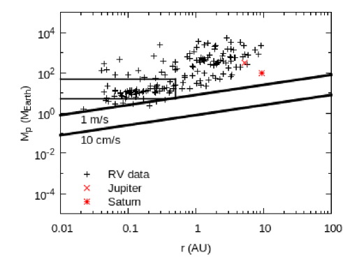
Figure 1.— Observed exoplanets using the radial velocity technique (denoted by black pluses). The data are obtained by the CORALIE and HARPS surveys, both of which are carried out through modest- and high-resolution spectrographs at La the Silla Observatory in Chile. We took the data from Mayor et al. (2011), wherein $\sim$ 150 observed exoplanets are selected from larger samples using consistent observational criteria for their statistical analyses. Thus, the data are well defined in order to discuss the statistical properties of exoplanets. Also, $M_{p}\sin i$ is plotted, since the inclinations $i$ are unknown. We have converted the data from orbital periods to semi-major axes for direct comparisons with our results (see Fig. 5). The host stars are F, G, or K stars. Jupiter (the red cross) and Saturn (the red star) are also shown for the reference. The thick black lines denote the amplitude of redial velocities of 1 m s^-1 and 10 cm s ^-1. The amplitude of 10 cm s ^-1 is not achieved yet even in the HARPS survey while 1 m s^-1 is well in hand. The data show the two trends; the (apparent) pile up of gas giants at $\sim 1$ AU and the mass-period relation wherein planetary mass is an increasing function of period (particularly beyond 1 AU). Earlier papers (Ida & Lin 2004, 2008b) predicted a planet desert demarcated by the black rectangle that covers in the range of planetary mass ($5M_{\oplus}\lesssim M_{p}\lesssim 50M_{\oplus}$) and of their semi-major axis (0.04 AU$\lesssim r\lesssim$ 0.5 AU) in the diagram. The recent observations populate the desert.

In this paper, we address how inhomogeneities in protoplanetary disks can account for the observed trends. For this purpose, we constructed and followed evolutionary tracks of planets that grow at disk inhomogeneities. More specifically, we compute planetary growth and migration in protoplanetary disks that evolve with time due to disk viscosity and photoevaporation of gas, by tracking the movement of disk inhomogeneities such as dead zones, ice lines and heat transitions. The fundamental contribution of disk inhomogeneities to theories of planet formation here is that they give rise to trapping sites for rapid type I planetary migration of cores of gas giants (often referred to as planet traps in the literature, Masset et al. 2006; Ida & Lin 2008b; Matsumura et al. 2009; Hasegawa & Pudritz 2010a; Lyra et al. 2010). Following the viscous evolution of disks, planet traps gradually move inwards in their disks, taking the trapped cores with them. The trapping and transport of cores is a central feature of our models in which protoplanets accrete gas as they move with the traps. We will show below that a semi-analytical model, wherein these two effects of planet traps, further planetary growth and subsequent type II migration that is terminated by photoevaporation of gas disks are all combined, can provide natural explanations of a number of the important observational properties: 1) the origin of the observed mass-period relation, 2) the origin of the pile up of observed gas giants at $\sim$ 1 AU, 3) the origin of low-mass planets distributing in the earlier claimed planet desert, 4) prediction of a new planet desert that originates from different physical processes than the earlier desert.

The plan of this paper is the following. In $\S$ 2, we summarize under what conditions planet traps are generated and which tidal torque and disk property play the most crucial role for activating the traps. In $\S$ 3, we describe disk models that are used for specifying the properties of disk inhomogeneities while, in $\S$ 4, we discuss how these inhomogeneities evolve with time following viscous evolution of disks with photoevaporation of gas. In $\S$ 5, we derive the characteristic masses of planets that are captured at planet traps and how these masses define the mode of planetary migration. In $\S$ 6, we synthesize the above treatments and develop a semi-analytical model of planetary growth and migration affected by planet traps for constructing evolutionary tracks of growing planets in the mass-period diagram. We present our results and compare them with the observations in $\S$ 7. The general reader may wish to skip to $\S$ 7 for a non-technical, astrophysical discussion of the results. Parameter studies are performed in $\S$ 8. $\S$ 9 is devoted to our discussion and conclusions.

2. Origins of planet traps

Planet traps, a term first coined by Masset et al. (2006), are one of the keys to resolving the long-standing problem of rapid type I migration that can lead to the loss of any planetary system to the host stars within $\sim 10^{5}$ years. This arises due to the high efficiency of angular momentum transfer between (proto)planets and their natal disks (Ward 1997; Tanaka et al. 2002). The basic idea of planet traps lies in the fact that the direction of migration can switch from inwards to outwards when planets migrate through the disks that have some kind of inhomogeneities. This is the combined consequence of the high sensitivity of type I migration to disk properties (Tanaka et al. 2002; Paardekooper et al. 2010; Hasegawa & Pudritz 2011a, b) and the density and temperature modifications produced by the disk inhomogeneities (D’Alessio et al. 1998; Menou & Goodman 2004; Matsumura et al. 2007; Hasegawa & Pudritz 2010b). Since a complete discussion of how disk inhomogeneities give rise to planet traps is presented elsewhere (e.g. Hasegawa & Pudritz 2011b, hereafter Paper I), we simply summarize the typical disk configurations with which planet traps are created and the responsible tidal torques and disk properties by which planet traps are activated with such disk configurations in Table 1. In this paper, we focus on dead zones, ice lines, and heat transitions which all become planet traps (see $\S$ 3 for their definitions, also see Paper I).

Table 1Typical disk structures for generating planet traps

Torque	Disk structures	Relevant disk properties
Lindblad torque	$t>1.5$ with $s=-1$	Dead zones
	$s<-2$ with $t=-0.5$	Dead zones and ice lines
Vortensity-related corotation torque	$s>1$ with $t\sim-0.5$	Inner edge of disks
Entropy-related corotation torque	$t<-1.1$ with $s=-1$	Viscous heating

Simple power-law disk structures are assumed, that is, the surface density of gas $\Sigma\propto r^{s}$ and the disk temperature $T\propto r^{t}$. We refer the reader to Paper I for a more complete discussion.

3. Disk models

A significant number of analytical and numerical studies have shown that ”realistic” disks are likely to possess several kinds of inhomogeneities (Gammie 1996; D’Alessio et al. 1998; Menou & Goodman 2004; Min et al. 2011), which can activate planet traps. We first briefly describe our disk models that serve as the basis for specifying the properties of the disk inhomogeneities such as their positions and surface densities. We refer the reader to Paper I for the complete discussion.

We adopt the standard models of steady accretion disks that have accretion rates modeled as

$$\dot{M}=3\pi\nu\Sigma_{g}=3\pi\alpha c_{s}H\Sigma_{g},$$ (1)

where $\Sigma_{g}$, $\nu=\alpha c_{s}H$, $c_{s}$, and $H$ are the surface density, the viscosity, the sound speed, and the pressure scale height of gas disks, respectively. The famous $\alpha-$prescription is assumed for characterizing the strength of disk turbulence (Shakura & Sunyaev 1973).

3.1. Positions of disk inhomogeneities

Adopting the standard disk model, we can estimate the positions of disk inhomogeneities. These positions are crucial because (proto)planets that undergo rapid type I migration will get trapped there. We simply summarize the positions here and refer the reader to Paper I for the complete derivations (also see Table 1).

There are generally of three kinds of disk inhomogeneities: dead zones, ice lines and heat transitions (Paper I). Dead zones are present in the inner region of disks where high energy photons such as X-rays from the central stars and cosmic rays cannot penetrate (Gammie 1996; Matsumura & Pudritz 2006; Ilgner & Nelson 2006). The defining feature of the dead zones is the low amplitude of turbulence there that results from the poor coupling of the magnetic field with weakly ionized disks (so that magnetorotational instabilities (MRIs) are suppressed there, e.g. Balbus 2003). Ice lines at which the disk temperature is low enough to trigger condensation of molecules such as water are the most famous and indispensable of disk inhomogeneities (Jang-Condell & Sasselov 2004; Min et al. 2011). They play an important role in population synthesis models (Ida & Lin 2004; Mordasini et al. 2009). Heat transitions are also well recognized in the literature and arise at that radius at which the main heat source changes from viscous heating to stellar irradiation (D’Alessio et al. 1998; Menou & Goodman 2004, Paper I). We have recently demonstrated that the heat transition becomes a planet trap based on analytical arguments (Paper I, also see Kretke & Lin 2012). The validity of the heat transition traps has been recently confirmed by hydrodynamic simulations (Yamada & Inaba 2012).

In principle, the structure of dead zones can be specified by solving the ionization equations (Sano et al. 2000; Matsumura & Pudritz 2006; Ilgner & Nelson 2006). Nonetheless, the resultant structures depend sensitively on disk parameters that are difficult to determine through the observations. Therefore, we adopt a parameterized treatment of dead zones (Kretke & Lin 2007; Ida & Lin 2008a; Matsumura et al. 2009, Paper I) in which the effective $\alpha$ in the layered region can be given as

$$\alpha=\frac{\Sigma_{A}\alpha_{A}+(\Sigma_{g}-\Sigma_{A})\alpha_{D}}{\Sigma_{g}},$$ (2)

where $\alpha_{A}$ and $\alpha_{D}$ are the strength of turbulence in the active and dead layers, respectively, and the surface density of the active layer $\Sigma_{A}$ is modeled as

$$\Sigma_{A}=\Sigma_{A0}f_{ice}\left(\frac{r}{r_{0}}\right)^{s_{A}},$$ (3)

where $r_{0}=1$ AU is the characteristic radius, $f_{ice}$ can contain the effects of ice lines. More specifically, $f_{ice}$ represents possible reductions of $\Sigma_{A}$ at the ice line that originate from the complex interplay between ice-coated, sticky dust grains and the absorption of free electrons by them (Sano et al. 2000; Ida & Lin 2008b, Paper I, see a more complete discussion). Thus, the structures of dead zones are controlled only by $\Sigma_{A0}$ and $s_{A}$ in this formalism. This approach is useful because it enables one to investigate how important the structure of dead zones is for understanding the population of planets by simply varying parameters, $\Sigma_{A0}$ and $s_{A}$ (see $\S$ 8). Assuming stationary disk models (see equation (1)), the surface density of gas is given as

$$\Sigma_{g}=\frac{\dot{M}}{3\pi c_{s}H\alpha_{D}}-\Sigma_{A}\frac{\alpha_{A}-\alpha_{D}}{\alpha_{D}}.$$ (4)

With equation (4) in hand, the position of a dead zone trap is given as

$$\frac{r_{dz}}{r_{0}}=\left(\frac{\dot{M}}{3\pi(\alpha_{A}+\alpha_{D})\Sigma_{A0}H_{0}^{2}\Omega_{0}}\right)^{\frac{1}{s_{A}+t+3/2}},$$ (5)

where $H_{0}$ and $\Omega_{0}$ are the pressure scale height and Keplerian frequency at $r=r_{0}$. This can be derived from the assumption that the outer edge of dead zones is specified around $\Sigma_{A}\sim\Sigma_{g}/2$.

The position of the ice line of molecular species $k$ is

$$\frac{r_{il}}{r_{0}}=\left[\frac{1}{T_{m,k}^{12}(r_{il})}\frac{27\bar{\kappa}_{0}\mu_{g}\Omega_{0}^{3}}{64\sigma_{SB}\alpha_{D}\gamma k_{B}}\left(\frac{\dot{M}}{3\pi}\right)^{2}\right]^{2/9}\propto\dot{M}^{4/9},$$ (6)

where $T_{m,k}$ is the disk midplane temperature below which molecules $k$ can condense, $\bar{\kappa}_{0}=2\times 10^{16}$ is the opacity at the ice line of the molecule, $\mu_{g}$ is the mean molecular weight of the gas, $k_{B}$ is the Boltzmann constant, and $\gamma=1.4$ is the adiabatic index. This is given by the recent results which show that the viscous heating (rather than stellar irradiation) is generally dominant for determining the position of ice lines (Min et al. 2011, Paper I). This expression is applicable for any molecules. Nonetheless, we focus on water ice lines here, since they are likely to be the most important molecule for understanding the observed mass-period relation (Paper I). For ice lines of water, $T_{m,\mbox{H}_{2}\mbox{O}}(r_{il})=170$ K (Jang-Condell & Sasselov 2004).

For the case that ice lines are located within dead zones, the position of the trap needs to satisfy the following condition:

$$\frac{r_{il}}{r_{dz}}>\left(h(r_{dz})\frac{\alpha_{A}+\alpha_{D}}{\alpha_{A}-\alpha_{D}}\right)^{\frac{1}{s_{A}+t/2+1}}.$$ (7)

Finally, the position of heat transitions is written as

$$\frac{r_{ht}}{r_{0}} = \left[\frac{1}{T_{m0}}\left(\frac{r_{0}}{R_{*}}\right)^{3/7}\left(\frac{27\bar{\kappa}_{0}\mu_{g}\Omega_{0}^{3}}{64\sigma_{SB}\alpha_{A}\gamma k_{B}}\left(\frac{\dot{M}}{3\pi}\right)^{2}\right)^{1/3}\right]^{14/15}$$

$$\propto \dot{M}^{28/45},$$

where $\bar{\kappa}_{0}=2\times 10^{-4}$ is the opacity at the heat transitions, $R_{*}$ is stellar radius,

$$T_{m0}\simeq\left(\frac{1}{H}\right)^{2/7}\left(\frac{T_{*}}{T_{c}}\right)^{1/7}T_{*},$$ (9)

$$T_{c}\equiv\frac{GM_{*}\mu_{g}}{k_{B}R_{*}},$$ (10)

$T_{*}$ and $M_{*}$ are stellar effective temperature and mass, respectively, and $G$ is the gravitational constant. We have adopted analytical models of Chiang & Goldreich (1997) for the temperature of the disk midplane heated by stellar irradiation. Planet traps arising from the heat transitions are active only if $r_{ht}>r_{dz}$.

By comparing the positions of each disk inhomogeneity (see equations (5), (6), and (3.1)), one immediately observes that disk evolution, which lowers the accretion rate $\dot{M}$, moves them inwards, but at different rates (see Fig. 2). This is important for understanding the observed mass-period relation.

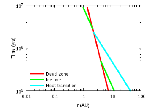
Figure 2.— Time evolution of the positions of three disk inhomogeneities for a disk around a classical T Tauri star (CTTS). The dead zone is denoted by red, the ice line by green, and the heat transition by light blue. Following the viscous evolution of disks, these zones move inwards at different rates. This results in the complex behaviors; convergence, disappearance, and re-appearance. Their end points are determined when photoevaporation of the gas disk takes place.

3.2. Characteristic surface densities at disk inhomogeneities

We estimate the characteristic surface densities at the disk inhomogeneities, following the above formulation. Although the detailed structures of disk inhomogeneities remain to be simulated, a number of analytical and numerical studies based on the standard viscous disk theory clarified their characteristic structure (Menou & Goodman 2004; Matsumura et al. 2007; Ida & Lin 2008b). These surface densities are utilized for deriving the characteristic masses of planets and following evolutionary tracks of planets that grow in planet traps.

As briefly mentioned above, the outer edge of dead zones is determined by $\Sigma_{A}\sim\Sigma_{g}/2$. Substituting this condition into equation (4), we find that the characteristic surface density at $r_{dz}$ is given as

$$\Sigma_{g,dz}\approx\frac{2\dot{M}}{3\pi(\alpha_{A}+\alpha_{D})r^{2}h^{2}\Omega},$$ (11)

where $h=H/r$ is the aspect ratio.

At the ice lines, the surface density is approximately written as

$$\Sigma_{g,il}\approx\frac{\dot{M}}{3\pi\alpha_{D}r^{2}h^{2}\Omega}.$$ (12)

We took the mean value of $\alpha$ as $\sim\alpha_{D}$. As mentioned before, this assumption is based on the recent extensive studies of ice lines (Sano et al. 2000; Ida & Lin 2008b, Paper I). These studies indicate that ice lines can be regarded as a localized dead zone.

On the other hand, the magnitude of turbulence at the heat transition is expected to be high enough to assume that disks are fully turbulent. As a result, the characteristic surface density at the heat transitions is given as

$$\Sigma_{g,ht}\approx\frac{\dot{M}}{3\pi\alpha_{A}r^{2}h^{2}\Omega}.$$ (13)

4. Time evolution of disks and their inhomogeneities

Time evolution of protoplanetary disks is established by the combination of viscous turbulence and the photoevaporation of gas. These agents regulate the movement of disk inhomogeneities. We present our treatments of them.

4.1. Viscous evolution

Viscous turbulence is the dominant driver of disk evolution (e.g. Armitage 2011). We adopt similarity solutions (Lynden-Bell & Pringle 1974) for constraining the relation between the accretion rate $\dot{M}$ and time $\tau$. Similarity solutions are derived from the conservation of angular momentum of disks (also see Hartmann et al. 1998). Considering a disk that has mass $M_{d}$ and a characteristic disk radius $R_{c}$, its angular momentum $J_{d}$ can be written as

$$J_{d}\approx M_{d}R_{c}^{1/2}.$$ (14)

Following time evolution where disk material is accreted onto the central star, equation (14) ensures that $R_{c}$ is an increasing function of time (since $J_{d}$ is roughly constant and $M_{d}$ steadily decreases with time). In a simplified analysis, the expansion rate of $R_{c}$ can be written as

$$\frac{dR_{c}}{dt}\approx\frac{R_{c}}{\tau_{vis}},$$ (15)

where $\tau_{vis}=r^{2}/(3\nu)$ is the viscous timescale. Assuming a power-law structure for the disk temperature ($T\propto r^{t}$), equation (15) gives

$$R_{d}\propto\tau^{\frac{1}{(1/2-t)}},$$ (16)

and the total disk mass $M_{d}$ decreases as (see equation (14))

$$M_{d}\propto\tau^{-1/(1-2t)}.$$ (17)

As a result, the accretion rate is related to time through the following relation;

$$\dot{M}\propto\tau^{-\frac{t-1}{t-1/2}}.$$ (18)

Combining the observations which show that the median accretion rate for classical T Tauri stars (CTTSs) of age $\sim 1$ Myrs is $\sim 10^{-8}M_{\odot}$ yr^-1 (Hartmann et al. 1998) and that $\dot{M}\propto M_{*}^{2}$ (Calvet et al. 2004; Muzerolle et al. 2005), we have the following scaling law for accretion rates;

$$\dot{M}\simeq 10^{-8}M_{\odot}\mbox{ yr}^{-1}f_{acc}\left(\frac{\tau}{10^{6}\mbox{ yr}}\right)^{-\frac{t-1}{t-1/2}}\left(\frac{M_{*}}{0.5M_{\odot}}\right)^{2},$$ (19)

where we have assumed that the typical mass of CTTSs is $\sim 0.5M_{\odot}$ and introduced a dimensionless factor $f_{acc}$. This factor can be utilized for varying $\dot{M}$ and investigating the subsequent consequences on disk evolution and planet formation.

4.2. Photoevaporation

It is still unclear how gas disks disperse in the final stages of their evolution (e.g. Armitage 2011). One of the leading mechanisms is photoevaporation which arises from heating up gas by high energy photons from the surrounding stars and subsequent evaporation of gas due to the thermal pressure (Hollenbach et al. 1994; Johnstone et al. 1998). In principle, photoevaporation rates are determined by the complex interplay between physical and chemical processes that take place in protoplanetary disks being irradiated by their central and nearby massive stars from far-UV (FUV) to extreme-UV (EUV) and up to X-rays (Gorti & Hollenbach 2009, references herein). Recent extensive studies have investigated how effective photoevaporation is in the dispersal of gas disks. In our models, we adopt a simple scaling law to represent the effects of photoevaporation.

Following the treatment of Adams et al. (2004, see their Appendix for the complete derivation), photoevaporation rates can be scaled as

$$\dot{M}_{pe}=f_{pe}N_{C}\mu_{g}c_{s}r_{g}\left(\frac{r_{g}}{r}\right)\exp\left(-\frac{r_{g}}{2r}\right),$$ (20)

where $f_{pe}$ is a dimensionless factor of order unity, $N_{C}$ is the critical column density of gas that is heated by stellar radiation, and the gravitational radius $r_{g}$ is given as

$$r_{g}=\frac{GM_{*}\mu_{g}}{k_{B}T}\approx 100\mbox{ AU}\left(\frac{T}{1000\mbox{ K}}\right)^{-1}\left(\frac{M_{*}}{1M_{\odot}}\right).$$ (21)

Utilizing some of the most advanced results of photoevaporation, we further simplified equation (20). Recently, Gorti & Hollenbach (2009) have investigated photoevaporation of gas disks by taking into account radiation of a central star that covers FUV, EUV and X-rays, and found that FUV heating plays the dominant role for inducing photoevaporation at $r\gtrsim$ 3 AU. This can be understood by the fact that photoevaporation rates are determined by the product of the gas temperature and density. EUV heating that leads to ionizing atomic hydrogen results in higher gas temperatures ($\sim 10^{4}$ K) than FUV heating ($\sim 10^{2}-10^{3}$ K). Nonetheless, the ionization front above which EUV heating dominates can only penetrate the disk atmosphere where gas density is much lower than that where FUV heating becomes dominant. As a result, FUV-induced photoevaporation rates exceed EUV-induced ones.

When photoevaporation is established mainly by FUV heating, the heated outgoing flow acts as an additional source of opacity for the FUV photons (Johnstone et al. 1998; Adams et al. 2004). Consequently, the critical column density heated up by FUV satisfies the self-regulation relation;

$$\tau_{FUV}=\sigma_{FUV}N_{C}\sim 1,$$ (22)

where $\sigma_{FUV}\approx 8\times 10^{-22}$ cm² is the reasonable cross section of dust grains for the FUV photons. This enables us to specify $N_{C}$ in equation (20). Also, the peak of FUV-induced photoevaporation rates is attained around 0.1-0.2$r_{g}$, rather than $r_{g}$ that is valid for EUV-induced photoevaporation (Adams et al. 2004; Gorti & Hollenbach 2009). This can be again explained by the combination of the gas temperature and density, and is also confirmed by equation (20).

Collecting the above arguments, we obtain a simplified, but physically motivated scaling law for photoevaporation rates;

$$\dot{M}_{pe}\simeq 2.3\times 10^{-9}M_{\odot}\mbox{ yr}^{-1}f_{pe}\left(\frac{c_{s}}{3\mbox{ km s}^{-1}}\right)^{-1}\left(\frac{M_{*}}{1M_{\odot}}\right),$$ (23)

where we have used equations (21) and (22) and set that $r=0.1r_{g}$ in equation (20).

We note that equation (23) can be applied for photoevaporation rates induced by both EUV and X-rays despite the fact that it is derived from the physical consideration based on FUV radiation. This can be done by adjusting the dimensionless factor $f_{pe}$ that is determined by the comparison with more detailed simulations. In fact, the conclusion of Gorti & Hollenbach (2009) that FUV is the dominant source of photoevaporation is still a matter of debate in the literature. This is partly because they relied exclusively on hydrostatic solutions for quantifying winds driven by FUV radiation (although hydrodynamical models are needed for precisely estimating the winds), and partly because they adopted energy spectra which eventually reduce the effects of X-rays. As shown by Owen et al. (2010, 2011, 2012), photoevaporation rates induced by X-rays can attain $\sim 10^{-8}$ M_⊙ yr^-1 for the most luminous X-ray sources. This high value is derived from employing observed Chandra spectra of TTSs and is comparable to the photoevaporation rate induced by FUV radiation. As a result, we intentionally avoid specifying the dominant source of photoevaporation of gas. Instead, we consider the general effects of photoevaporation on planet formation by treating $f_{pe}$ as a free parameter.

4.3. Photoevaporation of viscous disks

We are now in the position to discuss the complete treatment of disk evolution. We assume that the accretion rate through the disk is constant in space and regulated in time by equation (19). As time goes on, disk material accretes onto the central star and the accretion rate decreases. This change in $\dot{M}$ drives the movement of the disk inhomogeneities (see equations (5), (6), and (3.1)). When $\dot{M}$ becomes equal to the photoevaporation rate $\dot{M}_{pe}$, represented by equation (23), we assume the gas disks to disperse completely. Although this treatment is somewhat idealized, it can account for the more detailed simulations. As an example, Gorti et al. (2009) investigated the evolution of viscous protoplanetary disks that are photoevaporated by the FUV, EUV, and X-ray radiation from their central star. They showed that viscous turbulence controls the early stage of disk evolution and the total disk mass gradually decreases initially, which can be formulated by power-laws. Once the condition that $\dot{M}\sim\dot{M}_{pe}$ is satisfied, the disk mass drops exponentially due to the combination of viscous evolution and photoevaporation of gas. They found that disks of initial mass $0.1M_{\odot}$ around $\sim 1M_{\odot}$ have the lifetime of $\sim 4\times 10^{6}$ years.

We can derive similar results from our treatment by equating $\dot{M}$ with $\dot{M}_{pe}$: the disk lifetime is approximately estimated as $\sim 6\times 10^{6}$ years. Thus, our treatment is sufficient for the purpose of representing the evolution of protoplanetary disks that are regulated by both viscosity and photoevaporation.

In summary, we reduce the surface density of gas and the accretion rates, following equation (19). This results in the movement of the disk inhomogeneities. Also, we locate the final position of each disk inhomogeneity that is determined by the condition that $\dot{M}=\dot{M}_{pe}$.

4.4. Parameters

We summarize important parameters that establish the configuration and physical state of protoplanetary disks (see Table 2). They are divided into three sets: stellar parameters ($M_{*}$, $T_{*}$, and $R_{*}$), the disk mass ($\Sigma_{A0}$, $s_{A}$, $f_{acc}$, and $t$), and disk evolution ($\alpha_{A}$, $\alpha_{D}$, and $f_{pe}$). The disk evolution parameters can be translated into disk lifetimes. These three sets are fundamental to regulate planet formation in the disks, as confirmed in the population synthesis models (Ida & Lin 2004; Mordasini et al. 2009). We focus on disks around CTTSs and denote the set of the values given in Table 2 as our fiducial model. Adopting these parameters, disk evolution proceeds from $\tau_{int}=10^{5}$ year to the time at $\dot{M}=\dot{M}_{pe}$ that defines the disk lifetime ($\tau_{disk}$). A parameter study in which some of these quantities are changed is presented in $\S$ 8.

Table 2Important disk quantities

Symbols	Meaning	CTTSs
$M_{*}$	Stellar mass	0.5 $M_{\odot}$
$R_{*}$	Stellar radius	2.5 $R_{\odot}$
$T_{*}$	Stellar effective temperature	4000 K
$\Sigma_{A0}$	Surface density of active regions at $r=r_{0}$	20 g cm-2
$s_{A}$	Power-law index of $\Sigma_{A}(\propto r^{s_{A}})$	3
$t$	Power-law index of the disk temperature ($T\propto r^{t}$)	-1/2
$f_{acc}$	a dimensionless factor for $\dot{M}$ (see equation (19))	1
$\alpha_{A}$	Strength of turbulence in the active zone	$10^{-3}$
$\alpha_{D}$	Strength of turbulence in the dead zone	$10^{-4}$
$f_{pe}$	a dimensionless factor for $\dot{M}_{pe}$ (see equation (20))	1/3

4.5. Movement of planet traps

We draw upon our comprehensive analytical study (Paper I) which showed that the gas surface density and temperature modifications induced by the disk inhomogeneities are significant enough to reverse the direction of rapid type I migration. Therefore these positions are indeed trapping points of rapid type I migrators.

Fig. 2 shows the movement of all the three disk inhomogeneities. As demonstrated by Paper I, they all move inwards, but at different rates. The inward movements arise from the viscous evolution and the resultant reduction of the surface density of the disks (see equation (19)). Also, different moving rates for the traps result in complex behaviors of the multiple inhomogeneities such as convergence (e.g. merging of the heat transition with the dead zone), disappearance, and re-emergence of inhomogeneities (e.g. the behavior of the ice line). When $\dot{M}$ equals $\dot{M}_{pe}$, photoevaporation quickly disperses gas in the disk and hence the movement of the planet traps is terminated. This also determines the lifetime of the disk which is $\sim 8.8\times 10^{6}$ years in this configuration. The behavior of the planet traps is crucial for understanding the observed mass-period relation later.

5. Characteristic masses

We describe four characteristic masses that are important in our models (see Table 3). Using the positions and characteristic surface densities at disk inhomogeneities given in $\S$ 3, these masses define the mode of planetary migration (see $\S$ 6). Also, they result in a segment of the mass-semi-major axis diagram (see Appendix A).

Table 3Characteristic masses

Symbols	Meaning	Equation
$M_{mig,I}$	Minimum mass of type I migrators	(27)
$M_{gap}$	Gap-opening mass	(28)
$M_{crit}$	Critical mass of type II migrators	(29)
$M_{max}$	Maximum mass of planets	(5.3)

5.1. Type I regime

For planets of mass smaller than the gap-opening mass $M_{gap}$ (see below), type I migration is the main agent that governs their orbital distribution. In our models, rapid type I migration is halted at the planet traps. Hence the location of type I migrators is predicted by the positions of disk inhomogeneities (Paper I, see Fig. 2).

It is important to define the minimum mass of planets that will be captured by the planet traps. As demonstrated numerically by Lyra et al. (2010), planets captured in planet traps ”drop-out” if the following condition is satisfied:

$$\frac{\tau_{mig,I}}{\tau_{\nu}}>1,$$ (24)

where $\tau_{mig,I}$ is the timescale of type I planetary migration and $\tau_{\nu}$ is the timescale that determines the moving rates of planet traps. This relation expresses the fact that trapped planets drop-out if the speed of type I migration becomes less than that of the moving traps. In general, $\tau_{mig,I}$ is scaled as

$$\tau_{mig,I}=\frac{M_{p}r_{p}^{2}\Omega_{p}}{2\Gamma},$$ (25)

where

$$\Gamma=K_{mig}\left(\frac{M_{p}}{M_{*}}\right)^{2}\frac{\Sigma_{g,p}r_{p}^{4}\Omega_{p}^{2}}{h_{p}^{2}}$$ (26)

with $K_{mig}=1-10$, depending on the optical thickness of the disk (Paardekooper et al. 2010). For stationary accretion disk models (see equation (1)), the minimum mass of type I migrators that can be captured at planet traps is given as

$$M_{mig,I}=\frac{h_{p}^{2}M_{*}^{2}}{2K_{mig}\Sigma_{g,p}r_{p}^{2}\Omega_{p}\tau_{\nu}}.$$ (27)

We set $\tau_{\nu}=10^{6}$ yrs, because the moving rates of planet traps are eventually regulated by disk lifetimes (see Fig. 2) and the observations revealed that the disk lifetime of any CTTS disk is an order of Myrs.

5.2. Gap-opening mass

The gap-opening mass $M_{gap}$ distinguishes type I migration from type II and is well discussed in the literature (e.g. Ward 1997; Matsumura & Pudritz 2006). It arises when a planet becomes sufficiently massive that the torque it exerts on the disk opens a gap. There are two main arguments for estimating $M_{gap}$. The first one is the Hill radius analysis: the Hill radius should be larger than the pressure scale height for maintaining gap formation, otherwise gaps are closed by the gas pressure. The second argument arises from viscous disks. Disk viscosity that controls disk evolution plays the counteractive role for gap formation. Therefore, the tidal torque of a planet on their disks opens a gap if it exceeds the viscous torque. Summarizing these arguments, $M_{gap}$ is given as (e.g. Matsumura & Pudritz 2006)

$$\frac{M_{gap}}{M_{*}}=\mbox{min}\left[3h_{p}^{3},\sqrt{40\alpha h_{p}^{5}}\right].$$ (28)

5.3. Type II regime

Planets of mass larger than $M_{gap}$ open up a gap in their disks and undergo so-called type II migration. In the type II regime, we define two characteristic masses. One of them is the critical mass ($M_{crit}$) above which the inertia of type II migrators is significant enough to prevent type II migration from proceeding as disks evolve (otherwise the timescale of type II migration is given as $\tau_{mig,II}\sim\tau_{vis}$). This effect is also known as a damming effect (Syer & Clarke 1995; Ivanov et al. 1999). The critical mass $M_{crit}$ is defined by the local disk mass:

$$M_{crit}=\pi\Sigma_{g,p}r_{p}^{2},$$ (29)

where $\Sigma_{g,p}$ is the surface density of gas disks at the position of a planet ($r=r_{p}$).

The other characteristic mass is the maximum mass of planets. In general, gas accretion onto cores of gas giants is not fully terminated even if they form a gap in their disks (Lissauer et al. 2009). This suggests that the possible maximum mass of planets which start forming at time $\tau$ can be estimated as

$$M_{max}(\tau) \simeq \int^{\tau_{disk}}_{\tau}d\tau\dot{M}$$

$$= 5\times 10^{-3}M_{\odot}f_{acc}\left(t-\frac{1}{2}\right)\left(\frac{M_{*}}{0.5M_{\odot}}\right)^{\frac{2t-1}{t-1}}$$

$$\times \left[\left(\frac{\dot{M}(\tau_{disk})}{10^{-8}f_{acc}M_{\odot}\mbox{ yr}^{-1}}\right)^{-1/(2(t-1))}\right.$$

$$\left.-\left(\frac{\dot{M}(\tau)}{10^{-8}f_{acc}M_{\odot}\mbox{ yr}^{-1}}\right)^{-1/(2(t-1))}\right],$$

where equation (19) is used.

In conclusion, the trapping regime is defined by $M_{gap}$ and $M_{mig,I}$ in which type I migrators follow the movement of the planet traps while the type II regime is defined by $M_{max}$ and $M_{gap}$, wherein the radial distribution of planets is established by the type II migration (see the bottom panel of Fig. 10 (Right) in Appendix A).

6. Evolutionary tracks of growing planets in planet traps

Armed with the positions and surface density of planet traps ($\S$ 3) and four characteristic masses ($\S$ 5), we now describe semi-analytical models of planetary growth and migration that are used for generating evolutionary tracks of accreting planets.

6.1. Planetary growth

The formation of gas giants is divided mainly into three stages (Wetherill & Stewart 1989; Kokubo & Ida 1998; Pollack et al. 1996): formation of rocky cores through runaway and oligarchic growth (Stage I), the subsequent slow gas accretion of the cores and formation of envelopes surrounding them (Stage II), and collapse of the envelopes and runaway gas accretion onto their cores (Stage III). In order to model these three physical processes, we adopt the formulation of Ida & Lin (2004) who first attempted to understand the statistics of the observed exoplanets by carrying out population synthesis analyses. In this formulation, these processes are treated by simple, analytical prescriptions that are derived from the detailed numerical simulations. In Appendix B, we briefly describe our treatments that slightly modify the original formulation, and refer the readers to Ida & Lin (2004) for a complete discussion. We also present a parameter study in Appendix C for confirming the validity of our tiny modifications.

6.2. Orbital evolution of planets

Orbital evolution of planets is governed by planetary migration that arises from tidal interactions of the planets with the surrounding gaseous disks (Ward 1997; Tanaka et al. 2002). As discussed in $\S$ 5, the characteristic masses will classify planetary migration to four modes, depending on planetary mass: slower type I, trapped type I, the standard type II, and slower type II migration (see Table 3). We discuss our treatments of them below.

Slower type I migration: This mode is applicable if planetary mass is smaller than $M_{p}<M_{mig,I}$ (see equation (27)). When planets satisfy this condition, the migration rate of these planets is much smaller than the moving rate of gas that is regulated by disk viscosity. This is the reason why we call this mode of migration the slower type I migration. Therefore, we assume that these planets remain in the same position with time.

Trapped Type I migration: When planets are in the trapping regimes, that is, $M_{mig,I}\leq M_{p}\leq M_{gap}$ (see equations (27) and (28)), the radial positions of these planets follow the movement of planet traps.

The standard type II migration: When the mass of planets in the range between $M_{gap}\leq M_{p}\leq M_{crit}$ (equations (28) and (29)), they undergo type II migration that proceeds as the gas disks evolve; the type II migration timescale $\tau_{mig,II}$ equals $\tau_{vis}$. Therefore, the planets move inwards with the velocity written as

$$v_{mig,II}\simeq-\frac{\nu}{r}.$$ (31)

Slower type II migration: For planets with $M_{p}\gtrsim M_{crit}$, on the contrary, the type II migration rate slows down due to the inertia of the planets (Syer & Clarke 1995; Ivanov et al. 1999). That is why we refer this mode as to slower type II migration. As a result, the velocity of the planets becomes

$$v_{mig,slowII}\simeq-\frac{\nu}{r(1+f_{mig,slowerII}M_{p}/M_{crit})},$$ (32)

where we have followed Hellary & Nelson (2012) for taking into account the effects of the inertia of planets. In addition, we have introduced a new free parameter $f_{mig,slowerII}$. As shown below, both of the trapped type I and slower type II migration are important agents that regulate the radial distribution of planets in our model. Furthermore, it is currently uncertain how effective the inertia of planets is in slowing down the standard type II migration. Thus, it is useful to clarify the role of the slower type II migration by performing a parameter study wherein the value of $f_{mig,slowerII}$ varies (see $\S$ 8.3). We set $f_{mig,slowerII}=1$ for our fiducial model.

6.3. Disk models

We adopt the disk models discussed in $\S$ 3. More specifically, we use the characteristic surface densities at three disk inhomogeneities. In addition, the surface density of dust $\Sigma_{d}$ is required to examine planetary growth there.

We simply assume that

$$\Sigma_{d}=f_{dtg}\Sigma_{g},$$ (33)

where $f_{dtg}$ is the dust-to-gas ratio. Table 4 summarizes the values of $f_{dtg}$ at each disk inhomogeneities. We took $f_{dtg}=0.01$ at the dead zone, because the dust mass is canonically about a hundredth of the gas mass in protoplanetary disks (e.g. Dullemond et al. 2007). At the ice line, condensation of water increases the dust density there and beyond. Therefore, we used $f_{dtg}=0.05$ at the heat transition. The reason that $f_{dtg}=0.01$ at the ice line is that we have already taken into account the effect of the ice line on $\Sigma_{g}$ by reducing the mean value of $\alpha$ (see equation (12)). As a result, $f_{dtg}=0.01$ is reasonable for specifying $\Sigma_{d}$ there.

Table 4Values of $f_{dtg}$

	Dead zone	Ice line	Heat transition
$f_{dtg}$	0.01	0.01	0.05

6.4. Initial conditions

We choose a value for the initial mass of cores $\simeq 0.01M_{\oplus}$, which is sufficiently smaller than the mass that is finally obtained by the oligarchic growth (Kokubo & Ida 1998, 2002). We confirmed that this choice does not affect our results.

The cores start growing at a position $r$ at a time $\tau$. In principle, core formation takes place anywhere in disks. Nonetheless, we assume that the cores will quickly end up on one of the traps in the initial setup. It is noted that the assumption does not always assure the cores to be initially captured at their traps. This is because trapping happens only if the mass of the cores is larger than $M_{mig,I}$ (see equation (27)). Although one may consider the assumption of the initial $\tau$ and $r$ to be somewhat artificial, this is not the case. As shown by Ida & Lin (2008a), planetary cores that undergo rapid type I migration do not contribute to the population of gas giants, (since they plunge into their central star within the disk lifetime). This implies that only the cores that experience slower type I migration will play an important role for reproducing the observed gas giants. Thus, it is reasonable to focus on planet formation proceeding only in planet traps that can substantially slow down the type I migration.

Based on the assumption, it is only necessary to choose a distribution of the initial time $\tau$ (or position $r$) for the growth of cores to begin. The positions of disk inhomogeneities are related to the time $\tau$ through the accretion rate (see equation (19)). Table 5 summarizes our 7 choices of $\tau$ which are selected to cover the entire disk lifetime within which planetary growth and migration take place. For reference purpose, the initial positions that are determined by equations (5), (6), and (3.1) are also shown in the same table. It is noted that the multiple choices of the initial time result in forming multiple planets in each planet trap. We emphasize that the productivity of each planet trap - how many planets eventually form in each planet trap during the disk lifetime - and the relation between the number of finally formed planets and planet traps should be investigated separately.

We neglect the planet-planet interactions of the cores that grow in different planet traps - we leave this for our future work.

Table 5The initial times and positions

The initial time (yr)	Dead zone (AU)	Ice line (AU)	Heat transition (AU)
$10^{5}$	7.3	11.7	42.4
$2\times 10^{5}$	5.7	7.4	22.3
$4\times 10^{5}$	4.4	4.6	11.7
$8\times 10^{5}$	3.4	N/A	6.1
$1.6\times 10^{6}$	2.6	N/A	3.2
$3.2\times 10^{6}$	2.0	1.9	N/A
$6.4\times 10^{6}$	1.6	1.2	N/A

We assume that planet formation does not take place in a planet trap when the planet trap disappears due to convergence with a dead zone trap. N/A represents such cases.

6.5. Concurrent evolution of planetary growth and migration

We may now follow the evolutionary tracks in the mass-semi-major axis diagram for planets that grow in all three planet traps. We adopt the above analytical prescriptions for planetary growth and migration. We summarize our technical procedures here. The standard treatment of mass accretion and planetary growth is given in Appendix B.

When the mass of protoplanets is less than $M_{mig,I}$, their mass increases with time following the standard oligarchic growth (see equation (B2)) while their semi-major axes remain roughly the same. Time evolution also reduces the surface density of disks (gas and dust), and hence the growth rate also changes with time (see equation (B.1)). Once they acquire masses that are larger than $M_{mig,I}$, they start to migrate inward. When they are at their planet traps, they move inward at the same rate as their traps. If they are left behind, they quickly catch up with their traps due to the standard rapid type I migration, and then follow the movement of the traps. If their planet traps disappear due to convergence with other traps, it is assumed that the planets follow new planet traps that survive the convergence. If the planets become more massive than the critical mass of cores above which their envelopes cannot maintain hydrostatic equilibrium (see equation (B7)), then accretion of gas onto the cores begins. The gas accretion rates are regulated purely by the mass of cores (equation (B8)). Through our experiments, we find that, for most cases, core formation is completed when they are captured in their traps.

When a planet’s mass reaches the gap opening mass, it undergoes the standard type II migration. This results in ”dropping-out” of the trapped planet from its planet trap and happens because the planet is now too massive to open up a gap in the disk (which leads to different orbital evolutions between the planet and the planet trap). When the planets are within the dead zone, type II migration becomes slower through a low value of $\alpha(=\alpha_{D}$) while, for the planets outside the dead zone, the value of $\alpha_{A}$ is used for the migration. If the planet attains the mass of $f_{max}M_{max}$, where $f_{max}$ is a controllable parameter (see Appendix B), its accretion is terminated. $M_{max}$ is a decreasing function of time (see equation (5.3)), so that planets that need a long time to grow up to gas giants tend to be less massive while planets that can quickly become gas giants tend to be more massive. Even when planet formation is largely complete, their disks may still have a sufficient amount of gas to drive type II migration. In this case, the type II migration is slowed down by the inertia of the planets. The accretion rate $\dot{M}$ declines with time, and at certain time $\dot{M}$ becomes equal to photoevaporation rates $\dot{M}_{pe}$. When this is satisfied, the positions of the planets freeze in the mass-semi-major axis diagram.

7. Results

We are now in the position to discuss the results of evolutionary tracks of planets that grow in disk inhomogeneities. As shown in Fig. 4, most evolutionary tracks behave similarly. Therefore, we first discuss the results of the dead zone in detail (see $\S$ 7.1), and then examine all the three disk inhomogeneities (see $\S$ 7.2). We compare the results with the observations in $\S$ 7.3.

7.1. Planetary growth in a dead zone trap

The evolutionary track of a growing planet consists of four distinct phases in the mass-semi-major axis diagram (see Fig. 3). The first phase is formation of cores of gas giants through runaway and oligarchic growth (e.g. Wetherill & Stewart 1989; Kokubo & Ida 1998). The mass of the core in this phase is high enough to keep up with the movement of the trap while the torque of the core acting on the disk is too weak to open up a gap there. Thus, the core remains within a trapping regime and follows its movement. The timescale of this phase is order of $\sim 10^{5}-10^{6}$ years, which is much shorter than the disk lifetime ($\tau_{disk}\sim 8.8\times 10^{6}$ years in this setup) as shown in previous studies (Kokubo & Ida 2002). Hence, the protoplanet moves upwards in mass while moving little in orbital radius or period.

As the feeding zone empties, core formation is terminated and the second phase begins, wherein gas accretion onto the envelope occurs. It was well known that the timescale of this phase was problematically long for earlier models ($\gtrsim 10^{7}$ years, Pollack et al. 1996). However, recent studies improved the previous models and revealed that the timescale is highly sensitive to the optical depth of the envelope. For these realistic conditions, it is significantly shorter than the disk lifetime (Lissauer et al. 2009). In our calculation, this timescale is about $2\times 10^{6}$ years and hence the core still has sufficient time to finally grow up to a gas giant within $\tau_{disk}$. The core during most of this phase is trapped. As a result, its radial evolution is mainly determined by the slow movement of the dead zone trap, and the protoplanet moves to shorter radii and periods while at nearly a constant mass. Toward the end of this phase, the core becomes massive enough, so that the tidal torque it exerts upon the disk becomes comparable to the viscous torque that evolves gas disks, leading to gap formation in the disks and type II migration of the planetary core.

When the mass of the gaseous envelope cannot be supported by the gas pressure, runaway gas accretion onto the core takes place (Phase III). The timescale of this phase is very short ($\lesssim 10^{5}$ years), and consequently its evolutionary path is almost vertical in the mass-semi-major axis diagram. These three successive phases are the main path to forming gas giants in the core accretion scenario (Pollack et al. 1996; Lissauer et al. 2009). The massive planet opens up a gap in the disk and undergoes type II migration. This switch from type I to type II migration results in ”dropping-out” of the planet from the moving trap and decouples it from the movement of the planet trap.

The onset of Phase IV completes the formation of a gas giant. During this phase ($\gtrsim 10^{6}$ years), type II migration moves the gas giant inward further. However, this process is minimized by the inertia of the massive planet (Syer & Clarke 1995; Ivanov et al. 1999).

Planets arrive at their final position in the mass-semi-major axis diagram when the disk is finally dissipated. Photoevaporation of the disk by high energy radiation from the central star is likely to be the dominant mechanism of gas dispersal in the disks (e.g. Gorti & Hollenbach 2009), and will terminate type II migration. As a result, the final orbital period and mass of the planet are achieved. Thus, Fig. 3 summarizes how concurrent evolution of planetary growth and migration proceeds in the mass-semi-major axis diagram: a core is formed in a dead zone trap that is initially located at $\sim$ 7 AU. Following the movement of the dead zone trap, the core is transported to $\sim$ 3 AU. Simultaneously, it undergoes the two main phases of gas giant formation. The completion of the final runaway gas accretion onto the core and subsequent type II migration involve further evolution of the planet in the diagram. When photoevaporation becomes important, the gas disk is removed and the position of the planet in the diagram ”freezes-out”.

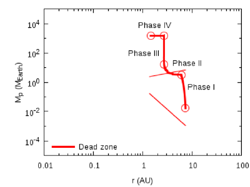
Figure 3.— An evolutionary track of a planet that grows in a dead zone trap. The track (denoted by the thick line) can be divided into four phases. In Phase I, core formation takes place very rapidly in $\tau\sim 10^{5}-10^{6}$ years, which is much faster than the radial movement of the trap at that time. This results in largely vertical motion in the diagram. In Phase II, the core accretes gas onto its envelope. Its timescale is very slow ($\sim 2\times 10^{6}$ years in this case). Therefore, it moves horizontally in this diagram. The mass of the core in Phase I and most of Phase II is within the trapping regime that is represented by the upper and lower thin lines. Toward the end of Phase II, the core drops-out from the trap by opening up a gap in the disk and undergoing type II migration. Phase III is runaway gas accretion onto the core. The timescale of this phase is very short ($<10^{5}$ years). As a result, it moves vertically in this diagram. Planet formation completes during Phase I to III. In Phase IV ($\gtrsim 10^{6}$ years), the gas giant moves inward due to type II migration that is slowed down by the inertia of the planet. When photoevaporation of the gas disk becomes important, type II migration is terminated and its final radial position and orbital period are obtained.

7.2. Planetary growth in all the three planet traps

Fig. 4 shows the computed evolutionary tracks of planets that grow at all three disk inhomogeneities. Different lines at each planet trap correspond to different evolutionary tracks in which planetary growth starts at different times (see Table 5). Despite the difference in the starting time (and position), most planets formed at the dead zone and heat transition traps end up at $r\sim 1$ AU ($\sim 500$ days) and $r\sim 0.1$ AU ($\sim 10$ days), respectively. At the heat transition trap, the surface density of dust is low. Therefore, cores that grow there spend a long time in the trapping phases (Phase I and II). This maximizes the distance over which cores are transported and results in the distribution of cores that hover preferentially around $\gtrsim 1$ AU. Since the low mass cores get distributed over smaller orbital radii and less time remains for the cores to grow up to gas giants, they finally remain less massive ($\lesssim 100M_{\oplus}$), and are located around smaller orbital radii ($\sim 0.1$ AU). The same argument is applied to planets formed in the dead zone trap. However, the surface density of dust at the dead zone is considerably higher than that at the heat transition. Consequently, the final mass of cores trapped at dead zones becomes larger, core formation completes earlier, and the distribution of cores is shifted to $\sim 3$ AU. These combined differences result in the populations of more massive planets orbiting at $\sim 1$ AU.

The evolutionary tracks associated with protoplanets carried by the ice line trap show some differences. The resultant planetary population spreads out over a wider range in the mass-semi-major axis diagram (see Fig. 4). Nonetheless, this can be also understood by the the surface density of dust and the resultant core formation there. At the ice line, the surface densities are substantially higher than that at the dead zone and heat transition and hence the formation of cores is most efficient. This typically results in most massive cores. At the early stage of disk evolution, therefore, the most massive cores are preferentially formed there. They can readily drop-out from the moving trap and pile up around larger orbital radii ($r\sim 5$ AU). These massive cores at larger orbital radii lead to the formation of more massive gas giants that finally orbit at $\gtrsim 1$ AU. In the later stage of disk evolution, the high dust densities at the ice line can still form cores while at that time the other traps not due to lower dust density there. This is the physical reason of the wide spread of planetary population due to the ice line traps.

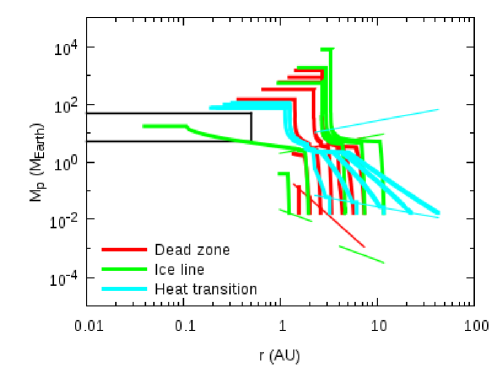
Figure 4.— Evolutionary tracks of planets that grow in all three planet traps. The tracks for the dead zone are denoted by the red thick lines, the ice line by the green, and the heat transition by the light-blue. Corresponding thin lines represent the trapping regimes. Different tracks correspond to planetary growth that initiates at different times (see Table 5). The transport mechanism of cores by planet traps plays the crucial role in producing the mass-period relation; low mass cores that need longer time to grow are more likely to be transported toward smaller orbital radii while massive cores that can readily drop out of the moving traps tend to distribute further away from the star. Thus, there are distinct populations that arise from the difference in the properties of the planet traps and the resultant planetary growth, which results in the trend that planetary mass increases with period. Earlier papers, Ida & Lin (2004, 2008b) predicted a planet desert demarcated by the black rectangle. We emphasize that our model predicts the presence of planets there.

7.3. Comparisons with the observations

We now compare our results with the observations. As already presented in Fig. 4, our model shows that the superposition of all tracks for planets that grow in three planet traps constitutes a theoretical mass-period relation, wherein the final distribution of the mass of the planets is an increasing function of their periods. This is consistent with the observed mass-period relation, as the observational data scatter around the locus of end points of our tracks (see Fig. 5).

This is one of the most important findings in this paper. As discussed in $\S$ 7.2, this arises from the fact that there are considerable differences in the properties of the planet traps that regulate planet formation and migration. As a result, different planet traps have different preferred loci at which evolutionary tracks end up in the mass-semi-major axis diagram. Thus, planet traps act as a filter for distributing cores - massive cores readily drop out from moving traps and tend to orbit further away from the central star while low-mass cores are trapped for a long time and tend to orbit close to the host star - and play the central role in generating the theoretical mass-period relation.

In addition, the prediction that distinct sub-populations can arise depending on the trapping mechanism has several observational consequences. For example, our model provides a physical explanation for the observed pile up of gas giants at $\sim 1$ AU. This again relies on the argument that planet formation efficiency highly depends on the surface density of dust at planet traps. At the dead zone and ice lines, the dust density is expected to be high due to the low disk turbulence, and hence planet formation rates are high there. On the other hand, the formation rate would be low at the heat transition trap due to low dust density. This results in a general trend that more planets are readily formed at the dead zone and ice line traps that end up at $r\sim 1$ AU (see Fig. 5).

Furthermore, our model predicts the population of low mass planets ($\lesssim 50M_{\oplus}$) with $r\lesssim 0.5$ AU. This arises from planet formation that takes place in the moving ice line trap (see Fig. 5). Even in the later stage of disk evolution, the highest dust density there enables the formation of low-mass planets that end up in the desert. On the contrary, the most advanced population synthesis models predict a planet desert there (Ida & Lin 2004, 2008b, also see the footnote 3 in $\S$ 1). The presence of the many observed exoplanets in the region agrees well with our findings.

Finally, our models predict the existence of planet deserts that are quite different in the mass-period space than those claimed by Ida & Lin (2004, 2008b). Fig. 6 shows our deserts, denoted by hatched regions. They are produced due to trapping and subsequent transport of cores. This leads to the evacuation of the cores from these regions in which they have initially grown up. As a result, these regions are regarded as void of planets. More specifically, we define our deserts by estimating the mass ranges of planets that can be captured at the planet traps and following their movement: $M_{p}<M_{gap}$ and $\tau_{mig,I}<\tau_{vis}$ (see $\S$ 5). This kind of planet desert is active only for gas disks. There are a number of possibilities to fill out our deserts: that successive formation of rocky planets after gas disks disperse may ultimately fill out the regime; that, even in the epoch of gas disks, planetary cores formed far beyond our deserts may eventually distribute there due to planetary migration; and that planet-planet scatterings induced by convergence of multiple planet traps may deliver the scattered cores into our deserts. Nonetheless, our predictions are valuable in a sense that such regions are the primary target of the current and ongoing observational surveys (Mayor et al. 2011; Howard et al. 2012).

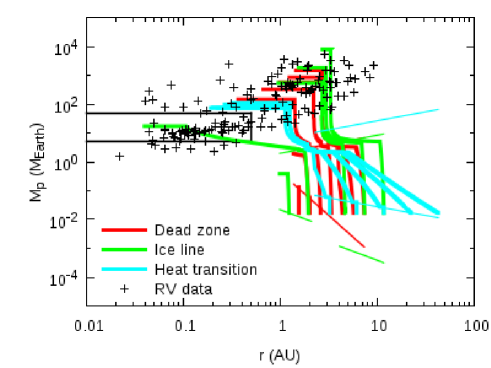
Figure 5.— Comparisons with the observations. The observational data are adopted from Mayor et al. (2011) (as Fig. 1). Our theoretical mass-period relation is consistent with the observations. Also, the presence of many observed low mass planets ($\lesssim 50M_{\oplus}$) at $r\lesssim 0.5$ AU provides further support on our model.

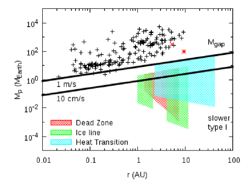
Figure 6.— Prediction of planet deserts for the CTTS case. The desert produced by the dead zone trap is denoted by the red hatched region, the ice line trap by the green, and the heat transition by the light-blue. These regions are the consequence of trapping of type I migrators and defined by the gap opening mass $M_{gap}$ (see equation (28)) and the mass of planets above which they can keep up with the movement of their planet traps (see equation (27), also see Table 3).

8. Parameter studies

We perform parameter studies by varying disk and stellar parameters in order to examine how robust our findings discussed in $\S$ 7.3 are. Also, we investigate the effects of the inertia of planets by changing the value of $f_{mig,slowerII}$ in $\S$ 8.3 to differentiate them from the role of planet traps discussed above.

8.1. Disk parameters

We first focus on parameters for dead zones. We have adopted the parameterized treatment for the structures of dead zones, wherein they are represented by $\Sigma_{A0}$ and $s_{A}$ (see equation (3)). Even in the most recent studies, it is still somewhat uncertain what the precise structure of the dead zones is (Matsumura & Pudritz 2006; Martin et al. 2012). Therefore, we utilize our parameter study in order to discuss how sensitive our findings are to the structures of the dead zones.

Table 6 summarizes parameters we varied. For Runs A1 and A2, the value of $\Sigma_{A0}$ is changed while $s_{A}$ varies for Runs A3 and A4. Any other parameters remain the same as the fiducial ones for all the four runs. Fig. 7 shows the results of the evolution of the positions of three disk inhomogeneities (the left column), the evolutionary tracks of planets (the central column), and the trapping regimes (the right column). The top panels are for the case of Run A1, the second for the Run A2, the third for Run 3, and the bottom for Run4. One immediately observes that the results for all the four cases, especially the behaviors of the evolutionary tracks, are surprisingly similar to those of the fiducial case and give all three key results. Thus, we can conclude that our findings discussed in $\S$ 7.3, are robust even if the structures of dead zones somewhat change due to their surrounding environments and disk configurations.

Table 6Parameter study of dead zones

	$\Sigma_{A0}$ (g cm-2)	$s_{A}$
Run A1	2	3
Run A2	200	3
Run A3	20	1.5
Run A4	20	6

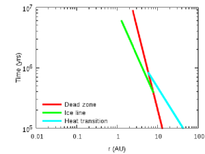
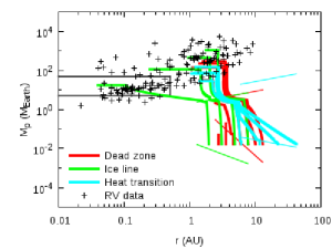
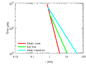
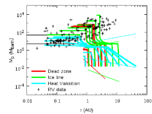
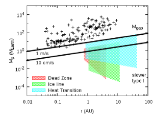
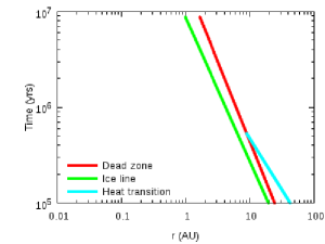
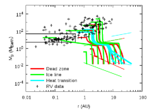
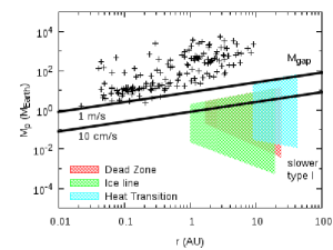
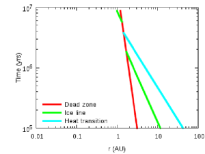
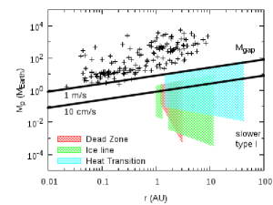
Figure 7.— Parameter study of dead zones (see Table 6). The movements of three planet traps are shown in the left column (as Fig. 2), the evolutionary tracks of planets that grow there in the central (as Fig. 5), and the behaviors of the trapping regimes in the right (as Fig. 6). The top panels show the results of Run A1, the second for Run A2, the third for Run A3, and the bottom for Run A4. The results are quite similar to those of the fiducial model, and hence our important findings such as origins of the observed mass-period relation and the pile up at 1 AU and a prediction of low-mass planets with tight orbits are maintained for dead zones that can have a variety of structures.

8.2. Effects of Stellar mass

The above parameter study leads to the conclusion that disk inhomogeneities and the resultant multiple planet traps play the crucial role in reproducing the key properties of observed exoplanets. Nonetheless, there are few populations of planets that are not covered by the fiducial model: gas giants orbiting at $r\gtrsim 5$ AU. We now examine whether or not this population is also predicted by our model. In order to proceed, we change the stellar mass from 0.5 to $0.9M_{\odot}$ and keep other parameters the same as the fiducial ones. The main motivation for changing the stellar mass is that the observational data are obtained from low- to high-mass stars that cover F, G, and K stars.

Fig. 8 shows the results of the movement of the disk inhomogeneities, the evolutionary tracks of planets that are formed in the traps, and the locations of the planet deserts. This figure confirms that the planets not covered in our previous setup ($10^{2}M_{\oplus}\lesssim M_{p}\lesssim 5\times 10^{3}M_{\oplus}$ and 5 AU $\lesssim r\lesssim$ 10 AU) can indeed be reproduced. This is because high-mass stars result in high accretion rates (see equation (19)), which corresponds to the situation that disks have high mass. As a result, planet formation efficiencies at all three planet traps become high, and most formed planets readily attain high mass, which ends up with planets distributing further away from the central star. Thus, this finding indicates that the full range of the statistical properties of exoplanets can be understood by our model.

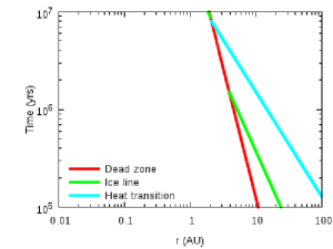
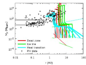
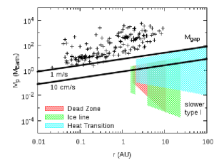
Figure 8.— Parameter study of the variation of stellar mass. The movements of three planet traps are shown in the left panel, the evolutionary tracks of planets that grow there in the central, and the behaviors of the trapping regimes in the right (as Fig. 7). The stellar mass is set as $0.9M_{\odot}$, otherwise the values of the fiducial model are taken. The population of gas giants ($r\gtrsim 5$ AU) not covered by the fiducial model, wherein the stellar mass is 0.5 $M_{\odot}$, is now reproduced. This suggests that the full extent of the data is explained by our model with a modest range of stellar masses, which is part of the data.

8.3. Role of slower type II migration

Based on the above discussion, a number of the fundamental statistical properties of observed exoplanets are most likely to be explained by multiple planet traps that capture and transport planetary cores, depending on planetary mass. As shown in Fig. 4, however, slower type II migration also drives radial drifts in the mass-semi-major axis diagram, following evolutionary tracks of growing planets. In addition, the slower type II migration is a function of planetary mass (see equation (32)). Thus, they imply that a combination of planet traps and slower type II migration (not only planet traps) may play a central role in reproducing the observations. In order to examine the effects of the slower type II migration on our results, we carry out a parameter study in which the value of $f_{mig,slowerII}$ changes (see Table 7).

Fig. 9 shows the results of the evolutionary tracks of planets growing in all the three planet traps. The top left panel shows the results of Run B1, the top right for Run B2, the bottom left for Run B3, and the bottom right for Run B4. For two top panels, there is no mass dependency in equation (32) while it depends on planetary mass for two bottom panels. Comparison of Run B1 (Top left) with any other runs demonstrates that some kind of process which slows down the standard type II migration is clearly needed for reproducing the observed population of exoplanets even if planetary cores are saved due to planet traps. This is because the standard type II migration that proceeds as local viscous timescale leads planets to spiraling into the host stars within the disk lifetime at $r\lesssim$ 10 AU.

When the type II migration somewhat slows down sufficiently, our findings discussed above, especially the mass-period relation, are valid for various cases (see Top right and two Bottom panels). It is important that the overall feature of the resultant populations is very insensitive to the origins of slowing down mechanisms (mass dependence vs independence, compare top right panel with Fig. 5), although the radial distribution somewhat varies for each case. We confirmed, through experiments, that the observed planetary population can be reproduced when $f_{mig,slowerII}\gtrsim 1$ or $f_{mig,slowerII}=\bar{f}M_{crit}/M_{p}$ with $\bar{f}\gtrsim 1$.

In addition to the slower type II migration, photoevaporation of gas is also important for establishing the final radial distribution of planets, since it terminates the migration. The combined effects of type II migration and photoevaporation on planetary populations were discussed in the literature (e.g. Armitage et al. 2002; Matsuyama et al. 2003; Armitage 2007; Alexander & Armitage 2009; Alexander & Pascucci 2012). Our models are more fundamental than theirs in a sense that we have incorporated the effects of type I migration which can be captured at planet traps. We will investigate in detail the combined effects in the forthcoming paper.

In summary, we can conclude that planet traps, not slower type II migration, play the primary role in reproducing the observations, provided that the standard type II migration slows down sufficiently when planetary mass exceeds the local disk mass.

Table 7Parameter study of slower type II migration

	$f_{mig,slowerII}$
Run B1	0
Run B2	1 $\times M_{crit}/M_{p}$
Run B3	0.1
Run B4	10

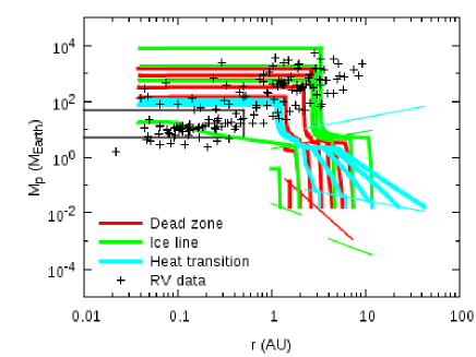
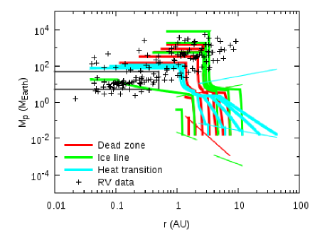
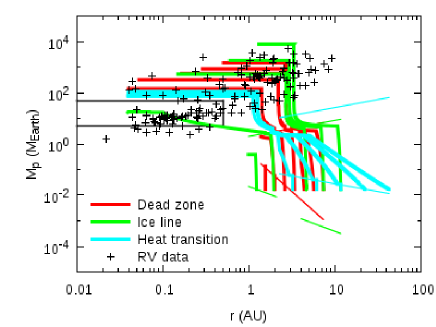
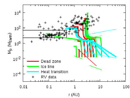
Figure 9.— Parameter study of the effects of slower type II migration (see Table 7). The resultant evolutionary tracks of planets that grow in all the three planet traps are shown (as Fig. 5). The top left panel denotes the results of Run B1, the top right for Run B2, the bottom left for Run B3, and the bottom right for Run B4. For two top panels, the slowing rate is independent of planetary mass while it depends for two bottom panels. When no slowing mechanism is in action (Run B1, $f_{mig,slowerII}=0$), the observed population of exoplanets cannot be reproduced even if planetary cores are captured and distribute by moving planet traps. The observations can be reproduced only if the standard type II migration sufficiently slows down ($f_{mig,slowerII}\gtrsim 1$ or $f_{mig,slowerII}=\bar{f}M_{crit}/M_{p}$ with $\bar{f}\gtrsim 1$). It is important that mass dependency on the slowing mechanism of the type II migration does not matter. Thus, this suggests that planet traps are more crucial for understanding the statistics of observed exoplanets.

9. Discussion & Conclusions

We have constructed and followed the evolutionary tracks of protoplanets generated by combining core accretion together with the movement of planet traps in evolving disks. We have focused on three types of inhomogeneities in protoplanetary disks and the resultant planet traps: dead zones, ice lines, and heat transitions.

We have demonstrated that the plant traps play two fundamental roles in planet formation and migration. The first is to trap cores of gas giants that otherwise undergo rapid type I migration. This trapping leads to the formation of gas giants orbiting at 0.01 AU $\lesssim r\lesssim$ 10 AU without the cores falling into the central star before disk evolution is terminated by disk photoevaporation. The second is to transport the trapped cores very slowly from large to small periods. This transport distance is regulated by the gap opening mass and the properties of the planet traps and hence is well coupled with planetary growth histories; different planet traps result in different efficiencies of planet formation and migration. Consequently, planet traps are regarded effectively as a filter for distributing cores - massive cores tend to hover around large periods while low-mass cores around short periods.

We have seen that the combination of planet traps, planetary growth and type II migration in evolving disks generates planetary populations that have a wide range in mass and period. The final positions of planets are determined when photoevaporation of gas disks (rather than disk viscosity) plays the dominant role in disk evolution. It is noted that the final distribution of planets can be largely affected by the combination of slower type II migration and the photoevaporation rate that is adjusted by $f_{pe}$ (see equation (20) and Table 2). In order to examine this dependency, we will perform a more comprehensive parameter study in a subsequent paper. In addition, different accretion histories of planets will result in differences in the composition of the planets and their atmospheres, which can be investigated by extending our models.

What about purely dynamical effects arising from planet-planet interactions? These are well known to be important for understanding the observed eccentricity distribution (e.g. Rasio & Ford 1996). However, Matsumura et al. (2010) have recently clarified through numerical simulations that the semi-major axes of planets are determined mainly by planetary migration in the gas disks while the eccentricities are determined after the gas disks dissipate severely. This indicates that the results of planetary evolution in the gas disk phase will not be washed out by subsequent planetary dynamics.

We list our major findings below.

1. We have demonstrated that the wide range of end points of planets evolving in the mass-semi-major axis diagram establishes a theoretical mass-period relation in which planetary mass is an increasing function of orbital period (see Fig. 5). This is in excellent agreement with the observational data in a sense that the data scatter around the end point of our evolutionary tracks.

2. We have shown that the many tracks of dead zones and ice lines preferentially tend to end up at $\sim$ 1 AU (see Fig. 5). Combined with an argument that planet formation efficiencies are reasonably high there, the preference provide a physical explanation for the pile up of observed gas giants at $\sim$ 1 AU.

3. We have also demonstrated that planets that grow in dead zone traps end up at $r\sim$ 1 AU, ice line traps at 0.03AU $\lesssim r\lesssim$ 3 AU, and heat transition traps at $r\sim$ 0.1 AU (see Fig. 4). The resulting wide range of planets in the mass-semi-major axis diagram is insensitive to the detailed structure of dead zones and accounts for a number of important observational trends.

4. We have also shown that moving ice line traps can put planets in the planet deserts that were predicted by the earlier population synthesis models (see Fig. 5). As denoted by Fig. 1, the desert is located in the range of planetary masses (5-50 $M_{\oplus}$) and semi-major axes (0.04-0.5 AU). The recent observations discover many planets in the deserts. Thus, our models are more consistent with the observations in this regard.

5. We predict planet deserts that arise from the nature of planet traps. They have physically different origins from the earlier claimed ones. Our deserts are relevant only when protoplanetary disks have sufficient amount of gas that drives rapid type I migration. This suggests that the deserts can be filled by planets that form far beyond the deserts and eventually migrate there in gas disks. The planets are likely to emerge after the gas disks severely disperse and/or to be transported there due to planet-planet scatterings. Our deserts are present in the range of planetary masses (1-50 $M_{\oplus}$) and semi-major axes (1-10 AU), which covers the primary target of ongoing and future observational surveys such as the HARPS and Kepler missions.

6. The more massive the host star, the more the evolutionary tracks in the mass-period diagram are pushed towards large disk radii. This arises because of the much more rapid accretion rates in more massive systems ($\dot{M}\propto M_{*}^{2}$).

In the forthcoming paper, we will use N-body simulations to take into account the physics of planet-planet interactions that can be induced by growing planets in different planet traps.

Appendix A A: Characteristic masses in the mass-semi-major axis diagram

We discuss the segmentation of a diagram for planetary mass versa semi-major axis. As an example,the bottom panel of Fig. 10 (Left) shows evolution of four characteristic masses ($M_{max}$, $M_{crit}$, $M_{gap}$, and $M_{mig,I}$) at a dead zone for the fiducial case (also see Table 3). Every position of the dead zone that is specified by the time $\tau$ defines four masses (see circles on Fig. 10 (Left) as an example). As the dead zone moves inwards following the disk evolution (see the top panel of Fig. 10 (Left)), these four masses also move inwards at the same rate. As a result, four lines are drawn that track the evolution of the characteristic masses in the diagram. The top line denotes $M_{max}$, the second for $M_{crit}$, the third for $M_{gap}$, and the bottom for $M_{mig,I}$. Thus, the top and third lines define the boundaries of type II migration in the mass-semi major axis diagram while the third and bottom one defines the boundaries for trapping type I migration. The second line defines where the inertia of planetary mass becomes effective that can slow down type II migration.

The bottom panel of Fig. 10 (Right) shows the evolution of four characteristic masses at all three disk inhomogeneities for the fiducial case. The type II regimes for each inhomogeneity are denoted by the coarse hatch regions while the fine hatch ones represent the type I trap regimes. The solid lines denote $M_{crit}$. The dead zone is denoted by red, the ice line by green, and the heat transition by light blue. Disappearance and re-appearance of these regions correspond to the behavior of each inhomogeneity that is shown in the top panel.

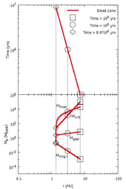
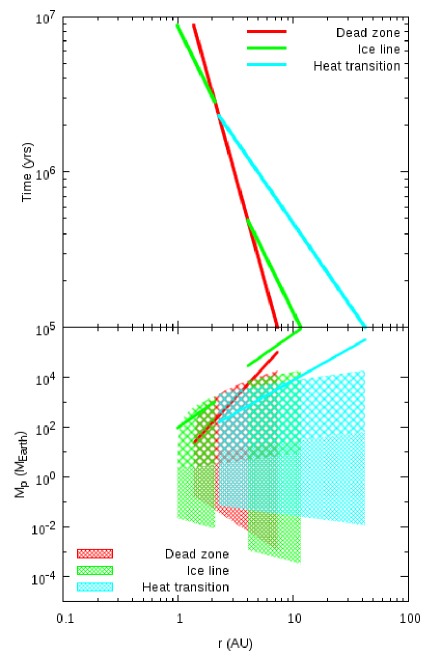
Figure 10.— Left: (Top) The movement of a dead zone trap in evolving disks. The initial position is determined by assuming a start time of $10^{5}$ years. The final position arises when the accretion rate $\dot{M}$ equals the photoevaporation rate $\dot{M}_{pe}$, - a condition which also defines the disk lifetime ($\tau_{disk}\simeq 8.8\times 10^{6}$ years in our fiducial model). (Bottom) The evolution of four characteristic masses at the dead zone trap. The top line represents $M_{max}$, the second for $M_{crit}$, the third for $M_{gap}$, and the lowest one for $M_{mig,I}$ (see Table 3). Every position of the dead zone (shown in the top panel) defines four masses (see some symbols as examples), and as the dead zone moves inward, they also move inward. Right: (Top) The movement of all three traps in evolving disks. The dead zone trap is denoted by red, the ice line by green, and the heat transition by light blue. They move inward due to viscous evolution of the disks, but at different rates. (Bottom) The evolution of four characteristic masses at all three traps. The color scheme is the same as the top panel. The type II regimes that are defined by $M_{max}$ and $M_{gap}$, are denoted by the coarse hatched regions while the trapping regimes that are specified by $M_{gap}$ and $M_{mig,I}$ are represented by the fine hatched regions. The solid lines denote $M_{crit}$. The disappearance and re-emergence of these regimes correspond to those of the positions of the planet traps that are shown in the top panel.

Appendix B B: Analytical prescriptions for planetary growth

We summarize the standard results of the core accretion scenario needed to follow the growth of planets as they move in disks.

B.1. Stage I: Formation of cores

Formation of cores in planetesimal disks is well understood in the literature (e.g. Kokubo & Ida 2002), and the growth timescale in the disks is given as

$$\tau_{c,acc} \simeq 1.2\times 10^{5}\mbox{ yr}\left(\frac{\Sigma_{d}}{10\mbox{ g cm}^{-2}}\right)^{-1}\left(\frac{r}{r_{0}}\right)^{1/2}\left(\frac{M_{c}}{M_{\oplus}}\right)^{1/3}\left(\frac{M_{*}}{M_{\odot}}\right)^{-1/6}$$

$$\times \left[\left(\frac{b}{10}\right)^{-1/5}\left(\frac{\Sigma_{g}}{2.4\times 10^{3}\mbox{ g cm}^{-3}}\right)^{-1/5}\left(\frac{r}{r_{0}}\right)^{1/20}\left(\frac{m}{10^{18}\mbox{ g}}\right)^{1/15}\right]^{2},$$

where $\Sigma_{d}$ is the surface density of dust, $M_{c}$ is the mass of a core, $b=10$ is a parameter for determining the feeding zone of the core (see below), and $m=10^{18}$g is the mass of planetesimals that are accreted onto the core. Adopting this timescale, the growth of cores is regulated by

$$\frac{dM_{p}}{dt}=\frac{M_{p}}{\tau_{c,acc}}.$$ (B2)

B.2. Stage II: slow gas accretion onto the envelopes

As cores grow, their feeding zones $\triangle r_{c}$ empty. These zones are scaled by $br_{H}$, where $r_{H}=(M_{c}/(3M_{*}))^{1/3}$ is the Hill radius of a core and $b\sim 10$. The decrease of planetesimals in the zones results in the reduction of the accretion rate of cores $\dot{M}_{c}$. In the limit of the modest to high velocity dispersion $\sigma$ of planetesimals that are accreted onto the cores, $\dot{M}_{c}$ can be written as (Safronov 1972; Ida & Lin 2004)

$$\dot{M}_{c}\sim 2\pi\left(\frac{R_{c}}{r}\right)\left(\frac{M_{c}}{M_{*}}\right)\left(\frac{r\Omega}{\sigma}\right)^{2}\Sigma_{d}r^{2}\Omega,$$ (B3)

where $R_{c}$ is the radius of cores. Planetesimals within the feeding zones can reach cores when $\sigma/\Omega\sim\triangle r_{c}(=br_{H})$. Assuming $R_{c}$ to be similar to that of the Earth;

$$R_{c}=6.4\times 10^{8}\mbox{ cm}\left(\frac{M_{c}}{M_{\oplus}}\right)^{1/3}\left(\frac{\rho_{c}}{5.5\mbox{ g cm}^{-3}}\right)^{-1/3},$$ (B4)

$\dot{M}_{c}$ is given as

$$\dot{M}_{c}\sim 3.0\times 10^{-8}M_{\oplus}\mbox{ yr}^{-1}\left(\frac{b}{10}\right)^{-2}\left(\frac{\rho_{c}}{5.5\mbox{ g cm}^{-3}}\right)^{-1/3}\left(\frac{M_{c}}{M_{\oplus}}\right)^{2/3}\left(\frac{M_{*}}{M_{\odot}}\right)^{-1/3}\left(\frac{\Sigma_{d}}{10\mbox{ g cm}^{-2}}\right)\left(\frac{r}{r_{0}}\right)\left(\frac{\mbox{ yr}}{1/\Omega}\right).$$ (B5)

When all the planetesimals in their feeding zones are consumed, the cores attain the maximum mass that is known as the isolation mass, which is defined by (Kokubo & Ida 2002; Ida & Lin 2004)

$$M_{c,iso}=2\pi r\vartriangle r_{c}\Sigma_{d}\simeq 0.16M_{\oplus}\left(\frac{b}{10}\right)^{3/2}\left(\frac{\Sigma_{d}}{10\mbox{ g cm}^{-2}}\right)^{3/2}\left(\frac{r}{r_{0}}\right)^{3}\left(\frac{M_{*}}{M_{\odot}}\right)^{-1/2}.$$ (B6)

The accretion of gas onto cores and subsequent envelope formation are initiated when the mass of core becomes larger than

$$M_{c,crit}\simeq 10f_{c,crit}M_{\oplus}\left(\frac{\dot{M}_{c}}{10^{-6}M_{\oplus}\mbox{ yr}^{-1}}\right)^{1/4}.$$ (B7)

This critical mass was originally derived from a series of numerical simulations that investigated the effect of cores’ accretion rates and opacity in the envelope on formation of gas giants (Ikoma et al. 2000). Here, we have adopted a simplified one, following Ida & Lin (2004). Recent studies, however, revealed that $M_{c,crit}$ might be smaller than that predicted by equation (B7) with $f_{c,crit}=1$ (e.g. Hori & Ikoma 2011). In order to take this into account, we have introduced a dimensionless factor $f_{c,crit}$.

The gas accretion rate of cores is prescribed by (Ida & Lin 2004)

$$\frac{dM_{p}}{dt}\simeq\frac{M_{p}}{\tau_{KH}},$$ (B8)

where the Kelvin-Helmholtz timescale is given as

$$\tau_{KH}\simeq 10^{c}\mbox{ yr}\left(\frac{M_{p}}{M_{\oplus}}\right)^{-d},$$ (B9)

where $c=8$ and $d=2.5$. This is a simplified timescale that was originally estimated from numerical simulations (Ikoma et al. 2000). As shown by the more detailed numerical simulations (Pollack et al. 1996; Lissauer et al. 2009), this stage is slow ($\gtrsim 10^{6}$ years).

B.3. Stage III: runaway gas accretion onto the cores

When planets become massive enough, runaway gas accretion onto the cores starts. In the detailed numerical simulations, this stage commences when the envelope of cores becomes more massive than the cores (Pollack et al. 1996; Ikoma et al. 2000; Lissauer et al. 2009). Nonetheless, we monitor this stage by the condition that

$$\frac{\tau_{KH}}{10^{5}\mbox{ yr}}<1.$$ (B10)

This is because our approach is rather simple. This condition never affects our results. The growth rate of this stage is also prescribed by equation (B8).

It is totally unclear how gas accretion onto the cores terminates and what physical process(es) determines the final mass of gas giants. Therefore, we assume that Stage III continues until planets gain the mass $f_{max}M_{max}$, where $f_{max}$ is an adjustable parameter.

B.4. Parameters for planetary growth

As discussed above, planetary growth and consequent evolutionary tracks of planets are regulated by four parameters in our model (see Table 8). The parameter $f_{c,crit}$ governs the onset of gas accretion of cores, a set of parameters $c$ and $d$ determine the efficiency of gas accretion onto cores, and $f_{max}$ controls the final mass of planets. We denote these values given in Table 8 our fiducial model. Note that Ida & Lin (2004) adopted the values of $f_{c,crit}=1$, $c=9$, and $d=3$ rather than our set of $f_{c,crit}=0.3$, $c=8$, and $d=2.5$. We performed a parameter study and confirmed that different choice of these values does not change our results very much. Therefore, our choice and results are robust in a sense that we can compare our results with the results of Ida & Lin (2004, 2008b). We present only a parameter study of $f_{max}$ in Appendix C, because the choice of this value is probably the most uncertain.

Table 8Important parameters for planetary growth

Symbols	Meaning	Value
$f_{c,crit}$	A factor linked to the critical mass of cores (equation (B7))	0.3
$c$	Exponent of the Kelvin-Helmholtz timescale (equation (B9))	8
$d$	Exponent of the Kelvin-Helmholtz timescale (equation (B9))	2.5
$f_{max}$	A factor linked to the maximum mass of planets	0.1

Appendix C C: A parameter study for planet growth

As discussed in Appendix B, our choice of most parameters that regulate planetary growth is based on the physical considerations and the more recent results of detailed simulations. Hence our choice is compatible with the original work of (Ida & Lin 2004). However, there is one exception, which is $f_{max}$ which constrains the maximum mass of planets. This is mainly because there are no firm physical arguments and simulations of how the final mass of planets is established. Therefore, we now examine how the value of $f_{max}$ affects our results.

Table 9 summarizes our parameter study on $f_{max}$. For Run C1, we took $f_{max}=0.03$ while $f_{max}=0.3$ for Run C2. Except for the value of $f_{max}$, we adopted the same values of the fiducial model. Fig. 11 shows the results of the evolutionary tracks of planets for both cases. The left panel shows the results of Run C1 while the right one for the Run C2. The results of both cases are generally very similar to that of the fiducial model. More specifically, both cases produced theoretical mass-period relations that are broadly consistent with the observations. On closer examination, we see that the pile up of gas giants at $\sim 1$ AU and the presence of low-mass planets with small orbital radii are relatively affected by the value of $f_{max}$. This is indeed expected. If $f_{max}$ has a small value, then low mass planets become the main product and planet formation completes earlier. Consequently, the planets experience substantial inward type II migration. In addition, the effect of the inertia of the planets that slows down the type II migration is also reduced. This results in larger populations of low-mass planets at small orbital radii. Thus, models with small values of $f_{max}$ have difficulty in reproducing the pile up at 1 AU. The opposite happens for large values of $f_{max}$. In this case, massive planets are preferentially formed and the completion of planet formation takes place at later time, so that the subsequent inward type II migration is significantly suppressed due to both the shorter remaining time and the larger inertia of planets. As a result, the population of low-mass planets with tight orbits declines while the 1 AU pile up is enhanced.

In summary, the results depend slightly on some basic parameters such as $f_{max}$. Nonetheless, they are well understood by the physical arguments presented in $\S$ 7. Therefore, our findings are reasonably robust for a wide range of the parameter space.

Table 9Parameter study of planetary growth

	$f_{max}$
Run C1	0.03
Run C2	0.3

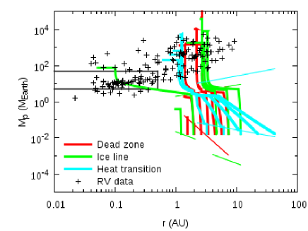
Figure 11.— Parameter study of the variation of maximum mass of planets $f_{max}$ (see Table 9). The evolutionary tracks of planets that grow in all three planet traps are shown (as Fig. 5). The result of Run C1 ($f_{max}=0.03$; low mass case) is presented in the left panel while that of Run C2 ($f_{max}=0.3$; high mass case) in the right. Although the pile up at 1 AU and low mass planets with small orbital radii are slightly affected by $f_{max}$, the resultant populations are still well understood by the physical considerations discussed in $\S$ 7.

References

- Adams et al. (2004) Adams, F. C., Hollenbach, D., Laughlin, G., & Gorti, U. 2004, ApJ, 611, 360
- Alexander & Armitage (2009) Alexander, R. D. & Armitage, P. J. 2009, ApJ, 704, 989
- Alexander & Pascucci (2012) Alexander, R. D. & Pascucci, I. 2012, MNRAS, 422, L82
- Armitage (2007) Armitage, P. J. 2007, ApJ, 665, 1381
- Armitage (2011) —. 2011, ARA&A, 49, 195
- Armitage et al. (2002) Armitage, P. J., Livio, M., Lubow, S. H., & Pringle, J. E. 2002, MNRAS, 334, 248
- Balbus (2003) Balbus, S. A. 2003, ARA&A, 41, 555
- Calvet et al. (2004) Calvet, N., Muzerolle, J., sar Briceño, C., Hernández, J., Hartmann, L., Saucedo, J., & Gordon, K. D. 2004, AJ, 128, 1294
- Chiang & Goldreich (1997) Chiang, E. I. & Goldreich, P. 1997, ApJ, 490, 368
- D’Alessio et al. (1998) D’Alessio, P., Cantó, J., Calvet, N., & Lizano, S. 1998, ApJ, 500, 411
- Dullemond et al. (2007) Dullemond, C. P., Hollenbach, D., Kamp, I., & D’Alessio, P. 2007, Protostars and Planets V (Tucson: Univ. Arizona Press)
- Gammie (1996) Gammie, C. F. 1996, ApJ, 457, 355
- Gorti et al. (2009) Gorti, U., Dullemond, C. P., & Hollenbach, D. 2009, ApJ, 705, 1237
- Gorti & Hollenbach (2009) Gorti, U. & Hollenbach, D. 2009, ApJ, 690, 1539
- Hartmann et al. (1998) Hartmann, L., Calvet, N., Gullbring, E., & D’Alessio, P. 1998, ApJ, 495, 385
- Hasegawa & Pudritz (2010a) Hasegawa, Y. & Pudritz, R. E. 2010a, ApJ, 710, L167
- Hasegawa & Pudritz (2010b) —. 2010b, MNRAS, 401, 143
- Hasegawa & Pudritz (2011a) —. 2011a, MNRAS, 413, 286
- Hasegawa & Pudritz (2011b) —. 2011b, MNRAS, 417, 1236
- Hellary & Nelson (2012) Hellary, P. & Nelson, R. P. 2012, MNRAS, 419, 2737
- Hollenbach et al. (1994) Hollenbach, D., Johnstone, D., Lizano, S., & Shu, F. 1994, ApJ, 428, 654
- Hori & Ikoma (2011) Hori, Y. & Ikoma, M. 2011, MNRAS, 416, 1419
- Howard et al. (2012) Howard, A. W. et al. 2012, ApJS, 201, 15
- Ida & Lin (2004) Ida, S. & Lin, D. N. C. 2004, ApJ, 604, 388
- Ida & Lin (2008a) —. 2008a, ApJ, 673, 487
- Ida & Lin (2008b) —. 2008b, ApJ, 685, 584
- Ida & Lin (2010) —. 2010, ApJ, 719, 810
- Ikoma et al. (2000) Ikoma, M., Nakazawa, K., & Emori, H. 2000, ApJ, 537, 1013
- Ilgner & Nelson (2006) Ilgner, M. & Nelson, R. P. 2006, A&A, 445, 205
- Ivanov et al. (1999) Ivanov, P. B., Papaloizou, J. C. B., & Polnarev, A. G. 1999, MNRAS, 307, 79
- Jang-Condell & Sasselov (2004) Jang-Condell, H. & Sasselov, D. D. 2004, ApJ, 608, 497
- Johnstone et al. (1998) Johnstone, D., Hollenbach, D., & Bally, J. 1998, ApJ, 499, 758
- Kokubo & Ida (1998) Kokubo, E. & Ida, S. 1998, Icarus, 131, 171
- Kokubo & Ida (2002) —. 2002, ApJ, 581, 666
- Kretke & Lin (2007) Kretke, K. A. & Lin, D. N. C. 2007, ApJ, 664, L55
- Kretke & Lin (2012) —. 2012, ApJ, 755, 74
- Lissauer et al. (2009) Lissauer, J. J., Hubickyj, O., D’Angelo, G., & Bodenheimer, P. 2009, Icarus, 199, 338
- Lynden-Bell & Pringle (1974) Lynden-Bell, D. & Pringle, J. E. 1974, MNRAS, 168, 603
- Lyra et al. (2010) Lyra, W., Paardekooper, S.-J., & Mac Low, M.-M. 2010, ApJ, 715, L68
- Martin et al. (2012) Martin, R. G., Lubow, S. H., Livio, M., & Pringle, J. E. 2012, MNRAS, 420, 3139
- Masset et al. (2006) Masset, F. S., Morbidelli, A., Crida, A., & Ferreira, J. 2006, ApJ, 642, 478
- Matsumura & Pudritz (2006) Matsumura, S. & Pudritz, R. E. 2006, MNRAS, 365, 572
- Matsumura et al. (2007) Matsumura, S., Pudritz, R. E., & Thommes, E. W. 2007, ApJ, 660, 1609
- Matsumura et al. (2009) —. 2009, ApJ, 691, 1764
- Matsumura et al. (2010) Matsumura, S., Thommes, E. W., Chatterjee, S., & Rasio, F. A. 2010, ApJ, 714, 194
- Matsuyama et al. (2003) Matsuyama, I., Johnstone, D., & Murray, N. 2003, ApJ, 585, L143
- Mayor et al. (2011) Mayor, M. et al. 2011, preprint (astro-ph/arXiv:1109.2497v1)
- Menou & Goodman (2004) Menou, K. & Goodman, J. 2004, ApJ, 606, 520
- Min et al. (2011) Min, M., Dullemond, C. P., Kama, M., & Dominik, C. 2011, Icarus, 212, 416
- Mordasini et al. (2009) Mordasini, C., Alibert, Y., & Benz, W. 2009, A&A, 501, 1139
- Muzerolle et al. (2005) Muzerolle, J., Luhman, K. L., sar Briceño, C., Hartmann, L., & Calvet, N. 2005, ApJ, 625, 906
- Owen et al. (2012) Owen, J. E., Clarke, C. J., & Ercolano, B. 2012, MNRAS, 422, 1880
- Owen et al. (2011) Owen, J. E., Ercolano, B., & Clarke, C. J. 2011, MNRAS, 412, 13
- Owen et al. (2010) Owen, J. E., Ercolano, B., Clarke, C. J., & Alexander, R. D. 2010, MNRAS, 401, 1415
- Paardekooper et al. (2010) Paardekooper, S.-J., Baruteau, C., Crida, A., & Kley, W. 2010, MNRAS, 401, 1950
- Pollack et al. (1996) Pollack, J. B., Hubickyj, O., Bodenheimer, P., Lissauer, J. J., Podolak, M., & Greenzweig, Y. 1996, Icarus, 124, 62
- Rasio & Ford (1996) Rasio, F. A. & Ford, E. B. 1996, Science, 274, 954
- Safronov (1972) Safronov, V. S. 1972, Evolution of the Protoplanetary Cloud and Formation of the Earth and Planets (Jerusalem: Israel Program for Scientific Translations)
- Sano et al. (2000) Sano, T., Miyama, S., Umebayashi, T., & Nakano, T. 2000, ApJ, 543, 486
- Shakura & Sunyaev (1973) Shakura, N. I. & Sunyaev, R. A. 1973, A&A, 24, 337
- Syer & Clarke (1995) Syer, D. & Clarke, C. J. 1995, MNRAS, 277, 758
- Tanaka et al. (2002) Tanaka, H., Takeuchi, T., & Ward, W. R. 2002, ApJ, 565, 1257
- Udry & Santos (2007) Udry, S. & Santos, N. C. 2007, ARA&A, 45, 397
- Ward (1997) Ward, W. R. 1997, Icarus, 126, 261
- Wetherill & Stewart (1989) Wetherill, G. W. & Stewart, G. R. 1989, Icarus, 77, 330
- Yamada & Inaba (2012) Yamada, K. & Inaba, S. 2012, MNRAS, 424, 2746