Local Water Diffusion Phenomenon Clustering From High Angular Resolution Diffusion Imaging (HARDI)††thanks: This work is supported by Samuel de Champlain 63.102 funds
Abstract
The understanding of neurodegenerative diseases undoubtedly passes through the study of human brain white matter fiber tracts. To date, diffusion magnetic resonance imaging (dMRI) is the unique technique to obtain information about the neural architecture of the human brain, thus permitting the study of white matter connections and their integrity. However, a remaining challenge of the dMRI community is to better characterize complex fiber crossing configurations, where diffusion tensor imaging (DTI) is limited but high angular resolution diffusion imaging (HARDI) now brings solutions. This paper investigates the development of both identification and classification process of the local water diffusion phenomenon based on HARDI data to automatically detect imaging voxels where there are single and crossing fiber bundle populations. The technique is based on knowledge extraction processes and is validated on a dMRI phantom dataset with ground truth.
1 Introduction
Diffusion Weighted magnetic resonance imaging (DW-MRI) is able to quantify the anisotropic diffusion of water molecules in biological tissues such as the human brain white matter. The great success of DW-MRI comes from its capability to accurately describe the geometry of the underlying microstructure. DW-MRI captures the average diffusion of water molecules, which probes the structure of the biological tissue at scales much smaller than the imaging resolution [3]. New dMRI techniques for high angular resolution diffusion imaging (HARDI) are now able to recover one or more directions of fiber populations at each imaging voxel and thus, overcome some of the limitations of diffusion tensor imaging (DTI) in regions of complex fiber configurations where fibers cross, branch and kiss.
Most current classification techniques are based on DTI measures of Westin et al [12]. For example, a recent paper from [10] classifies the white matter voxels into single and crossing fibers simply by hard thresholding the linear, planar and spherical measures computed from the eigen-values of the diffusion tensor. Other techniques have been developed to better handle fiber crossings using apparent diffusion coefficient [2] modeling from HARDI and other HARDI models representations based on spherical harmonics (SH) decomposition [7]. It was previously suggested using automatic Bayesian relevance determination [1] that between 1/3 and 2/3 of WM voxels contained crossings. Jeurissen et al [6] have just showed that this number is an underestimation and that WM crossings can take up to 90% of WM voxels using maxima extracted from a robust SH-based fiber orientation distribution estimation using constrained spherical deconvolution. Otherwise, the first attempts to classify HARDI voxels using machine learning techniques was done in [11] using the space of SH coefficients from q-ball imaging. These techniques are based on diffusion maps and spectral clustering but were never applied to neurodegenerative datasets. More recently, Schnell et al. [8] have designed a classification process based on support vector machines, also based on the SH representation of the dMRI signal and have compared their results with the classical classification of Westin’s measures, as done in [10].
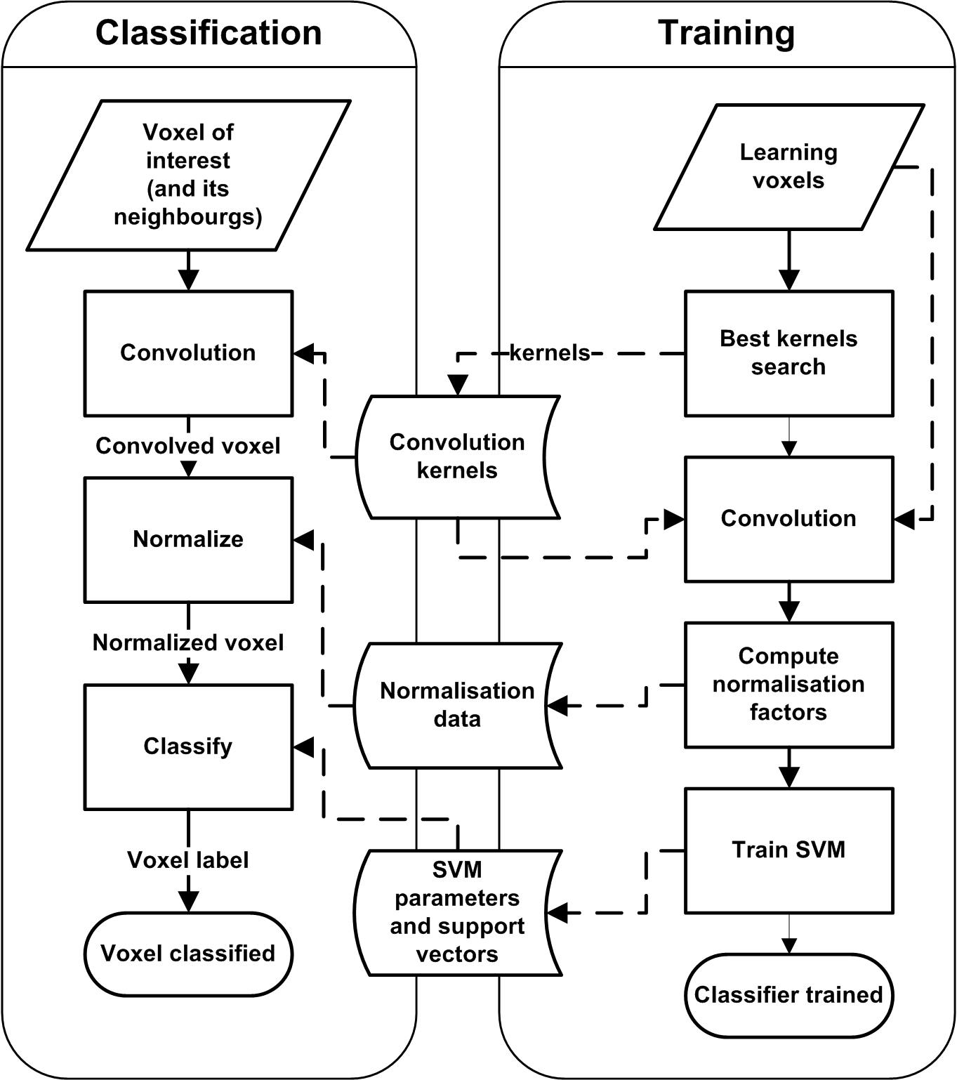
The main contribution of this paper is the creation of a system allowing to automatically classify voxels of HARDI data in order to segment the white matter among different classes. The proposed method goes deeper than the approach presented in [8] because it takes into account the neighbourhood of the voxels by using convolved data.
2 Classifier Creation and Evaluation
2.1 Proposed Approach
Using the Spherical Harmonic (SH) representation of each voxel [2], we want to be able to classify it as: (a) white matter with a single fiber bundle (WMSF), (b) white matter with crossing fiber bundles (WMCF), (c) non-white matter (N-WM) of type gray matter (GM) or cerebrospinal fluid (CSF). Section 3.1 presents the dataset. We use a Support Vector Machine (SVM) [9] classifier to obtain the label of a voxel. The SVM tries to find the best separating hyperplane between two classes. As we work with several classes, a one-against-one approach is used (we train classifiers).
We easily see that using only the SH information may be not enough accurate, as there is no knowledge of the neighborhood while classifying the voxel. To address this problem, we operate a 2D convolution of each slice of the brain against a kernel. This allows to work with a voxel representation resulting of a weighted sum of the neighboring voxels. The convolution kernels are chosen in order to obtain the best accuracy (see Section 2.4).
2.2 Classification of Voxel Using a Particular Feature Space and its Kernels
Say we have the selected feature space of cardinality (i.e., each voxel is represented by a vector of size ; depends on the SH order) and , the convolution kernels with one convolution kernel per dimension of the features space. We apply the convolution kernel on each feature of each voxel of each slice :
| (1) |
with the feature of the voxel located at position of the slice , the slice after convolution of all voxels and features and the number of slices. Now, we consider all the voxels as being in a whole set of couples ( is the feature vector and its label) whatever their slice and localisation in the slice:
| (2) |
with the label of the voxel at () in slice ).
We apply a 6 fold stratified cross validation (we obtain 6 subsets, where each label is represented at the same ratio in each subset: there is the same recognition difficulty in each subset). Each subset serves as a testing set, while the other subsets serve as training set (the following procedure is then applied 6 times). The mean () and the standard deviation () of the feature vectors of the training set is computed in order to apply a zscore normalisation of the training and testing sets (). The normalised training samples serve to train a SVM with a gaussian kernel. To quickly evaluate the couple (, ) we do not try to search the best SVM parameters. So and are at the default value of libsvm (). The learned SVM is used to predict the label of the testing samples.
2.3 Evaluation of a Set Kernels for a Feature Space
There is a large disparity in the number of individuals of each class. So, we do not want to simply compute an averaged classification error rate. Instead we compute the following errors: (i) Missed WM Ratio (MWMR): ratio of WMSF and WMCF voxels recognized as being N-WM (CSF or GM) voxels; (ii) Exchanged WM Ratio (EWMR): ratio of WMSF voxels recognized as being WMCF voxels and WMCF voxels recognized as WMSF voxels; (iii) Imagined WM ratio (IWMR): ratio of N-WM (CSF and GM) voxels recognised as being WMSF or WMCF voxels. Then the final error score is computed as following:
| (3) |
with , and in this experiment. This way, we give a low weight on the EWMR and bigger weights on IWMR and MWMR. Although we try to differenciate them, we do not care of exchanging CSF and GM.
2.4 Selection of the Best Kernels
As, for each feature set, the search space is very huge, we use a genetic algorithm in order to search the best convolution kernels. Each kernel is an array of size , with the width of the kernel. The genome consists of the kernels stored in a 1D array using values in the interval (it means that values inside the kernel will be in this interval), so it has a size of . We do not pay attention to have a kernel summing to as we do not care if the data obtained after convolution is not in the same metric as the original data (we do not manipulate or visualize the convolved data, it only serves for classification). Population contains 500 individuals. The initial population contains:
-
•
one individual build with gaussian kernels which are supposed to be good by doing a weighted average based on the distance around the voxel of interested
-
•
250 individuals created with modification of the first individual (mean of the gaussian kernels based individual and a random one
-
•
249 individuals generated totally randomly.
The procedure stops after 100 generations or 3 days of computing. The cross-over rate is set at 0.9 and use 2 points. The mutation rate is set at 0.1 (a higher mutation did not implyied a faster convergence nor better results) and apply gaussian mutations. The number of elites is set at 20. The fitness value of a chromosome is the explained in (3) and the genetic algorithm wants to reduce this rate.
3 Measure of Performance
3.1 Apparatus
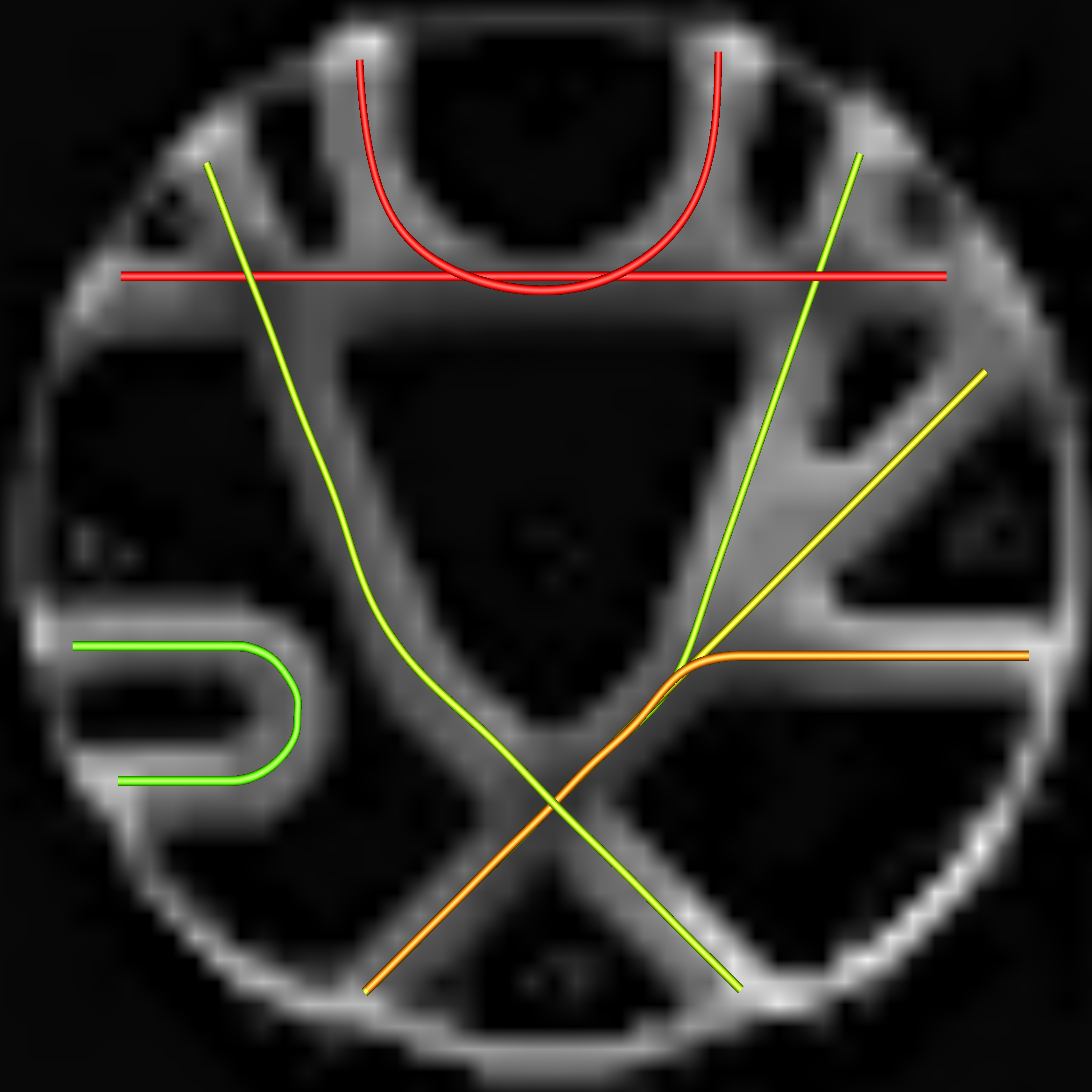
Ground truth datasets and validation is one of the biggest challenge of the dMRI community. Hence, there is an important effort to build ex-vivo phantoms that produce realistic datasets, more realistic than simulated synthetic data. This is the case of the FiberCup data, mimicking a coronal slice of the brain. It is a simple 3D dMRI dataset, but is quite unique because it reproduces complex fiber crossing configurations, similar to configurations in the cemtrum semioval and ’U’ fibers of the brain. The underlying ground truth is known and thus will serve as our learning/testing dataset. For this paper, we have focused on the mm isotropic, 64 directions, s/mm2 dataset [4]. The phantom and ground truth fibers are illustrated in Fig. 2. Thus, we use a good compromise between synthetic data as in [8] and in vivo data for which it almost impossible to have ground truth. Phantom border represents GM, fibers in one direction (resp. several directions) is WMSF (resp. WMCF), the rest is CSF.
From this HARDI dataset, we provide one input among the following choices to the SVM: i)-ii) a SH order 4 and 8 representation of raw signal (SH4, SH8 respectively) [2], or iii) the eigenvalues of the diffusion tensor [12] (EIG).
Results of the proposed method are compared to a baseline classifier. This classifier does not use convolution operations, but it works with far more information. Each voxel is classified by several SVM classifier using a different feature space (SH4, SH4 rotation insensitive [8], SH8, SH8 rotation insensitive, eigenvalues SH4 after deconvolution, ODF4, ODF8). Each classifier is trained using the best parameters (,) by getting them through a grid search and 10 fold cross validation. A final SVM classifier operates a fusion (in order to obtain better results than a single SVM) of the results of the previous classifier in order to give the label of the voxel. Note that this SVM fusion gives better results than a majority vote and that each individual classifier.
| Kernel width | |||
| Features | 5 | 7 | 9 |
| SH4 | (0.28/0.19) | (0.29/0.16) | (0.26/0.15) |
| SH8 | (0.21/0.14) | (0.27/0.17) | (0.23/0.12) |
| EIG | (0.42/0.25) | (0.44/0.8) | (0.40/0.22) |
| Baseline majority vote | Baseline SVM | ||
| (0.42/0.18) | (0.36/0.16) | ||
3.2 Results
Using a computer having 4Gb of RAM and a processor of 4 cores, scripts written in python and consuming tasks compiled using Cython, it takes around 24 hours to run the evolution procedure for most couples of feature/kernel width (we need to evaluate classification tasks on a high quantity of voxels for each couple of selected feature and kernel width). As the feature space is smaller, results or obtained quickly for SH4 data than for SH8.
The evolution procedure was not able to find a better individual than the standard kernel matrices for some configurations. This can be because of the size of the search space which is too big in comparison to the size of the quantity of individuals involved in the procedure.
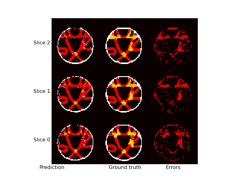
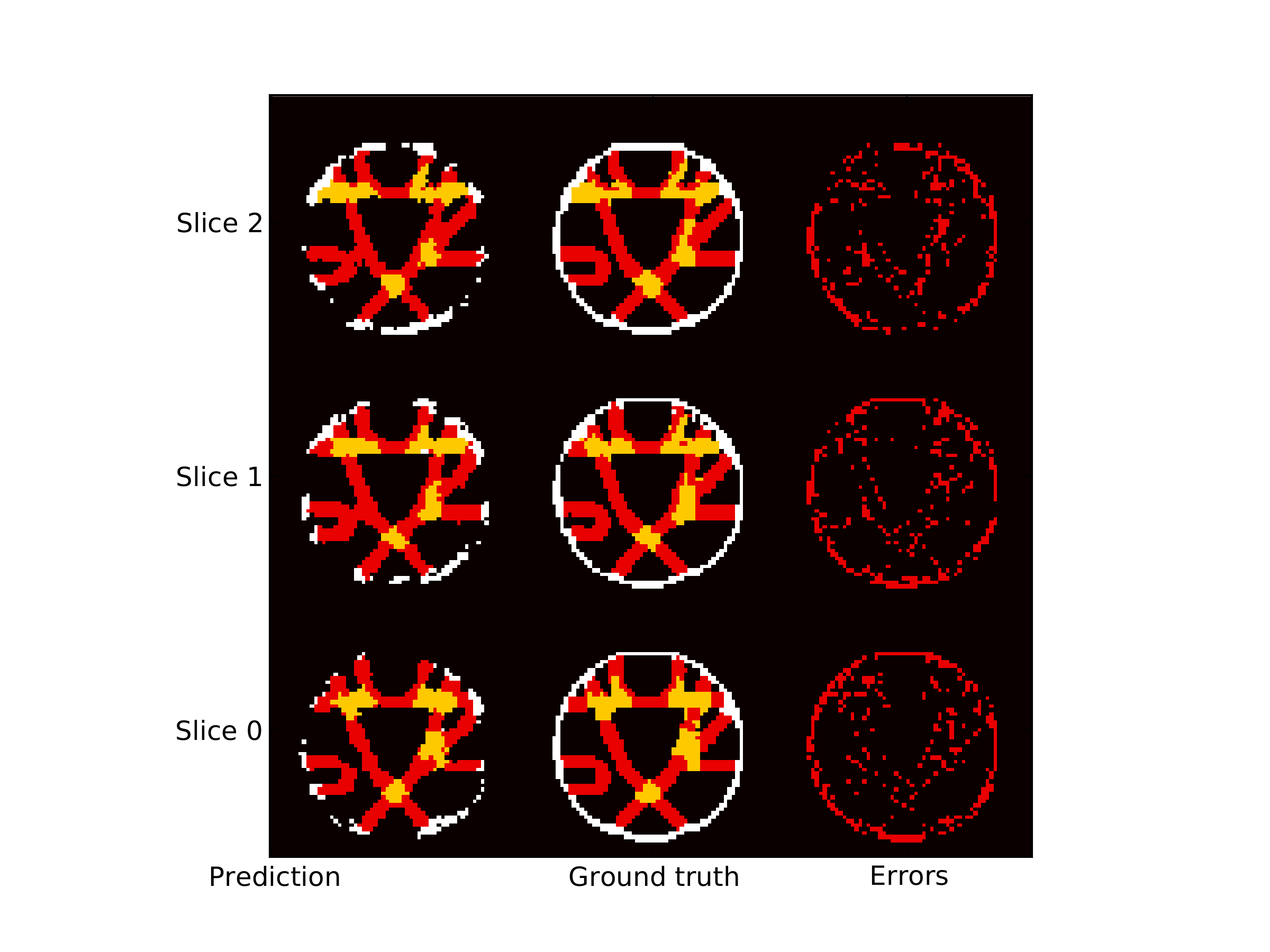
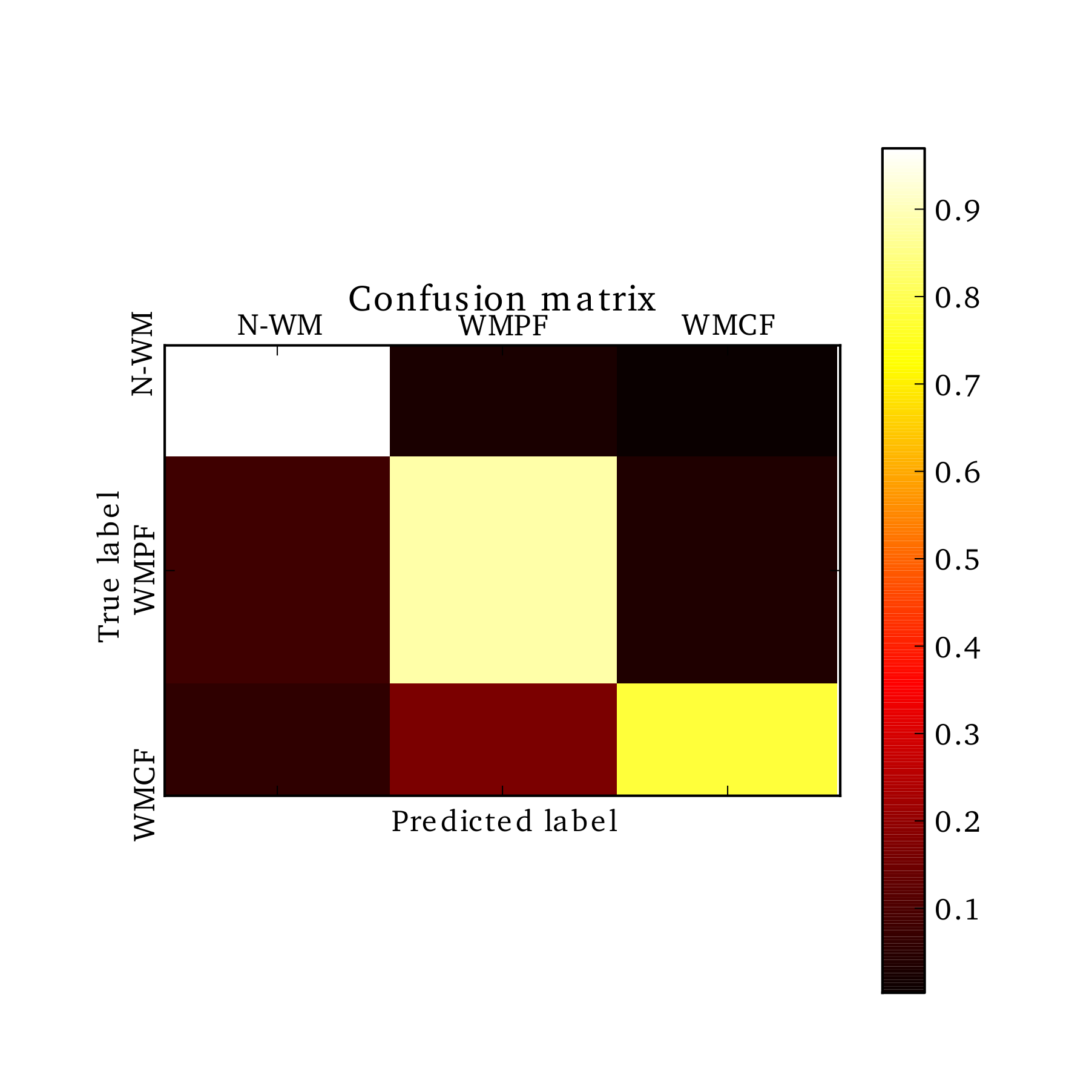
Tab. 1 presents the performances obtained using the best filter sets for each couple of features (SH4, SH8) and convolution kernel’s width (5, 7, 9) as well as the performances of the baseline classifiers. Fig. 3 visually presents the recognition performance using our method (SH8, kernel width of 5) against the best baseline classifier.
Baseline classifiers mainly do mistakes by detecting crossing fibers as single fibers. If we use the global classification error rates, they seem to perform well, however if we use the fitness value or look at Fig. 3a, we understand they perform badly. This may be explained because it is trained in order to reduce the global error rate whatever is the location of the errors. The proposed convolution based classifier performs better. Most error are miss recognition of the border of the phantom. This can be explained by the fact that the fitness function does not try to minimize this error. Most of the other errors are located at the frontier between two different classes. If we ignore the recognition error between CSF and GM (because there may not be important in our context), the error rate drops from 14.65% to 6.61% (SH8/window of size 5).
The huge amount of time involved in the experiment is not representative of a real use of the system as a lot of classifiers are learned and tried during the optimisation procedure. To give a more accurate representation of the duration of the computation, we have computed the mean time taken to learn the classifier and the mean time taken to classify the voxels by using the best kernels for each configuration of features and kernel width. It takes in average less than 11s to learn the classifier and a bit more than 1.50s to classify each voxel. In a real life application, only the classification process is used ; so we think it is fast enough to be used in a real world application even if processing time would be slightly larger with more voxels. We can approximate an overestimate of the classification duration of a whole brain by:
| (4) |
with V the number of voxels to classify. It is an overestimate as it does not take into account a potential reduction of the number of voxels to classify after having applyied a manual or automatic localisation of the brain. Thus with a matrix of , the classification duration would be approximatly . Ten minutes seems to be a correct amount of time.
4 Conclusion
We have proposed a new SVM classifier taking into account a local spatial neighbourhood to classify each voxel of HARDI data according to its water diffusion phenomenon. We can successfully classify voxels containing single fiber bundles, voxels with several directions of diffusion reflecting crossing fiber populations and random isotropic voxels without fiber bundles.
We believe that this opens many possible perspectives in quantitative white matter analysis in healthy and patients with neurodegenerative diseases. Future experiment could use large margin filtering [5] in order to optimize the SVM parameters while optimizing the convolution matrices. It is also important to apply the results on real brain datasets manually labelled by neurologists or neurosurgeons. Morphological operators could also decrease the recognition error rate.
References
- [1] T. E. J. Behrens, H. Johansen-Berg, S. Jbabdi, M. F. S. Rushworth, and M. W. Woolrich. Probabilistic diffusion tractography with multiple fibre orientations. what can we gain? NeuroImage, 34(1):144–155, 2007.
- [2] M. Descoteaux, E. Angelino, S. Fitzgibbons, and R. Deriche. Apparent Diffusion Coefficients from High Angular Resolution Diffusion Imaging: Estimation and Applications. Magnetic Resonance in Medicine, 56:395–410, 2006.
- [3] M. Descoteaux and C. Poupon. Diffusion-Weighted MRI. In Comprehensive Biomedical Physics, Elsevier, 2012.
- [4] P. Fillard, M. Descoteaux, A. Goh, S. Gouttard, B. Jeurissen, J. Malcolm, A. Ramirez-Manzanares, M. Reisert, K. Sakaie, F. Tensaouti, T. Yo, J.-F. cois Mangin, and C. Poupon. Quantitative evaluation of 10 tractography algorithms on a realistic diffusion mr phantom. NeuroImage, 56(1):220–234, 2011.
- [5] R. Flamary, D. Tuia, B. Labbé, G. Camps-Valls, and A. Rakotomamonjy. Large margin filtering. IEEE Transactions Signal Processing, 60(2):648–659, 2012.
- [6] B. Jeurissen, A. Leemans, J.-D. Tournier, D. K. Jones, and J. Sijbers. Investigating the prevalence of complex fiber configurations in white matter tissue with diffusion magnetic resonance imaging. Human Brain Mapping, in press(-):–, 2012.
- [7] V. Prčkovska, A. Vilanova, C. Poupon, B. M. Haar Romeny, and M. Descoteaux. Fast classification scheme for hardi data simplification. ICT Innovations 2009, pages 345–355, 2010.
- [8] S. Schnell, D. Saur, B. W. Kreher, J. Hennig, H. Burkhardt, and V. G. Kiselev. Fully automated classification of HARDI in vivo data using a support vector machine. NeuroImage, 46(3):642–651, 2009.
- [9] V. Vapnik et al. Theory of support vector machines. Department of Computer Science, Royal Holloway, University of London, pages 1677–1681, 1996.
- [10] S. B. Vos, D. K. Jones, B. Jeurissen, M. a. Viergever, and A. Leemans. The influence of complex white matter architecture on the mean diffusivity in diffusion tensor MRI of the human brain. NeuroImage, 59(3):2208–2216, Oct. 2012.
- [11] D. Wassermann, M. Descoteaux, and R. Deriche. Diffusion Maps Clustering for Magnetic Resonance Q-Ball Imaging Segmentation. International Journal on Biomedical Imaging, special issue on Recent Advances in Neuroimaging Methodology, 2008:–, 2008.
- [12] C.-F. Westin, S. E. Maier, H. Mamata, a. Nabavi, F. a. Jolesz, and R. Kikinis. Processing and visualization for diffusion tensor MRI. Medical image analysis, 6(2):93–108, June 2002.