Adaptive Equi-Energy Sampler: Convergence and Illustration

Abstract

Markov chain Monte Carlo (MCMC) methods allow to sample a distribution known up to a multiplicative constant. Classical MCMC samplers are known to have very poor mixing properties when sampling multimodal distributions. The Equi-Energy sampler is an interacting MCMC sampler proposed by Kou, Zhou and Wong in 2006 to sample difficult multimodal distributions. This algorithm runs several chains at different temperatures in parallel, and allow lower-tempered chains to jump to a state from a higher-tempered chain having an energy ‘close’ to that of the current state. A major drawback of this algorithm is that it depends on many design parameters and thus, requires a significant effort to tune these parameters.

In this paper, we introduce an Adaptive Equi-Energy (AEE) sampler which automates the choice of the selection mecanism when jumping onto a state of the higher-temperature chain. We prove the ergodicity and a strong law of large numbers for AEE, and for the original Equi-Energy sampler as well. Finally, we apply our algorithm to motif sampling in DNA sequences.

Keywords: interacting Markov chain Monte Carlo, adaptive sampler, equi-energy sampler, ergodicity, law of large numbers, motif sampling.

Author’s email addresses: first-name.last-name@telecom-paristech.fr

This work is partially supported by the French National Research Agency, under the program ANR-08-BLAN-0218 BigMC.

1 Introduction

Markov Chain Monte Carlo (MCMC) methods are well-known tools for sampling a target distribution $\pi$ known up to a multiplicative constant. MCMC algorithms sample $\pi$ by constructing a Markov chain admitting $\pi$ as unique invariant distribution. A canonical example is the the Metropolis-Hastings algorithm [27, 20]: given the current value $X_{n}$ of the chain $\{X_{j},\,j\geq 0\}$, it consists in proposing a move $Y_{n+1}$ under a proposal distribution $Q(X_{n},\cdot)$. This move is then accepted with probability

$$\alpha_{n}=1\wedge\pi(Y_{n+1})Q(Y_{n+1},X_{n})/[\pi(X_{n})Q(X_{n},Y_{n+1})]\;,$$

where $a\wedge b$ stands for $\min(a,b)$; otherwise, $X_{n+1}=X_{n}$.

It is known that the efficiency of MCMC methods depends upon the choice of the proposal distribution [31]. For example, when sampling multi-modal distributions, a Metropolis-Hastings algorithm with $Q(X_{n},\cdot)$ equal to a Gaussian distribution centered in $X_{n}$ tends to be stuck in one of the modes. So the convergence of such an algorithm will be slow, and the target distribution will not be correctly approximated unless a huge number of points is sampled.

Efficient implementations of MCMC rely on a strong expertise of the user in order to choose a proposal kernel and, more generally, design parameters adapted to the target $\pi$.

This is the reason why adaptive and interacting MCMC methods have been introduced. Adaptive MCMC methods consist in choosing, at each iteration, a transition kernel $P_{\theta}$ among a family $\{P_{\theta},\theta\in\Theta\}$ of kernels with invariant distribution $\pi$: the conditional distribution of $X_{n+1}$ given the past is $P_{\theta_{n}}(X_{n},\cdot)$ where the parameter $\theta_{n}$ is chosen according to the past values of the chain $\{X_{n},n\geq 0\}$. From the pioneering Adaptive Metropolis algorithm of [19], many adaptive MCMC have been proposed and successfully applied (see the survey papers by [5], [31], [6] for example).

Interacting MCMC methods rely on the (parallel) construction of a family of processes with distinct stationary distributions; the key behind these techniques is to allow interactions when sampling these different processes. At least one of these processes has $\pi$ as stationary distribution. The stationary distributions of the auxiliary processes are chosen in such a way that they have nice convergence properties, hoping that the process under study will inherit them. For example, in order to sample multi-modal distributions, a solution is to draw auxiliary processes with target distributions equal - up to the normalizing constant - to tempered versions $\pi^{1/T_{i}}$, $T_{i}>1$. This solution is the basis of the parallel tempering algorithm [18], where the states of two parallel chains are allowed to swap. Following this tempering idea, different interacting MCMC algorithms have been proposed and studied so far [1, 11, 14, 13].

The Equi-Energy sampler of Kou, Zhou and Wong [22] is an example of such interacting MCMC algorithms. $K$ processes are sampled in parallel, with target distributions (proportional to) $\pi^{\beta_{k}}$, $1=\beta_{K}>\beta_{K-1}>\cdots>\beta_{1}$. The first chain $Y^{(1)}=\{Y_{n}^{(1)},n\geq 0\}$ is usually a Markov chain; then $Y^{(k)}$ is built from $Y^{(k-1)}$ as follows: with a fixed probability $\varepsilon$, the current state $Y_{n}^{(k)}$ is allowed to jump onto a past state of the auxiliary chain $\{Y^{(k-1)}_{\ell},\ell\leq n\}$, and with probability $(1-\varepsilon)$, $Y_{n}^{(k)}$ is obtained using a “local" MCMC move (such as a random walk Metropolis step or a Metropolis-adjusted Langevin step). This mechanism includes the computation of an acceptance ratio so that the chain $Y^{(k)}$ will have $\pi^{\beta_{k}}$ as target density. As the acceptance probability of such a jump could be very low, only jumps toward selected past values of $Y^{(k-1)}$, namely those with an energy close to that of the current state $Y_{n}^{(k)}$, are allowed. This selection step allows higher acceptance rates of the jump, and a faster convergence of the algorithm is expected.

The Equi-Energy sampler has many design parameters: the interacting probability $\varepsilon$, the number $K$ of parallel chains, the temperatures $T_{k}=1/\beta_{k}$, $k\in\{1,\dots,K\}$ and the selection function. It is known that all of these design parameters play a role on the efficiency of the algorithm. [22] suggest some values for all these parameters, designed for practical implementation and based on empirical results on some simple models. [3] discuss the choice of the interacting probability $\varepsilon$ in similar contexts; [8] discuss the choice of the temperatures $T_{k}$ of the chains for the Parallel Tempering algorithm. Recently, an algorithm combining parallel tempering with equi-energy moves have been proposed by [10].

In this paper, we discuss the choice of the energy rings and the selection function, when the jump probability $\varepsilon$, the number $K$ of auxiliary processes and the temperatures are fixed. We introduce a new algorithm, called Adaptive Equi-Energy sampler in which the selection function is defined adaptively based on the past history of the sampler. We also address the convergence properties of this new sampler.

Different kinds of convergence of adaptive MCMC methods have been addressed in the literature: convergence of the marginals, the law of large numbers (LLN) and central limit theorems (CLT) for additive functionals (see e.g. [29] for convergence of the marginals and weak LLN of general adaptive MCMC, [4] or [34] for LLN and CLT for adaptive Metropolis algorithms, [16] and [17] for convergence of the marginals, LLN and CLT for general adaptive MCMC algorithms - see also the survey paper by [6]).

There are quite few analysis of the convergence of interacting MCMC samplers. The original proof of the convergence of the Equi-Energy sampler in [22] (resp. [7]) contains a serious gap, mentioned in [7] (resp. [2]). [3] established a strong LLN of a simplified version of the Equi-Energy sampler, in which the number of levels is set to $K=2$ and the proposal during the interaction step are drawn uniformly at random in the past of the auxiliary process. Finally, Fort, Moulines and Priouret [16] established the convergence of the marginals and a strong LLN for the same simplified version of the Equi-Energy sampler (with no selection) but have removed the limitations on the number of parallel chains.

The paper addresses the convergence of an interacting MCMC sampler in which the proposal are selected from energy rings which are constructed adaptively at each levels. In this paper, we obtain the convergence of the marginals and a strong LLN of a smooth version of the Equi-Energy sampler and its adaptive variant. We illustrate our results in several difficult scenarios such as sampling mixture models with “well-separated" modes and motif sampling in biological sequences. The paper is organized as follows: in Section 2, we derive our algorithm and set the notations that are used throughout the paper. The convergence results are presented in Section 3. Finally, Section 4 is devoted to the application to motif sampling in biological sequences. The proofs of the results are postponed to the Appendix.

2 Presentation of the algorithm

2.1 Notations

Let $(\mathbf{X},\mathcal{X})$ be a measurable Polish state space and $P$ be a Markov transition kernel on $(\mathbf{X},\mathcal{X})$. $P$ operates on bounded functions $f$ on $\mathbf{X}$ and on finite positive measures $\mu$ on $\mathcal{X}$:

$$Pf(x)=\int P(x,\mathrm{d}y)f(y),\qquad\mu P(A)=\int\mu(dx)P(x,A)\;.$$

The $n$-iterated transition kernel $P^{n}$, $n\geq 0$ is defined by:

$$P^{n}(x,A)=\int P^{n-1}(x,\mathrm{d}y)P(y,A)=\int P(x,\mathrm{d}y)P^{n-1}(y,A)\;;$$

by convention, $P^{0}(x,A)$ is the identity kernel. For a function $V:\mathbf{X}\rightarrow[1,+\infty[$, we denote by $|f|_{V}$ the V-norm of a function $f:\mathbf{X}\rightarrow\mathbb{R}$:

$$|f|_{V}=\sup_{x\in\mathbf{X}}\frac{|f(x)|}{V(x)}\;.$$

If $V=1$, this norm is the usual uniform norm. Let $\mathcal{L}_{V}=\{f:\mathbf{X}\rightarrow\mathbb{R},|f|_{V}<+\infty\}$. We also define the V-distance between two probability measures $\mu_{1}$ and $\mu_{2}$ by:

$$\|\mu_{1}-\mu_{2}\|_{V}=\sup_{f,|f|_{V}\leq 1}|\mu_{1}(f)-\mu_{2}(f)|\;.$$

When $V=1$, the V-distance is the total-variation distance and will be denoted by $\|\mu_{1}-\mu_{2}\|_{TV}$.

Let $(\Theta,\mathcal{T})$ be a measurable space, and $\{P_{\theta},\theta\in\Theta\}$ be a family of Markov transition kernels; $\Theta$ can be finite or infinite dimensional. It is assumed that for all $A\in\mathcal{X}$, $(x,\theta)\rightarrow P_{\theta}(x,A)$ is $(\mathcal{X}\otimes\mathcal{T}|\mathcal{B}([0,1]))$-measurable, where $\mathcal{B}([0,1])$ denotes the Borel $\sigma$-field on $[0,1]$.

2.2 The Equi-Energy sampler

Let $\pi$ be the probability density of the target distribution with respect to a dominating measure $\mu$ on $(\mathbf{X},\mathcal{X})$. In many applications, $\pi$ is known up to a multiplicative constant; therefore, we will denote by $\pi_{u}$ the (unnormalized) density.

We denote by $P$ the Metropolis-Hastings kernel with proposal density kernel $q$ and invariant distribution $\pi$ defined by:

$$P(x,A)=\int_{A}r(x,y)q(x,y)\mu(\mathrm{d}y)+\mathbf{1}_{A}(x)\int(1-r(x,y))q(x,y)\mu(\mathrm{d}y)\;,$$

where $(x,y)\mapsto r(x,y)$ is the acceptance ratio given by

$$r(x,y)=1\wedge\frac{\pi(y)q(y,x)}{\pi(x)q(x,y)}\;.$$

The Equi-Energy (EE) sampler proposed by [22] exploits the fact that it is often easier to sample a tempered version $\pi^{\beta}$, $0<\beta<1$, of the target distribution than $\pi$ itself. This is why the algorithm relies on an auxiliary process $\{Y_{n},n\geq 0\}$, run independently from $\{X_{n}\}$ and admitting $\pi^{\beta}$ as stationary distribution (up to a normalizing constant). This mechanism can be repeated yielding to a multi-stages Equi-Energy sampler.

We denote by $K$ the number of processes run in parallel. Let $\varepsilon\in(0,1)$. Choose $K$ temperatures $T_{1}>\dots>T_{K}=1$ and set $\beta_{k}=1/T_{k}$; and $K$ MCMC kernels $\{P^{(k)},1\leq k\leq K\}$ such that $\pi^{\beta_{k}}P^{(k)}=\pi^{\beta_{k}}$. $K$ processes $Y^{(k)}=\{Y_{n}^{(k)},n\geq 0\}$, $1\leq k\leq K$, are defined by induction on the probability space $(\Omega,\mathcal{F},\mathbb{P})$. The first auxiliary process $Y^{(1)}$ is a Markov chain, with $P^{(1)}$ as transition kernel. Given the auxiliary process $Y^{(k-1)}$ up to time $n$, $\{Y_{m}^{(k-1)},m\leq n\}$, and the current state $Y_{n}^{(k)}$ of the process of level $k$, the Equi-Energy sampler draws $Y_{n+1}^{(k)}$ as follows:

• (Metropolis-Hastings step) with probability $1-\varepsilon$, $Y_{n+1}^{(k)}\sim P^{(k)}(Y_{n}^{(k)},\cdot)$.

• (equi-energy step) with probability $\varepsilon$, the algorithm selects a state $Z_{n+1}$ from the auxiliary process having an energy close to that of the current state. An acceptance-rejection ratio is then computed and if accepted, $Y_{n+1}^{(k)}=Z_{n+1}$; otherwise, $Y_{n+1}^{(k)}=Y_{n}^{(k)}$.

In practice, [22] only apply the equi-energy step when there is at least one point in each ring. In [22], the distance between the energy of two states is defined as follows. Consider an increasing sequence of positive real numbers

$$\xi_{0}=0<\xi_{1}<\dots<\xi_{S}=+\infty\;.$$ (1)

If the energies of two states $x$ and $y$ belong to the same energy ring, i.e. if there exists $1\leq\ell\leq S$ such that $\xi_{\ell-1}\leq\pi_{u}(x),\pi_{u}(y)<\xi_{\ell}$, then the two states are said to have “close energy”. The choice of the energy rings is most often a difficult task. As shown in Figure 3[right], the Equi-Energy sampler is inefficient when the energy rings are not appropriately defined. The efficiency of the sampler is increased when the variation of $\pi_{u}$ in each ring is small enough so that the equi-energy move is accepted with high probability.

2.3 The Adaptive Equi-Energy sampler

We propose to modify the Equi-Energy sampler by adapting the energy rings “on the fly", based on the history of the algorithm. Our new algorithm, so called Adaptive Equi-Energy sampler (AEE) is similar to the Equi-Energy sampler of [22] except for the equi-energy step, which relies on adaptive boundaries of the rings. For the definition of the process $Y^{(k)}$, $k\geq 2$, adaptive boundaries computed from the process $Y^{(k-1)}$ are used.

For a distribution $\theta$ in $\Theta$, denote by $\xi_{\theta,\ell}$, $\ell\in\{1,\cdots,S-1\}$ the bounds of the rings, computed from r.v. with distribution $\theta$; by convention, $\xi_{\theta,0}=0\leq\xi_{\theta,1}\leq\cdots\leq\xi_{\theta,S-1}\leq\xi_{\theta,S}=+\infty$. Define the associated energy rings $H_{\theta,\ell}=[\xi_{\theta,\ell-1},\xi_{\theta,\ell})$ for $\ell\in\{1,\cdots,S\}$. We consider selection functions $g_{\theta}(x,y)$ of the form

$$g_{\theta}(x,y)=\sum_{\ell=1}^{S}h_{\theta,\ell}(x)h_{\theta,\ell}(y)\;,\quad h_{\theta,\ell}(x)=\left(1-d(\pi_{u}(x),H_{\theta,\ell})\right)_{+}\;,$$ (2)

where $d(\pi_{u}(x),H_{\theta,\ell})$ measures the distance between $\pi_{u}(x)$ and the ring $H_{\theta,\ell}$. By convention $h_{\theta,\ell}=0$ if $H_{\theta,\ell}=\emptyset$. We finally introduce a set of selection kernels $\{K_{\theta}^{(k)},\theta\in\Theta\}$ for all $k\in\{2,\cdots,K\}$ defined by

$$K_{\theta}^{(k)}(x,A) =\int_{A}\alpha_{\theta}^{(k)}(x,y)\frac{g_{\theta}(x,y)\theta(\mathrm{d}y)}{\int g_{\theta}(x,z)\theta(\mathrm{d}z)}+\mathbf{1}_{A}(x)\int\{1-\alpha_{\theta}^{(k)}(x,y)\}\frac{g_{\theta}(x,y)\theta(\mathrm{d}y)}{\int g_{\theta}(x,z)\theta(\mathrm{d}z)}\;,$$ (3)

where

$$\alpha_{\theta}^{(k)}(x,y)=1\wedge\left(\frac{\pi^{\beta_{k}-\beta_{k-1}}(y)\int g_{\theta}(x,z)\theta(\mathrm{d}z)}{\pi^{\beta_{k}-\beta_{k-1}}(x)\int g_{\theta}(y,z)\theta(\mathrm{d}z)}\right)\;.$$ (4)

$K_{\theta}^{(k)}$ is associated to the equi-energy step when defining $Y^{(k)}$: a draw under the selection kernel proportional to $g_{\theta}(x,y)\theta(\mathrm{d}y)$ is combined with an acceptance-rejection step. The acceptance-rejection step is defined so that when $\theta\propto\pi^{\beta_{k-1}}$, $\pi^{\beta_{k}}$ is invariant for $K_{\theta}^{(k)}$ [22].

This equi-energy step is only allowed when each ring contains at least one point (of the auxiliary process $Y^{(k-1)}$ up to time $n$). We therefore introduce, for all positive integer $m$, the set ${\Theta}_{m}$:

$${\Theta}_{m}\stackrel{{\scriptstyle\mathrm{def}}}{{=}}\left\{\theta\in\Theta:\frac{1}{m}\leq\inf_{x}\int g_{\theta}(x,y)\theta(\mathrm{d}y)\right\}\;.$$ (5)

With these notations, AEE satisfies for any $n\geq 0$ and $k\in\{1,\cdots,K\}$,

$$\mathbb{E}[f(Y_{n+1}^{(k)})|\mathcal{F}_{n}^{(k)}]=\mathbb{E}[f(Y_{n+1}^{(k)})|Y_{n}^{(k)},Y_{m}^{(k-1)},1\leq m\leq n]=P_{\theta_{n}^{(k-1)}}^{(k)}f(Y_{n}^{(k)})\;,$$ (6)

where $\{\mathcal{F}_{n}^{(k)},n\geq 0\}$ is the filtration defined by $\mathcal{F}_{n}^{(k)}=\sigma\left(\left\{Y_{m}^{(l)},1\leq m\leq n,1\leq l\leq k\right\}\right)$; the transition kernel is given by $P_{\theta}^{(1)}=P^{(1)}$ and for $k\geq 2$,

$$P_{\theta}^{(k)}=(1-\varepsilon\mathbf{1}_{\theta\in\bigcup_{m\geq 1}\Theta_{m}})P^{(k)}+\varepsilon\mathbf{1}_{\theta\in\bigcup_{m\geq 1}\Theta_{m}}\ K_{\theta}^{(k)}\;;$$

and $\theta_{n}^{(k)}$ is the empirical distribution

$$\theta_{n}^{(k)}=\frac{1}{n}\sum_{m=1}^{n}\delta_{Y_{m}^{(k)}}\;,\qquad k\in\{1,\cdots,K\},n\geq 1\;.$$ (7)

Different functions $d$ can be chosen. For example, the function given by

$$d(\pi_{u}(x),H_{\theta,\ell})=\mathbf{1}_{\mathbb{R}\setminus H_{\theta,\ell}}(\pi_{u}(x))=\left\{\begin{array}[]{ll}0&\text{if}\ \pi_{u}(x)\in H_{\theta,\ell},\\ 1&\text{otherwise}\end{array}\right.$$ (8)

yields to a selection function $g_{\theta}$ such that $g_{\theta}(x,y)=1$ iff $x,y$ are in the same energy ring and $g_{\theta}(x,y)=0$ otherwise. In this case, the acceptance-rejection ratio $\alpha_{\theta}^{(k)}(x,y)$ is equal to $1\wedge(\pi^{\beta_{k}-\beta_{k-1}}(y)/\pi^{\beta_{k}-\beta_{k-1}}(x))$ upon noting that by definition of the proposal kernel, the points $x$ and $y$ are in the same energy ring. By using this “hard" distance during the equi-energy jump, all the states of the auxiliary process having their energy in the same ring as the energy of the current state are chosen with the same probability, while the other auxiliary states have no chance to be selected.

Other functions $d$ could be chosen, such as “soft" selections of the form

$$d(\pi_{u}(x),H_{\theta,l})=\frac{1}{r}\min_{y\in H_{\theta,\ell}}|\pi_{u}(x)-y|\;,$$ (9)

where $r>0$ is fixed. With this “soft” distance, given a current state $Y_{n}^{(k)}$, the probability for each auxiliary state $Y_{i}^{(k-1)}$, $i\leq n$, to be chosen is proportional to $g_{\theta_{n}^{(k-1)}}(Y_{n}^{(k)},Y_{i}^{(k-1)})$. Then, the “soft" selection function allows auxiliary states having an energy in a $r$-neighborhood of the energy ring of $\pi_{u}(Y_{n}^{(k)})$ to be chosen, as well as states having their energy in this ring. Nevertheless, this selection function yields an acceptance-rejection ratio $\alpha_{\theta}^{(k)}$ which may reveal to be quite costly to evaluate.

The asymptotic behavior of AEE will be addressed in Section 3. The intuition is that when the empirical distribution $\theta_{n}^{(k-1)}$ of the auxiliary process of order $k-1$ converges (in some sense) to $\theta_{\star}^{(k-1)}$, the process $\{Y_{n}^{(k)},n\geq 0\}$ will behave (in some sense) as a Markov chain with transition kernel $P_{\theta_{\star}^{(k-1)}}^{(k)}$.

2.4 A toy example (I)

To highlight the interest of our algorithm, we consider toy examples: the target density $\pi$ is a mixture of $\mathbb{R}^{d}$-valued Gaussian . This model is known to be difficult, as illustrated (for example) in [6] for a random walk Metropolis-Hastings sampler (SRWM), an EE-sampler and a parallel tempering algorithm. Indeed, if the modes are well separated, a Metropolis-Hastings algorithm using only “local moves" is likely to remain trapped in one of the modes for a long-period of time. In the following, AEE is implemented with ring boundaries computed as described in Section 3.3.

Figure 1.(a) displays the target density $\pi$ and the simulated one for three different algorithms (SRWM, EE and AEE) in one dimension. The histograms are obtained with $10^{5}$ samples; for EE and AEE, the probability of interaction is $\varepsilon=0.1$, the number of parallel chains is equal to $K=5$ and the number of rings is $S=5$. For the adaptive definition of the rings in AEE, we choose the “hard" selection (8) and the construction of the rings defined in Section 3.3. In the same vein, Figure 2 displays the points obtained by the three algorithms when sampling a mixture of two Gaussian distributions in two dimensions. As expected, in both figures, SRWM never explores one of the modes, while EE and AEE are far more efficient.

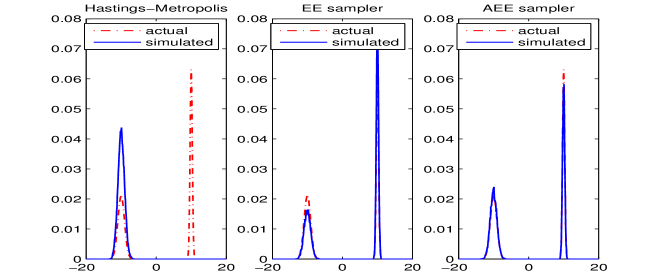
Figure 1: Comparison of SRWM (left), EE (center) and AEE (right) for a Gaussian mixture in one dimension

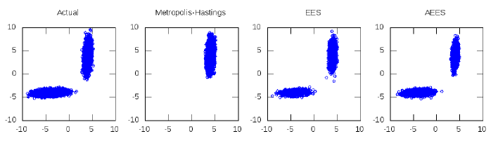
Figure 2: Comparison of the algorithms for a Gaussian mixture in two dimensions: (from left to right) the true density, SRWM, EE and AEE.

To compare EE and AEE in a more challenging situation, we consider the case of a mixture with two components in ten dimensions. We run EE and AEE with $K=3$ parallel chains with respective temperatures $T_{1}=1,T_{2}=9,T_{3}=60$, the probability of jump $\varepsilon$ is equal to $0.1$, and the number of rings is $S=50$. Both algorithms are initialized in one of the two modes of the distribution. For the Metropolis-Hastings step, we use a Symmetric Random Walk with Gaussian proposal; the covariance matrix of the proposal is of the form $c\ I$ where $c$ is calibrated so that the mean acceptance rate is approximatively $0.25$. Figure 3 displays, for each algorithm, the $L^{1}$-norm of the empirical mean, averaged over $10$ independent trajectories, as a function of the length of the chains.

In order to show that the efficiency of EE depends crucially upon the choice of the rings, we choose a set of boundaries so that in practice, along one run of the algorithm, some of the rings are never reached. Figure 3(a) compares EE and AEE in this extreme case: even after $2\times 10^{5}$ iterations, all of the equi-energy jumps are rejected for the (non-adaptive) EE, and the algorithm is trapped in one of the modes. This does not occur for AEE, and the $L^{1}$-error tends to zero as the number of iterations increases. This illustrates that our adaptive algorithm avoids the poor behaviors that EE can have when the choice of its design parameters is inappropriate.

We now run EE in a less extreme situation: we choose (fixed) energy rings so that the sampler can jump more easily than in the previous experiment between the modes. Figure 3(b) illustrates that the adaptive choice of the energy rings speeds up the convergence, as it makes the equi-energy jumps be more often accepted. To have a numerical comparison, the equi-energy jumps were accepted about ten times more often for AEE than for EE.

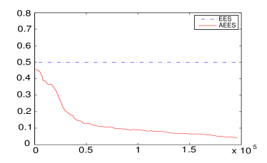
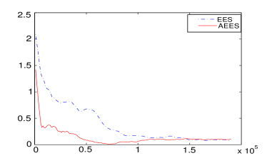
(a)	(b)

Figure 3: Error of EE (dashed line) and AEE for two different target densities in ten dimensions.

2.5 Toy example (II)

For a better understanding on how our algorithm behaves, Figure 4.(a) displays the evolution of the ring bounds used in the definition of $Y^{(K)}$. In this numerical application, the target density is a mixture of two Gaussian distributions in one dimension; EE and AEE are run with $K=5$ chains, $S=5$ rings and $\varepsilon=0.1$, for a number of iterations varying from $0$ to $10^{5}$. As expected, the ring bounds become stable after a reasonable number of iterations. Moreover, we observed that the (non-adaptive) EE run with the rings fixed to the limiting values obtained with AEE behaves remarkably well.

Finally, to have an idea on the role played by $\varepsilon$, Figure 4.(b) displays the average $L^{1}$ error of AEE for a mixture of two Gaussian distributions in one dimension, after $2\times 10^{5}$ iterations and for 100 independent trajectories when $\varepsilon$ is varying from 0 to 1. If $\varepsilon$ is too small, AEE is not mixing well enough, and if $\varepsilon$ is too large, the algorithm jumps easily from one mode to another but does not explore well enough each mode, which explains the ‘u’ shape of the curve. This experiment suggests that there exists an optimal value for $\varepsilon$, but to our best knowledge, the optimal choice of this design parameter is an open problem.

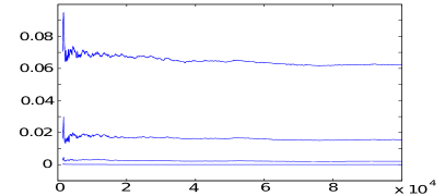
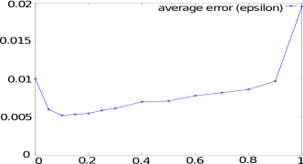
(a)	(b)

Figure 4: (a): Evolution of the ring bounds; (b): Averaged error of AEE as a function of $\varepsilon$.

3 Convergence of the Adaptive Equi-Energy sampler

In this section, the convergence of the $K$-stages Adaptive Equi-Energy sampler is established. In order to make the proof easier, we consider the case when the distance function $d$ in the definition of the selection function (2) is given by (9).

[16] provide sufficient conditions for the convergence of the marginals and the strong LLN (s-LLN) of interacting MCMC samplers. We use their results and show the convergence of the marginals i.e.

$$\lim_{n\rightarrow\infty}\mathbb{E}\left[f(Y_{n}^{(K)})\right]=\pi(f)\;,$$

for any continuous bounded functions $f$. Note that this implies that this limit holds for any indicator function $f=\mathbf{1}_{A}$ such that $\mathbb{P}(\partial A)=0$ where $\partial A$ denotes the boundary of $A$ [12, Theorem 2.1]. We then establish the s-LLN: for a wide class of continuous (un)bounded functions $f$,

$$\lim_{n\rightarrow\infty}\frac{1}{n}\sum_{m=0}^{n-1}f(Y_{m}^{(K)})=\pi(f)\;,\mathbb{P}-\mathrm{a.s.}$$

3.1 Assumptions

Our results are established for target distributions $\pi$ satisfying

• 1. $\pi$ is the density of a probability distribution on the measurable Polish space $(\mathbf{X},\mathcal{X})$ and $\sup_{\mathbf{X}}\pi<\infty$ and for any $s\in(0,1]$, $\int\pi^{s}(x)\ \mathrm{d}x<\infty$.

  2. $\pi$ is continuous and positive on $\mathbf{X}$.

Usually, the user knows $\pi$ up to a normalizing constant: hereafter, $\pi_{u}$ will denote this available (unnormalized) density.

As in [16], we first introduce a set of conditions that will imply the geometric ergodicity of the kernels $P_{\theta}^{(k)}$, and the existence of an invariant probability measure for $P_{\theta}^{(k)}$ (see conditions EE2). We finally introduce conditions on the boundaries of the adaptive energy rings (see conditions EE3). Examples of boundaries satisfying EE3 and computed from quantile estimators are given in Section 3.3 (see also [35] for stochastic approximation-based adapted boundaries).

Convergence of adaptive and interacting MCMC samplers is addressed in the literature by assuming containment conditions and diminishing adaptations (so called after [29]). Assumptions EE2 is the main tool to establish a (generalized) containment condition. In our algorithm, the adaptation mechanism is due to (a) the interaction with an auxiliary process and (b) the adaption of the rings. Therefore, assumptions EE2 and EE3 are related to the diminishing adaptation condition (see e.g. Lemma B.6 in Section B.3).

• For each $k\in\{1,\dots,K\}$:

  1. $P^{(k)}$ is a $\phi$-irreducible transition kernel which is Feller on $(\mathbf{X},\mathcal{X})$ and such that $\pi^{\beta_{k}}P^{(k)}=\pi^{\beta_{k}}$.

  2. There exist $\lambda_{k}\in(0,1)$, $b_{k}<+\infty$ and $\tau_{k}\in\left(0,\tau_{k-1}\beta_{k-1}/\beta_{k}\right)$ such that $P^{(k)}W_{k}\leq\lambda_{k}W_{k}+b_{k}$ with

     $$W_{k}(x)=\left(\frac{\pi^{\beta_{k}}(x)}{\sup_{\mathbf{X}}\pi^{\beta_{k}}}\right)^{-\tau_{k}}\;;$$ (10)

     by convention, $\tau_{0}\beta_{0}=\beta_{1}$.

  3. For all $p\in(0,\sup_{\mathbf{X}}\pi)$, the sets $\{\pi\geq p\}$ are 1-small for $P^{(k)}$.

Note that by definition of $\tau_{k}$ and EE1a, $W_{k+1}\in\mathcal{L}_{W_{k}}$ and $\int W_{k}(x)\pi^{\beta_{k}}(x)\mathrm{d}x<\infty$.

EE2 is satisfied for example if for each $k$, $P^{(k)}$ is a symmetric random walk Metropolis Hastings kernel; and $\pi$ is a sub-exponential target density [30, 21].

In our algorithm, $Y^{(1)}$ is a Markov chain with transition kernel $P^{(1)}$. As discussed in [28][chapters 13 and 17], EE2 is sufficient to prove ergodicity and a s-LLN for $Y^{(1)}$. EE2 also implies uniform $W_{1}$-moments for $Y^{(1)}$. These results, which initializes our proof by recurrence of the convergence for the process number $K$, is given in Proposition 3.1. Define the probability distributions

$$\theta_{\star}^{(k)}(\mathrm{d}x)=\frac{\pi^{\beta_{k}}(x)}{\int\pi^{\beta_{k}}(z)\mu(\mathrm{d}z)}\mu(\mathrm{d}x)\;,\qquad k\in\{1,\cdots,K\}\;.$$ (11)

Proposition 3.1.

Assume EE1a, EE2 and $\mathbb{E}\left[W_{1}(Y_{0}^{(1)})\right]<\infty$. Then,

1. For all bounded measurable functions $f$, $\lim_{n\to\infty}\mathbb{E}\left[f(Y_{n}^{(1)})\right]=\theta_{\star}^{(1)}(f)$.

2. $\theta_{\star}^{(1)}(W_{2})<+\infty$, and for any measurable function $f$ in $\mathcal{L}_{W_{1}}$, $\lim_{n\to\infty}\theta_{n}^{(1)}(f)=\theta_{\star}^{(1)}(f)$ a.s.

3. $\sup_{n}\mathbb{E}\left[W_{1}\left(Y_{n}^{(1)}\right)\right]<\infty$.

• 1. For any $k\in\{1,\dots,K-1\}$, $\inf_{\ell\in\{1,\cdots,S-1\}}\int h_{\theta_{\star}^{(k)},\ell}(y)\ \theta_{\star}^{(k)}(\mathrm{d}y)>0$.

  2. For any $k\in\{1,\dots,K-1\}$ and $\ell\in\{1,\cdots,S-1\}$, $\lim_{n\to\infty}\left|\xi_{\theta_{n}^{(k)},\ell}-\xi_{\theta_{\star}^{(k)},\ell}\right|=0$ w.p.1

  3. There exists $\Gamma>0$ such that for any $k\in\{1,\dots,K-1\}$, any $\ell\in\{1,\cdots,S-1\}$, and any $\gamma\in(0,\Gamma)$, $\limsup_{n}\ n^{\gamma}\ \left|\xi_{\theta_{n+1}^{(k)},\ell}-\xi_{\theta_{n}^{(k)},\ell}\right|<\infty$ w.p.1.

Note that by definition of $h_{\theta,\ell}$ (see (2))

$$\int h_{\theta,\ell}(y)\ \theta(\mathrm{d}y)\geq\theta(\{y:\pi_{u}(y)\in H_{\theta,\ell}\})\;.$$ (12)

Condition EE3b states that the rings $\{H_{\theta_{n}^{(k)},\ell)},n\geq 0\}$ converge to $H_{\theta_{\star}^{(k)},\ell}$ w.p.1; therefore, EE3a is satisfied as soon as the limiting rings are of positive probability under the distribution of $\pi_{u}(Z)$ when $Z\sim\theta_{\star}^{(k)}$.

When the energy bounds are fixed, the conditions EE3b-c are clearly satisfied and EE3a holds under convenient choice of the rings. We will discuss in Section 3.3 how to check the condition EE3 with adaptive energy bounds.

3.2 Convergence results

Proposition 3.2 shows that the kernels $P_{\theta}^{(k)}$ satisfy a geometric drift inequality and a minorization condition, with constants in the drift independent of $\theta$ for $\theta\in\Theta_{m}$ ($\Theta_{m}$ being defined in (5)). The proof is in Appendix A.1.

Proposition 3.2.

Assume EE1a and EE2. For all $k\in\{1,\dots,K\}$:

1. There exist $\tilde{\lambda}_{k}\in(0,1)$ and $\tilde{b}_{k}<+\infty$ such that for all $m\geq 1$ and any $\theta\in\Theta_{m}$,

   $$P_{\theta}^{(k)}W_{k}\leq\tilde{\lambda}_{k}W_{k}+\tilde{b}_{k}\ m\,\theta(W_{k})\ \;.$$ (13)

   For all $p\in(0,\sup_{\mathbf{X}}\pi)$ and all $\theta\in\bigcup_{m}\Theta_{m}$, the sets $\{\pi\geq p\}$ are $1$-small for $P_{\theta}^{(k)}$ and the minorization constants depend neither upon $\theta$ nor on $m$.

2. For all $\theta\in\bigcup_{m}\Theta_{m}$, there exists a probability measure $\pi_{\theta}^{(k)}$ invariant for $P_{\theta}^{(k)}$. In addition, $\pi_{\theta}^{(k)}(W_{k})\leq\tilde{b}_{k}(1-\tilde{\lambda}_{k})^{-1}\ m\theta(W_{k})$ for $\theta\in\Theta_{m}$.

Theorem 3.3 is proved in Section B. Theorem 3.3(a) shows that there exists $m_{\star}\geq 1$ such that w.p.1, for all $n$ large enough $\theta_{n}^{(k)}$ belongs to some $\Theta_{m_{\star}}$. Note that in [2], a s-LLN for the Equi-Energy sampler is established by assuming that there exists a deterministic positive integer $m$ such that w.p.1, $\theta_{n}^{(k)}\in\Theta_{m}$ for any $n$. Such a condition is quite strong since roughly speaking, it means that after $n$ steps (even for small $n$), all the rings contain a number of point which is proportional to $n$, w.p.1. This is all the more difficult to guarantee in practice, that the rings have to be chosen prior to any exploration of $\pi$. Our approach allows to relax this strong condition.

The convergence of the marginals and the law of large numbers both require the convergence in $n$ ($k$ fixed) of $\{\pi_{\theta_{n}^{(k)}}^{(k+1)}(f),n\geq 0\}$ for some functions $f$. Such a convergence is addressed in Theorem 3.3(b). We will then have the main ingredients to establish the convergence results for the processes $Y^{(k)}$, $k\geq 1$.

Theorem 3.3.

Assume EE1, EE2, EE3 and $\mathbb{E}[W_{k}(Y_{0}^{(k)})]<\infty$ for all $k\in\{1,\cdots,K\}$.

1. There exists $m_{\star}\geq 1$ such that for all $k\in\{1,\dots,K-1\}$

   $$\mathbb{P}\left(\bigcup_{q\geq 1}\bigcap_{n\geq q}\{\theta_{n}^{(k)}\in\Theta_{m_{\star}}\}\right)=1\;.$$ (14)

2. For any $k\in\{1,\cdots,K\}$, any $a\in(0,1)$ and any continuous function $f\in\mathcal{L}_{W_{k}^{a}}$,

   $$\lim_{n\to\infty}\pi_{\theta_{n}^{(k-1)}}^{(k)}(f)=\theta_{\star}^{(k)}(f)\;,\ \text{w.p.1}\;.$$

3. For any $k\in\{1,\cdots,K\}$ and for all bounded continuous function $f:\mathbf{X}\to\mathbb{R}$, $\lim_{n\to\infty}\mathbb{E}[f(Y_{n}^{(k)})]=\theta_{\star}^{(k)}(f)$.

4. Let $a\in(0,\frac{1+\Gamma}{2}\wedge 1)$. For any $k\in\{1,\cdots,K\}$ and for all continuous function $f$ in $\mathcal{L}_{W_{k}^{a}}$

   $$\lim_{n\to\infty}\frac{1}{n}\sum_{m=1}^{n}f(Y_{m}^{(k)})=\theta_{\star}^{(k)}(f)\qquad\mathbb{P}-\text{a.s.}\;.$$

Observe that, for the process $\{Y^{(k)},k\in\mathbb{N}\}$, the family of functions for which the law of large numbers holds depends (i) upon $\Gamma$ given by EEE3(c) i.e. in some sense, depends upon the adaptation rate; and (ii) the temperature ladder. In the case $\tau_{k}$ can be chosen arbitrarily close to $\beta_{1}/\beta_{k}$ for any $k$ (see comments after [21, Theorem 4.1 and 4.3]), this family of functions only depends upon $\Gamma$ and the lowest inverse temperature : it is all the more restrictive than $\beta_{1}$ is small.

To our best knowledge, we are the first to prove such convergence results for AEE (and EE): previous works [16, 3] consider the simpler case when there is no selection i.e. $g_{\theta}(x,y)=1$.

3.3 Comments on Assumption EE3

We propose to choose the adaptive boundaries $\xi_{\theta,\ell}$ as the $p_{\ell}$-quantile of the distribution of $\pi_{u}(Z)$ when $Z$ is sampled under the distribution $\theta$. This section proves that empirical quantiles of regularly spaced orders are examples of adaptive boundaries $\xi_{\theta_{n}^{(k)},\ell}$ satisfying EE3. Let $F_{\theta}$ be the cumulative distribution function (cdf) of the r.v. $\pi_{u}(Z)$ when $Z\sim\theta$:

$$F_{\theta}(x)=\int\mathbf{1}_{\{\pi_{u}(z)\leq x\}}\theta(\mathrm{d}z)\;,\qquad x\in[0,\infty)\;.$$

We denote the quantile function associated to $\pi_{u}(Z)$ by:

$$F_{\theta}^{-1}(p)=\inf\{x\geq 0,F_{\theta}(x)\geq p\}\quad\forall p>0\;;\qquad\qquad F_{\theta}^{-1}(0)=0\;.$$

With this definition, for $0<p_{1}<\cdots<p_{S-1}<1$, we set $\xi_{\theta,\ell}\stackrel{{\scriptstyle\mathrm{def}}}{{=}}F_{\theta}^{-1}\left(p_{\ell}\right)$.

With this choice of the boundaries, the condition EE3a holds: by (12), EE3a is satisfied because $\pi$ is continuous. The conditions EE3b-c require the convergence of the quantile estimators and a rate of convergence of the variation of two successive boundaries. To prove such conditions, we use an Hoeffding-type inequality.

Proposition 3.4.

Assume

1. The cumulative distribution function $F_{\theta_{\star}^{(1)}}$ where $\theta_{\star}^{(1)}$ is given by (11), is differentiable with positive derivative on $F_{\theta_{\star}^{(1)}}^{-1}((0,1))$.

2. there exists $\overline{W}$ such that $Y^{(1)}$ is a $\overline{W}$-uniformly ergodic Markov chain with initial distribution satisfying $\mathbb{E}\left[Y^{(1)}_{0}\right]<\infty$.

Then EE3b-c hold with $\Gamma=1/2$ and $K=2$.

The proof is in Section B.5. Extensions of Proposition 3.4 to the case when $Y^{(1)}$ is not a uniformly ergodic Markov chain is, to our best knowledge, an open question. Therefore, our convergence result of AEE when the boundaries are the quantiles defined by inversion of the cdf of the auxiliary process applies to the $2$-stage level and seems difficult to extend to the $K$-stage, $K>2$.

We proved recently in [35] that when the quantiles are defined by a stochastic approximation procedure, the conditions EE3b-c hold even under very weak conditions on the auxiliary $Y^{(k)}$, $k\geq 2$. In this case, the convergence of the $K$-level AEE with $K>2$ is established.

4 Application to motif sampling in biological sequences

One of the challenges in biology is to understand how gene expression is regulated. Biologists have found that proteins called transcription factors play a role in this regulation. Indeed, transcription factors bind on special motifs of DNA and then attract or repulse the enzymes that are responsible of transcription of DNA sequences into proteins. This is the reason why finding these binding motifs is crucial. But binding motifs do not contain deterministic start and stop codons: they are only random sequences that occurs more frequently than expected under the background model.

Several methods have been proposed so far to retrieve binding motifs [36, 24, 9], which yields to a complete Bayesian model [25]. Among the Bayesian approach, one effective method is based on the Gibbs sampler [23] - it has been popularized by software programs [26, 33]. Nevertheless, as discussed in [22], it may happen that classical MCMC algorithms are inefficient for this Bayesian approach. Therefore, [22] show the interest of the Equi-Energy sampler when applied to this Bayesian inverse problem; more recently, [32] proposed a Gibbs-based algorithm for a similar model (their model differs from the following one through the assumptions on the background sequence).

We start with a description of our model for motif sampling in biological sequences - this section is close to the description in  [22] but is provided to make this paper self-contained. We then apply AEE and compare it to the Interacting MCMC of [16, Section 3] (hereafter called I-MCMC), and to a Metropolis-Hastings algorithm (MH). Comparison with Gibbs-based algorithms (namely BioProspector and AlignACE) can be found in the paper of [22].

The available data is a DNA sequence, which is modeled by a background sequence in which some motifs are inserted. The background sequence is represented by a vector $\mathsf{S}=(s_{1},s_{2},\dots,s_{L})$ of length $L$. Each element $s_{i}$ is a nucleotide in $\{A,C,G,T\}$; in this paper, we will choose the convention $s_{i}\in\{1,2,3,4\}$. The length $w$ of a motif is assumed to be known. The motif positions are collected in a vector $A=(a_{1},\dots,a_{L})$, with the convention that $a_{i}=j$ iff the nucleotide $s_{i}$ is located at position number $j$ of a motif; and $a_{i}=0$ iff $s_{i}$ is not in the motif. The goal of the statistical analysis of the data $\mathsf{S}$ is to explore the distribution of $A$ given the sequence $\mathsf{S}$. We now introduce notations and assumptions on the model in order to define this conditional distribution.

We denote by $p_{0}$ the probability that a sub-sequence of length $w$ of $\mathsf{S}$ is a motif. It is assumed that the background sequence is a Markov chain with (deterministic) transition matrix $v_{0}=\{v_{0}(i,j)\}_{1\leq i,j\leq 4}$ on $\{1,\cdots,4\}$; and the nucleotide in a sequence are sampled from a multinomial distribution of parameter $v=\{v(i,j)\}_{1\leq i\leq 4,1\leq j\leq w}$ , $v(i,j)$ being the probability for the $j$-th element of a motif to be equal to $i$.

In practice, it has been observed that approximating $v_{0}(i,j)$ by the frequency of jumps from $i$ to $j$ in the (whole) sequence $\mathsf{S}$ is satisfying. It is assumed that the r.v. $(v,p_{0})$ are independent with prior distribution $\prod_{j=1}^{w}\chi(v(\cdot,j))$ and $\chi^{\prime}(p_{0})$; $\chi(v(\cdot,j))$ is a Dirichlet distribution with parameters $\iota_{j}=(\iota_{j,1},\cdots,\iota_{j,4})$ and $\chi^{\prime}(p_{0})$ is a Beta distribution with parameters $(b_{1},b_{2})$. $\iota_{j}$, $b_{1}$ and $b_{2}$ are assumed to be known.

Therefore, given $(v,p_{0})$, $(A,\mathsf{S})$ is a Markov chain described as follows:

• If $a_{k-1}\in\{1,\dots,w-1\}$ then $a_{k}=a_{k-1}+1$; else $\mathbb{P}(a_{k}=1|a_{k-1}\in\{0,w\},p_{0},v)=1-\mathbb{P}(a_{k}=0|a_{k-1}\in\{0,w\},p_{0},v)=p_{0}$.

• If $a_{k}=0$, $s_{k}\sim v_{0}(s_{k-1},.)$; else $s_{k}$ is drawn from a Multinomial distribution with parameter $v(\cdot,a_{k})$.

The chains are initialized with $\mathbb{P}(a_{1}=1|p_{0})=1-\mathbb{P}(a_{1}=0|p_{0})=p_{0}$; the distribution of $s_{1}$ given $a_{1}=0$ and $v$ (resp. given $a_{1}=1$ and $v$) is uniform on $\{1,\cdots,4\}$ (resp. a Multinomial distribution with parameter $v(\cdot,1)$).

This description yields to the following conditional distribution of $A$ given $\mathsf{S}$: (up to a multiplicative constant) - see [22] for similar derivation -

$$\mathrm{P}(A|S) \propto\frac{\Gamma(N_{1}(A)+b_{1})\Gamma(N_{0}(A)+b_{2})}{\Gamma(N_{1}(A)+N_{0}(A)+b_{1}+b_{2})}\ \prod_{i=1}^{w}\frac{\prod_{j=1}^{4}\Gamma(c_{j,i}(A)+\iota_{j,i})}{\Gamma(\sum_{\ell=1}^{4}c_{\ell,i}(A)+\iota_{\ell,i})}\cdots$$

$$\ \times\prod_{k=2}^{L}(\delta_{a_{k-1}+1}(a_{k}))^{\mathbf{1}_{a_{k-1}\in\{1,\dots,w-1\}}}\prod_{k=2}^{L}\left(v_{0}(s_{k-1},s_{k})\right)^{\mathbf{1}_{a_{k}=0}}\left(\mathbf{1}_{\{0\}}(a_{1})\frac{1}{4}+\mathbf{1}_{\{1\}}(a_{1})\right)$$

where

• $N_{1}(A)=\#\{k,a_{k}=1\}$ is the number of elements of $A$ equal to $1$.

• $N_{0}(A)=\#\{k,a_{k}=0\}$ is the number of elements of $A$ equal to $0$.

• $c_{j,i}(A)=\sum_{k=1}^{L}\mathbf{1}_{a_{k}=i}\mathbf{1}_{s_{k}=j}$ is the number of pairs $(a_{k},s_{k})$ equal to $(i,j)$.

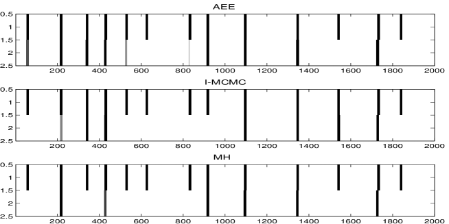
Figure 5: Results given by AEE, I-MCMC and a MH sampler

To highlight the major role of the equi-energy jumps, and the importance of the construction of the rings to make the acceptance probability of the jumps large enough, we compare AEE to I-MCMC, and to MH. The data are obtained with values of $p_{0},v_{0}$ and $v$ similar to those of [22]: $p_{0}=0.005$, $b_{1}=2$, $b_{2}=200$, $\iota_{j,i}=1$ for all $j$, $i$, and

$$v_{0}=\left(\begin{array}[]{cccc}0.1&0.7&0.1&0.1\\ 0.1&0.1&0.7&0.1\\ 0.1&0.1&0.1&0.7\\ 0.7&0.1&0.1&0.1\end{array}\right),\,v=\left(\begin{array}[]{cccccccccccc}0.5&0.6&0.2&0.4&0.1&0.3&0.6&0.1&0.4&0.4&0.3&0\\ 0&0.2&0&0.2&0.8&0.7&0&0.9&0&0&0.2&0.3\\ 0&0&0.8&0&0&0&0&0&0.3&0.5&0.4&0.1\\ 0.5&0.2&0&0.4&0.1&0&0.4&0&0.3&0.1&0.1&0.6\end{array}\right).$$

We sample a sequence $\mathsf{S}$ of length $L=2000$ and the size of the motif is $w=12$.

We now detail how the MH and the Metropolis-Hastings steps of AEE and I-MCMC are run. For the Metropolis-Hastings stage, the proposal distribution $p(A_{n},\tilde{A}_{n+1})$ is of the form

$$p(A_{n},\tilde{A}_{n+1})=q_{0}(\tilde{a}_{1}^{n+1})\ \prod_{j=1}^{L-1}q_{j}(\tilde{a}_{j}^{n+1},\tilde{a}_{j+1}^{n+1};A_{n})\;,$$

where we set $\tilde{A}_{n+1}=(\tilde{a}_{1}^{n+1},\cdots,\tilde{a}_{L}^{n+1})$. The proposed state $\tilde{A}_{n+1}$ of the Metropolis-Hastings step is then sampled element by element; the distributions are designed to be close to the previous model: $\tilde{a}_{j+1}^{n+1}$ equal to $\tilde{a}_{j}^{n+1}+1$ if $\tilde{a}_{j}^{n+1}\in\{1,\dots,w-1\}$, and else, $\tilde{a}_{j+1}^{n+1}$ is sampled under a Bernoulli distribution of parameter

$$\frac{\hat{p}_{0}\prod_{i=1}^{w}\hat{v}_{A_{n}}(s_{j+i-1},i)}{\hat{p}_{0}\prod_{i=1}^{w}\hat{v}_{A_{n}}(s_{j+i-1},i)+(1-\hat{p}_{0})\prod_{i=1}^{w-1}v_{0}(s_{j+i},s_{j+i+1})}\;;$$ (15)

the replacement constant $\hat{p}_{0}$ is fixed by the users and $\hat{v}_{A_{n}}$ is given by $\hat{v}_{A_{n}}(s,i)\propto c_{s,i}(A_{n})+c$ - where $c$ is a value fixed by the users. $q_{0}(\tilde{a}_{1}^{n+1})$ is the Bernoulli distribution with parameter (15). Finally, the candidate $\tilde{A}_{n+1}$ is accepted with probability

$$1\wedge\frac{\mathrm{P}(\tilde{A}_{n+1}|S)^{1/T_{k}}}{\mathrm{P}(A_{n}|S)^{1/T_{k}}}\frac{p(\tilde{A}_{n+1},A_{n})}{p(A_{n},\tilde{A}_{n+1})}\;.$$

Figure 5 displays the results obtained by AEE, I-MCMC and a MH sampler. Each subplot displays two horizontal lines with length equal to the length of the observed DNA sequence. The upper line represents the actual localization of the motifs, and the lower line represents in gray-scale the probability for each position to be part of a motif computed by one run of each algorithm after $2000$ iterations. For AEE and I-MCMC, we choose $\varepsilon=0.1$, $K=5$, $S=3$. The acceptance rate of the jump for AEE was about five times higher than for I-MCMC, which confirms the interest of the rings. As expected, AEE performs better than the other algorithms: there were $13$ actual motifs, and AEE retrieved $10$ motifs, whereas the I-MCMC and the MH retrieved respectively $7$ and $6$ motifs.

5 Conclusion

As illustrated by the numerical examples, the efficiency of EE depends upon the choice of the energy rings. The adaptation we proposed improves this efficiency since it makes the probability of accepting a jump more stable. It is known that adaptation can destroy the convergence of the samplers: we proved that AEE converges under quite general conditions on the adapted bounds and these general conditions can be used to prove the convergence of AEE when applied with other adaptation strategies [35]. It is also the first convergence result for an interacting MCMC algorithm including a selection mechanism. Our sketch of proof can be a basis for the proof of other interacting MCMC such as the SIMCMC algorithm of [13], the Non-Linear MCMC algorithms described in [3, Section 3] or the PTEEM algorithm of [10].

Appendix A Results on the transition kernels $P_{\theta}^{(k)}$

Define

$$G_{\theta}(x)\stackrel{{\scriptstyle\mathrm{def}}}{{=}}\int g_{\theta}(x,z)\theta(\mathrm{d}z)\;,\qquad\tilde{\theta}(x,\mathrm{d}y)\stackrel{{\scriptstyle\mathrm{def}}}{{=}}\frac{g_{\theta}(x,y)\theta(\mathrm{d}y)}{G_{\theta}(x)}\;.$$ (16)

A.1 Proof of Proposition  3.2

The case $k=1$ is a consequence of EE2 since $P_{\theta}^{(1)}=P^{(1)}$ for any $\theta$ so that $\pi_{\theta}^{(1)}\propto\pi^{\beta_{1}}$. We now consider the case $k\in\{2,\cdots,K\}$: in the proof below, for ease of notations we will write $P$, $P_{\theta}$, $W$, $\lambda,b$ and $\pi_{\theta}$ instead of $P^{(k)}$, $P_{\theta}^{(k)}$, $W_{k}$, $\lambda_{k},b_{k}$ and $\pi_{\theta}^{(k)}$.

(a) Let $m\geq 1$ and $\theta\in\Theta_{m}$. By definition of $g_{\theta}$ (see (2)) and of $\Theta_{m}$ (see (5)), $1/m\leq\int g_{\theta}(x,y)\theta(\mathrm{d}y)\leq S$. Moreover, by EE2b

$$P_{\theta}W(x)=(1-\varepsilon)PW(x)+\varepsilon K_{\theta}W(x)\leq(1-\varepsilon)(\lambda W(x)+b)+\varepsilon K_{\theta}W(x)\;.$$

We have by (3), (10) and (16)

$$K_{\theta}W(x) =W(x)+\int W(y)\alpha_{\theta}(x,y)\left(1-\frac{\pi^{\tau_{k}\beta_{k}}(y)}{\pi^{\tau_{k}\beta_{k}}(x)}\right)\tilde{\theta}(x,\mathrm{d}y)\;.$$

By (4),

$$K_{\theta}W(x)\leq W(x)+m\int_{\{y,\pi(y)\leq\pi(x)\}}W(y)\frac{\pi^{\beta_{k}-\beta_{k-1}}(y)}{\pi^{\beta_{k}-\beta_{k-1}}(x)}\left(1-\frac{\pi^{\tau_{k}\beta_{k}}(y)}{\pi^{\tau_{k}\beta_{k}}(x)}\right)g_{\theta}(x,y){\theta}(\mathrm{d}y)\;.$$

Defining $\psi$ by $\psi(\sigma)=\sigma/(\sigma+1)^{(\sigma+1)/\sigma}$ gives the upper bound $\sup_{z\in[0,1]}z(1-z^{\sigma})\leq\psi(\sigma)$. Hence, $K_{\theta}W(x)\leq W(x)+Sm\ \psi\left(\tau_{k}\beta_{k}/(\beta_{k}-\beta_{k-1})\right){\theta}(W)$. This yields $P_{\theta}W(x)\leq\tilde{\lambda}W(x)+\tilde{b}m\theta(W)$ with $\tilde{\lambda}=(1-\varepsilon)\lambda+\varepsilon<1$ and $\tilde{b}=\varepsilon S\ \psi\left(\tau_{k}\beta_{k}/(\beta_{k}-\beta_{k-1})\right)+(1-\varepsilon)b$. The minorization condition comes from the lower bound $P_{\theta}(x,A)\geq(1-\varepsilon)P(x,A)$.

(b) Let $m\geq 1$ and $\theta\in\Theta_{m}$. By EE2a, $P$ is $\varphi$-irreducible and so is $P_{\theta}$; $P_{\theta}$ possesses a $1$-small set and is thus aperiodic. In addition, $P_{\theta}W\leq(1+\tilde{\lambda})W/2+\tilde{b}\theta(W)\mathbf{1}_{\{W\leq c\}}$, with $c\stackrel{{\scriptstyle\mathrm{def}}}{{=}}2\tilde{b}m\ \theta(W)(1-\tilde{\lambda})^{-1}$ and $\{W\leq c\}$ is a $1$-small set for $P_{\theta}$. By [28, Chapter 15], $\pi_{\theta}$ exists and $\pi_{\theta}(W)\leq\tilde{b}m\theta(W)(1-\tilde{\lambda})^{-1}$.

A.2 Ergodic behavior

Lemma A.1.

Assume EE1a and EE2. Then for all $a\in(0,1)$, for all $m\geq 1$ and all $\theta\in\Theta_{m}$, there exist $C_{\theta}$ and $\rho_{\theta}\in(0,1)$ such that for all $x\in\mathbf{X}$ and any $j\geq 1$ and any $k\in\{1,\cdots,K\}$,

$$\|\left(P_{\theta}^{(k)}\right)^{j}(x,.)-\pi_{\theta}^{(k)}\|_{W_{k}^{a}}\leq C_{\theta}\ \rho_{\theta}^{j}\ W^{a}_{k}(x)\;.$$ (17)

Let $k\in\{1,\cdots,K-1\}$ and assume in addition that $\lim_{n\to\infty}\theta_{n}^{(k)}(W_{k})=\theta_{\star}^{(k)}(W_{k})$ w.p.1. Then for any positive integer $q$, on the set $\bigcap_{n\geq q}\{\theta_{n}\in\Theta_{m_{\star}}\}$

$$\limsup_{n}\rho_{\theta_{n}^{(k)}}<1,\limsup_{n}C_{\theta_{n}^{(k)}}<+\infty,\mathbb{P}-\text{a.s. }\;.$$ (18)

Proof.

The proof in the case $k=1$ is a consequence of EE2 and [28, Chapter 15] since $P_{\theta}^{(1)}=P^{(1)}$. Consider the case $k\geq 2$. Here again, the dependence upon $k$ is omitted: $P_{\theta},W,\theta_{n}$ denote $P_{\theta}^{(k)},W_{k}$ and $\theta_{n}^{(k)}$.

Proof of (17) Let $a\in(0,1)$ and set $V=W^{a}$. By the Jensen’s inequality and Proposition 3.2, there exists $\bar{\lambda}\in(0,1)$ and $\bar{b}$ such that for any $m\geq 1$ and any $\theta\in\Theta_{m}$,

$$P_{\theta}V\leq\bar{\lambda}V+\bar{b}\,m\,\theta(W)^{a}\;.$$

Let $m\geq 1$ and $\theta\in\Theta_{m}$. By [16, Lemma 2.3.], (17) holds and there exist constants $C,\gamma>0$ such that for any $\theta\in\Theta_{m}$,

$$C_{\theta}\vee(1-\rho_{\theta})^{-1}\leq C\left(\bar{b}\ m\theta(W)\vee\delta_{\theta}^{-1}\vee(1-\bar{\lambda})^{-1}\right)^{\gamma}\;,$$

where $\delta_{\theta}$ is the minorizing constant of $P_{\theta}$ on the set $\{x:W(x)\leq 2\bar{b}m\,\theta(W)\,(1-\bar{\lambda})^{-1}-1\}$.

Proof of (18) For all $\omega\in\bigcap_{n\geq q}\{\theta_{n}\in\Theta_{m_{\star}}\}$,

$$\limsup_{n}\{C_{\theta_{n}(\omega)}\vee(1-\rho_{\theta_{n}(\omega)})^{-1}\}\leq C\left(\bar{b}\,m\,\limsup_{n}\theta_{n}(W)\vee\limsup_{n}\delta_{\theta_{n}(\omega)}^{-1}\vee(1-\bar{\lambda})^{-1}\right)^{\gamma}\;.$$

Since $\limsup_{n}\theta_{n}(W)=\theta_{\star}(W)<\infty$ w.p.1, $\limsup_{n}\delta_{\theta_{n}(\omega)}^{-1}<\infty$ w.p.1. thus showing that on the set $\bigcap_{n\geq q}\{\theta_{n}\in\Theta_{m_{\star}}\}$, $\limsup_{n}\{C_{\theta_{n}(\omega)}\vee(1-\rho_{\theta_{n}(\omega)})^{-1}\}<\infty$. This implies (18). ∎

A.3 Moment conditions

Let $m_{\star}>0$. Define for any positive integer $q$ and any $k\in\{1,\cdots,K-1\}$,

$$A_{q,n}^{(k)}=\bigcap_{\ell\leq k}\bigcap_{q\leq j\leq n}\left\{\theta_{j}^{(\ell)}\in\Theta_{m_{\star}}\right\}\quad\text{if $q\leq n$,}\quad\textrm{and}\quad A_{q,n}^{(k)}=\Omega\quad\text{otherwise;}$$

by convention, $A_{q,n}^{(0)}=\Omega$ for any $q,n\geq 0$.

Lemma A.2.

Assume EE1a, EE2 and $\mathbb{E}\left[W_{k}(Y_{0}^{(k)})\right]<\infty$ for any $k\in\{1,\cdots,K\}$. Then for any $k\in\{1,\cdots,K\}$,

$$\sup_{j\geq 1}\mathbb{E}\left[W_{k}(Y_{j}^{(k)})\mathbf{1}_{A_{q,j-1}^{(k-1)}}\right]<\infty\;.$$ (19)

Proof.

The proof is by induction on $k$. The case $k=1$ is a consequence of EE2 since $P_{\theta}^{(1)}=P^{(1)}$. Assume the property holds for $k\in\{2,\cdots,K-1\}$. In this proof, $W_{k+1},P_{\theta}^{(k+1)},\theta_{n}^{(k)},Y^{(k)},Y^{(k+1)},P^{(k+1)}$, $K_{\theta}^{(k+1)}$ will be denoted by $W,P_{\theta},\theta_{n},Y,X,P,K_{\theta}$.

By (6) and Proposition 3.2 we obtain, for $j>q$

$$\mathbb{E}\left[W(X_{j})\mathbf{1}_{A_{q,j-1}^{(k)}}\right] \leq\mathbb{E}\left[P_{\theta_{j-1}}W(X_{j-1})\mathbf{1}_{A_{q,j-1}^{(k)}}\right]$$

$$\leq\tilde{\lambda}\mathbb{E}\left[W(X_{j-1})\mathbf{1}_{A_{q,j-2}^{(k)}}\right]+\tilde{b}\,m_{\star}\,\mathbb{E}\left[\theta_{j-1}(W)\mathbf{1}_{A_{q,j-1}^{(k-1)}}\right]$$

$$\leq\tilde{\lambda}\mathbb{E}\left[W(X_{j-1})\mathbf{1}_{A_{q,j-2}^{(k)}}\right]+\tilde{b}\,m_{\star}\,\sup_{l}\mathbb{E}\left[W(Y_{l})\mathbf{1}_{A_{q,l-1}^{(k-1)}}\right]\;.$$

Since $W_{k+1}\in\mathcal{L}_{W_{k}}$, the induction assumption implies that $\sup_{l}\mathbb{E}\left[W(Y_{l})\mathbf{1}_{A_{q,l-1}^{(k-1)}}\right]<\infty$. Iterating this inequality allows to write that for some constant $C^{\prime}$

$$\sup_{j\geq q}\mathbb{E}\left[W(X_{j})\mathbf{1}_{A_{q,j-1}^{(k)}}\right]\leq C^{\prime}\ \mathbb{E}\left[W(X_{q})\right]\;.$$

Finally, by definition of $P_{\theta_{j}}$, either $P_{\theta_{j}}=P$ if $\theta_{j}\notin\bigcup_{m}\Theta_{m}$, or $P_{\theta_{j}}=(1-\epsilon)P+\epsilon K_{\theta_{j}}$ otherwise; note that if $\theta_{j}\in\bigcup_{m}\Theta_{m}$ then $\theta_{j}\in\Theta_{1/j}$. Since both $P$ and $P_{\theta}$ for $\theta\in\bigcup_{m}\Theta_{m}$ satisfy a drift inequality (see EE2 and Proposition 3.2), $\mathbb{E}\left[W(X_{q})\right]<\infty$ by (6). ∎

Appendix B Proof of Theorem 3.3

• $(k)$ There exists $m_{\star}>0$ such that $\mathbb{P}\left(\bigcup_{q\geq 1}\bigcap_{n\geq q}\{\theta_{n}^{(k)}\in\Theta_{m_{\star}}\}\right)=1$.

• $(k)$ for any $a\in(0,1)$ and any continuous function $f\in\mathcal{L}_{W_{k}^{a}}$,

  $$\lim_{n\to\infty}\pi_{\theta_{n}^{(k-1)}}^{(k)}(f)=\theta_{\star}^{(k)}(f)\;.$$

• $(k)$ For all bounded continuous function $f$, $\lim_{n\to\infty}\mathbb{E}\left[f(Y_{n}^{(k)})\right]=\theta_{\star}^{(1)}(f)$.

• $(k)$ $\theta_{\star}^{(k)}(W_{k+1})<+\infty$, and for any $a\in(0,\frac{1+\Gamma}{2}\wedge 1)$ and any continuous function $f$ in $\mathcal{L}_{W_{k}^{a}}$, $\theta_{n}^{(k)}(f)\rightarrow\theta_{\star}^{(k)}(f)$ a.s.

By Proposition 3.1, the conditions RR3 and RR4 hold for $k=1$; RR2 also holds for $k=1$ since $\pi_{\theta}^{(1)}=\theta_{\star}^{(1)}$ for any $\theta$. We assume that for any $j\leq k$, for $k\in\{1,\cdots,K-1\}$, the conditions RR1($j-1$), RR2($j$), RR3($j$) and RR4($j$) hold. We prove that RR1($k$), RR2($k+1$), RR3($k+1$) and RR4($k+1$) hold. To make the notations easier, the superscript $k$ is dropped from the notations: the auxiliary process $Y^{(k)}$ will be denoted by $Y$, and the process $Y^{(k+1)}$ by $X$; $P^{(k+1)},W_{k+1},K_{\theta}^{(k+1)},P_{\theta}^{(k+1)},\alpha_{\theta}^{(k+1)},\pi_{\theta}^{(k+1)}$ and $\theta_{n}^{(k)},\theta_{\star}^{(k)}$ are resp. denoted by $P,W,K_{\theta},P_{\theta},\alpha_{\theta},\pi_{\theta}$ and $\theta_{n},\theta_{\star}$.

Finally, we define the V-variation of the two kernels $P_{\theta}$ and $P_{\theta^{\prime}}$ by:

$$D_{V}(\theta,\theta^{\prime})=\sup_{x\in\mathbf{X}}\left(\frac{\|P_{\theta}(x,.)-P_{\theta^{\prime}}(x,.)\|_{V}}{V(x)}\right)\;.$$

When $V=1$, we will simply write $D$.

B.1 Proof of RR1($k$)

The proof is prefaced with a preliminary lemma.

Lemma B.1.

For all $l\in\{1,\cdots,S-1\}$ and any $\theta,\theta^{\prime}$,

$$\sup_{x\in\mathbf{X}}\left|h_{\theta,l}(x)-h_{\theta^{\prime},l}(x)\right|\leq\frac{1}{r}\sup_{l\in\{1,\cdots,S-1\}}\left|\xi_{\theta,l}-\xi_{\theta^{\prime},l}\right|\;.$$

Proof.

Note that $|(1-a)_{+}-(1-b)_{+}|\leq|b-a|$. Therefore, for all $x\in\mathbf{X}$ :

$$|h_{\theta,l}(x)-h_{\theta^{\prime},l}(x)|\leq\frac{\left|d(\pi_{u}(x),H_{\theta,l})-d(\pi_{u}(x),H_{\theta^{\prime},l})\right|}{r}\;.$$

This concludes the proof. ∎

(Proof of RR1($k$)) We prove there exist an integer $m_{\star}\geq 1$ and a positive r.v. $N$ such that

$$\mathbb{P}(N<\infty)=1\;,\qquad\mathbb{P}\left(\bigcap_{n\geq N}\left\{\inf_{x}\int g_{\theta_{n}}(x,y)\theta_{n}(\mathrm{d}y)\geq 1/m_{\star}\right\}\right)=1\;.$$

To that goal, we prove that with probability $1$, for all $n$ large enough,

$$\inf_{x}\int g_{\theta_{n}}(x,y)\theta_{n}(\mathrm{d}y)\geq\inf_{\ell\in\{1,\cdots,S-1\}}\int h_{\theta_{\star},\ell}(y)\ \theta_{\star}(\mathrm{d}y)\;,$$ (20)

and use the assumption EE3a. For all $x$ and $\theta$, there exists a ring index $l_{x,\theta}\in\{1,\cdots,S\}$ such that $\pi_{u}(x)\in H_{\theta,l_{x,\theta}}$. Upon noting that $d(\pi_{u}(x),H_{\theta,\ell_{x,\theta}})=0$, it holds

$$\liminf_{n}\inf_{x}\int g_{\theta_{n}}(x,y)\theta_{n}(\mathrm{d}y)\geq\liminf_{n}\inf_{l\in\{1,\cdots,S\}}\int h_{\theta_{n},l}(y)\theta_{n}(\mathrm{d}y)\;.$$

We write

$$\int h_{\theta_{n},l}(y)\theta_{n}(\mathrm{d}y) \geq\int h_{\theta_{\star},l}(y)\theta_{n}(\mathrm{d}y)-\int\left|h_{\theta_{n},l}(y)-h_{\theta_{\star},l}(y)\right|\theta_{n}(\mathrm{d}y)$$

$$\geq\int h_{\theta_{\star},l}(y)\theta_{n}(\mathrm{d}y)-\sup_{y\in\mathbf{X}}\left|h_{\theta_{n},l}(y)-h_{\theta_{\star},l}(y)\right|\;.$$

By definition of $h_{\theta_{\star},\ell}$, $y\mapsto h_{\theta_{\star},l}(y)$ is continuous and bounded. Therefore, by RR4(k), Lemma B.1 and EE3b, the proof of (20) is concluded by

$$\liminf_{n}\int h_{\theta_{n},l}(y)\theta_{n}(\mathrm{d}y)>\int h_{\theta_{\star},l}(y)\theta_{\star}(\mathrm{d}y)\;.$$

B.2 Proof of RR2($k+1$)

First of all, observe that by definition of $\pi_{\theta}$ (see Proposition 3.2) and the expression of $P_{\theta}$, $\pi_{\theta_{\star}}\propto\pi^{\beta_{k+1}}$. We check the conditions of [16, Theorem 2.11]. By Proposition a it is sufficient to prove that for any $q\geq 1$, $\lim_{n\to\infty}|\pi_{\theta_{n}}(f)-\pi_{\theta_{\star}}(f)|\mathbf{1}_{\bigcap_{j\geq q}\{\theta_{j}\in\Theta_{m_{\star}}\}}=0$ w.p.1.

Case $f$ bounded

Lemma A.1 and RR4($k$) show that on the set $\bigcap_{j\geq q}\{\theta_{j}\in\Theta_{m_{\star}}\}$, $\limsup_{n}C_{\theta_{n}}<\infty$ and $\limsup_{n}(1-\rho_{\theta_{n}})^{-1}<\infty$ w.p.1. Equicontinuity of the class $\{P_{\theta}f,\theta\in\Theta_{m_{\star}}\}$, where $f$ is a bounded continuous function on $\mathbf{X}$, will follow from Lemmas B.2 to B.4. Finally, the weak convergence of the transition kernels is proved in Lemma B.5.

Case $f$ unbounded

Following the same lines as in the proof of [16, Theorem 3.5], it can be proved that the above discussion for $f$ bounded and Proposition 3.2(b) imply

$$\lim_{n\to\infty}\{\pi_{\theta_{n}}(f)-\pi_{\theta_{\star}}(f)\}\mathbf{1}_{\cap_{j\geq q}\{\theta_{j}\in\Theta_{m_{\star}}\}}=0$$

w.p.1. for any continuous function $f$ such that $|f|_{W^{a}_{k+1}}<\infty$.

Lemma B.2.

For all $\theta\in\bigcup_{m}\Theta_{m}$, and $x,x^{\prime}$, $\sup_{y}\left|g_{\theta}(x,y)-g_{\theta}(x^{\prime},y)\right|\leq\frac{S}{r}|\pi(x)-\pi(x^{\prime})|$.

Proof.

By (2),

$$|g_{\theta}(x,y)-g_{\theta}(x^{\prime},y)|\leq\sum_{l=1}^{S}|h_{\theta,l}(x)-h_{\theta,l}(x^{\prime})|h_{\theta,l}(y)\leq\sum_{l=1}^{S}|h_{\theta,l}(x)-h_{\theta,l}(x^{\prime})|\;.$$

The proof is completed since

$$|h_{\theta,l}(x)-h_{\theta,l}(x^{\prime})|\leq\frac{|d(\pi(x),H_{\theta,l})-d(\pi(x^{\prime}),H_{\theta,l})|}{r}\leq\frac{|\pi(x)-\pi(x^{\prime})|}{r}\;.$$

∎

Lemma B.3.

Assume EE1a. For all $m\geq 1$, there exists a constant $C_{m}$ such that for all $x,x^{\prime},y,y^{\prime}\in\mathbf{X}$ and $\theta\in\Theta_{m}$

$$\left|\alpha_{\theta}(x,y)-\alpha_{\theta}(x^{\prime},y)\right| \leq C_{m}\,\left[\left|\pi^{\beta_{k}-\beta_{k+1}}(x)-\pi^{\beta_{k}-\beta_{k+1}}(x^{\prime})\right|+\left|\pi(x)-\pi(x^{\prime})\right|\right]\;,$$ (21)

$$\left|\alpha_{\theta}(x,y)-\alpha_{\theta}(x,y^{\prime})\right| \leq C_{m}\left[\left|\pi^{\beta_{k}-\beta_{k+1}}(y)-\pi^{\beta_{k}-\beta_{k+1}}(y^{\prime})\right|+\left|\pi(y)-\pi(y^{\prime})\right|\right]\;.$$ (22)

Proof.

By definition of $\alpha_{\theta}$ (see (4)), $\alpha_{\theta}(x,y)-\alpha_{\theta}(x^{\prime},y)=\left(1\wedge a\right)-\left(1\wedge b\right)$, with

$$a=\frac{\pi^{\beta_{k+1}-\beta_{k}}(y)}{\pi^{\beta_{k+1}-\beta_{k}}(x)}\frac{\int g_{\theta}(x,z)\theta(\mathrm{d}z)}{\int g_{\theta}(y,z)\theta(\mathrm{d}z)}\quad\textrm{and}\quad b=\frac{\pi^{\beta_{k+1}-\beta_{k}}(y)}{\pi^{\beta_{k+1}-\beta_{k}}(x^{\prime})}\frac{\int g_{\theta}(x^{\prime},z)\theta(\mathrm{d}z)}{\int g_{\theta}(y,z)\theta(\mathrm{d}z)}\;.$$

Note that $|(1\wedge a)-(1\wedge b)|\leq|a-b|\left(\mathbf{1}_{a\leq 1}+\mathbf{1}_{b\leq 1,a>1}\right)$. By symmetry, we can assume that $b\leq 1$ and this implies

$$\frac{\pi^{\beta_{k+1}-\beta_{k}}(y)}{\pi^{\beta_{k+1}-\beta_{k}}(x^{\prime})}\leq\frac{\int g_{\theta}(y,z)\theta(\mathrm{d}z)}{\int g_{\theta}(x^{\prime},z)\theta(\mathrm{d}z)}\leq Sm\;,$$

since $g_{\theta}(x,y)\leq S$. Therefore,

$$|a-b|=\frac{\pi^{\beta_{k+1}-\beta_{k}}(y)}{\int g_{\theta}(y,z)\theta(\mathrm{d}z)}\left|\frac{\int g_{\theta}(x,z)\theta(\mathrm{d}z)}{\pi^{\beta_{k+1}-\beta_{k}}(x)}-\frac{\int g_{\theta}(x^{\prime},z)\theta(\mathrm{d}z)}{\pi^{\beta_{k+1}-\beta_{k}}(x^{\prime})}\right|\\ \leq Sm\left[\pi^{\beta_{k+1}-\beta_{k}}(y)\left|\pi^{\beta_{k}-\beta_{k+1}}(x)-\pi^{\beta_{k}-\beta_{k+1}}(x^{\prime})\right|+m\left|\int(g_{\theta}(x,z)-g_{\theta}(x^{\prime},z))\theta(\mathrm{d}z)\right|\right]\;.$$

The proof of (21) is concluded by Lemma B.2. The proof of (22) is on the same lines and omitted. ∎

Lemma B.4.

Assume EE1 and EE2a. For any $m\geq 1$ and for any continuous bounded function $f$, the class of functions $\{P_{\theta}f,\theta\in\Theta_{m}\}$ is equicontinuous.

Proof.

Let $f$ be a continuous function on $\mathbf{X}$, bounded by $1$. Let $m\geq 1$ and $\theta\in\Theta_{m}$. We have

$$P_{\theta}f(x)-P_{\theta}f(x^{\prime})= (1-\varepsilon)\left(Pf(x)-Pf(x^{\prime})\right)+\varepsilon\left(f(x)-f(x^{\prime})\right)\left(1-\int\alpha_{\theta}(x^{\prime},y)\tilde{\theta}(x,\mathrm{d}y)\right)$$

$$+\varepsilon\int\left(f(y)-f(x)\right)\left(\alpha_{\theta}(x,y)-\alpha_{\theta}(x^{\prime},y)\right)\tilde{\theta}(x,\mathrm{d}y)$$

$$+\varepsilon\int\alpha_{\theta}(x^{\prime},y)(f(y)-f(x^{\prime}))(\tilde{\theta}(x,\mathrm{d}y)-\tilde{\theta}(x^{\prime},\mathrm{d}y))\;,$$

where $\tilde{\theta}$ is given by (16). This yields to

$$\left|P_{\theta}f(x)-P_{\theta}f(x^{\prime})\right|\leq \left|Pf(x)-Pf(x^{\prime})\right|+\left|f(x)-f(x^{\prime})\right|$$

$$+2\sup_{y}\left|\alpha_{\theta}(x,y)-\alpha_{\theta}(x^{\prime},y)\right|+2\left\|\tilde{\theta}(x,.)-\tilde{\theta}(x^{\prime},.)\right\|_{\mathrm{TV}}\;.$$

We have

$$\|\tilde{\theta}(x,.)-\tilde{\theta}(x^{\prime},.)\|_{\mathrm{TV}} \leq\frac{1}{G_{\theta}(x)}\sup_{y}\left|g_{\theta}(x,y)-g_{\theta}(x^{\prime},y)\right|+\frac{S}{G_{\theta}(x)G_{\theta}(x^{\prime})}\left|G_{\theta}(x)-G_{\theta}(x^{\prime})\right|$$

$$\leq m\sup_{y}\left|g_{\theta}(x,y)-g_{\theta}(x^{\prime},y)\right|+Sm^{2}\sup_{y}\left|g_{\theta}(x,y)-g_{\theta}(x^{\prime},y)\right|\;,$$

where $G_{\theta}$ is given by (16). So Lemmas B.2 and B.3 imply that for all $m\geq 1$, there exists a constant $C_{m}$ such that for all $\theta\in\Theta_{m}$:

$$\left|P_{\theta}f(x)-P_{\theta}f(x^{\prime})\right|\leq \left|Pf(x)-Pf(x^{\prime})\right|+\left|f(x)-f(x^{\prime})\right|$$

$$+C_{m}\left(|\pi(x)-\pi(x^{\prime})|+|\pi^{\beta_{k}-\beta_{k+1}}(x)-\pi^{\beta_{k}-\beta_{k+1}}(x^{\prime})|\right)\;.$$ (23)

The proof is concluded since $P$ is Feller and $\pi$ is continuous. ∎

Lemma B.5.

Let $m\geq 1$. Assume EE1, EE3b and RR4(k). For all $x\in\mathbf{X}$, there exists a set $\Omega_{x}$ such that $\mathbb{P}(\Omega_{x})=1$ and for all $\omega\in\Omega_{x}$ and any bounded continuous function $f$

$$\lim_{n\to\infty}\left|P_{\theta_{n}(\omega)}f(x)-P_{\theta_{\star}}f(x)\right|\mathbf{1}_{\bigcap_{j}\{\theta_{j}\in\Theta_{m}\}}=0\;.$$

Proof.

Following the same lines as in the proof of [16, Proposition 3.3.], it is sufficient to prove that for any $x\in\mathbf{X}$ and any bounded continuous function $f$, $\lim_{n\to\infty}P_{\theta_{n}}(f)=P_{\theta_{\star}}(f)$ w.p.1 on the set $\bigcap_{j}\{\theta_{j}\in\Theta_{m}\}$. Let $f$ and $x$ be fixed. We write

$$P_{\theta}f(x)-P_{\theta^{\prime}}f(x)= \varepsilon\int\left(\alpha_{\theta}(x,y)-\alpha_{\theta^{\prime}}(x,y)\right)\left(f(y)-f(x)\right)\tilde{\theta}(x,\mathrm{d}y)$$

$$+\varepsilon\int\alpha_{\theta^{\prime}}(x,y)\left(f(y)-f(x)\right)\left(\tilde{\theta}(x,\mathrm{d}y)-\tilde{\theta^{\prime}}(x,\mathrm{d}y)\right)\;,$$ (24)

where $\tilde{\theta}$ is given by (16). Moreover,

$$\tilde{\theta}(x,\mathrm{d}y)-\tilde{\theta^{\prime}}(x,\mathrm{d}y) =\frac{g_{\theta}(x,y)\theta(\mathrm{d}y)-g_{\theta^{\prime}}(x,y)\theta^{\prime}(\mathrm{d}y)}{G_{\theta}(x)}+g_{\theta^{\prime}}(x,y)\theta^{\prime}(\mathrm{d}y)\,\frac{(G_{\theta^{\prime}}(x)-G_{\theta}(x))}{G_{\theta}(x)G_{\theta^{\prime}}(x)}\;.$$

This yields to

$$\varepsilon^{-1}\left(P_{\theta_{n}}f(x)-P_{\theta_{\star}}f(x)\right)=\int\left(\alpha_{\theta_{n}}(x,y)-\alpha_{\theta_{\star}}(x,y)\right)\ \left(f(y)-f(x)\right)\tilde{\theta}_{n}(x,\mathrm{d}y)\\ -\int\frac{g_{\theta_{\star}}(x,y)}{G_{\theta_{n}}(x)}F(x,y)\left(\theta_{\star}(\mathrm{d}y)-\theta_{n}(\mathrm{d}y)\right)\\ -\int F(x,y)\left((g_{\theta_{n}}(x,y)-g_{\theta_{\star}}(x,y))\frac{\theta_{n}(\mathrm{d}y)}{G_{\theta_{n}}(x)}+g_{\theta_{\star}}(x,y)\theta_{\star}(\mathrm{d}y)\,\frac{(G_{\theta_{\star}}(x)-G_{\theta_{n}}(x))}{G_{\theta_{n}}(x)G_{\theta_{\star}}(x)}\right)\;,$$

where $F(x,y)=\alpha_{\theta_{\star}}(x,y)\left(f(y)-f(x)\right)$. There exists a constant $C_{m}$ such that on the set $\bigcap_{n}\{\theta_{n}\in\Theta_{m}\}$, (see the proof of Lemma B.3 for similar upper bounds)

$$\left|\alpha_{\theta_{n}}(x,y)-\alpha_{\theta_{\star}}(x,y)\right|\leq C_{m}\,\left|\frac{G_{\theta_{n}}(x)}{G_{\theta_{n}}(y)}-\frac{G_{\theta_{\star}}(x)}{G_{\theta_{\star}}(y)}\right|\\ \leq m^{2}SC_{m}\,\left(\left|G_{\theta_{n}}(x)-G_{\theta_{\star}}(x)\right|+\left|G_{\theta_{n}}(y)-G_{\theta_{\star}}(y)\right|\right)$$

where $G_{\theta}(x)$ is defined by (16). We write by definition of the function $g_{\theta}$ (see (2))

$$\sup_{x}\left|G_{\theta_{n}}(x)-G_{\theta_{\star}}(x)\right|\leq\sup_{x,z}|g_{\theta_{n}}(x,z)-g_{\theta_{\star}}(x,z)|+\sup_{x}\left|\int g_{\theta_{\star}}(x,z)\theta_{n}(\mathrm{d}z)-\int g_{\theta_{\star}}(x,z)\theta_{\star}(\mathrm{d}z)\right|\\ \leq 2\sum_{l=1}^{S}\sup_{z}|h_{\theta_{n},l}(z)-h_{\theta_{\star},l}(z)|+\sum_{l=1}^{S}\left|\int h_{\theta_{\star},l}(z)\theta_{n}(\mathrm{d}z)-\int h_{\theta_{\star},l}(z)\theta_{\star}(\mathrm{d}z)\right|\;.$$

By Lemma B.1 and EE3b, the first term converges to zero w.p.1. Since $t\mapsto h_{\theta_{\star},l}(t)$ is continuous, RR4(k) implies that the second term tends to zero w.p.1. Therefore, on the set $\bigcap_{n}\{\theta_{n}\in\Theta_{m}\}$, $\sup_{x,y}\left|\alpha_{\theta_{n}}(x,y)-\alpha_{\theta_{\star}}(x,y)\right|$ converges to zero w.p.1, as well as $\sup_{x,y}|g_{\theta_{n}}(x,y)-g_{\theta_{\star}}(x,y)|$, and $\sup_{x}\left|G_{\theta_{n}}(x)-G_{\theta_{\star}}(x)\right|$ .

Note that by Lemma B.3, $y\mapsto F(x,y)$ is bounded and continuous. Therefore, following the same lines as above, it can be proved that under RR4(k) and EE3b, on the set $\bigcap_{n}\{\theta_{n}\in\Theta_{m}\}$, $\lim_{n\to\infty}|\int F(x,y)\theta_{n}(x,\mathrm{d}y)-\int F(x,y)\theta_{\star}(x,\mathrm{d}y)|$ =0 w.p.1 ∎

B.3 Proof of RR3(k+1)

We check the conditions of [16, Theorem 2.1]. Let $f$ be a bounded continuous function on $\mathbf{X}$. By RR2(k+1), $\lim_{n\to\infty}\pi_{\theta_{n}}(f)=\pi_{\theta_{\star}}(f)\propto\pi^{\beta_{k+1}}$ w.p.1. Let $\delta>0$. By Proposition a, there exists $q\geq 1$ such that $\mathbb{P}(\bigcap_{n\geq q}\{\theta_{n}\in\Theta_{m_{\star}}\})\geq 1-\delta$. Following the same lines as in the proof of [16, Theorem 3.4], it can be proved by using Lemmas A.1, B.1 and B.6 and the condition EE3c that $\lim_{n\to\infty}\mathbb{E}\left[\left(f(X_{n})-\pi_{\theta_{n}}(f)\right)\mathbf{1}_{\bigcap_{n\geq q}\{\theta_{n}\in\Theta_{m_{\star}}\}}\right]=0$. This concludes the proof.

Lemma B.6.

For all $m\geq 1$, there exists a constant $C_{m}$ such that for any $\theta,\theta^{\prime}\in\Theta_{m}$,

$$D(\theta,\theta^{\prime})\leq C_{m}\left(\|\theta-\theta^{\prime}\|_{\mathrm{TV}}+\sup_{l,x}\left|h_{\theta,l}(x)-h_{\theta^{\prime},l}(x)\right|\right)\;.$$

Proof.

By definition of $P_{\theta}$, for all function $f$ bounded by $1$, (B.2) holds. So

$$D(\theta,\theta^{\prime}) \leq 2\varepsilon\sup_{x,y}|\alpha_{\theta}(x,y)-\alpha_{\theta^{\prime}}(x,y)|$$

$$+2\varepsilon Sm^{2}\,\left(\sup_{x,y}|g_{\theta}(x,y)-g_{\theta^{\prime}}(x,y)|+\|\theta-\theta^{\prime}\|_{\mathrm{TV}}+\sup_{x}|G_{\theta^{\prime}}(x)-G_{\theta}(x)|\right)\;.$$

The term $|\alpha_{\theta}(x,y)-\alpha_{\theta^{\prime}}(x,y)|$ is equal to $|1\wedge a-1\wedge b|$ with

$$a=\frac{\pi^{\beta_{k+1}-\beta_{k}}(y)\int g_{\theta}(x,z)\theta(\mathrm{d}z)}{\pi^{\beta_{k+1}-\beta_{k}}(x)\int g_{\theta}(y,z)\theta(\mathrm{d}z)}\quad\textrm{and}\quad b=\frac{\pi^{\beta_{k+1}-\beta_{k}}(y)\int g_{\theta^{\prime}}(x,z)\theta^{\prime}(\mathrm{d}z)}{\pi^{\beta_{k+1}-\beta_{k}}(x)\int g_{\theta^{\prime}}(y,z)\theta^{\prime}(\mathrm{d}z)}\;.$$

Note that $|1\wedge a-1\wedge b|\leq|b-a|\left(\mathbf{1}_{\{b\leq 1,a>1\}}+\mathbf{1}_{a\leq 1}\right)$. Therefore, for all $\theta,\theta^{\prime}\in\Theta_{m}$,

$$\sup_{x,y}|\alpha_{\theta}(x,y)-\alpha_{\theta^{\prime}}(x,y)|\leq S^{2}m^{2}\ \left(\sup_{x,y}|g_{\theta}(x,y)-g_{\theta^{\prime}}(x,y)|+\|\theta-\theta^{\prime}\|_{\mathrm{TV}}\right)\;.$$

The term $|G_{\theta^{\prime}}(x)-G_{\theta}(x)|$ is upper bounded by

$$|G_{\theta^{\prime}}(x)-G_{\theta}(x)|\leq\sup_{x,y}|g_{\theta}(x,y)-g_{\theta^{\prime}}(x,y)|+S\|\theta-\theta^{\prime}\|_{\mathrm{TV}}\;.$$

Moreover,

$$\left|g_{\theta}(x,y)-g_{\theta^{\prime}}(x,y)\right|=\left|\sum_{l=1}^{S}[h_{\theta,l}(x)h_{\theta,l}(y)-h_{\theta^{\prime},l}(x)h_{\theta^{\prime},l}(y)]\right|\leq 2S\sup_{l,x}|h_{\theta,l}(x)-h_{\theta^{\prime},l}(x)|\;.$$

This concludes the proof. ∎

B.4 Proof of RR4($k+1$)

Let $a\in(0,\frac{1+\Gamma}{2}\wedge 1)$ and set $V=W^{a}$. We check the conditions of [16, Theorem 2.7]. By Proposition 3.2, condition A3 of [16] holds. By RR2($k+1$), $\lim_{n\to\infty}\pi_{\theta_{n}}(f)=\pi_{\theta_{\star}}(f)$ w.p.1 for any continuous function $f$ in $\mathcal{L}_{W^{a}}$. Condition A4 (resp. A5) of [16] is proved in Lemma B.7 (resp. Lemma B.8).

Lemma B.7.

Assume EE1, EE2, EE3, RR4(k), RR1(j) and $\mathbb{E}[W_{j}(Y_{0}^{(j)})]<\infty$ for all $j\leq k$. Then for any $a\in(0,\frac{1+\Gamma}{2}\wedge 1)$

$$\sum_{j\geq 1}j^{-1}(L_{\theta_{j}}\vee L_{\theta_{j-1}})^{6}D_{W^{a}}(\theta_{j},\theta_{j-1})W^{a}(X_{j})<\infty\ \qquad\mathbb{P}-\text{a.s.,}$$

where $L_{\theta}=C_{\theta}\vee(1-\rho_{\theta})^{-1}$.

Proof.

By RR1(j) for all $j\leq k$, it is sufficient to prove that for any positive integer $q$

$$\sum_{j\geq 1}j^{-1}(L_{\theta_{j}}\vee L_{\theta_{j-1}})^{6}D_{V}(\theta_{j},\theta_{j-1})V(X_{j})\ \mathbf{1}_{A_{q,j}^{(k)}}<\infty\qquad\mathbb{P}-\text{a.s.}$$

where $A_{q,j}^{(k)}$ is defined in Appendix A.3. Following the same lines as in the proof of Lemma A.2, it can be proved that $\sum_{j=1}^{q}j^{-1}(L_{\theta_{j}}\vee L_{\theta_{j-1}})^{6}D_{V}(\theta_{j},\theta_{j-1})V(X_{j})<\infty$ w.p.1.

By Lemma A.1 and RR4(k), on the set $\bigcap_{l\geq q}\{\theta_{l}\in\Theta_{m_{\star}}\}$, $\limsup_{n}L_{\theta_{n}}<\infty$ w.p.1. Therefore, we have to prove that $\sum_{j\geq q}j^{-1}D_{V}(\theta_{j},\theta_{j-1})V(X_{j})\mathbf{1}_{A_{q,j}^{(k)}}<\infty$ w.p.1. Following the same lines as in the proof of Lemma B.6, we obtain that on the set $A_{q,j}^{(k)}$, there exists a constant $C_{m}$ such that

$$D_{V}(\theta_{j},\theta_{j-1}) \leq C_{m}\left(\sup_{l}\left|\xi_{\theta_{j},l}-\xi_{\theta_{j-1},l}\right|+\|\theta_{j}-\theta_{j-1}\|_{\mathrm{TV}}\right)\left(\|\theta_{j}\|_{V}+\|\theta_{j-1}\|_{V}\right)$$

$$+C_{m}\ \|\theta_{j}-\theta_{j-1}\|_{V}\;.$$

Set $s,\gamma$, such that $s=1\vee(2a)<1+\gamma<1+\Gamma$. By EE3c, there exists a r.v. $Z$ finite w.p.1 such that $\mathbb{P}$-a.s.

$$|\xi_{\theta_{n},l}-\xi_{\theta_{n-1},l}|+\|\theta_{n}-\theta_{n-1}\|_{\mathrm{TV}}\leq Z\left(\frac{1}{n^{\gamma}}+\frac{1}{n}\right)\;.$$

Therefore, it holds

$$\mathcal{I}_{\gamma}\stackrel{{\scriptstyle\mathrm{def}}}{{=}}\mathbb{E}\left[\left(\sum_{j\geq q}j^{-1}\left(j^{-\gamma}+j^{-1}\right)\left(\|\theta_{j}\|_{V}+\|\theta_{j-1}\|_{V}\right)V(X_{j})\mathbf{1}_{A_{q,j}^{(k)}}\right)^{\frac{1}{s}}\right]\\ \leq\sum_{j\geq q}j^{-1/s}\left(j^{-\gamma/s}+j^{-1/s}\right)\mathbb{E}\left[\left(\|\theta_{j}\|_{V}+\|\theta_{j-1}\|_{V}\right)^{\frac{1}{s}}V^{\frac{1}{s}}(X_{j})\mathbf{1}_{A_{q,j}^{(k)}}\right]\;.$$

We have,

$$\mathcal{I}_{\gamma}\leq 2C(\gamma)\ \sup_{j}\mathbb{E}\left[\left(\|\theta_{j}\|_{V}\right)^{\frac{2}{s}}\mathbf{1}_{A_{q,j}^{(k)}}\right]^{1/2}\ \sup_{j}\mathbb{E}\left[V(X_{j})^{\frac{2}{s}}\mathbf{1}_{A_{q,j}^{(k)}}\right]^{1/2}\ \;,$$

where $C(\gamma)\stackrel{{\scriptstyle\mathrm{def}}}{{=}}\sum_{j\geq q}\left(j^{(-1-\gamma)/s}+j^{-2/s}\right)$ is finite since $2/s>1$ and $1+\gamma>s$. Since $V^{2/s}\leq W$, Lemma A.2 implies that $\sup_{j}\mathbb{E}\left[W(X_{j})\mathbf{1}_{A_{q,j}^{(k)}}\right]<\infty$. In addition, since $2/s>1$ we have, by Jensen’s inequality,

$$\mathbb{E}\left[\|\theta_{j}\|_{V}^{\frac{2}{s}}\mathbf{1}_{A_{q,j}^{(k)}}\right] \leq\mathbb{E}\left[\left(\frac{1}{j}\sum_{p=1}^{j}V(Y_{p})\right)^{\frac{2}{s}}\mathbf{1}_{A_{q,j}^{(k-1)}}\right]\leq\mathbb{E}\left[\frac{1}{j}\sum_{p=1}^{j}V^{\frac{2}{s}}(Y_{p})\mathbf{1}_{A_{q,j}^{(k-1)}}\right]$$

$$\leq\sup_{p}\mathbb{E}\left[W(Y_{p})\mathbf{1}_{A_{q,p-1}^{(k-1)}}\right]$$

which is finite under Lemma A.2. Similarly, we prove that $\sum_{j\geq q}j^{-1}\|\theta_{j}-\theta_{j-1}\|_{V}V(X_{j})\mathbf{1}_{A_{q,j}^{(k)}}<\infty$ w.p.1, upon noting that $\|\theta_{j}-\theta_{j-1}\|_{V}\leq j^{-1}(V(Y_{j})+\theta_{j-1}(V))$. ∎

Lemma B.8.

Assume EE1, EE2, EE3a-b, RR4(k), RR1(j) and $\mathbb{E}[W_{j}(Y_{0}^{(j)})]<\infty$ for all $j\leq k$. For any $a\in(0,1)$,

$$\sum_{j\geq 1}j^{-1/a}L_{\theta_{j}}^{2/a}\ P_{\theta_{j}}W(X_{j})<\infty\;,\qquad\mathbb{P}-\text{a.s.}$$

Proof.

By RR1(j) for all $j\leq k$, it is sufficient to prove that for any positive integer $q$

$$\sum_{j\geq 1}j^{-1/a}L_{\theta_{j}}^{2/a}\ P_{\theta_{j}}W(X_{j})\ \mathbf{1}_{A_{q,j}^{(k)}}<\infty\qquad\mathbb{P}-\text{a.s.}$$

where $A_{q,j}^{(k)}$ is defined in Appendix A.3. Let $q\geq 1$. By Lemma A.1, $\sup_{j}L_{\theta_{j}}\mathbf{1}_{A_{q,j}^{(k)}}<\infty$ w.p.1; and, as in the proof of Lemma A.2, it can be proved that $\sup_{j}\mathbb{E}\left[P_{\theta_{j}}W(X_{j})\mathbf{1}_{A_{q,j}^{(k)}}\right]<\infty$. The proof is concluded since $\sum_{k}k^{-1/a}<\infty$. ∎

B.5 Proof of Proposition 3.4

The proof uses a Hoeffding inequality for (non-stationary) Markov chains. The following result is proved in [15, section 5.2, theorem 17].

Proposition B.9.

Let $(Y_{k})_{k\in\mathbb{N}}$ be a Markov chain on $(\mathbf{X},\mathcal{X})$, with transition kernel $Q$ and initial distribution $\eta$. Assume $Q$ is $\overline{W}$-uniformly ergodic, and denote by $\theta_{\star}$ its unique invariant distribution. Then there exists a constant $K$ such that for any $t>0$ and for any bounded function $f:\mathbf{X}\rightarrow\mathbb{R}$

$$\mathbb{P}\left(\sum_{i=1}^{n}f(Y_{i})-n\theta_{\star}(f)\geq t\right)\leq K\eta(\overline{W})\exp\left[-\frac{1}{K}\left(\frac{t^{2}}{n|f|_{\infty}^{2}}\wedge\frac{t}{|f|_{\infty}}\right)\right]\;.$$

Lemma B.10.

Assume that there exists $\overline{W}$ such that $\{Y_{n},n\geq 0\}$ is a $\overline{W}$-uniformly ergodic Markov chain with initial distribution $\eta$ with $\eta(\overline{W})<\infty$. Let $l\in\{1,\cdots,S-1\}$ and $p_{l}\in(0,1)$; and set $\xi_{l}=F_{\theta_{\star}}^{-1}(p_{l})$. For all $\epsilon>0$ and any $n\geq 1$,

$$\mathbb{P}\left(|\xi_{\theta_{n},l}-\xi_{l}|>\epsilon\right)\leq 2K\eta(\overline{W})\exp\left(-\frac{n}{K}\left(\delta_{\epsilon}^{2}\wedge\delta_{\epsilon}\right)\right)\;,$$

where $\delta_{\epsilon}=min\left\{F_{\theta_{\star}}(\xi_{l}+\epsilon)-p_{l},p_{l}-F_{\theta_{\star}}(\xi_{l}-\epsilon)\right\}$.

Proof.

Let $\epsilon>0$. We write $\mathbb{P}\left(|\xi_{\theta_{n},l}-\xi_{l}|>\epsilon\right)\leq\mathbb{P}\left(\xi_{\theta_{n},l}\geq\xi_{l}+\epsilon\right)+\mathbb{P}\left(\xi_{\theta_{n},l}<\xi_{l}-\epsilon\right)$. Since $F_{\theta_{n}}(x)\leq t$ iff $x\leq F_{\theta_{n}}^{-1}(t)$,

$$\mathbb{P}\left(\xi_{\theta_{n},l}\geq\xi_{l}+\epsilon\right) =\mathbb{P}\left(F_{\theta_{n}}^{-1}(p_{l})\geq\xi_{l}+\epsilon\right)=\mathbb{P}\left(p_{l}\geq F_{\theta_{n}}(\xi_{l}+\epsilon)\right)$$

$$=\mathbb{P}\left(\sum_{k=1}^{n}\mathbf{1}_{\{\pi_{u}(Y_{k})>\xi_{l}+\epsilon\}}\geq n(1-p_{l})\right)\;.$$

Proposition B.9 is then applied with $f(x)=\mathbf{1}_{\{\pi_{u}(x)>\xi_{l}+\epsilon\}}$. As

$$\theta_{\star}(f)=\int\mathbf{1}_{\{\pi_{u}(x)>\xi_{l}+\epsilon\}}\theta_{\star}(dx)=1-F_{\theta_{\star}}(\xi_{l}+\epsilon)\;,$$

we obtain

$$\mathbb{P}\left(\xi_{\theta_{n},l}\geq\xi_{l}+\epsilon\right) =\mathbb{P}\left(\sum_{k=1}^{n}f(Y_{k})-n\theta_{\star}(f)\geq n\left(F_{\theta_{\star}}(\xi_{l}+\epsilon)-p_{l}\right)\right)$$

$$\leq K\eta(\overline{W})\exp\left(-\frac{n}{K}\left[\left(F_{\theta_{\star}}(\xi_{l}+\epsilon)-p_{l}\right)^{2}\wedge\left(F_{\theta_{\star}}(\xi_{l}+\epsilon)-p_{l}\right)\right]\right)\;.$$

for some constant $K$ independent of $n,l,\epsilon$. Similarly,

$$\mathbb{P}\left(\xi_{\theta_{n},l}<\xi_{l}-\epsilon\right)\leq K\eta(\overline{W})\,\exp\left(-\frac{n}{K}\left[\left(p_{l}-F_{\theta_{\star}}(\xi_{l}-\epsilon)\right)^{2}\wedge\left(p_{l}-F_{\theta_{\star}}(\xi_{l}-\epsilon)\right)\right]\right)\;,$$

which concludes the proof. ∎

Proof of Proposition 3.4 Let $f_{\theta_{\star}}=F^{\prime}_{\theta_{\star}}$ and $\epsilon_{n}$ be defined by

$$\epsilon_{n}=\frac{2\sqrt{2}}{f_{\theta_{\star}}(\xi_{l})}\sqrt{K}\sqrt{\frac{\log(n)}{n}}\;,$$

where $K$ is given by Lemma B.10. Note that under (i), $f_{\theta_{\star}}(\xi_{l})>0$ since $p_{l}\in(0,1)$. By (i), $F_{\theta_{\star}}$ is differentiable and we write when $n\to\infty$

$$F_{\theta_{\star}}(\xi_{l}+\epsilon_{n})-p_{l}=F_{\theta_{\star}}(\xi_{l}+\epsilon_{n})-F_{\theta_{\star}}(\xi_{l})=f_{\theta_{\star}}(\xi_{l})\epsilon_{n}+o(\epsilon_{n})\;.$$

Hence $F_{\theta_{\star}}(\xi_{l}+\epsilon_{n})-p_{l}\geq\sqrt{2K}\sqrt{\frac{\log(n)}{n}}$ for $n$ large enough. Similarly, $p_{l}-F_{\theta_{\star}}(\xi_{l}-\epsilon_{n})\geq\sqrt{2K}\sqrt{\frac{\log(n)}{n}}$ for $n$ large enough. So when $n$ is large enough, $nK^{-1}\left(\delta_{\epsilon_{n}}^{2}\wedge\delta_{\epsilon_{n}}\right)\geq 2\log(n)$ with $\delta_{\epsilon}$ defined in Lemma B.10. By Lemma B.10, for $n$ large enough, to

$$\mathbb{P}\left(|\xi_{\theta_{n},l}-\xi_{l}|>\epsilon_{n}\right)\leq\frac{2K\eta(\bar{W})}{n^{2}}\;.$$

As $\sum_{n=1}^{\infty}\mathbb{P}\left(|\xi_{\theta_{n},l}-\xi_{l}|>\epsilon_{n}\right)<\infty$, the Borel-Cantelli lemma yields $\limsup_{n}\epsilon_{n}^{-1}\left|\xi_{\theta_{n},l}-\xi_{l}\right|<\infty$ w.p.1. This concludes the proof.

References

- [1] C. Andrieu, A. Jasra, A. Doucet, and P. Del Moral. Non-linear Markov chain Monte Carlo. In Conference Oxford sur les méthodes de Monte Carlo séquentielles, volume 19 of ESAIM Proc., pages 79–84. 2007.
- [2] C. Andrieu, A. Jasra, A. Doucet, and P. Del Moral. A note on convergence of the Equi-Energy Sampler. Stoch. Anal. Appl., 26(2):298–312, 2008.
- [3] C. Andrieu, A. Jasra, A. Doucet, and P. Del Moral. On nonlinear Markov chain Monte Carlo. Bernoulli, 17(3):987–1014, 2011.
- [4] C. Andrieu and E. Moulines. On the ergodicity property of some adaptive MCMC algorithms. Ann. Appl. Probab., 16(3):1462–1505, 2006.
- [5] C. Andrieu and J. Thoms. A tutorial on adaptive MCMC. Stat. Comput., 18(4):343–373, 2008.
- [6] Y. Atchadé, G. Fort, E. Moulines, and P. Priouret. Adaptive Markov chain Monte Carlo: Theory and Methods, chapter 2, pages 33–53. Bayesian Time Series Models, Cambridge Univ. Press, 2011.
- [7] Y. F. Atchadé and J. S. Liu. Discussion of the “equi-energy sampler” by Kou, Zhou and Wong. Ann. Statist., 34:1620–1628, 2006.
- [8] Y. F. Atchadé, G. O. Roberts, and J. S. Rosenthal. Towards optimal scaling of Metropolis-coupled Markov chain Monte Carlo. Stat. Comput., 21(4):555–568, 2011.
- [9] Timothy L. Bailey and Charles Elkan. Fitting a Mixture Model By Expectation Maximization to Discover Motifs in Biopolymers. In Second International Conference on Intelligent Systems for Molecular Biology, 1994.
- [10] M. Baragatti, A. Grimaud, and D. Pommeret. Parallel tempering with equi-energy moves. Stat. Comput., pages 1–17, 2012.
- [11] B. Bercu, P. Del Moral, and A. Doucet. A Functional Central Limit Theorem for a class of Interacting Markov Chain Monte Carlo Methods. Electron. J. Probab., 14:2130–2155, 2009.
- [12] P. Billingsley. Convergence of Probability Measures. John Wiley & Sons, New York, 1968.
- [13] A. Brockwell, P. Del Moral, and A. Doucet. Sequentially interacting Markov chain Monte Carlo methods. Ann. Statist., 38(6):3387–3411, 2010.
- [14] P. Del Moral and Arnaud Doucet. Interacting Markov Chain Monte Carlo methods for solving nonlinear measure-valued equations. Ann. Appl. Probab., 20(2):593–639, 2010.
- [15] R. Douc, E. Moulines, J. Olsson, and R. VanHandel. Consistency of the maximum likelihood estimator for general hidden Markov models. Ann. Statist., 39(1):474–513, 2011.
- [16] G. Fort, E. Moulines, and P. Priouret. Convergence of adaptive and interacting Markov chain Monte Carlo algorithms. Ann. Statist., 39(6):3262–3289, 2012.
- [17] G. Fort, E. Moulines, P. Priouret, and P. Vandekerkhove. A simple variance inequality for U-statistics of a Markov chain with applications. Accepted in Stat. Probab. Lett., 2012.
- [18] C. J. Geyer. Markov chain Monte Carlo maximum likelihood. Computing Science and Statistics: Proc. 23rd Symposium on the Interface, Interface Foundation, Fairfax Station, VA, pages 156–163, 1991.
- [19] H. Haario, E. Saksman, and J. Tamminen. Adaptive proposal distribution for random walk Metropolis algorithm. Comput. Statist., 14:375–395, 1999.
- [20] W. K. Hastings. Monte Carlo sampling methods using Markov chains and their application. Biometrika, 57:97–109, 1970.
- [21] S. Jarner and E. Hansen. Geometric ergodicity of Metropolis algorithms. Stoch. Proc. Appl., 85(2):341–361, 2000.
- [22] S. C. Kou, Q. Zhou, and W. H. Wong. Equi-energy sampler with applications in statistical inference and statistical mechanics. Ann. Statist., 34(4):1581–1619, 2006.
- [23] C. E. Lawrence, S. F. Altschul, M. S. Boguski, J. S. Liu, A. F. Neuwald, and J. C. Wootton. Detecting subtle sequence signals: a Gibbs sampling strategy for multiple alignment. Science, 262:208–214, 1993.
- [24] Charles E. Lawrence and Andrew A. Reilly. An expectation maximization (EM) algorithm for the identification and characterization of common sites in unaligned biopolymer sequences. Proteins: Structure, Function, and Genetics, 7(1):41–51, 1990.
- [25] J. S. Liu, A. F. Neuwald, and C. E. Lawrence. Bayesian Models for Multiple Local Sequence Alignment and Gibbs Sampling Strategies. J. Am. Statist. Assoc., 90(432):1156–1170, 1995.
- [26] X. Liu, Douglas L. Brutlag, and Jun S. Liu. BioProspector: Discovering Conserved DNA Motifs in Upstream Regulatory Regions of Co-Expressed Genes. In Pacific Symposium on Biocomputing, pages 127–138, 2001.
- [27] N. Metropolis, A. W. Rosenbluth, M. N. Rosenbluth, A. H. Teller, and E. Teller. Equations of state calculations by fast computing machines. J. Chem. Phys., 21:1087–1092, 1953.
- [28] S. P. Meyn and R. L. Tweedie. Markov Chains and Stochastic Stability. Springer, London, 1993.
- [29] G. O. Roberts and J. S. Rosenthal. Coupling and ergodicity of adaptive Markov chain Monte Carlo algorithms. J. Appl. Probab., 44(2):458–475, 2007.
- [30] G.O. Roberts and R.L. Tweedie. Geometric convergence and central limit theorems for multidimensional Hastings and Metropolis algorithms. Biometrika, 83(1):95–110, 1996.
- [31] J. S. Rosenthal. MCMC Handbook, chapter Optimal Proposal Distributions and Adaptive MCMC. Chapman & Hall/CRC Press, 2009.
- [32] J.S. Rosenthal and D.B. Woodard. Convergence rate of Markov chain methods for genomic motif discovery. Under second review at Ann. Statist., 2012.
- [33] F. P. Roth, J. D. Hughes, P. W. Estep, and G. M. Church. Finding DNA regulatory motifs within unaligned noncoding sequences clustered by whole-genome mRNA quantitation. Nature biotechnology, 16(10):939–945, 1998.
- [34] Eero Saksman and Matti Vihola. On the ergodicity of the adaptive Metropolis algorithm on unbounded domains. Ann. Appl. Probab., 20(6):2178–2203, November 11 2010.
- [35] A. Schreck, G. Fort, A. Garivier, E. Moulines, and M. Vihola. Convergence of stochastic approximation with discontinuous dynamics. Work in progress, 2012.
- [36] G. D. Stormo and G. W. Hartzell. Identifying protein-binding sites from unaligned DNA fragments. In Proceedings of the National Academy of Sciences of the United States of America, volume 86, pages 1183–1187, February 1989.