Statistical thermodynamics of long straight rigid rods on triangular lattices: nematic order and adsorption thermodynamic functions

Abstract

The statistical thermodynamics of straight rigid rods of length $k$ on triangular lattices was developed on a generalization in the spirit of the lattice-gas model and the classical Guggenheim-DiMarzio approximation. In this scheme, the Helmholtz free energy and its derivatives were written in terms of the order parameter $\delta$, which characterizes the nematic phase occurring in the system at intermediate densities. Then, using the principle of minimum free energy with $\delta$ as a parameter, the main adsorption properties were calculated. Comparisons with Monte Carlo simulations and experimental data were performed in order to evaluate the reaches and limitations of the theoretical model.

UNSL] Departamento de Física, Instituto de Física Aplicada, Universidad Nacional de San Luis-CONICET, Chacabuco 917, D5700BWS San Luis, Argentina

1 1. Introduction

The adsorption of gases on solid surfaces is a topic of fundamental interest for various applications ^{1, 2}. From the theoretical point of view, the process can be described in terms of the lattice-gas model ^{3, 4, 5, 6, 7, 8}. A lattice gas is a system of $N$ molecules bound not more than one per site to a set of $M$ equivalent, distinguishable, and independent sites, and without interactions between bound molecules. Many studies have been carried out on the adsorption behavior of small molecules in such systems. However, the problem in which a 2D lattice contains isolated points (vacancies) as well as $k$-mers (particles occupying $k$ adjacent sites) has not been solved in closed form and still represents a major challenge in surface science.

A previous paper ⁹ was devoted to the study of long straight rigid rods adsorbed on square lattices. In Ref. [⁹], the Helmholtz free energy of the system and its derivatives were written in terms of the order parameter $\delta$, which characterizes the nematic phase occurring in the system at intermediate densities ^{10, 11}. Then, using the principle of minimum free energy with $\delta$ as a parameter, the main adsorption properties were calculated. Comparisons with Monte Carlo (MC) simulations revealed that the new thermodynamic description was significantly better than the existing theoretical models developed to treat the polymer adsorption problem.

In contrast to the statistic for the simple particles, where the arrangement of the adsorption sites in space is immaterial, the structure of lattice space plays such a fundamental role in determining the statistics of $k$-mers. Then, it is of interest and of value to inquire how a specific lattice structure influences the main thermodynamic properties of adsorbed polyatomics. In this sense, the aim of the present work is to extent the study in Ref. [⁹] to triangular lattices. The problem is not only of theoretical interest, but also has practical importance. A complete summary about adsorption on triangular lattices can be found in ^{12, 13, 14, 15} and references therein.

The rest of the paper is organized as follows. In Section 2, the theoretical formalism is presented. Section 3 is devoted to describe the Monte Carlo simulation scheme. The analysis of the results and discussion are given in Section 4. Finally, the conclusions are drawn in Section 5.

2 2. Model and theory

In this paper, the adsorption of straight rigid rods (or $k$-mers) on triangular lattices is considered. The adsorbate molecules are assumed to be composed by $k$ identical units in a linear array with constant bond length equal to the lattice constant $a$. The $k$-mers can only adsorb flat on the surface occupying $k$ lattice sites. The substrate is represented by a triangular lattice of $M=L\times L$ adsorption sites, with periodic boundary conditions. $N$ particles are adsorbed on the substrate with 3 possible orientations along the principal axis of the array [see $k$-mers marked with 1, 2 and 3 in Figure 1(a)]. The only interaction between different rods is hardcore exclusion: no site can be occupied by more than one $k$-mer unit. The surface coverage (or density) is defined as $\theta=kN/M$.

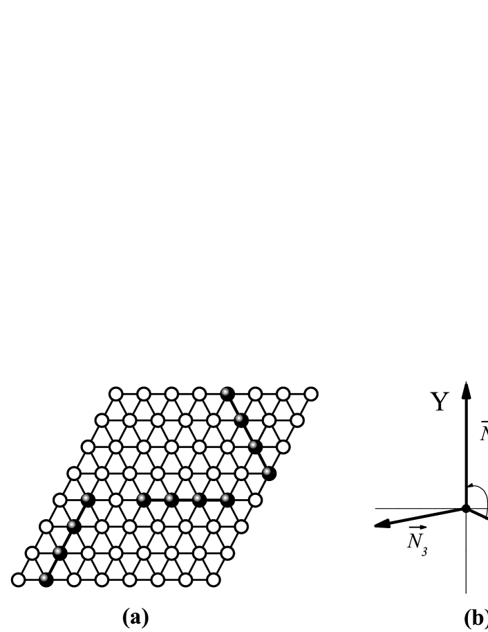
Figure 1: (a) Straight rigid rods adsorbed on triangular lattices. Solid circles (joined by thick lines) and empty circles represent tetramers ($k=4$) and empty sites, respectively. (b) Schematic representation of the set of vectors $\vec{N}_{1}$ , $\vec{N}_{2}$ , $\vec{N}_{3}$ for a triangular lattice

Let $N_{1}$, $N_{2}$ and $N_{3}$ be the number of rods oriented along directions 1, 2 and 3 on the surface, respectively. The total number of $k$-mers is $N=N_{1}+N_{2}+N_{3}$. According to DiMarzio’s lattice theory (DiMarzio 1961), the number of ways $\Omega(N_{0},N_{1},N_{2},N_{3})$ to pack the $N$ molecules such that $N_{i}$ of them lie in the direction $i$ and there are $N_{0}$ empty sites on the surface is given by

$$\begin{split}\Omega(M,N_{1},N_{2},N_{3})=&\frac{\prod_{j=1}^{3}\left[M-\left(k-1\right)N_{j}\right]!}{\left(N_{0}\right)!\prod_{i=1}^{3}\left(N_{i}\right)!\left(M!\right)^{2}},\end{split}$$ (1)

where $N_{0}=M-k\sum_{i}^{3}N_{i}$.

Since different $k$-mers do not interact with each other, all configurations of $N$ $k$-mers on $M$ sites are equally probable; henceforth, the canonical partition function $Q(M,N_{1},N_{2},N_{3},T)$ equals the total number of configurations, $\Omega(M,N_{1},N_{2},N_{3})$, times a Boltzmman factor including the total interaction energy between $k$-mers and lattice sites, $k\epsilon_{0}N$

$$Q(M,N_{1},N_{2},N_{3},T)=q(T)^{N}\Omega(M,N_{1},N_{2},N_{3})\exp\left(-{\beta k\epsilon_{o}N}\right),$$ (2)

where $q(T)$ is the partition function for a single adsorbed molecule, $\beta=1/k_{B}T$ (being $k_{B}$ the Boltzmann constant and $T$ the temperature) and $\epsilon_{o}$ is the interaction energy between every unit forming a $k$-mer and the substrate.

In the canonical ensemble the Helmholtz free energy $F(M,N_{1},N_{2},N_{3},T)$ relates to $\Omega(M,N_{1},N_{2},N_{3})$ through

$$\begin{split}\beta F(M,N_{1},N_{2},N_{3},T)=&-\ln Q(M,N_{1},N_{2},N_{3},T)\\ =&-N\ln q-\ln\Omega(M,N_{1},N_{2},N_{3})+\beta k\epsilon_{o}N.\end{split}$$ (3)

Then, the remaining thermodynamic functions can be obtained from the general differential form ¹⁶

$$dF=-SdT-\Pi dM+\mu dN,$$ (4)

where $S$, $\Pi$ and $\mu$ designate the entropy, spreading pressure and chemical potential respectively which by definition are,

$$S=-\left({\partial F\over\partial T}\right)_{M,N};\ \ \ \ \ \ \ \ \Pi=-\left({\partial F\over\partial M}\right)_{T,N};\ \ \ \ \ \ \ \ \ \mu=\left({\partial F\over\partial N}\right)_{T,M}.$$ (5)

2.1 Isotropic distribution of adsorbed $k$-mers

For the case of an isotropic distribution of the $k$-mers, i.e., $N_{1}=N_{2}=N_{3}=N/3$, 1 reduces to,

$$\Omega=\frac{\left\{\left[N_{0}+\left(2kN/3\right)+\left(N/3\right)\right]!\right\}^{3}}{N_{0}!\left[\left(N/3\right)!\right]^{3}\left(M!\right)^{2}}.$$ (6)

Applying the Stirling’s approximation to 6 and replacing in 3, the Helmholtz free energy per site $f=F/M$ can be written in terms of the intensive variables $\theta$ and $T$,

$$\begin{split}\beta f(\theta)=&-\left[3-\frac{(k-1)}{k}\theta\right]\ln\left[3-\frac{(k-1)}{k}\theta\right]+\frac{\theta}{k}\ln{\frac{\theta}{k}}+(1-\theta)\ln(1-\theta)\\ &-(\theta-3)\ln{3}+\beta\epsilon_{o}\theta-\frac{\theta}{k}\ln q(T).\end{split}$$ (7)

Then, the chemical potential and the entropy per site $s=S/M$ result

$$\begin{split}\beta\mu=&(k-1)\ln\left[1-\frac{(k-1)}{3k}\theta\right]+\ln\left(\frac{\theta}{3k}\right)-k\ln(1-\theta)-\ln K_{e}(T),\end{split}$$ (8)

and

$$\begin{split}\frac{s(\theta)}{k_{B}}=&\left[3-\frac{(k-1)}{k}\theta\right]\ln\left[3-\frac{(k-1)}{k}\theta\right]-\frac{\theta}{k}\ln{\frac{\theta}{k}}-(1-\theta)\ln(1-\theta)+(\theta-3)\ln{3}\\ &+\frac{\theta}{k}\left[\ln q(T)+T\frac{d\ln q(T)}{dT}\right],\end{split}$$ (9)

where $K_{e}(T)=q(T)\exp{(-\beta k\epsilon_{o}})$ is the equilibrium constant.

2.2 Anisotropic distribution of adsorbed k-mers

To introduce the effect of the orientational order in the GD theory, it is convenient to rewrite the configurational factor in 1 in terms of the nematic order parameter $\vec{\delta}$ ¹⁷,

$$\vec{\delta}=\frac{\sum_{i=1}^{m}\vec{N}_{i}}{\sum_{i=1}^{m}|\vec{N}_{i}|}.$$ (10)

$\vec{\delta}$ represents a general order parameter measuring the orientation of the $k$-mers on a lattice with $m$ directions and the set of vectors $\{\vec{N}_{1},\vec{N}_{2},\cdots,\vec{N}_{m}\}$ is characterized by the following properties: $(i)$ each vector is associated to one of the $m$ possible orientations (or directions) for a $k$-mer on the lattice; $(ii)$ the $\vec{N}_{i}$’s lie in a two-dimensional space (or are co-planar) and point radially outward from a given point $P$ which is defined as coordinate origin; $(iii)$ the angle between two consecutive vectors, $\vec{N}_{i}$ and $\vec{N}_{i+1}$, is equal to $2\pi/m$; and $(iv)$ the magnitude of $\vec{N}_{i}$ is equal to the number of $k$-mers aligned along the $i$-direction. Note that the $\vec{N}_{i}$’s have the same directions as the $q$ vectors in ¹⁷. These directions are not coincident with the allowed directions for the $k$-mers on the real lattice.

In the case of a triangular lattice, as studied here, $m=3$, the angle between $\vec{N}_{i}$ and $\vec{N}_{i+1}$ is $2\pi/3$ and 10 reduces to [see Figure 1(b)]:

$$\vec{\delta}=\frac{\vec{N}_{1}+\vec{N}_{2}+\vec{N}_{3}}{N_{1}+N_{2}+N_{3}}=\frac{\vec{N}_{1}+\vec{N}_{2}+\vec{N}_{3}}{N},$$ (11)

where $|\vec{N}_{i}|=N_{i}$ has been used for notational convenience.

$\vec{\delta}$ can be expressed in Cartesian form as $\vec{\delta}=\delta_{x}\hat{x}+\delta_{y}\hat{y}$, where

$$\delta_{x}=\frac{N_{1}-\frac{1}{2}N_{2}-\frac{1}{2}N_{3}}{N},$$ (12)

and

$$\delta_{y}=\frac{\frac{\sqrt{3}}{2}N_{2}-\frac{\sqrt{3}}{2}N_{3}}{N}.$$ (13)

In addition,

$$\begin{split}\theta=&\frac{kN}{M}=\frac{k\left(N_{1}+N_{2}+N_{3}\right)}{M}.\end{split}$$ (14)

Then, $N_{1}$, $N_{2}$ and $N_{3}$ can be written as a function of $\delta_{x}$, $\delta_{y}$ and $\theta$,

$$\begin{split}\frac{N_{1}}{M}=&\frac{\theta}{3k}\,\left(1+2\,\delta_{x}\right),\\ \frac{N_{2}}{M}=&\frac{\theta}{3k}\,\left(1-\delta_{x}+\sqrt{3}\,\delta_{y}\right),\\ \frac{N_{3}}{M}=&\frac{\theta}{3k}\,\left(1-\delta_{x}-\sqrt{3}\,\delta_{y}\right).\end{split}$$ (15)

Now, replacing 15 in the DiMarzio configurational factor 1 and using 3, the Helmholtz free energy per site can be written as,

$$\begin{split}\beta f(\theta,\delta_{x},\delta_{y})=&(1-\theta)\ln(1-\theta)\\ &-\left[1-\frac{(k-1)}{3k}\left(1+2\,\delta_{x}\right)\theta\right]\ln\left[1-\frac{(k-1)}{3k}\left(1+2\,\delta_{x}\right)\theta\right]\\ &-\left[1-\frac{(k-1)}{3k}\left(1-\delta_{x}+\sqrt{3}\,\delta_{y}\right)\theta\right]\ln\left[1-\frac{(k-1)}{3k}\left(1-\delta_{x}+\sqrt{3}\,\delta_{y}\right)\theta\right]\\ &-\left[1-\frac{(k-1)}{3k}\left(1-\delta_{x}-\sqrt{3}\,\delta_{y}\right)\theta\right]\ln\left[1-\frac{(k-1)}{3k}\left(1-\delta_{x}-\sqrt{3}\,\delta_{y}\right)\theta\right]\\ &+\frac{\left(1+2\,\delta_{x}\right)}{3k}\theta\ln\left[\frac{\left(1+2\,\delta_{x}\right)}{3k}\theta\right]\\ &+\frac{\left(1-\delta_{x}+\sqrt{3}\,\delta_{y}\right)}{3k}\theta\ln\left[\frac{\left(1-\delta_{x}+\sqrt{3}\,\delta_{y}\right)}{3k}\right]\\ &+\frac{\left(1-\delta_{x}-\sqrt{3}\,\delta_{y}\right)}{3k}\theta\ln\left[\frac{\left(1-\delta_{x}-\sqrt{3}\,\delta_{y}\right)}{3k}\right]+\beta\epsilon_{o}\theta-\frac{\theta}{k}\ln q(T).\\ \end{split}$$ (16)

Finally, from 5,

$$\begin{split}\beta\mu(\theta,\delta_{x},\delta_{y})=&\frac{(k-1)}{3}\left[1+2\left(\frac{\partial\delta_{x}}{\partial\theta}\theta+\delta_{x}\right)\right]\ln\left[1-\frac{(k-1)}{3k}\left(1+2\,\delta_{x}\right)\theta\right]\\ &+\frac{(k-1)}{3}\left[1+\left(\sqrt{3}\frac{\partial\delta_{y}}{\partial\theta}-\frac{\partial\delta_{x}}{\partial\theta}\right)\theta-\delta_{x}+\sqrt{3}\delta_{y}\right]\ln\left[1-\frac{(k-1)}{3k}\left(1-\delta_{x}+\sqrt{3}\,\delta_{y}\right)\theta\right]\\ &+\frac{(k-1)}{3}\left[1-\left(\sqrt{3}\frac{\partial\delta_{y}}{\partial\theta}+\frac{\partial\delta_{x}}{\partial\theta}\right)\theta-\delta_{x}-\sqrt{3}\delta_{y}\right]\ln\left[1-\frac{(k-1)}{3k}\left(1-\delta_{x}-\sqrt{3}\,\delta_{y}\right)\theta\right]\\ &+\frac{1}{3}\left[1+2\left(\frac{\partial\delta_{x}}{\partial\theta}\theta+\delta_{x}\right)\right]\ln\left[\frac{\left(1+2\,\delta_{x}\right)}{3k}\theta\right]\\ &+\frac{1}{3}\left[1+\left(\sqrt{3}\frac{\partial\delta_{y}}{\partial\theta}-\frac{\partial\delta_{x}}{\partial\theta}\right)\theta-\delta_{x}+\sqrt{3}\delta_{y}\right]\ln\left[\frac{\left(1-\delta_{x}+\sqrt{3}\,\delta_{y}\right)}{3k}\theta\right]\\ &+\frac{1}{3}\left[1-\left(\sqrt{3}\frac{\partial\delta_{y}}{\partial\theta}+\frac{\partial\delta_{x}}{\partial\theta}\right)\theta-\delta_{x}-\sqrt{3}\delta_{y}\right]\ln\left[\frac{\left(1-\delta_{x}-\sqrt{3}\,\delta_{y}\right)}{3k}\theta\right]\\ &-k\ln(1-\theta)-\ln K_{e}(T).\end{split}$$ (17)

and

$$\begin{split}\frac{s(\theta,\delta_{x},\delta_{y})}{k_{B}}=&\left[1-\frac{(k-1)}{3k}\left(1+2\,\delta_{x}\right)\theta\right]\ln\left[1-\frac{(k-1)}{3k}\left(1+2\,\delta_{x}\right)\theta\right]\\ &+\left[1-\frac{(k-1)}{3k}\left(1-\delta_{x}+\sqrt{3}\,\delta_{y}\right)\theta\right]\ln\left[1-\frac{(k-1)}{3k}\left(1-\delta_{x}+\sqrt{3}\,\delta_{y}\right)\theta\right]\\ &+\left[1-\frac{(k-1)}{3k}\left(1-\delta_{x}-\sqrt{3}\,\delta_{y}\right)\theta\right]\ln\left[1-\frac{(k-1)}{3k}\left(1-\delta_{x}-\sqrt{3}\,\delta_{y}\right)\theta\right]\\ &-\frac{\left(1+2\,\delta_{x}\right)}{3k}\theta\ln\left[\frac{\left(1+2\,\delta_{x}\right)}{3k}\theta\right]\\ &-\frac{\left(1-\delta_{x}+\sqrt{3}\,\delta_{y}\right)}{3k}\theta\ln\left[\frac{\left(1-\delta_{x}+\sqrt{3}\,\delta_{y}\right)}{3k}\theta\right]\\ &-\frac{\left(1-\delta_{x}-\sqrt{3}\,\delta_{y}\right)}{3k}\theta\ln\left[\frac{\left(1-\delta_{x}-\sqrt{3}\,\delta_{y}\right)}{3k}\theta\right]\\ &-(1-\theta)\ln(1-\theta)+\frac{\theta}{k}\left[\ln q(T)+T\frac{d\ln q(T)}{dT}\right],\end{split}$$ (18)

It is easy to see that, as $|\vec{\delta}|=0$, i.e. $\delta_{x}=0$ and $\delta_{y}=0$, the isotropic case is recovered and, consequently, LABEL:Fdelta,MU_delta reduce to 7-8. In general, the calculation of the adsorption isotherm and the configurational entropy of the adlayer requires the knowledge of an analytical expression for the dependence of the nematic order parameter on the coverage. For this purpose, a free-energy-minimization approach can be applied ⁹. The procedure is as follows:

• We choose $\delta_{y}=0$ and $\delta_{x}\neq 0$, this leaves $N_{2}$ and $N_{3}$ in an isotropic state, see 15. We can do this without losing any generality, since a pure nematic state is given by molecules aligned in one direction only ¹⁸.

• By differentiating 16 (with $\delta_{y}=0$) with respect to $\delta_{x}$ and setting the result equal to zero, the function $\delta(\theta)$ is obtained.

• $\delta(\theta)$ is introduced in LABEL:S_delta,MU_delta and thus the adsorption isotherm and the configurational entropy of the adlayer are obtained (without orientational restrictions).

The points (2) and (3) can be easily solved through a standard computing procedure; in our case, we used Maple software.

3 3. Monte Carlo simulation

In order to test the theory, an efficient hyper-parallel tempering Monte Carlo (HPTMC) simulation method ^{19, 20} has been used. The HPTMC method consists in generating a compound system of $R$ noninteracting replicas of the system under study. The $i$-th replica is associated with a chemical potential $\mu_{i}$. To determine the set of chemical potentials, $\{\mu_{i}\}$, the lowest chemical potential, $\mu_{1}$, is set in the isotropic phase where relaxation (correlation) time is expected to be very short and there exists only one minimum in the free energy space. On the other hand, the highest chemical potential, $\mu_{R}$, is set in the nematic phase whose properties we are interested in. Finally, the difference between two consecutive chemical potentials, $\mu_{i}$ and $\mu_{i+1}$ with $\mu_{i}<\mu_{i+1}$, is set as $\Delta\mu=\left(\mu_{1}-\mu_{R}\right)/(R-1)$ (equally spaced chemical potentials). The parameters used in the present study were as follows: $R=25$, $\mu_{1}=-10$ and $\mu_{R}=10$. With these values of the chemical potential, the corresponding values of the surface coverage varied from $\theta_{1}(\mu_{1})\approx 2\times 10^{-4}$ to $\theta_{R}(\mu_{R})\approx 0.99$ for $k=2$, and from $\theta_{1}(\mu_{1})\approx 2\times 10^{-3}$ to $\theta_{R}(\mu_{R})\approx 0.96$ for $k=10$.

Under these conditions, the algorithm to carry out the simulation process is built on the basis of two major subroutines: replica-update and replica-exchange.

Replica-update: The adsorption-desorption procedure is as follows: (1) One out of $R$ replicas is randomly selected. (2) A linear $k$-uple of nearest-neighbor sites, belonging to the replica selected in (1), is chosen at random. Then, if the $k$ sites are empty, an attempt is made to deposit a rod with probability $W=\min\left[1,\exp(\beta\mu)\right]$; if the $k$ sites are occupied by units belonging to the same $k$-mer, an attempt is made to desorb this $k$-mer with probability $W=\min\left[1,\exp(-\beta\mu)\right]$; and otherwise, the attempt is rejected. In addition, the displacement (diffusional relaxation) of adparticles to nearest-neighbor positions, by either jumps along the $k$-mer axis or reptation by rotation around the $k$-mer end, must be allowed in order to reach equilibrium in a reasonable time.

Replica-exchange: Exchange of two configurations $X_{i}$ and $X_{j}$, corresponding to the $i$-th and $j$-th replicas, respectively, is tried and accepted with probability $W=\min\left[1,\exp{(-\Delta)}\right]$. Where $\Delta$ in a nonthermal grand canonical ensemble is given by $[-\beta(\mu_{j}-\mu_{i})\,(N_{j}-N_{i})]$, and $N_{i}$ ($N_{j}$) represents the number of particles of the $i$-th ($j$-th) replica.

The complete simulation procedure is the following: (1) replica-update, (2) replica-exchange, and (3) repeat from step (1) $RM$ times. This is the elementary step in the simulation process or Monte Carlo step (MCs).

For each value of the chemical potential $\mu_{i}$, the equilibrium state can be well reproduced after discarding the first $r_{0}$ MCs. Then, a set of $r$ samples in thermal equilibrium is generated. The corresponding surface coverage $\theta_{i}(\mu_{i})$ is obtained through simple averages over the $r$ samples ($r$ MCs).

$$\theta_{i}(\mu_{i})=\frac{1}{r}\sum_{t=1}^{r}\theta\left[X_{i}(t)\right].$$ (19)

In the last equation, $X_{i}$ stands for the state of the $i$-th replica (at chemical potential $\mu_{i}$).

The configurational entropy $S$ of the adsorbate cannot be directly computed. To calculate entropy, various methods have been developed ²¹. Among them, the thermodynamic integration method is one of the most widely used and practically applicable. The method in the grand canonical ensemble relies upon integration of the chemical potential $\mu$ on coverage along a reversible path between an arbitrary reference state and the desired state of the system. This calculation also requires the knowledge of the total energy $U$ for each obtained coverage. Thus, for a system made of $N$ particles on $M$ lattice sites,

$$S(N,M,T)=S(N_{0},M,T)+{U(N,M,T)-U(N_{0},M,T)\over T}-{1\over T}\int_{N_{0}}^{N}{\mu dN^{\prime}}.$$ (20)

In the present case $U(N,M,T)=0$ and the determination of the reference state, $S(N_{0},M,T)$, is trivial because $S(N_{0},M,T)=0$ for $N_{0}=0$. Then, using intensive variables,

$${s(\theta,T)\over k_{B}}=-{1\over k_{B}T}\int_{0}^{\theta}{\frac{\mu}{k}~{}d\theta^{\prime}}.$$ (21)

4 4. Results

In this section, the main characteristics of the thermodynamic functions given in LABEL:S_delta,MU_delta will be analyzed in comparison with simulation results and the main theoretical models developed to treat the $k$-mers adsorption problem. Three theories have been considered: the first is the well-known FH approximation for straight rigid rods ^{22, 23}; the second is the GD approach for an isotropic distribution of admolecules ^{24, 25}; and the third is the recently developed SE model for the adsorption of polyatomics ^{26, 27}.

The equations of the GD adsorption isotherm and the GD configurational entropy for an isotropic distribution of adsorbed rods were given in LABEL:MUIS,SIS, respectively. The corresponding expressions in the FH and SE theories are as follows:

$$\beta\mu=\ln\left(\frac{\theta}{k}\right)-k\ln\left(1-\theta\right)-\ln\left(\frac{c}{2}\right)-\ln K_{e}(T)\ \ \ \ \ \ \ \ \ \ \ \ \ \ \ \ \ (k\geq 2)\ \ \ \ \ \ {\rm(FH)},$$ (22)

$$\begin{split}\beta\mu=&\ln\left(\frac{\theta}{k}\right)-k\ln\left(1-\theta\right)-\ln\left(\frac{c}{2}\right)+(1-\theta)(k-1)\ln\left[1-\frac{(k-1)}{k}\frac{2\theta}{c}\right]\\ &+\theta(k-1)\ln\left[1-\frac{(k-1)\theta}{k}\right]-\ln K_{e}(T)\ \ \ \ \ \ \ \ \ \ \ \ \ \ \ \ \ \ \ \ \ \ \ \ \ \ \ \ \ \ \ \ {\rm(SE)},\end{split}$$ (23)

$${s(\theta)\over k_{B}}=-{\theta\over k}\ln{\theta\over k}-\left(1-\theta\right)\ln\left(1-\theta\right)-{\theta\over k}\left[k-1-\ln\left(c\over 2\right)\right]+\frac{\theta}{k}\left[\ln q(T)+T\frac{d\ln q(T)}{dT}\right]\ \ \ \ \ \ \ \ \ {\rm(FH)},$$ (24)

and

$$\begin{split}{s(\theta)\over k_{B}}=&-{\theta\over k}\ln{\theta\over k}-\left(1-\theta\right)\ln\left(1-\theta\right)+\theta\left[{1\over 2}-{c\over 4}+{1\over k}\ln\left(c\over 2\right)\right]\\ &+{1\over 2}{k\over\left(k-1\right)}\left[1-{\left(k-1\right)^{2}\over k^{2}}\theta^{2}\right]\ln\left[1-{\left(k-1\right)\over k}\theta\right]\\ &-{c\over 4}\left[\theta+{k\left(c-4\right)+4\over 2\left(k-1\right)}\right]\left[1-{2\left(k-1\right)\over ck}\theta\right]\ln\left[1-{2\left(k-1\right)\over ck}\theta\right]\\ &+\frac{\theta}{k}\left[\ln q(T)+T\frac{d\ln q(T)}{dT}\right]\ \ \ \ \ \ \ {\rm(SE)}.\end{split}$$ (25)

The computational simulations have been developed for triangular $L\times L$ lattices with $L/k=20$ and periodic boundary conditions. With this size of the lattice we verified that finite size effects are negligible. As mentioned in Ref. [¹⁰], the relaxation time increases very quickly as the $k$-mer size increases. Consequently, MC simulations for large adsorbates are very time consuming and may produce artifacts related to non-accurate equilibrium states. In order to discard this possibility, equilibration times $r_{0}$ of the order O($10^{7}$ MCs) were used in this study.

An extensive comparison among the new adsorption isotherm [17, solid line], the simulation data (symbols), and the isotherm equations obtained from the analytical approaches depicted as GD [8, dashed line], FH [22, dashed and dotted line], and SE [23, dotted line] is shown in Figure 2: (a) $k=3$, (b) $k=8$ and (c) $k=10$. In the case of17, $\delta(\theta)$ was obtained by following the minimization procedure described at the end of Sec. II. In addition, $q(T)$ is set equal to one in the theoretical equations (vibrational and rotational degrees of freedom of the adsorbed molecules are not considered in the simulations).

Figure 2: Adsorption isotherms for rigid $k$-mers on a triangular lattice: (a) $k=3$, (b) $k=8$, and (c) $k=10$. Symbols represent the MC results, and lines correspond to different theoretical approaches as indicated in part (a). The corresponding order parameters, obtained from the minimization of the free energy in 16, are shown in the insets. (d) Average percent error in the chemical potential, $\epsilon_{\mu}$, as a function of $k$ for the different approximations studied in this contribution

In part (a), the behavior of the different approaches can be explained as follows. The new theory and GD agree very well with the simulation results for coverage values of up to $\theta\approx 0.8$; however, the disagreement between theoretical and simulation data increases for larger $\theta$ values. The coincidence between the new theory and GD results is due to the fact that, for small values of $k$ ($k<4$), the function $\delta(\theta)$ minimizing the free energy is $\delta(\theta)=0$ and, under this condition, 17 and 8 become identical. However, SE provides a good approximation with very small differences between simulation and theoretical results in all ranges of coverage.

Let us consider now the case of $k=8$ [Figure 2(b)]. The agreement between simulation and analytical data is very good for small values of coverage. However, as the surface coverage is increased, two different behaviors are observed. Although SE and the new theory provide good results, the classical FH and GD approximations fail to reproduce the simulation data. The differences between GD and the theory in 17 are associated with the behavior of the order parameter $\delta(\theta)$, which is shown in the inset of the figure. The functionality of $\delta$ with coverage is indicative of the existence of nematic order for $\theta>0.4$. Even though this result is not exact, the inclusion of $\delta(\theta)$ in 17 leads to an extremely good approximation of the adsorption isotherm.

The marked jump observed in the curve of the order parameter of a function of the coverage [see inset of Figure 2(b)] is indicative of the existence of a first-order phase transition in the adlayer. This behavior differs from that obtained for square lattices ⁹, where the continuous variation of the order parameter with density indicates clearly the presence of a second-order phase transition in the adsorbed layer. This point is extensively discussed in the recent paper by ²⁸.

Figure 2(c) is devoted to the analysis of large adsorbates ($k=10$, in the case of the figure). The results are very clear: (1) FH and GD predict a smaller $\theta$ than the simulation data over the entire range of coverage; (2) SE agrees very well with the simulation results for small and high values of the coverage; however, the disagreement turns out to be significantly large in a wide range of coverage ($0.3<\theta<0.9$); and (3) in the case of the new isotherm, the results are excellent and represent a significant advance with respect to the existing development of $k$-mer thermodynamics.

In order to compute the accuracy of each theory, the differences between theoretical and simulation data can be very easily rationalized by using the average percent error in the chemical potential $\varepsilon_{\mu}$, which is defined as,

$$\varepsilon_{\mu}=\frac{1}{N}\left(\sum_{\theta}\left|\frac{\mu_{\rm sim}-\mu_{\rm appr}}{\mu_{\rm sim}}\right|_{\theta}\right)\times 100\%,$$ (26)

where $\mu_{\rm sim}$ ($\mu_{\rm appr}$) represents the value of the chemical potential obtained by using the MC simulation (analytical approach). Each pair of values ($\mu_{\rm sim},\mu_{\rm appr}$) is obtained at fixed $\theta$. The sum runs over the $N$ points of the simulation adsorption isotherm (in this case, $N=25$ for all $k$).

The dependence of $\varepsilon_{\mu}$ on the $k$-mer size is shown in Figure 2(d) for the different theoretical approximations. Several conclusions can be drawn from the figure:

• In the FH and GD cases, $\varepsilon_{\mu}$ increases monotonically with increasing $k$ and the disagreement between MC and analytical data turns out to be very large (larger than 5$\%$) for $k\geq 5$ and $k\geq 6$, respectively.

• For the SE theory, there exists a range of $k$ ($2\leq k\leq 7$) where $\varepsilon_{\mu}$ remains almost constant around 1.5$\%$ and SE provides a very good fitting of the simulation data. However, for $k\geq 8$, the differences between simulation and theoretical data increase with $k$. This deviation is associated with the appearance of an I-N phase transition in the adlayer for $k>7$ ¹¹, which is not covered by the SE theory.

• The agreement between the equation reported here [17] and the simulation data is excellent over the whole coverage range. This result provides valuable insight into how the adsorption process takes place. Namely, for $k\geq 7$ and intermediate densities, it is more favorable for the rods to align spontaneously because the resulting loss of orientational entropy is compensated for by the gain of translational entropy.

• The comparison with previous results obtained for square lattices ⁹ reveals that, for a fixed value of $k$, (i) $\varepsilon_{\mu}$ increases with the connectivity for FH and GD theories, and (ii) in the case of SE approach and the new 17, $\varepsilon_{\mu}$ does not change significantly as the lattice geometry is varied.

The differences between the approaches analyzed in this work can be also appreciated by comparing the coverage dependence of the configurational entropy per site, which is presented in Figure 3 for the same cases studied in Figure 2. and triangular lattices, respectively. The overall behavior of $s(\theta)$ can be summarized as follows: for $\theta\rightarrow 0$ the entropy tends to zero. For low coverage, $s(\theta)$ is an increasing function of $\theta$, reaches a maximum at $\theta_{m}$, then decreases monotonically for $\theta>\theta_{m}$. The position of $\theta_{m}$ shifts to higher coverage as the $k$-mer size is increased. In the limit $\theta\rightarrow 1$ the entropy tends to a finite value, which is associated with the different ways to arrange the $k$-mers at full coverage. This value depends on $k$.

Figure 3: Same as Figure 2 for the configurational entropy of the adlayer

As in Figure 2, GD and FH appear as good approximations in the low-surface coverage region, but the disagreement turns out to be significantly large for $s(\theta_{m})$ and $s(\theta=1)$. On the other hand, SE shows a good agreement with MC simulations up to adsorbate sizes of $k\approx 8$. Finally, in the case of 18, the agreement is notable for all $\theta$, reproducing the MC results for $s(\theta_{m})$ and $s(\theta=1)$.

As in the case of the chemical potential, an average percent error ($\varepsilon_{s}$) was calculated for the difference between simulation and theoretical predictions. In this case,

$$\varepsilon_{s}=\frac{1}{N}\left(\sum_{\theta}\left|\frac{s_{\rm sim}-s_{\rm appr}}{s_{\rm sim}}\right|_{\theta}\right)\times 100\%,$$ (27)

where $s_{\rm sim}$ ($s_{\rm appr}$) represents the value of the configurational entropy per site obtained by using the MC simulation (analytical approach). As in 26, each pair of values ($s_{\rm sim},s_{\rm appr}$) is obtained at fixed $\theta$ and $N=25$.

The behavior of $\varepsilon_{s}$ is similar to that observed in Figure 2(d). However, two main differences can be marked: (1) FH performs better than GD for all values of $k$, and (2) the differences between SE and 26 are more notorious, with 26 being the most accurate for all cases.

Finally, analysis of experimental results have been carried out in order to test the applicability of the model proposed here. For this purpose, experimental adsorption isotherms of n-hexane in 5A zeolites, previously compiled by Silva and Rodrigues ²⁹, were analyzed in terms of 17. Given that the experimental data were reported in adsorbed amount (g/100 g adsorbed) as a function of pressure, the theoretical isotherms were rewritten in terms of the pressure $p$ and the adsorbed amount $Q$ as fitting quantities. Thus, assuming that the adsorbed phase is in equilibrium with a ideal gas phase, the pressure $p$ can be written as $p\propto\exp{(\beta\mu})$. In addition, $\theta=Q/Q_{max}$, where $Q_{max}$ represents the maximum adsorbed amount. This choice allows us a direct comparison of 17 with the results obtained in Ref. [²⁹].

Figure 4: Comparison between experimental and theoretical adsorption isotherms (adsorbed amount $Q$ vs pressure $p$) for $C_{6}H_{14}$ adsorbed in 5A zeolite. Symbols represent experimental data from Ref. [³²] and lines correspond to results from 17. The parameters used in the fitting procedure are listed in Table I

As is common in the literature ^{30, 31}, a “bead segment” chain model of the molecules was adopted, in which each methyl (bead) group occupies one adsorption site on the surface. Under this consideration, $k=6$ is set in the fitting data corresponding to $C_{6}$. In this scheme, a set of isotherms of n-hexane in 5A zeolites for different temperatures were correlated by using only one value of $Q_{max}$ and a temperature dependent $K_{e}(T)$ as adjustable parameters. The results are presented in Figure 4 and the fitting parameters are listed in Table I. A very good agreement between experimental and theoretical data is observed. In addition, the value obtained for the saturation adsorbed amount $Q_{max}=12.1$ is consistent with previous results reported in Refs. [^{30, 32}].

Temperature  (K)	$Q_{max}$  (g/100 $g_{ads}$)	$K_{e}$  (bar-1 )
473	12.1	0.109
523	12.1	0.402
573	12.1	1.597

Table 1: Table of parameters used in the fitting of Figure 4

In summary, the analysis presented in Figures 2-4 demonstrates that (1) explicitly considering the isotropic and nematic states occurring in the adlayer at different densities is crucial to understanding the adsorption process of rigid rods, and (2) LABEL:Fdelta,MU_delta provide a very good theoretical framework and compact equations to consistently interpret thermodynamic adsorption experiments of polyatomic species.

5 5. Conclusions

The adsorption process of straight rigid rods of length $k$ on triangular lattices has been studied via grand canonical Monte Carlo simulations, theory and analysis of experimental data. The proposed theoretical formalism, based on a generalization of the GD statistics, is capable of including the effects of the I-N phase transition occurring at intermediate densities on the thermodynamic functions of the system.

The results obtained (1) represent a significant qualitative advance with respect to former developments on $k$-mer thermodynamics; (2) demonstrates that explicitly considering the isotropic and nematic states occurring in the adlayer at different densities is crucial to understanding the adsorption process of rigid rods; and (3) provide a very good theoretical framework and compact equations to consistently interpret thermodynamic adsorption experiments of polyatomic species.

This work was supported in part by CONICET (Argentina) under project number PIP 112-200801-01332; Universidad Nacional de San Luis (Argentina) under project 322000 and the National Agency of Scientific and Technological Promotion (Argentina) under project PICT-2010-1466.

References

- 1 Crittenden B.; Thomas, W. J. Adsorption Technology and Design; Butterworth-Heinemann: Oxford, 1998.
- 2 Keller, J.; Staudt, R. Gas adsorption equilibria: experimental methods and adsorption isotherms; Springer: Boston, 2005.
- 3 Steele, W. A. The Interaction of Gases with Solid Surfaces; Pergamon Press: New York, 1974.
- 4 Dash, J. G. Films on Solid Surfaces; Academic Press: New York, 1975.
- 5 Dash, J. G.; Ruvalds, J. Phase Transitions in adsorbed Films; Plenum: New York, 1980.
- 6 Shina, S. K. Ordering in Two Dimensions; Elsevier: New York, 1980.
- 7 Binder, K.; Landau, D. P. Surf. Sci. 1976, 61, 577.
- 8 Patrykiejew, A.; Sokolowski, S.; Binder, K. Surface Science Reports 2000, 37, 207.
- 9 Matoz-Fernandez, D. A.; Linares, D. H.; Ramirez-Pastor, A. J. Langmuir 2011, 27, 2456.
- 10 Ghosh, A.; Dhar, D. Europhys. Lett. 2007, 78, 20003.
- 11 Matoz-Fernandez, D. A.; Linares, D. H.; Ramirez-Pastor, A. J. J. Chem. Phys. 2008, 128, 214902.
- 12 Phares, A. J.; GrumbineJr., D. W.; Wunderlich, F. J. Langmuir 2006, 22, 7646.
- 13 Phares, A. J.; GrumbineJr., D. W.; Wunderlich, F. J. Langmuir 2007, 23, 1928.
- 14 Phares, A. J.; GrumbineJr., D. W.; Wunderlich, F. J. Langmuir 2008, 24, 124.
- 15 Phares, A. J.; GrumbineJr., D. W.; Wunderlich, F. J. Langmuir 2009, 25, 944.
- 16 Hill, T. L. An Introduction to Statistical Thermodynamics; Addison Wesley Publishing Company: Reading, MA, 1960.
- 17 Wu, F. Y. Rev. Mod. Phys. 1982, 54, 235.
- 18 Oswald, P.; Pieranski, P. Nematic and Cholesteric Liquid Crystals: Concepts and Physical Properties Illustrated by Experiments; Taylor & Francis, CRC press: Boca Raton, 2005.
- 19 Yan, Q.; de Pablo, J. J. J. Chem. Phys 2000, 113, 1276.
- 20 Hukushima, K.; Nemoto, K. J. Phys. Soc. Jpn. 1996, 65, 1604.
- 21 Romá, F.; Ramirez-Pastor, A. J.; Riccardo, J. L. Langmuir 2000, 16, 9406.
- 22 Flory, P. J. J. Chem. Phys. 1942, 10, 51; Principles of Polymers Chemistry; Cornell University Press: Ithaca, N.Y., 1953.
- 23 Huggins, M. L. J. Phys. Chem. 1942, 46, 151; Ann. N. Y. Acad. Sci. 1942, 43, 1; J. Am. Chem. Soc. 1942, 64, 1712.
- 24 Guggenheim, E. A. Proc. R. Soc. London 1944, A183, 203.
- 25 DiMarzio, E. A. J. Phys. Chem. 1961, 35, 658.
- 26 Romá, F.; Riccardo J. L.; Ramirez-Pastor, A. J. Langmuir 2006, 22, 3192.
- 27 Riccardo, J. L.; Romá F.; Ramirez-Pastor, A. J. Int. J. Mod. Phys. B 2006, 20, 4709.
- 28 Dhar, D.; Rajesh, R.; Stilck, J. F. Phys. Rev E 2011, 84, 011140.
- 29 Silva, J. A. C.; Rodrigues, A. E. AIChE J. 1997, 43, 2524.
- 30 Romá, F.; Riccardo, J. L.; Ramirez-Pastor, A. J. Langmuir 2005, 21, 2454.
- 31 Romá, F.; Riccardo, J. L.; Ramirez-Pastor, A. J. Ind. Eng. Chem. Res. 2006, 45, 2046.
- 32 Silva, J. A. C.; Rodrigues, A. E. Ind. Eng. Chem. Res. 1999, 38, 2434.