On the statistics of area size in two-dimensional thick Voronoi Diagrams

Abstract

Cells of Voronoi diagrams in two dimensions are usually considered as having edges of zero width. However, this is not the case in several experimental situations in which the thickness of the edges of the cells is relatively large. In this paper, the concept of a thick Voronoi tessellation, that is with edges of non-zero width, is introduced and the statistics of cell areas, as thickness changes, are analyzed.

url]http://www.ph.unito.it/$\tilde{~{}}$zaninett

1 Introduction

Voronoi tessellations provide a powerful method for subdividing space in random partitions and have been used in a such diverse fields as statistical mechanics [1], quantum field theory [2], astrophysics [3], structure of matter [4], [5], [6], [7], biology [8] and medicine [9].

Algorithms to generate Voronoi diagrams can be found, among others, in [10], [11], [12] [13]; usually Voronoi partitions are obtained by considering a uniform spatial distribution of centers, so that the probability that there are $n$ points in a given domain of space obeys a Poisson distribution, of constant intensity $\lambda$ [12]. Non Poissonian distribution of seeds have been used in [14], in an astrophysical framework, and examples of area distribution for this case can be found in [15].

Usually, when generating Voronoi diagrams, the thickness of the edges is not taken into account, and, hence, its influence on the size of the cells is not considered. However, in nature, configurations occur that approximate Voronoi tessellations in which the width of edges is not negligible; examples can be found in the generation of diffraction patterns [16], in the compaction of granular matter [17] and crystallization of granular fluids [18], and in animal coat formation [19, 20].

In the next section probability distribution used to fit areas of $2D$ Poissonian Voronoi tessellation will be briefly reviewed; next the statistics of Poissonian thick Voronoi diagrams, that is with an edge of non-zero width, will be studied in the two-dimensional case and, in particular, the dependence of the mean and variance of the area distribution on the thickness of edges will be analyzed. Furthermore, a probability density function will be considered, adapted from that proposed in [21], to fit histograms of cell areas.

2 Probability distributions

Consider a $2D$ Poisson Voronoi Diagram (PVD for short) and let $a_{0}$ be the area of its cells.

No exact solution is known for the distribution of 2D Voronoi cells, however there exist several PDF, based of the Gamma distribution, that provide an approximate solution, with different degrees of ”goodness”: the most general way is via a $3$ parameter generalized Gamma distribution

$$G(x;a,b,c)=\frac{a{b}^{{\frac{c}{a}}}{x}^{c-1}{{\rm e}^{-b{x}^{a}}}}{\Gamma\left({\frac{c}{a}}\right)}\quad.$$ (1)

[22], [13]; here $x=a_{0}/\langle a_{0}\rangle$, where $\langle a_{0}\rangle$ is the area average. The previous PDF can be simplified inserting $a=1$ and the following $2$ parameters Gamma PDF is obtained

$$g(x;b,c)=\frac{{b}^{c}{x}^{c-1}{{\rm e}^{-bx}}}{\Gamma\left(c\right)}\quad,$$ (2)

[11, 23].

Note that the most recent numerical estimates of the parameters $c$ and $b$, in the $2D$ case, show that they are very close, namely $b$=3.52418 and $c$= 3.52440 [23]. This suggests the use of a one-parameter Gamma distribution,

$$p(x;c)=\frac{c^{c}}{\Gamma(c)}x^{c-1}\exp(-cx)\quad;$$ (3)

such a distribution has been used by Kiang in his seminal work on Voronoi diagrams [24]. Note, however, that in [24] it is has been assumed $c=2d$ where $d$ is just the dimensionality of the cells, so in the present case case $c=4$.

Finally in [21], a simpler distribution has been proposed with no free parameters, that can be obtained from (3) by setting $c=(3d+1)/2$, that is $c=3.5$ in $2D$:

$$f(x;d)={C}x^{\frac{3d-1}{2}}\exp{(-(3d+1)x)}\quad,$$ (4)

where

$$C=\frac{\left[\frac{3d+1}{2}\right]^{(3d+1)/2}}{\Gamma\left(\frac{3d+1}{2}\right)}$$ (5)

A detailed comparison between $f(x;d)$ and $G(x;a,b,c)$ can be found in [21]. The usefulness of these distributions in physical problems is determined by the trade off between the accuracy with which they fit the data and their complexity. We have computed $\delta=|f(x;d)-g(x;b,c)|$ the absolute value of the difference between $f(x;d)$ and $g(x;b,c)$, for the $2D$ and the resulting plot is shown in Fig. 1: the maximum value of $\delta$ is $0.0037$. Obviously, the PDF $g$ can give a better fit of the data, however $f$ is simpler and we think that, at least for the purposes of this note, provides a good enough approximation.

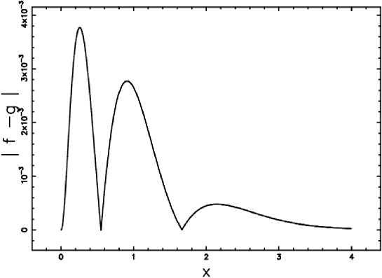
Figure 1: The absolute value of the difference between $f(x;d)$ and $g(x;b,c)$ as a function of $x$ when $d=2$, $b$=3.52418 and $c$= 3.52440.

For future reference we give here the variance and mode of (4) which are, respectively,

$$\sigma^{2}=\frac{2}{3d+1}$$ (6)

and

$$a_{m}=\frac{3d-1}{3d+1}\quad.$$ (7)

3 Two-dimensional thick Voronoi diagrams

Let $s$ be the thickness of edges of 2D cells in a Voronoi tessellation, denote with $a(s)$ the cells area and with $a_{0}$ the area when $s=0$.

The analysis of area size as a function of $s$ can be made independent of the area $A$ of the $2D$ domain $\mathcal{A}$ in which the Voronoi polygons are generated, by introducing a dimensionless parameter

$$\rho=\frac{s}{\langle a_{0}\rangle^{1/2}}=\frac{s}{\left(\frac{A}{n}\right)^{1/2}}\quad.$$ (8)

where $n$ is the number of seeds of the diagram.

An example of thick Voronoi diagrams, with $\rho=0.2$, is presented in Fig. 2 where, for illustrative purposes, just $n=150$ centers have been used; all simulations presented in the following have been carried out with $n=4\cdot 10^{4}$ centers.

Simulations were run on a LINUX -$2.66$GHz processor: Poisson Voronoi tessellation were generated by sampling independently the coordinates along $X$ and $Y$ axes from a uniform distribution by means of the subroutine RAN2 described in [25]. In order to minimize boundary effects introduced by cells crossing the boundary of the domain $\mathcal{A}$, a square $\mathcal{B}$ is defined larger by a factor $1.5$ and containing $\mathcal{A}$. The seeds are placed in the whole $\mathcal{B}$ domain; furthermore only cells that do not cross the boundary of $\mathcal{A}$ are considered, see Figure 2.

Further information on the code used here can be found in [26]. The CPU time running time was $1.42$ s for a seed.

It is obvious that increasing values of $\rho$ make more likely the occurrence of cells completely covered by edges and indeed, from Fig. 2, it can be seen that some of the smallest cells are completely covered. Moreover it is also apparent for $\rho=0.2$ a relatively large area of the cell is occupied by edges and this is confirmed by the results presented in the sequel. We have then restricted our analysis to $0\leq\rho\leq 0.2$.

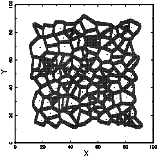
Figure 2: Thick Voronoi diagrams in 2D with $\rho=0.2$. The selected region comprises 150 random seeds marked by a point.Here, for simplicity $\langle a_{0}\rangle=1$.

In general the area $a$ can be considered to be obtained from $a_{0}=a(0)$ by the action of a mapping $K$, so that $a(\rho)=K(a_{0},\rho)$ rescales the cell size. Then $K$ can be seen as a nonlinear scaling operator and can be given in a form akin to that used for the group of scaling [27], namely

$$a(\rho)=k(a_{0},\rho)a_{0}.$$ (9)

Note that $k$ is a decreasing function of $a_{0}$, in that large cells are relatively less affected than small ones by the occurrence of an edge of width $s$.

Since cells are irregular polygons it is difficult to compute an explicit form of $a$ and $k$ since it depends on the shape of the cell, however some general properties are readily apparent, which suffice for our purposes. The area $a$ can not contain powers of $s$, and hence of $\rho$, larger than $2$, for reasons of dimensional consistency, and that holds for $k$ too (compare Eqs. (9)); it is also obvious that

$$k(a_{0},0)=1,\qquad dk(a_{0},\rho)/d\rho|_{\rho=0}<0.$$ (10)

Then $k$ can be written as

$$k(a_{0},\rho)=1-h(a_{0})\rho+\frac{1}{2}g(a_{0})\rho^{2},$$ (11)

where

$$h(a_{0})=\mid dk(a_{0},\rho)/d\rho\mid_{\rho=0}\mid,\qquad g(a_{0})=d^{2}k(a_{0},\rho)/d\rho^{2}\mid_{\rho=0},$$

and the area $a(\rho)$ is

$$a(\rho)=a_{0}\left(1-h(a_{0})\rho+\frac{1}{2}g(a_{0})\rho^{2}\right),$$ (12)

with the understanding that $a(\rho)$ is set to $0$ if Eq.(12) yields a value less then $0$.

Since $\rho$ is small, only the linear term in (11) needs to be considered, then

$$a(\rho)=a_{0}\left(1-h(a_{0})\rho+\frac{1}{2}g(a_{0})\rho^{2}\right)\approx a_{0}-a_{0}h(a_{0})\rho,$$ (13)

from which

$$\langle a(\rho)\rangle\approx\langle a_{0}\rangle-\langle a_{0}h(a_{0})\rangle\rho.$$ (14)

A linear decrease of the average area is also the outcome of simulations, as shown in Fig. 3 where a comparison with a linear fit is presented: values of $\langle a_{0}\rangle$ and $\langle a_{0}h(a_{0})\rangle$ have been computed by standard fitting procedures (least squares method) and are reported in Table 1.

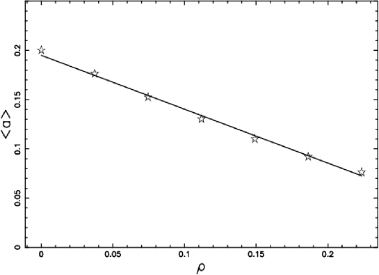
Figure 3: Area average versus thickness. The stars represent the results of the simulations and the full line is given by Eq. (14).

Table 1: Coefficients of the linear fit.

$$\begin{array}[]{llll}\hline\cr\langle a_{0}\rangle&\langle h(a_{0})a_{0}\rangle&\sigma^{2}_{a_{0}}&C\\ \vskip 3.0pt plus 1.0pt minus 1.0pt\cr\hline\cr\vskip 3.0pt plus 1.0pt minus 1.0pt\cr 0.19&0.55&0.01&0.016\\ \hline\cr\hline\cr\end{array}$$

It should be observed that the area decreases quite sharply even for values of $\rho$ which allow the linear approximation of Eq. (13); in particular for $\rho=0.2$, the average area is $\langle a(\rho)\rangle\approx 0.5\langle a_{0}\rangle$. The trend is linear up to $\rho=0.25$ approximately, for this value $\langle a(\rho)\rangle\approx 0.3\langle a_{0}\rangle$. For illustrative purposes Fig. 4 shows the trend of $\langle a(\rho)\rangle$ in the interval $0\leq\rho\leq 0.5$, fitted with the equation obtained by averaging the terms of Eq. (12), that is

$$\langle a(\rho)\rangle=\langle a_{0}\rangle-\langle a_{0}h(a_{0})\rangle\rho+\frac{1}{2}\langle a_{0}g(a_{0})\rangle\rho^{2}\quad.$$ (15)

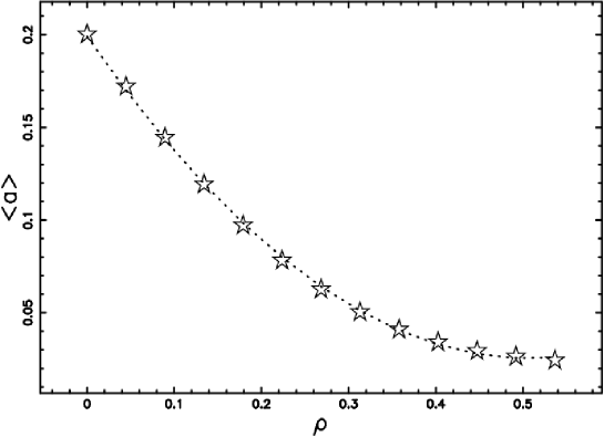
Figure 4: Area average versus thickness. The stars represent the results of the simulations and the full line Eq. (15) with $\langle a=0.2\rangle$ , $\langle h(a_{0})a_{0}\rangle=0.68$ and ${1}/{2}\langle a_{0}g(a_{0})\rangle=0.67$.

The variance $\sigma^{2}_{a}$ can then be calculated:

$$\sigma^{2}_{a}=\left<(a-\left<a\right>)^{2}\right>=\left<[(a_{0}-a_{0}h(a_{0})\rho)-\langle(a_{0}-a_{0}h(a_{0}))\rangle\rho]^{2}\right>,$$ (16)

from which it is straightforward to obtain:

$$\sigma^{2}_{a} = \left<(a_{0}-\langle a_{0}\rangle)^{2}\right>-2\left<(h(a_{0})a_{0}-\langle h(a_{0})a_{0}\rangle)(a_{0}-\langle a_{0}\rangle)\right>\rho$$ (17)

$$+ \left<(h(a_{0})a_{0}-\langle h(a_{0})a_{0}\rangle)^{2}\right>\rho^{2},$$

and, by making use again of the linear approximation,

$$\sigma^{2}_{a}\approx\left<(a_{0}-\langle a_{0}\rangle)^{2}\right>-2\rho\left<(h(a_{0})a_{0}-\langle h(a_{0})a_{0}\rangle)(a_{0}-\langle a_{0}\rangle)\right>.$$ (18)

Set

$$\left<(h(a_{0})a_{0}-\langle h(a_{0})a_{0}\rangle)(a_{0}-\langle a_{0}\rangle)\right>=C(h(a_{0})a_{0},a_{0}),$$

then Eq.(18) can be written as

$$\sigma^{2}_{a}\approx\sigma^{2}_{a_{0}}-2C(h(a_{0})a_{0},a_{0})\rho.$$ (19)

Now $C(h(a_{0})a_{0},a_{0})>0$, because it is the covariance of $h(a_{0})a_{0}$ with $a_{0}$ and, by definition, both $a_{0}$ and $h(a_{0})$ are positive; therefore, if the approximation of Eq. (18) holds, $\sigma^{2}_{a}$ must fall off linearly. Comparison between simulations and the results of Eq. (19) are shown in Fig. 5 and it is clear from the figure that the effect of a quadratic term on the fit is negligible; indeed we have verified that $\left<(h(a_{0})a_{0}-\langle h(a_{0})a_{0}\rangle)^{2}\right>$ is about an order of magnitude smaller than $C(h(a_{0})a_{0},a_{0})$.

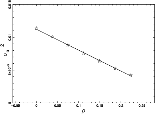
Figure 5: Variance of cells area versus thickness. The stars represent the results of the simulations and the line the theoretical variance, as given by formula (19).

Numerical values of $\sigma^{2}_{a_{0}}$ and $C(h(a_{0})a_{0},a_{0})$ are shown in Table 1.

4 Fitting area distributions of thick Voronoi diagrams

We consider now the probability density function (PDF) of $a$; as noted earlier PDFs of Voronoi cell size are commonly expressed in terms of a standardized variable $x$, which, in the present case, takes the form $x=a/<a>$, so that, obviously, $\langle x\rangle=1$. For future reference, we compute the variance $\sigma^{2}_{x}$ of $x$, which is given by

$$\sigma^{2}_{x}=\frac{\sigma^{2}_{a}}{\langle a\rangle^{2}},$$ (20)

from which, making use of Eqs. (14) and (19),

$$\sigma^{2}_{x}=\frac{\sigma^{2}_{a}}{\langle a\rangle^{2}}\approx\frac{\sigma^{2}_{a_{0}}-2C(h(a_{0})a_{0},a_{0})\rho}{\left<a_{0}-a_{0}h(a_{0})\rho\right>^{2}}.$$ (21)

Values of $\sigma^{2}_{x}$ provided by Eq. (21) are in good agreement with the results of simulations as shown in Fig. 6.

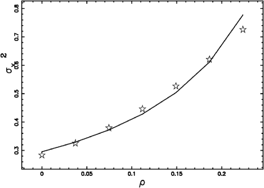
Figure 6: Variance of the standardized variable $x$ versus thickness. The stars represent the results of the simulations and the full line reports the theoretical variance as given by formula (21).

To investigate the distribution of cell areas, we have used the probability density function (4) : however, since $\sigma^{2}_{x}$ increases with $\rho$, from Eq. (6) it is clear that, in order to use the PDF $f$ to fit histograms of simulated data, $d$ must be considered to be a variable parameter which decreases for increasing $\rho$. From Eqs. (6) and (21), it is straightforward to derive a formula for $d$:

$$d(\rho)=\frac{1}{3}\left(\frac{2}{\sigma_{x}^{2}}-1\right)=\frac{1}{3}\left[\frac{2\left<a_{0}-a_{0}h(a_{0})\rho\right>^{2}}{\sigma^{2}_{a_{0}}-2C(h(a_{0})a_{0},a_{0})\rho}-1\right].$$ (22)

Empirical values of $d$ have been found by the method of matching moments and are shown in Fig. 7, together with the fit provided by Eq. (22).

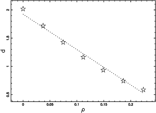
Figure 7: The dimension $d$ that models the Voronoi cell standardized area-distribution in 2D as function of the adimensional parameter $\rho$ (dotted line), see formula (22) and simulated points (stars) .

We have generated histograms of area distribution for different values of $\rho$ and have used the PDF $f$ with the corresponding parameter $d$ derived with Eq. (22): statistical tests show that $\chi^{2}_{\nu}$ increases with $\rho$ and that $\chi^{2}_{\nu}\leq 1.53$ up to $\rho=0.04$ (see Fig. 8), thus the fit is adequate only for very small values of $\rho$.

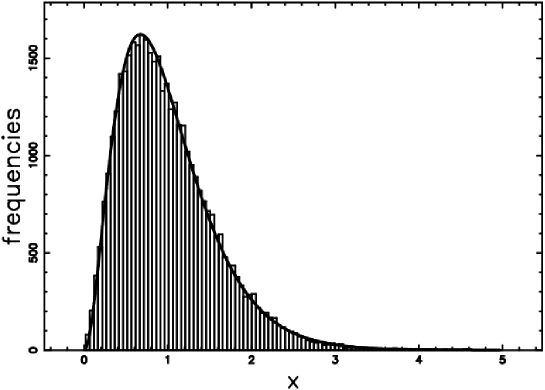
Figure 8: Histogram (step-diagram) of the Voronoi normalized thick area distribution in 2D with a superposition of the gamma PDF derived by Eq. (4), with $d$ given by Eq. (22). The number of seeds and bins are 40000 and 100 respectively: here $d=1.71$ , $\rho=0.04$ , $\chi^{2}=151$ $\chi_{\nu}^{2}=1.53$ .

Even though the PDF $f$, with $d$ given by Eq. (22), gives good results only for small $\rho$ values, it can be used to predict, at least qualitatively, the change in shape of the empirical distribution. The decrease of the parameter $d$ implies a shift of the mode $a_{m}$ toward zero (see Eq.( 7)) and that occurs also in the histograms generated by the simulations.

The result is the appearance of a PDF decreasing monotonically with $a$, as an example see Figure 9, where is clear that lack of agreement with the modified PDF $f$.

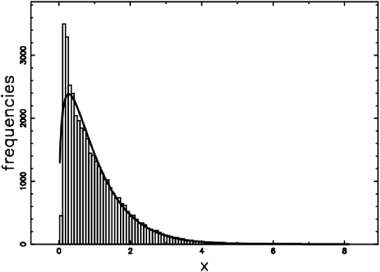
Figure 9: Histogram (step-diagram) of the Voronoi normalized thick area distribution in 2D with a superposition of the gamma PDF as derived by equation (4) with $d$ given by Eq. (22). The number of seeds and bins are 40000 , and 100, respectively, and $\rho=0.22$, $\chi^{2}=5049$ $\chi_{\nu}^{2}=51$ .

5 Conclusions

Voronoi Diagrams in 2D are usually generated as irregular polygons whose edges, in principle, have zero thickness: however in several experimental situations, Voronoi cells appear to have edges of relatively large width.

Clearly the emergence of thick edges is related to the formation of configurations representing approximate Voronoi diagrams, as results of chemical and phy sical mechanisms, are in general quite complex.

Consider, for instance, pattern formation in certain animals coats (e.g. giraffe) by reaction diffusion processes. Here two-dimensional Voronoi diagrams are generated by an activator $a$, diffusing from randomly placed point sources, which switches on the production of melanin, this switch being controlled by a threshold $\theta$ [19]; in a more complex model [20] melanin production is modulated by the concentration of a substrate $s$. Thickness of edges is then determined by the value of $\theta$ [19], or by the abundance and removal rate of the substrate [20].

Voronoi cells can also be generated when an homogeneous medium is occupied by domains emerging from random placed seeds with the same isotropic growth rate [28, 29]: such is the case of crystals [28, 29] or bubbles in volcanic eruptions [30]. In this case the width of the edges can be determined by the relation between the amount of growth and the size of the domain where it takes place.

Edges width should be constant, at least approximately, when processes leading to the formation of Voronoi cells are symmetric, whereas if symmetry breaks down edges of different thickness must be expected. Consider again animal coat formation: if the threshold $\theta$ is not constant over the domain where cells are formed edges of different width will emerge. The same effect can result if the constant value of $\theta$ is replaced by a probability distribution $p(\theta)$.

Here a general method has been presented to compute the statistics of cell areas as the thickness parameter $\rho$ varies: here, for each value of $\rho$, edges have the same width. Theoretical computations as well as results of simulations show that the mean area $\langle a\rangle$ and variance $\sigma^{2}_{a}$ fall off linearly for $\rho$ increasing in the interval $[0,0.2]$: in particular the mean area shows a marked decrease and at $\rho=0.2$ is reduced to $50\%$ of its original value.

We have tried to fit the simulated distribution of the standardized variable $x=a/\langle a\rangle$ with the PDF presented in [21], by using $d$ as a free parameter, but such a fit holds only for $\rho\leq 0.07$; for larger values of $\rho$ simulations show that the mode shifts close to zero more rapidly than predicted by equation Eq. (7).

Finally, it should be noted that the formation of thick edges can be seen as a particular example of a process by which cells are eroded. The approach presented here, however, is general enough to be readily adapted to analyze the statistics of cell areas for different cases of cell erosion, for instance as in diffusion-limited aggregation of Voronoi diagrams [6], in that every erosion operator $k$ must have the form given by Eq. (11) and the terms $h$ and $g$ can be determined from the data, experimental or simulated.

References

- [1] H. G. E. Hentschel, V. Ilyin, N. Makedonska, I. Procaccia, N. Schupper, Phys. Rev. E 75 (5) (2007) 050404–050408.
- [2] J. M. Drouffe, C. Itzykson, Nuc. Phys. B 235 (1984) 45–53.
- [3] L. Zaninetti, Chinese J. Astron. Astrophys. 6 (2006) 387–395.
- [4] G. R. Jerauld, J. C. Hatfield, L. E. Scriven, H. T. Davis, J. Phys. C 17 (1984) 1519–1529.
- [5] S. B. Dicenzo, G. K. Wertheim, Phys. Rev. B 39 (1989) 6792–6796.
- [6] P. A. Mulheran, D. A. Robbie, Europhys. Lett. 49 (2000) 617–623.
- [7] A. Pimpinelli, T. L. Einstein, Phys. Rev. Lett. 99 (22) (2007) 226102–226106.
- [8] J. Ryu, R. Park, D.-S. Kim, Comput. Aided Des. 39 (12) (2007) 1042–1057.
- [9] J. Sudbo, R. Marcelpoil, A. Reith, Anal. Cell. Pathol. 21 (2000) 71–86.
- [10] M. Tanemura, T. Ogawa, N. Ogita, J. Comput. Phys. 51 (1983) 191–207.
- [11] S. Kumar, S. K. Kurtz, J. R. Banavar, M. G. Sharma, J. Stat. Phys 67 (1992) 523–550.
- [12] A. Okabe (Ed.), Spatial tessellations : concepts and applications of voronoi diagrams, Wiley, Chichester, New York, 2000.
- [13] M. Tanemura, Forma 18 (2003) 221–247.
- [14] V. Icke, R. van de Weygaert , A&A 184 (1987) 16–32.
- [15] L. Zaninetti, Phys. Lett. A 373 (2009) 3223–3229.
- [16] F. Giavazzi, R. Cerbino, S. Mazzoni, M. Giglio, A. Vailati, Optic Express 16 (2008) 4819–4823.
- [17] S. Slotterback, M. Toiya, L. Goff, J. F. Douglas, W. Losert, Phys. Rev. Lett. 101 (25) (2008) 258001–258005.
- [18] P. M. Reis, R. A. Ingale, M. D. Shattuck, Phys. Rev. Lett. 96 (25) (2006) 258001–258005.
- [19] J. B. L. Bard, Journal of Theoretical Biology 93 (2) (1981) 363 – 385.
- [20] A. J. Koch, H. Meinhardt, Rev. Mod. Phys. 66 (1994) 1481–1507.
- [21] J.-S. Ferenc, Z. Néda, Phys. A 385 (2007) 518–526.
- [22] A. L. Hinde , R. Miles, J. Stat. Comput. Simul. 10 (1980) 205–223.
- [23] M. Tanemura2005, Statistical distributions of the shape of Poisson Voronoi cells., in: H. Syta (Ed.), Voronoi’s impact on modern science. Book III. Proceedings of the 3rd Voronoi conference on analytic number theory and spatial tessellations, 2005, pp. 193–202.
- [24] T. Kiang, Z. Astrophys. 64 (1966) 433–439.
- [25] W. H. Press, S. A. Teukolsky, W. T. Vetterling, B. P. Flannery, Numerical Recipes in FORTRAN. The Art of Scientific Computing, Cambridge University Press, Cambridge, 1992.
- [26] L. Zaninetti, Journal of Computational Physics 97 (1991) 559–565.
- [27] G. W. Bluman, S. Kumei, Symmetries and Differential Equations, Vol. 81 of Applied Mathematical Sciences, Springer-Verlag, New York-Berlin-Heidelberg-Tokyo, 1989.
- [28] E. Pineda, V. Garrido, D. Crespo, Phys. Rev. E 75 (2007) 040107.
- [29] E. Pineda, D. Crespo, Phys. Rev. E 78 (2008) 021110.
- [30] J. Blower, J. Keating, H. Mader, J. Phillips, Journal of Volcanology and Geothermal Research 120 (1-2) (2002) 1 – 23.