Synchronous motion of two vertically excited planar elastic pendula

M. Kapitaniak^a,b∗, P. Perlikowski^a, T. Kapitaniak^a

$*$corresponding author: m.kapitaniak@abdn.ac.uk

^aDivision of Dynamics, Lodz University of Technology, Stefanowskiego 1/15, 90-924 Lodz, Poland

^bCentre for Applied Dynamics Research, School of Engineering, University of Aberdeen, AB24 3UE, Aberdeen, Scotland, United Kingdom

 

Abstract

The dynamics of two planar elastic pendula mounted on the horizontally excited platform have been studied. We give evidence that the pendula can exhibit synchronous oscillatory and rotation motion and show that stable in-phase and anti-phase synchronous states always co-exist. The complete bifurcational scenario leading from synchronous to asynchronous motion is shown. We argue that our results are robust as they exist in the wide range of the system parameters.

Keywords: coupled oscillators, elastic pendulum, synchronization

 

1 Introduction

The elastic pendulum is a simple mechanical system which comprises heavy mass suspended from a fixed point by a light spring which can stretch but not bend when moving in the gravitational field. The state of the system is given by three (spherical elastic pendulum) or two (planar elastic pendulum) coordinates of the mass, i.e. the system has three (spherical case) or two (planar case) degrees of freedom. The equations of motion are easy to write but, in general, impossible to solve analytically, even in the Hamiltonian case. The elastic pendulum exhibits a wide and surprising range of highly complex dynamic phenomena [1, 2, 3, 4, 5, 6, 7, 8, 9, 10, 11, 12, 13, 14, 15, 16].

For small amplitudes perturbation techniques can be applied, the system is integrable and approximate analytical solutions can be found. The first known study of the elastic pendulum was made by Vitt and Gorelik [17]. They considered small oscillations of the planar pendulum and identified the linear normal modes of two distinct types, vertical or springing oscillations in which the elasticity is the restoring force and quasi-horizontal swinging oscillations in which the system acts like a pendulum. When the frequency of the springing and swinging modes are in the ratio $2:1$, an interesting non-linear phenomenon occurs, in which the energy is transferred periodically back and forth between the springing and swinging motions [1, 2, 3, 4, 5, 6]. The most detailed treatment of small amplitude oscillations of both plane and spherical elastic pendula is presented in the works of Lynch and his collaborators [7, 10, 11, 12]. For large finite amplitudes the system exhibits different dynamical bifurcations and can show chaotic behavior [8, 9, 13, 14, 15, 16].

The dynamics of elastic pendulum attached to linear forced oscillator has been studied by Sado [18]. She has shown a one parameter bifurcation diagrams showing different behaviour of the systems (periodic, quasiperiodic and chaotic). According to our knowledge this is the only study of considered systems, but one can find a lot of papers concerning dynamics of classical pendulum attached to linear or non-linear oscillator. Hatwal et al. [19, 20, 21] gives approximate solutions in the primary parametric instability zone, which allows calculation of the separate regions of periodic solutions. Further analysis enables us to understand the dynamics around primary and secondary resonances [22, 23, 24, 25, 26]. Then the analysis was extended to systems with non-linear base where non-linearity is usually introduced by changing the linear spring into nonlinear one [27, 28, 29, 30] or magnetorheological damper [31]. Recently the complete bifurcation diagram of oscillating and rotating solutions has been presented [32]. Dynamics of two coupled single-well Duffing oscillators forced by the common signal has been investigated in our previous papers [33, 34]. We have shown the detailed analysis of synchronization phenomena and compare different methods of synchronization detection.

In this paper we study the dynamics of two planar elastic pendula mounted on the horizontally excited platform. Our aim is to identify the possible synchronous states of two pendula. We give evidence that the pendula can synchronize both in the oscillatory and rotational motion moreover in-phase and anti-phase synchronizations co-exist. Our calculations have been performed using software Auto–07p [35] developed for numerical continuation of the periodic solutions and verified by the direct integration of the equations of motion. We argue that our results are robust as they exist in the wide range of the system parameters.

The paper is organized as follows. Sec. 2 describes the considered model. We derive the equations of motion and identify the possible synchronization states. In Sec. 3 we study the stability of different types of synchronous motion. Finally Sec. 4 summarizes our results.

2 Model of the system

The analyzed system is shown in Fig. 1. It consists of two identical elastic pendula of length $l_{0}$, spring stiffness $k_{2}$ and masses $m$, which are suspended on the oscillator. The oscillator consists of a bar, suspended on linear spring with stiffness $k_{1}$ and linear viscous damper with damping coefficient $c_{1}$. The system has five degrees of freedom. Mass $M$ is constrained to move only in vertical direction and thus is described by the coordinate $y$. The motion of the first pendulum is described by angular displacement $\varphi$ and its mass by coordinate $x_{2}$, that represent the elongation of the elastic pendulum. Similarly the second pendulum is described by angular displacement $\phi$ and its mass by coordinate $x_{3}$. Both pendula are damped by torques with identical damping coefficient $c_{2}$, that depend on their angular velocities (not shown in Fig. 1). The small damping, with damping coefficient $c_{3}$ is also taken for pendula masses. The system is forced parametrically by vertically applied force $F(t)=F_{0}\cos\nu t$, acting on the bar of mass $M$, that connects the pendula. Force $F_{0}$ denotes the amplitude of excitation and $\nu$ the excitation frequency.

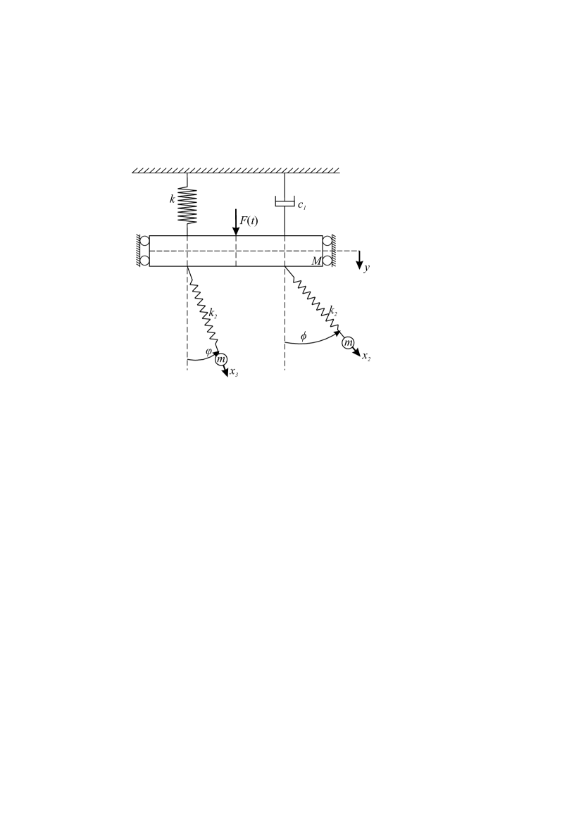
Figure 1: Model of the system

The equations of motion can be derived using Lagrange equations of the second type. The kinetic energy $T$, potential energy $V$ and Rayleigh dissipation $D$ are given respectively by:

$$\hskip 28.45274pt\begin{array}[]{c}T=\frac{1}{2}(M+2m)\dot{y}{}^{2}+\frac{1}{2}m\dot{x}_{3}^{2}+\frac{1}{2}m(l_{0}+y_{wst2}+x_{3})^{2}\dot{\phi}^{2}+m\dot{y}\dot{x}_{3}\cos\phi-m\dot{y}\dot{\phi}(l_{0}+y_{wst2}+x_{3})\sin\phi+\end{array}$$ (2)

$$\hskip 28.45274pt+\frac{1}{2}m\dot{x}_{2}^{2}+\frac{1}{2}m(l_{0}+y_{wst2}+x_{2})^{2}\dot{\varphi}^{2}+m\dot{y}\dot{x}_{2}\cos\varphi-m\dot{y}\dot{\varphi}(l_{0}+y_{wst2}+x_{2})\sin\varphi$$

$$\hskip 28.45274pt\begin{array}[]{c}V=-mg(l_{0}+y_{wst2}+x_{2})\cos\varphi-mg(l_{0}+y_{wst2}+x_{3})\cos\phi+mg(l_{0}+y_{wst2})+mg(l_{0}+y_{wst2})+\end{array}$$ (4)

$$\hskip 28.45274pt+\frac{1}{2}k_{1}(y+y_{wst1})^{2}+\frac{1}{2}k_{2}(y_{wst2}+x_{2})^{2}+\frac{1}{2}k_{2}(y_{wst2}+x_{3})^{2}-(M+2m)gy$$

$$\hskip 28.45274ptD =\frac{1}{2}C_{2}\dot{\varphi}^{2}+\frac{1}{2}C_{2}\dot{\phi}^{2}+\frac{1}{2}C_{3}\dot{x}_{2}^{2}+\frac{1}{2}C_{3}\dot{x}_{3}^{2}$$ (5)

where $c_{3}$ is the damping coefficient of the pendulum mass and $y_{wst1}=\frac{(M+2m)g}{k_{1}}$, $y_{wst2}=\frac{mg}{k_{2}}$ represent static deflation of mass $M$ and pendulums’ mass $m$ respectively. The system is described by five second order differential equations given in the following form:

$$\hskip 28.45274pt\begin{array}[]{c}m(l_{0}+y_{wst2}+x_{2})^{2}\ddot{\varphi}+2m(l_{0}+y_{wst2}+x_{2})\dot{\varphi}\dot{x}_{2}-m\ddot{y}(l_{0}+y_{wst2}+x_{2})\sin\varphi+\end{array}$$ (7)

$$\hskip 28.45274pt+mg(l_{0}+y_{wst2}+x_{2})\sin\varphi+C_{2}\dot{\varphi} =0$$

$$\begin{array}[]{c}\hskip 28.45274ptm(l_{0}+y_{wst2}+x_{3})^{2}\ddot{\phi}+2m(l_{0}+y_{wst2}+x_{3})\dot{\phi}\dot{x}_{3}-m\ddot{y}(l_{0}+y_{wst2}+x_{3})\sin\phi+\end{array}$$ (9)

$$\hskip 28.45274pt+mg(l_{0}+y_{wst2}+x_{3})\sin\phi+C_{2}\dot{\phi} =0$$

$$\hskip 28.45274ptm\ddot{x}_{3}+m\ddot{y}\cos\phi-m\dot{\phi}^{2}(l_{0}+y_{wst2}+x_{3})-mg\cos\phi+k_{2}(y_{wst2}+x_{3})+C_{3}\dot{x}_{3} =0$$ (10)

$$\hskip 28.45274ptm\ddot{x}_{2}+m\ddot{y}\cos\varphi-m\dot{\varphi}^{2}(l_{0}+y_{wst2}+x_{2})-mg\cos\varphi+k_{2}(y_{wst2}+x_{2})+C_{3}\dot{x}_{2} =0$$ (11)

$$\begin{array}[]{c}\hskip 28.45274pt(M+2m)\ddot{y}+m\ddot{x}_{3}\cos\phi-2m\dot{x}_{3}\dot{\phi}\sin\phi-m(l_{0}+y_{wst2}+x_{3})\ddot{\phi}\sin\phi-m(l_{0}+y_{wst2}+x_{3})\dot{\phi}^{2}\cos\phi+\end{array}$$ (13)

$$\hskip 28.45274pt+m\ddot{x}_{2}\cos\varphi-2m\dot{x}_{2}\dot{\varphi}\sin\varphi-m(l_{0}+y_{wst2}+x_{2})\ddot{\varphi}\sin\varphi-m(l_{0}+y_{wst2}+x_{2})\dot{\varphi}^{2}\cos\varphi+$$

$$\hskip 28.45274pt-(M+2m)g+k_{1}(y+y_{wst1})+C_{1}\dot{y}-F_{0}\cos\nu t =0$$

In the numerical calculations we use the following values of parameters: $M=10\hskip 3.61371pt[\textrm{kg]}$, $m=0.2\hskip 3.61371pt[\textrm{kg]}$, $l_{0}=0.24849\hskip 3.61371pt[\textrm{m]}$, $k_{1}=1642.0\hskip 3.61371pt[\textrm{$\frac{N}{m}$]}$, $k_{2}=19.7\hskip 3.61371pt[\textrm{$\frac{N}{m}$]}$, $c_{1}=13.1\hskip 3.61371pt[\textrm{$\frac{Ns}{m}$]}$ , $c_{2}=0.00776\hskip 3.61371pt[\textrm{Nms]}$, $c_{3}=0.49\hskip 3.61371pt[\textrm{$\frac{Ns}{m}$]}$, $y_{wst1}=0.062\hskip 3.61371pt[\mathrm{m}]$, $y_{wst2}=0.1\hskip 3.61371pt[\mathrm{m}]$.

Introducing dimensionless time $\tau=\omega_{1}t$, where $\omega_{1}^{2}=\frac{k_{1}}{M+2m}$ is the natural frequency of mass $M$ with the attached pendula, we obtain dimensionless equations of motion written as:

$$\hskip 19.91684pt\ddot{\Psi}+\frac{2\beta_{2}}{(1+y_{2st}+\chi_{2})}\dot{\Psi}\dot{\chi}_{2}-\frac{\beta_{1}^{2}}{(1+y_{2st}+\chi_{2})}\ddot{\gamma}\sin\Psi+\frac{\sin\Psi}{(1+y_{2st}+\chi_{2})}+\frac{\alpha_{2}}{(1+y_{2st}+\chi_{2})^{2}}\dot{\Psi} =0$$ (14)

$$\hskip 19.91684pt\ddot{\Phi}+\frac{2\beta_{2}}{(1+y_{2st}+\chi_{3})}\dot{\Phi}\dot{\chi}_{3}-\frac{\beta_{1}^{2}}{(1+y_{2st}+\chi_{3})}\ddot{\gamma}\sin\Phi+\frac{\sin\Phi}{(1+y_{2st}+\chi_{3})}+\frac{\alpha_{2}}{(1+y_{2st}+\chi_{3})^{2}}\dot{\Phi} =0$$ (15)

$$\hskip 19.91684pt\ddot{\chi}_{3}+\frac{\beta_{1}^{2}}{\beta_{2}^{2}}\ddot{\gamma}\cos\Phi-\frac{1+y_{2st}+\chi_{3}}{\beta_{2}^{2}}\dot{\Phi}^{2}-\frac{1}{\beta_{2}^{2}}\cos\Phi+y_{st2}+\chi_{3}+\alpha_{3}\dot{\chi}_{3} =0$$ (16)

$$\hskip 19.91684pt\ddot{\chi}_{2}+\frac{\beta_{1}^{2}}{\beta_{2}^{2}}\ddot{\gamma}\cos\Psi-\frac{1+y_{2st}+\chi_{2}}{\beta_{2}^{2}}\dot{\Psi}^{2}-\frac{1}{\beta_{2}^{2}}\cos\Psi+y_{st2}+\chi_{2}+\alpha_{3}\dot{\chi}_{2} =0$$ (17)

$$\hskip 19.91684pt\begin{array}[]{c}\ddot{\gamma}+\frac{\beta_{2}^{2}a}{\beta_{1}^{2}}\ddot{\chi}_{3}\cos\Phi-\frac{2\beta_{2}a}{\beta_{1}^{2}}\dot{\chi}_{3}\dot{\Phi}\sin\Phi-\frac{(1+y_{2st}+\chi_{3})a}{\beta_{1}^{2}}\ddot{\Phi}\sin\Phi-\frac{(1+y_{2st}+\chi_{3})a}{\beta_{1}^{2}}\dot{\Phi}^{2}\cos\Phi+\frac{\beta_{2}^{2}a}{\beta_{1}^{2}}\ddot{\chi}_{2}\cos\Psi+\end{array}$$ (19)

$$\hskip 19.91684pt-\frac{2\beta_{2}a}{\beta_{1}^{2}}\dot{\chi}_{2}\dot{\Psi}\sin\Psi-\frac{(1+y_{2st}+\chi_{2})a}{\beta_{1}^{2}}\ddot{\Psi}\sin\Psi-\frac{(1+y_{2st}+\chi_{2})a}{\beta_{1}^{2}}\dot{\Psi}^{2}\cos\Psi-\frac{1}{\beta_{1}^{2}}+\gamma+y_{1st}+\alpha_{1}\dot{\gamma}-q\cos\mu\tau =0$$

where $\omega_{2}^{2}=\frac{k_{2}}{m}$, $\omega_{4}^{2}=\frac{g}{l_{0}}$, $\mu=\frac{\nu}{\omega_{1}}$, $\beta_{1}=\frac{\omega_{1}}{\omega_{4}}$, $\beta_{2}=\frac{\omega_{2}}{\omega_{4}}$, $a=\frac{m}{M+2m}$, $q=\frac{F_{0}}{\omega_{1}^{2}l_{0}(M+2m)}$, $\alpha_{1}=\frac{C_{1}}{\omega_{1}(M+2m)}$, $\alpha_{2}=\frac{C_{2}}{m\omega_{4}l_{0}^{2}}$, $\alpha_{3}=\frac{C_{3}}{ml_{0}\omega_{2}^{2}}$, $y_{1st}=\frac{y_{wst1}}{l_{0}}$, $y_{2st}=\frac{y_{wst2}}{l_{0}}$, $\gamma=\frac{y}{l_{0}}$, $\dot{\gamma}=\frac{\dot{y}}{l_{0}\omega_{4}}$, $\ddot{\gamma}=\frac{\ddot{y}}{l_{0}\omega_{4}^{2}}$, $\chi_{3}=\frac{x_{3}}{l_{0}}$, $\dot{\chi}_{3}=\frac{\dot{x}_{3}}{l_{0}\omega_{2}}$, $\ddot{\chi}_{3}=\frac{\ddot{x}_{3}}{l_{0}\omega_{2}^{2}}$,$\chi_{2}=\frac{x_{2}}{l_{0}}$, $\dot{\chi}_{2}=\frac{\dot{x}_{2}}{l_{0}\omega_{2}}$, $\ddot{\chi}_{2}=\frac{\ddot{x}_{2}}{l_{0}\omega_{2}^{2}}$, $\Psi=\varphi$, $\dot{\Psi}=\frac{\dot{\varphi}}{\omega_{4}}$, $\ddot{\Psi}=\frac{\ddot{\varphi}}{\omega_{4}^{2}}$, $\Phi=\phi$, $\dot{\Phi}=\frac{\dot{\phi}}{\omega_{4}}$, $\ddot{\Phi}=\frac{\ddot{\phi}}{\omega_{4}^{2}}$

The dimensionless parameters of the system have the following values: $\beta_{1}=2$, $\beta_{2}=1.58$, $\alpha_{1}=0.1$, $\alpha_{2}=0.01$, $\alpha_{3}=0.1$, $a=0.0192$, $y_{1st}=0.25$, $y_{2st}=0.4$.

We study system (9-13) in order to detect possible synchronization ranges. There are two basic types of synchronous motion, which are depicted in Fig. 2(a,b). The pendula can synchronize either in-phase or in anti-phase with each other, i.e., $\Psi=\Theta$ or $\Psi=-\Theta$. In both mentioned cases the forces acting in vertical direction on mass $M$ are identical (there are no forces in horizontal direction), hence the energy transmitted between mass $M$ and pendula in in-phase and anti-phase motion is also identical. If there is an in-phase synchronization, the anti-phase also coexists in the same range of parameters. The accessibility of in-phase and anti-phase motion is governed only by initial conditions. The pendula’s masses are always synchronized in the in-phase with each other, i.e., $\chi_{2}=\chi_{3}$. The anti-phase configuration of the masses is not observed $(\chi_{2}=-\chi_{3})$ with the oscillating pendula. The anti-phase synchronization of masses is possible when the pendula are in equilibrium positions, then the sum of forces transmitted to mass $M$ is equal to zero.

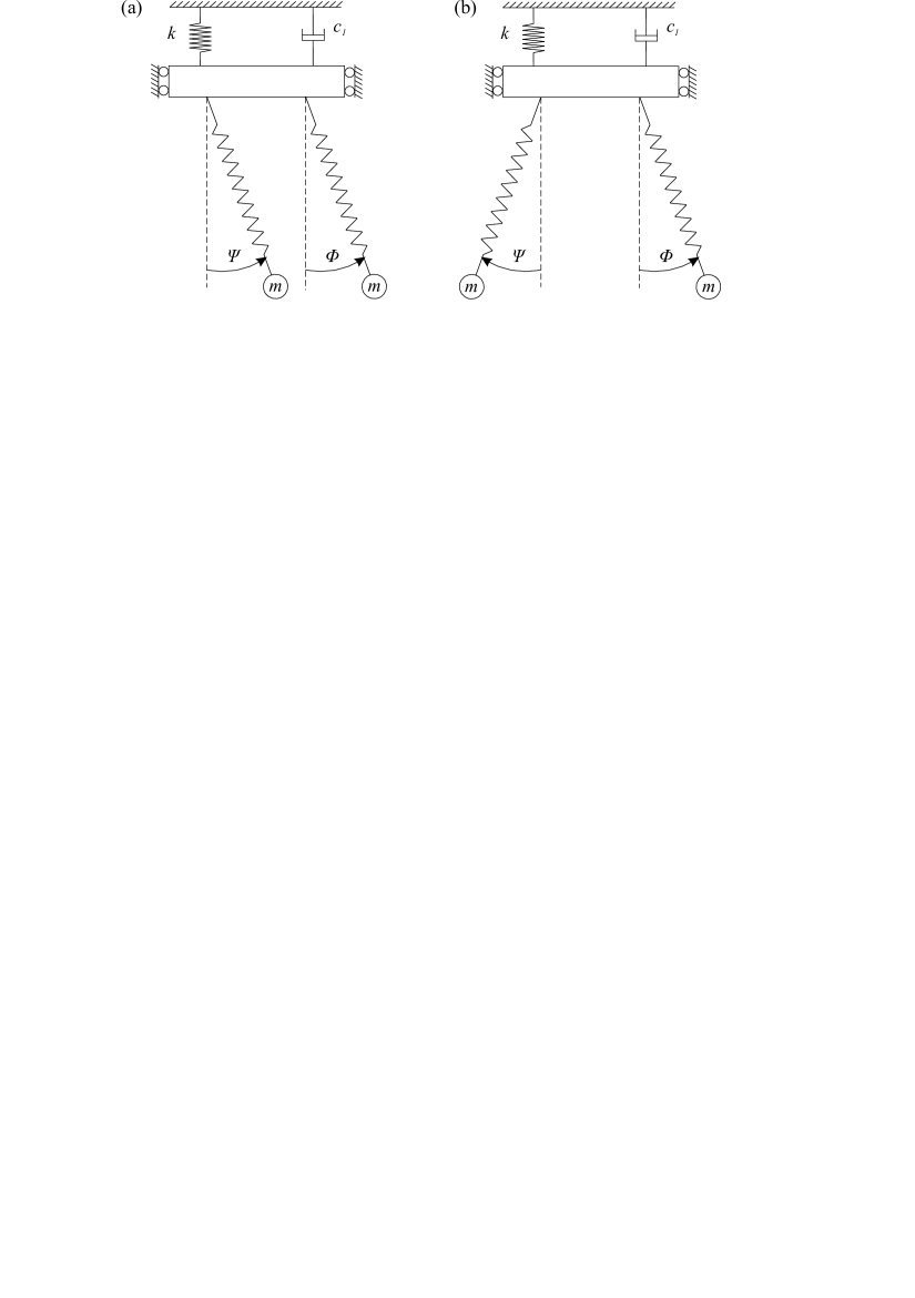
Figure 2: Possible synchronization (a) in-phase, (b) in anti-phase

3 Stability of synchronous motion

3.1 Synchronous solutions in two dimensional parameters space

In this section we study the stability of the observed synchronous oscillations and rotations of the pendula. We present the bifurcation diagrams calculated in two-parameter space: amplitude $q$ versus frequency $\mu$ of excitation. We focus our attention on determining the regions of synchronous stable motion and bifurcations that lead to its destabilization. We consider the state of the system in the following range $q\in[0.0,\>1.2]$ of forcing amplitudes and frequency of excitation belonging to the range $\mu\in[0.3,\>1.2]$, which cover the possible resonances in the system. Resonance should be observed when the frequency of excitation comes close to the natural frequencies: of mass $M$ equal to $\mu_{M}=1$, of pendula $\mu_{p}=0.50$ and pendulum mass $\mu_{pm}=0.79$. We describe synchronous solutions with respect to the forcing period according to ratio $r:1-s:1$, where $r$ and $s$ denotes number of forcing periods, for which pendula and pendula masses perform period one motion. Fig. 3 presents two parameter bifurcation diagram, obtained by direct integration of (9-13). It shows the existence of synchronous, asynchronous motion and equilibrium solutions. As soon as we have a lot of coexisting solutions to hold clearance of Fig. 3 we do not distinguish which type of synchronous or asynchronous we find. By synchronous solution we mean, that both pendula are in complete synchronization state, i.e., their amplitudes and frequencies are identical. For low amplitudes of excitation, the only solution is equilibrium, which turns into synchronous or asynchronous solution as the frequency of excitation increases. The detailed analysis of synchronous solutions (shaded in grey color) was performed using continuation software Auto–07p [35]. We calculate the stability borders of each identified case, i.e., the ranges inside which the given motion is stable. The first periodic solution is observed for frequency of excitation equal to $\mu=0.406$ and for amplitudes of excitation above $q=0.709$. This periodic solution is shown in Fig. 4(a) is identified as synchronous oscillations of pendula and pendula masses locked $1:1-1:1$ with forcing. This solution is destabilized by saddle-node (green line), period doubling (blue line) and Neimark-Sacker (red line) bifurcations curves. The continuation reveals that for small range of parameters, around the frequency of excitation close to the natural frequency of pendula, this solution coexists with synchronous $2:1-1:1$ oscillations. Synchronous oscillations $2:1-1:1$ are destabilized by saddle-node bifurcation curve then by Neimark-Sacker and pitchfork symmetry breaking (SB2) bifurcations. In the investigated system we distinguish two different symmetry breaking pitchfork bifurcations one of them (SB2) brokes symmetry between the pendula, the second one (SB1) brokes the symmetry of each pendula but their motion remains identical [36]. As the frequency of excitation increases we observe either asynchronous motion or equilibrium. With further increase of excitation frequency we observe asynchronous behavior, which change into two small regions of synchronous rotations $3:1-1:1$. We show it in Fig. 4(f) and this area is bounded by Neimark-Sacker, period doubling and saddle-node bifurcations. This solution coexists with synchronous $2:1-1:1$ rotations, presented also in Fig. 4(f). The stability region for this solution is bounded by pitchfork SB1 bifurcation from the left and right, Neimark-Sacker from above, and saddle-node and Neimark-Sacker bifurcations from the right. Both these solutions coexist in small range of considered parameters with another synchronous rotations $4:1-1:1$, presented in Fig. 4(f). The synchronous motion destabilizes from the right by saddle-node and pitchfork SB2 curves, from above by Neimark-Sacker, and from the left by Neimark-Sacker, saddle-node and pitchfork SB2 curves.

Around $\mu\approx 0.8$, where the resonance of pendulum masses occur, the system possesses rich dynamics, which results in the coexistence of different synchronous together with asynchronous solutions. This includes synchronous rotations $2:1-1:1$ depicted in Fig. 4(c,d) and synchronous $3:1-3:1$ rotations of pendula and pendula masses presented in Fig. 4(e). The third which was found solution is synchronous half-rotations $1:1-1:1$ (Fig. 4(b)), for which both pendula stop before approaching stable and unstable equilibrium transferring the whole energy into displacement of pendula masses. This multistability causes that it is hard to compare the bifurcation diagrams from the direct integration and Auto-07p. In the case of rotations $2:1-1:1$ the synchronous motion is destabilzed from the right by saddle-node and pitchfork SB2 curves, from above by Neimark-Sacker, and from the left by saddle-node, Neimark-Sacker and pitchfork SB2 bifurcations. Synchronous rotations $1:1-1:1$ loose stability by pitchfork SB2 from the right, and by Neimark-Sacker and period doubling from the left. The synchronous rotations $3:1-3:1$ are mainly destabilized by pitchfork SB2 from the right and by pitchfork SB2 and period doubling from the bottom, and by period doubling, pitchfork SB2, saddle-node and Neimark-Sacker from the left. From this solution, through period-doubling bifurcation we find synchronized rotations $6:1-6:1$, shown in Fig. 4(e). This solution is destabilized from above by period-doubling bifurcation, from the left through pitchfork SB2 bifurcation, and from below through saddle-node bifurcation (not visible, since coincides with period-doubling boundary for rotations $3:1-3:1$).

As we pass through the resonance frequency of mass $M$ equal to $\mu=1$, for higher amplitudes of excitation the only synchronous solution includes $2:1-1:1$ synchronous rotations depicted in Fig. 4(c,d). After the resonance, for amplitudes of excitation above $q=0.141$, only asynchronous solutions are observed. Below this value, many small synchronous regions were found. This includes synchronous $1:1-1:1$ oscillations and two regions of synchronous $2:1-1:1$ oscillations, together with two regions of synchronous $2:1-1:1$ rotations. The region of $1:1-1:1$ oscillations is enclosed by saddle-node, Neimark-Sacker and pitchfork SB2 bifurcation curves. Oscillatory $2:1-1:1$ motion destabilizes through pitchfork SB1 from above and Neimark-Sacker curves from below. This solution coexists for small range of parameters with $2:1-1:1$ rotations, which motion is destabilized by period doubling and Neimark-Sacker from the left, and from the right by pitchfork SB2, Neimark-Sacker and period doubling curves. We observe the excellent correlation in these regions between the results from numerical continuation and direct integration.

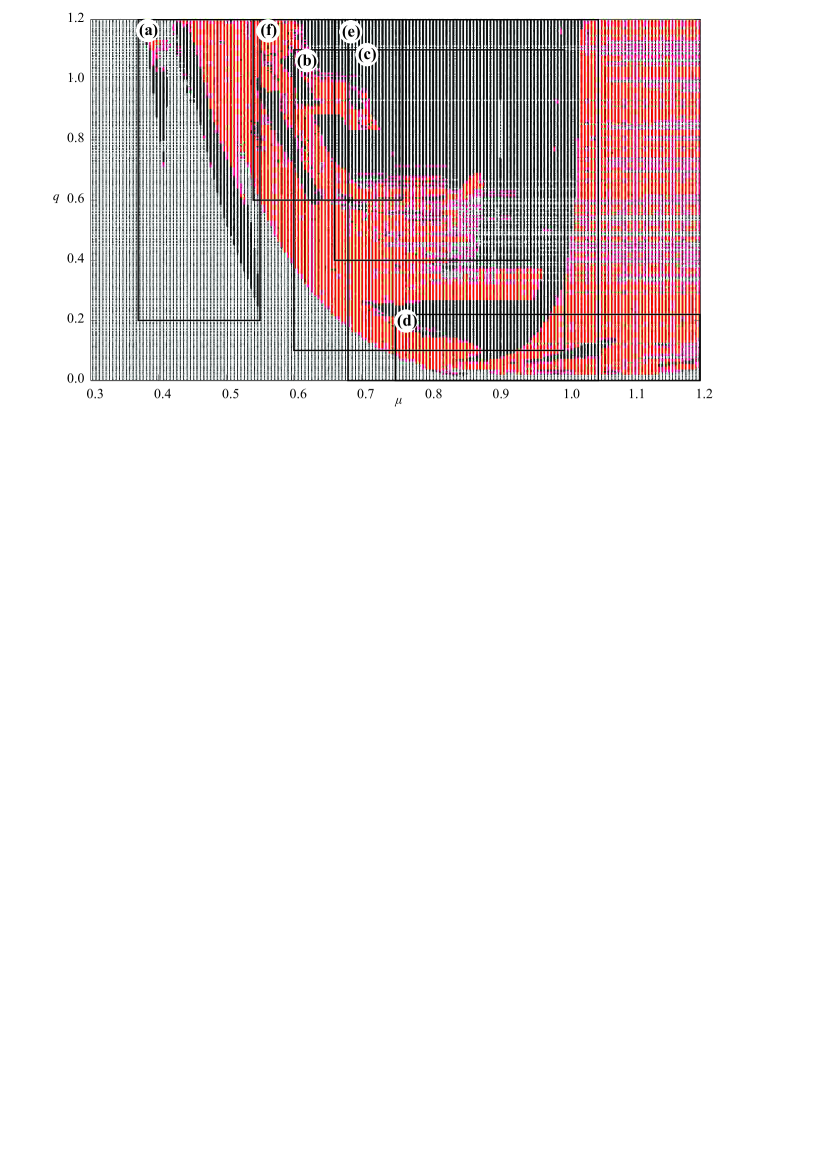
Figure 3: (color online) The synchronous (black dots), asynchronous (red dots) and equilibrium (small grey crosses) solutions of system (9-13) in two parameters space: $\mu$ frequency and $q$ amplitude of excitation. We calculate this plot by direct integration using 4th order Runge-Kutta algorithm. In rectangles (a-f) we highlighted regions of synchronous motion calculated in Auto-07p (see Fig. 4).

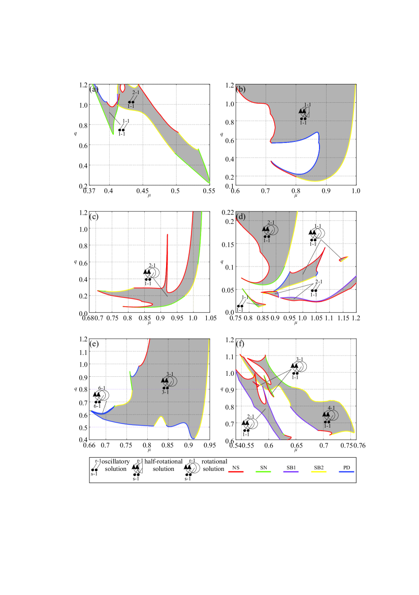
Figure 4: (color) Stable ranges of synchronous motion calculated in Auto-07p (see rectangles in Fig. 3). Color of lines stand for different types of bifurcation: Neimark-Sacker (red), saddle-node (green), pitchfork SB1 (violet), pitchfork SB2 (yellow) and period doubling (blue). In region inside lines synchronous solutions are periodic and stable.

3.2 One parameter continuation

In this subsection we show one parameter continuation of four periodic solutions (two oscillating and two rotational) for fixed amplitude of excitation, as a bifurcation parameter we choose the frequency of excitation $\mu$. We start each path-following on the periodic solution and continue in two directions (forward and backward). In Fig. 5(a-d) we present the synchronized oscillating periodic solutions, their regions of stability are shown in Fig. 4 (a). System (14-19) is given by five second order ODEs, hence the phase space is ten dimensional and at least five figures (amplitude of each degree of freedom) are necessary to show its complete dynamics. To decrease it we focus on the dynamics of first pendula (second pendula has the same amplitude in the synchronized state) and mass $M$. The first presented branch of periodic solutions in Fig. 5(a,b) is synchronous $2:1-1:1$ oscillations, in previous subsection we show that this family is destabilized by Neimark-Sacker bifurcation from the right and from the left by pitchfork symmetry braking SB2. Switching the branch at pitchfork bifurcation enables us to find another stable branch of asynchronized oscillations $2:1-1:1$, that looses its stability through the saddle-node bifurcation. After pitchfork symmetry breaking SB2 bifurcation the solutions of one pendulum is located at upper branch (see Fig. 5(b)) and the second pendulum on lower branch or vice-versa. The branch synchronous oscillations $2:1-1:1$, shown in Fig. 5 (c,d), present much richer scenario than other. These oscillations destabilize from both sides through pitchfork SB2 bifurcation. When we switch branch in left SB2 point, we find family of stable asynchronized oscillations $2:1-1:1$. Finally, when the amplitudes of pendula reach zero their motion stops. When we continue in the opposite direction the stability is lost in pitchfork SB2 bifurcation. Another change of branch allows us to observe another asynchronous periodic solutions, for which first pendulum oscillates $2:1-1:1$, second pendulum is at rest (not shown here) and pendula masses oscillate $1:1-1:1$ in asynchronized manner. One end of this stable branch destabilizes through saddle-node bifurcation and the second one by pitchfork SB2 bifurcation. As the frequency of excitation increases the stability of this solutions is regained through pitchfork SB2 bifurcation and lost again through saddle-node bifurcation. Note that for the mass $M$, the bifurcation points that are responsible for the destabilization of periodic solutions for synchronized oscillations $2:1-1:1$ and asynchronized oscillations $2:1-1:1$, are placed very close to each other. When we switch the branch in the right SB2 bifurcation point of the synchronized oscillations $2:1-1:1$, we find asynchronized solution of oscillations $2:1-1:1$ that persists for small interval of excitation frequency. It destabilizes from above and below through period-doubling bifurcations. Switching the branch in lower period doubling bifurcation point enables us to observe asynchronized oscillations $4:1-2:1$, that destabilize through Neimark-Sacker bifurcation. The bifurcation diagram, shown in Fig. 6(a-b), shows $3:1-3:1$ rotational periodic solutions for $q=0.654$. In contrary to the previous cases, to hold a physical meaning, on the horizontal axis we plot the amplitude of velocity. The stability region of this branch is shown in Fig. 4(e). This family of solutions looses its stability through period-doubling and pitchfork SB2 bifurcations. Switching the branch in the period-doubling bifurcation point, allows to observe another period doubling, which leads us to two branches of synchronized $6:1-6:1$ rotational solution. This branch looses its stability once again through period-doubling bifurcation. After another switch of branch in period doubling bifurcation point, we reach two synchronized periodic $12:1-12:1$ rotational solutions. They are stable in very narrow range of excitation frequency and loosing stability via Neimark-Sacker bifurcations. After switching the branch in right pitchfork SB2 bifurcation point, we observe asynchronized rotations $3:1-3:1$, that are stable in very small interval, finally loosing its stability through saddle-node bifurcation. In Fig. 6(c-d) we present synchronized rotations $4:1-1:1$, that loose stability through pitchfork symmetry braking from the right and left. Switching the branch in both SB2 bifurcation points let us to find asynchronous rotations $4:1-4:1$, that are stable in very narrow interval of excitation frequency, loosing finally stability through saddle-node bifurcation.

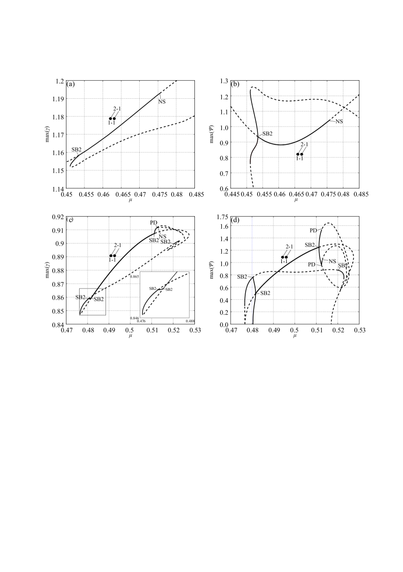
Figure 5: 1 parameter continuation of fully synchronized: 2:1-1:1 oscillations ((a) mass $M$, (b) pendulum 1, $q=0.899$, $\mu=0.455$), 2:1-1:1 oscillations ((c) mass $M$, (d) pendulum 1, $q=0.654$, $\mu=0.5$). The continuous and dashed lines correspond to stable and unstable periodic solutions respectively. Abbreviations depicted following bifurcations: NS (Neimark-Sacker), PD (period doubling), SB1 (pitchfork SB1) and SB2 (pitchfork SB2). Other changes of the stability take place through the saddle-node bifurcations.

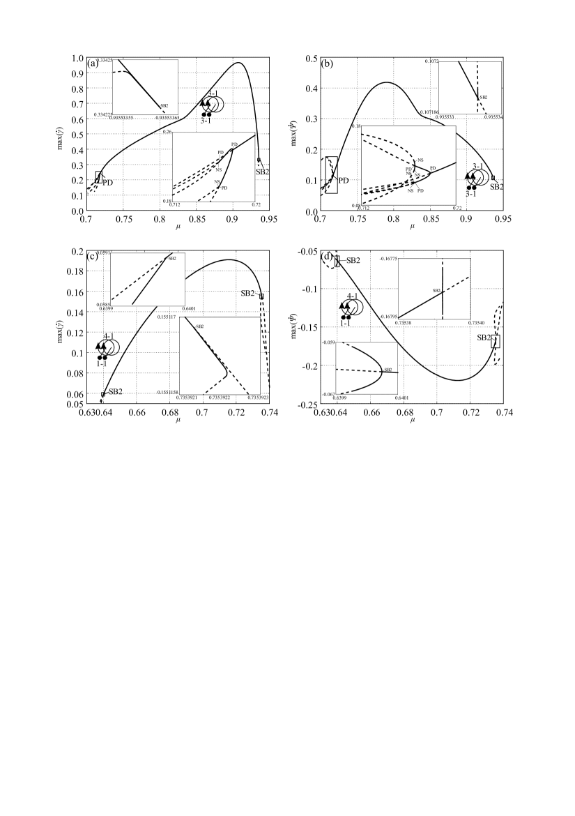
Figure 6: 1 parameter continuation of fully synchronized: $3:1-3:1$ rotations ((a) mass $M$, (b) pendulum 1, $q=0.654$, $\mu=0.8$), $4:1-1:1$ rotations ((c) mass $M$, (e) pendulum 1, $q=0.8$, $\mu=0.7$). The continuous and dashed lines correspond to stable and unstable periodic solutions respectively. Abbreviations depicted following bifurcations: NS (Neimark-Sacker), PD (period doubling), SB1 (pitchfork SB1) and SB2 (pitchfork SB2). Other changes of the stability take place through the saddle-node bifurcations.

4 Conclusions

In the system of two planar elastic pendula suspended on the excited linear oscillator one can observe both in-phase and anti-phase synchronization of the elastic pendula. In-phase and anti-phase synchronous states always co-exist. Pendula can synchronize during the oscillatory and rotational motion but only when their behaviour is periodic. We have not observed the synchronization of the chaotically behaving pendula. This result is contrary to the great number of chaos synchronization examples [37, 38, 39] but confirms the results obtained in [40] where it has been shown that the forced Duffing’s oscillators mounted to the elastic beam can synchronize only after motion become periodic. The synchronization of the chaotic motion of the pendula is impossible as the excited oscillator transfers the same signal to both pendula which cannot differently modify the pendula’s motion. We also have not observed in-phase or anti-phase synchronization of the pendula when masses $m_{2}$ and $m_{3}$ are in anti-phase. With one parameter bifurcation diagrams we present a bifurcational scenario of synchronous solutions. We show a route from synchronous via asynchronous periodic solutions to quasiperiodic and chaotic behaviour. In this case the pendula in-phase or anti-phase synchronization is impossible as the pendula have different and non-constant lengths. In this case one can expect some kind of generalized synchronization but this problem will be addressed elsewhere [41].

We show two dimensional bifurcation diagrams with the most representative periodic solutions in the considered system. In the neighbourhood of the linear resonances of subsystems we have rich dynamics with both periodic and chaotic attractors[42]. Our results are robust as they exit in the wide range of system parameters, especially two dimensional bifurcation diagram can be used as a scheme of bifurcations in the class of systems similar to investigated in this paper.

References

- [1] B. Anicin, D. Davidovic, V. Babovic, On the linear theory of the elastic pendulum, European Journal of Physics 14 (1993) 132–135.
- [2] E. Breitenberger, R. Mueller, The elastic pendulum: A nonlinear paradigm, Journal of Mathematical Physics 22 (6).
- [3] R. Carretero-Gonzalez, H. Nunez-Yepez, A. L. Salas-Brito, Regular and chaotic behaviour in an extensible pendulum, European Journal of Physics 15 (1994) 139–148.
- [4] T. E. Cayton, The laboratory spring-mass oscillator: an example of parametric instability, American Journal of Physics 45 (8).
- [5] R. Cuerno, A. F. Ranada, J. J. Ruiz-Lorenzo, Deterministic chaos in the elastic pendulum: A simple laboratory for nonlinear dynamics, American Journal of Physics 60(1).
- [6] D. Davidovic, B. Anicin, V. Babovic, The libration limits of the elastic pendulum, American Journal of Physics 64(3).
- [7] D. Holm, P. Lynch, Stepwise precession of the resonant swinging spring, SIAM Journal on Applied Dynamical Systems 1 (1) (2002) 44–64.
- [8] S. Kuznetsov, The motion of the elastic pendulum, Regular and Chaotic Dynamics 4 (3).
- [9] H. Lai, On the recurrence phenomenon of a resonant spring pendulum, American Journal of Physics 53(3).
- [10] P. Lynch, Resonant motions of the three dimensional elastic pendulum, International Journal of Non-Linear Mechanics 37 (2002) 345–367.
- [11] P. Lynch, In Norbury J., Roulstone I.(Eds.): Large-scale Atmosphere-Ocean Dynamics, Vol.II, Geometric Methods and Models, Cambridge University Press, Cambridge, 2002, Ch. The swinging spring: a simple model of atmospheric balance, pp. 64–108.
- [12] P. Lynch, C. Houghton, Pulsation and precession of the resonant swinging spring, Physica D 190 (2004) 38–62.
- [13] H. Nunez-Yepez, A. L. Salas-Brito, C. Vargas, L. Vicente, Onset of chaos in an extensible pendulum, Physics Letters A 145 (2,3).
- [14] M. Olsson, Why does a mass on a spring sometimes misbehave?, American Journal of Physics 44 (12).
- [15] P. Pokorny, Stability condition for vertical oscillation of 3-dim heavy spring elastic pendulum, Regular and Chaotic Dynamics 13 (2008) 155–165.
- [16] M. Rusbridge, Motion of the spring pendulum, American Journal of Physics 48 (2).
- [17] A. Vitt, G. Gorelik, Oscillations of an elastic pendulum as an example of the oscillations of two parametrically coupled linear systems, Journal of Technical Physics 3(2-3) (1933) 294–307, translated from Russian by Lisa Shields with an introduction.
- [18] D. Sado, The dynamic of a coupled three degree of freedom mechanical system, Mechanics and Mechanical Engineering 7 (2004) 20–39.
- [19] H. Hatwal, H. Mallik, A. Ghosh, Non-linear vibrations of a harmonically excited autoparametric system, Journal of Sound and Vibration 81 (2) (1982) 153–164.
- [20] H. Hatwal, A. K. Mallik, A. Ghosh, Forced nonlinear oscillations of an autoparametric system—part 1: Periodic responses, Journal of Applied Mechanics 50 (3) (1983) 657–662.
- [21] H. Hatwal, A. K. Mallik, A. Ghosh, Forced nonlinear oscillations of an autoparametric system—part 2: Chaotic responses, Journal of Applied Mechanics 50 (3) (1983) 663–668.
- [22] A. K. Bajaj, S. I. Chang, J. M. Johnson, Amplitude modulated dynamics of a resonantly excited autoparametric two degree-of-freedom system, Nonlinear Dynamics 5 (1994) 433–457.
- [23] M. Cartmell, J. Lawson, Performance enhancement of an autoparametric vibration absorber by means of computer control, Journal of Sound and Vibration 177 (2) (1994) 173 – 195.
- [24] J. Balthazar, B. Cheshankov, D. Ruschev, L. Barbanti, H. Weber, Remarks on the passage through resonance of a vibrating system with two degrees of freedom, excited by a non-ideal energy source, Journal of Sound and Vibration 239 (5) (2001) 1075 – 1085.
- [25] J. Warminski, K. Kecik, Autoparametric vibration of a nonlinear system with pendulum, Mathematical Problems in Engineering 2006 (2006) 80705.
- [26] Y. Song, H. Sato, Y. Iwata, T. Komatzuzaki, The response of a dynamic vibration absorber system with a parametrically excited pendulum, Journal of Sound and Vibration 259 (4) (2003) 747 – 759.
- [27] J. Warminski, K. Kecik, Instabilities in the main parametric resonance area of a mechanical system with a pendulum, Journal of Sound and Vibration 322 (3) (2009) 612 – 628.
- [28] J. Warminski, J. Balthazar, R. Brasil, Vibrations of a non-ideal parametrically and self-excited model, Journal of Sound and Vibration 245 (2) (2001) 363 – 374.
- [29] L. Macias-Cundapi, G. Silva-Navarro, B. Vazquez-Gonzalez, Application of an active pendulum-type vibration absorber for duffing systems, in: Electrical Engineering, Computing Science and Automatic Control, 2008. CCE 2008. 5th International Conference on, 2008, pp. 392 –397.
- [30] B. Vazquez-Gonzalez, G. Silva-Navarro, Evaluation of the autoparametric pendulum vibration absorber for a duffing system, Shock and Vibration 15 (2008) 355–368.
- [31] K. Kecik, J. Warminski, Dynamics of an autoparametric pendulum-like system with a nonlinear semiactive suspension, Mathematical Problems in Engineering.
- [32] P. Brzeski, P. Perlikowski, S. Yanchuk, T. Kapitaniak, The dynamics of the pendulum suspended on the forced duffing oscillator, Submitted to Journal of Sound and Vibration.
- [33] P. Perlikowski, A. Stefanski, T. Kapitaniak, 1:1 mode locking and generalized synchronization in mechanical oscillators, Journal of Sound and Vibration 318 (1-2) (2008) 329 – 340.
- [34] P. Perlikowski, Synchronization of mechanical oscillators excited kinematically, Journal of Theoretical and Applied Mechanics 48 (2008) 185–204.
- [35] E. Doedel, B. Oldeman, A. Champneys, F. Dercole, T. Fairgrieve, Y. Kuznetsov, R. Paffenroth, B. Sandstede, X. Wang, C. Zhang., AUTO-07P: Continuation and Bifurcation Software For Ordinary Differential Equations, Concordia University, Montreal, Canada, 2011.
- [36] J. Miles, Resonance and symmetry breaking for the pendulum, Phys. D 31 (1988) 252–268.
- [37] A. Stefanski, T. Kapitaniak, Estimation of the dominant lyapunov exponent of non-smooth systems on the basis of maps synchronization, Chaos Solitons & Fractals 15 (2003) 233–244.
- [38] A. Stefanski, T. Kapitaniak, Using chaos synchronization to estimate the largest lyapunov exponent of nonsmooth systems, Discrete Dynamics in Nature and society 4 (2000) 207–215.
- [39] Y. Maistrenko, T. Kapitaniak, P. Szuminski, Locally and globally riddled basins in two coupled piecewise-linear maps, Physical Review E 56 (1997) 6393–6399.
- [40] K. Czolczynski, T. Kapitaniak, P. Perlikowski, A. Stefanski, Periodization of duffing oscillators suspended on elastic structure: Mechanical explanation, Chaos Solitons & Fractals 32 (2007) 920–926.
- [41] M. Kapitaniak, P. Perlikowski(in preparation).
- [42] A. Chudzik, P. Perlikowski, A. Stefanski, T. Kapitaniak, Multistability and rare attractors in van der pol-duffing oscillator., I. J. Bifurcation and Chaos 21 (7) (2011) 1907–1912.
- [43] J. Miles, Resonance and symmetry breaking for as duffing oscillator, SIAM J. Appl. Math. 49 (1989) 968–981.