Full bispectra from primordial scalar and tensor perturbations in the most general single-field inflation model

Abstract

We compute the full bispectra, namely both auto- and cross- bispectra, of primordial curvature and tensor perturbations in the most general single-field inflation model whose scalar and gravitational equations of motion are of second order. The formulae in the limits of k-inflation and potential-driven inflation are also given. These expressions are useful for estimating the full bispectra of temperature and polarization anisotropies of the cosmic microwave background radiation.

I Introduction

The non-Gaussianities of the temperature and polarization anisotropies of the cosmic microwave background (CMB) radiation now receive increasing attentions because they are important tools to discriminate models of inflation oriinf ; r2 . Ongoing and near future project such as Planck satellite Planck:2006aa , CMBpol mission Baumann:2008aq , LiteBIRD satellite LiteBIRD would reveal the properties of the temperature and polarization anisotropies in detail. Such E-mode polarization anisotropies are sourced by both curvature and tensor perturbations polar , while only tensor (and vector) perturbations can generate B-mode polarization anisotropies Zaldarriaga:1996xe . Therefore, even when one estimates the “auto” bispectra of the temperature and the E-mode polarization fluctuations, not only the auto bispectra but also the cross bispectra of the primordial curvature and tensor perturbations are indispensable.

For slow-roll inflation models with the canonical kinetic term slowroll , Maldacena evaluated the full bispectra, including the cross bispectra, of the primordial curvature and tensor perturbations Maldacena:2002vr . Inflation models are now widely generalized into more varieties such as k-inflation ArmendarizPicon:1999rj , DBI inflation Silverstein:2003hf , ghost inflationArkaniHamed:2003uz , G-inflation Kobayashi:2010cm , and so on. However, almost all the works on the non-Gaussianities in these inflation models concentrate only on the auto bispectrum of the curvature perturbations Seery:2005wm ; Alishahiha:2004eh ; Mizuno:2010ag , which is insufficient for evaluating the bispectra of the temperature and E-mode polarization anisotropies of the CMB, as explained above. To our surprise, as far as we know, the full bispectra of the primordial curvature and tensor perturbations have not yet been obtained even for k-inflation ArmendarizPicon:1999rj except for Ref. Shiraishi:2010kd where the primordial scalar-scalar-tensor cross bispectrum has been calculated for inflation models with an arbitrary kinetic term. There are several related works on the primordial cross bispectra. In Ref. McFadden:2011kk , the authors show the primordial tensor-scalar cross bispectra induced from a holographic model and the scalar-scalar-tensor correlation has been discussed in the calculation of the trispectrum of the scalar fluctuations Seery:2008ax , so-called “graviton exchange”, and also in the context of one-loop effects of the scalar power spectrum Bartolo:2010bu . In Ref. Caldwell:2011ra , the authors calculate the correlation between primordial scalar and vector (magnetic fields) fluctuations in possible inflationary models of generating primordial magnetic fields.

Among the inflation zoo, the generalized G-inflation model Kobayashi:2011nu occupies the unique position in that it includes practically all the known well-behaved single inflation models since it is based on the most general single field scalar-tensor Lagrangian with the second order equation of motion, which was proposed by Horndeski more than thirty years ago Horndeski and was recently rediscovered in the context of the generalized Galileon Deffayet:2011gz ; Charmousis:2011bf . Indeed, it includes standard canonical inflation oriinf ; slowroll , non-minimally coupled inflation nonm including the Higgs inflation higgs , extended inflation La:1989za , k-inflation ArmendarizPicon:1999rj , DBI inflation Silverstein:2003hf , $R^{2}$ inflation r2 ; r2m , new Higgs inflation Germani , G-inflation Kobayashi:2010cm , and so on. Thus, once we analyze properties of the primordial curvature and tensor perturbations in the generalized G-inflation, one can apply the result for any specific single-field inflation models.

So far, the power spectra of scalar and tensor fluctuations were studied in Kobayashi:2011nu and the general formulae for them have been given there. It has been pointed out that the sound velocity squared of the tensor perturbations as well as that of the curvature perturbations can deviate from unity. Then the auto bispectrum of the curvature perturbations was estimated in Refs. Gao:2011qe ; DeFelice:2011uc (see also RenauxPetel:2011sb ; Ribeiro:2012ar ) and found to be enhanced by the inverse sound velocity squared and so on. More recently, the auto bispectrum of the tensor perturbations was investigated in Ref. gw-non-g and found to be composed of two parts. The first is the universal one similar to that from Einstein gravity and predicts a squeezed shape, while the other comes from the presence of the kinetic coupling to the Einstein tensor and predicts an equilateral shape. What remains to be studied are the bispectra of the primordial curvature and tensor perturbations in the generic theory.

In the case of the most general single field model, not only auto bispectrum of scalar perturbations but also that of tensor perturbations can be large enough to be detected by cosmological observations, e.g., Planck satellite, as is explained in Ref. gw-non-g , which suggests that cross bispectra can be large as well. For such a case, it is not necessarily justified to consider only auto bispectrum of curvature perturbations even when you evaluate the auto bispectrum of temperature (or E-mode) fluctuations because cross ones can significantly contribute to it even if the tensor-to-scalar ratio is (relatively) small. Furthermore, when we try to evaluate the cross bispectra including B-mode fluctuations, the cross bispectra of tensor and scalar perturbations are indispensable because B-mode fluctuations are produced only from tensor perturbations. These facts are quite manifest even without any reference nor estimation.

In such a situation, in this paper, we compute the cross bispectra of the primordial curvature and tensor perturbations in the generalized G-inflation model. The formulae in the limits of k-inflation and potential-driven inflation are also given as specific examples.

The organization of this paper is given as follows. In the next section, we briefly review the most general single field scalar-tensor Lagrangian with the second order equation of motion. In Sec. III, quadratic and cubic actions for the primordial curvature and tensor perturbations are given. The full bispectra, including the cross ones, for them are discussed in the section IV. The special limits for them in the cases of k-inflation and potential driven inflation are taken in Sec. V. Final section is devoted to conclusion and discussions.

II Generalized G-inflation — The most general single-field inflation model

The Lagrangian for the generalized G-inflation is the most general one that is composed of the metric $g_{\mu\nu}$ and a scalar field $\phi$ together with their arbitrary derivatives but still yields the second-order field equations. The Lagrangian was first derived by Horndeski in 1974 in four dimensions Horndeski , and very recently it was rediscovered in a modern form as the generalized Galileon Deffayet:2011gz , i.e., the most general extension of the Galileon Galileon ; CovGali , in arbitrary dimensions. Their equivalence in four dimensions has been shown in Ref. Kobayashi:2011nu . The four-dimensional generalized Galileon is described by the Lagrangian:

$$\mathcal{L} = K(\phi,X)-G_{3}(\phi,X)\Box\phi+G_{4}(\phi,X)R+G_{4X}\left[(\Box\phi)^{2}-(\nabla_{\mu}\nabla_{\nu}\phi)^{2}\right]$$ (1)

$$+G_{5}(\phi,X)G_{\mu\nu}\nabla^{\mu}\nabla^{\nu}\phi-\frac{1}{6}G_{5X}\bigl{[}(\Box\phi)^{3}-3\Box\phi(\nabla_{\mu}\nabla_{\nu}\phi)^{2}+2(\nabla_{\mu}\nabla_{\nu}\phi)^{3}\bigr{]},$$

where $K$ and $G_{i}$ are arbitrary functions of $\phi$ and its canonical kinetic term $X:=-(\partial\phi)^{2}/2$. We are using the notation $G_{iX}$ for $\partial G_{i}/\partial X$. The generalized Galileon can be used as a framework to study the most general single-field inflation model. Generalized G-inflation contains novel models, as well as previously known models of single-field inflation such as standard canonical inflation, k-inflation, extended inflation, and new Higgs inflation, and even $R^{2}$ or $f(R)$ inflation (with an appropriate field redefinition). The above Lagrangian can also reproduce the non-minimal coupling to the Gauss-Bonnet term Kobayashi:2011nu .

III General quadratic and cubic actions for cosmological perturbations

In this section, we present the quadratic and cubic actions for scalar- and tensor-type cosmological perturbations based on the most general single-field inflation model. Employing the Arnowitt-Deser-Misner formalism, we write the metric as

$${\rm d}s^{2}=-N^{2}{\rm d}t^{2}+g_{ij}\left({\rm d}x^{i}+N^{i}{\rm d}t\right)\left({\rm d}x^{j}+N^{j}{\rm d}t\right),$$ (2)

where

$$N=1+\alpha,\quad N_{i}=\partial_{i}\beta,\quad g_{ij}=a^{2}(t)e^{2\zeta}\left(e^{h}\right)_{ij},$$ (3)

and $(e^{h})_{ij}=\delta_{ij}+h_{ij}+(1/2)h_{ik}h_{kj}+\cdots$. We work in the gauge in which the fluctuation of the scalar field vanishes, $\phi=\phi(t)$. Concerning the perturbations of the lapse function and shift vector, $\alpha$ and $\beta$, it is sufficient to consider the first order quantities to compute the cubic actions, as pointed out in Maldacena:2002vr . The first order vector perturbations may be dropped. The curvature perturbation in generalized G-inflation is shown to be conserved on large scales at non-linear order in Gao:2011mz .

Substituting the above metric to the action and expanding it to third order, we obtain the action for the cosmological perturbations, which will be written, with trivial notations, as

$$S=\int{\rm d}t{\rm d}^{3}x\left(\mathcal{L}_{hh}+\mathcal{L}_{ss}+\mathcal{L}_{hhh}+\mathcal{L}_{shh}+\mathcal{L}_{ssh}+\mathcal{L}_{sss}\right).$$ (4)

The first two Lagrangians are quadratic in the metric perturbations, which have already been obtained in Ref. Kobayashi:2011nu . To define some notations used in this paper, we will begin with summarizing the quadratic results in the next subsection. The third and last cubic Lagrangians have been derived in Refs. gw-non-g and Gao:2011qe ; DeFelice:2011uc , respectively, but for completeness they are also replicated in this section. The mixture of the scalar and tensor perturbations, $\mathcal{L}_{shh}$ and $\mathcal{L}_{ssh}$, are computed for the first time in this paper.

III.1 Quadratic Lagrangians and primordial power spectra

The quadratic terms are obtained as follows Kobayashi:2011nu .

III.1.1 Tensor perturbations

The most general quadratic Lagrangian for tensor perturbations is given by

$$\mathcal{L}_{hh}=\frac{a^{3}}{8}\left[\mathcal{G}_{T}\dot{h}_{ij}^{2}-\frac{\mathcal{F}_{T}}{a^{2}}h_{ij,k}h_{ij,k}\right],$$ (5)

where

$$\mathcal{F}_{T} := 2\left[G_{4}-X\left(\ddot{\phi}G_{5X}+G_{5\phi}\right)\right],$$ (6)

$$\mathcal{G}_{T} := 2\left[G_{4}-2XG_{4X}-X\left(H\dot{\phi}G_{5X}-G_{5\phi}\right)\right].$$ (7)

Here, a dot indicates a derivative with respect to $t$, $G_{i\phi}:=\partial G_{i}/\partial\phi$ and the propagation speed of gravitational waves is defined as $c_{h}^{2}:=\mathcal{F}_{T}/\mathcal{G}_{T}$ . The linear equation of motion derived from the Lagrangian (5) is

$$E^{h}_{ij}:=\partial_{t}\left(a^{3}\mathcal{G}_{T}\dot{h}_{ij}\right)-a\mathcal{F}_{T}\partial^{2}h_{ij}=0.$$ (8)

In deriving the above equations, we have not assumed that the background evolution is close to de Sitter. They can therefore be used for an arbitrary homogeneous and isotropic cosmological background.

We now move to the Fourier space to solve this equation:

$$h_{ij}(t,\mathbf{x})=\int\frac{{\rm d}^{3}k}{(2\pi)^{3}}h_{ij}(t,\mathbf{k})e^{i\mathbf{k}\cdot\mathbf{x}}.$$ (9)

It is convenient to use the conformal time coordinate defined by ${\rm d}\eta={\rm d}t/a$. We approximate the inflationary regime by the de Sitter spacetime and take $\mathcal{F}_{T}$ and $\mathcal{G}_{T}$ to be constant .

The quantized tensor perturbation is written as

$$h_{ij}(\eta,\mathbf{k})=\sum_{s}\left[h_{\mathbf{k}}(\eta)e_{ij}^{(s)}(\mathbf{k})a_{s}(\mathbf{k})+h^{*}_{-\mathbf{k}}(\eta)e_{ij}^{*(s)}(-\mathbf{k})a_{s}^{\dagger}(-\mathbf{k})\right],$$ (10)

where under these approximations the normalized mode is given by

$$h_{\mathbf{k}}(\eta)=\frac{i\sqrt{2}H}{\sqrt{\mathcal{F}_{T}c_{h}k^{3}}}\left(1+ic_{h}k\eta\right)e^{-ic_{h}k\eta}.$$ (11)

Here, $e_{ij}^{(s)}$ is the polarization tensor with the helicity states $s=\pm 2$, satisfying $e_{ii}^{(s)}(\mathbf{k})=0=k_{j}e_{ij}^{(s)}(\mathbf{k})$. We adopt the normalization such that

$$e_{ij}^{(s)}(\mathbf{k})e_{ij}^{*(s^{\prime})}(\mathbf{k})=\delta_{ss^{\prime}},$$ (12)

and choose the phase so that the following relations hold.

$$e_{ij}^{*(s)}(\mathbf{k})=e_{ij}^{(-s)}(\mathbf{k})=e_{ij}^{(s)}(-\mathbf{k}).$$ (13)

The commutation relation for the creation and annihilation operators is

$$[a_{s}(\mathbf{k}),a_{s^{\prime}}^{\dagger}(\mathbf{k}^{\prime})]=(2\pi)^{3}\delta_{ss^{\prime}}\delta(\mathbf{k}-\mathbf{k}^{\prime}).$$ (14)

The two-point function can be written as

$$\langle h_{ij}(\mathbf{k})h_{kl}(\mathbf{k}^{\prime})\rangle = (2\pi)^{3}\delta(\mathbf{k}+\mathbf{k}^{\prime})\mathcal{P}_{ij,kl}(\mathbf{k}),$$ (15)

$$\mathcal{P}_{ij,kl}(\mathbf{k}) = |h_{\mathbf{k}}|^{2}\Pi_{ij,kl}(\mathbf{k}),$$ (16)

where

$$\Pi_{ij,kl}(\mathbf{k})=\sum_{s}e_{ij}^{(s)}(\mathbf{k})e_{kl}^{*(s)}(\mathbf{k}).$$ (17)

The power spectrum, $\mathcal{P}_{h}=(k^{3}/2\pi^{2})\mathcal{P}_{ij,ij}$, is thus computed as

$$\mathcal{P}_{h}=\left.\frac{2}{\pi^{2}}\frac{H^{2}}{\mathcal{F}_{T}c_{h}}\right|_{c_{h}k\eta=-1}.$$ (18)

III.1.2 Scalar perturbations

The quadratic Lagrangian for the scalar perturbations is given by

$$\mathcal{L}_{ss}=a^{3}\left[-3\mathcal{G}_{T}\dot{\zeta}^{2}+\frac{\mathcal{F}_{T}}{a^{2}}\zeta_{,i}\zeta_{,i}+\Sigma\alpha^{2}-\frac{2}{a^{2}}\Theta\alpha\beta_{,ii}+\frac{2}{a^{2}}\mathcal{G}_{T}\dot{\zeta}\beta_{,ii}+6\Theta\alpha\dot{\zeta}-\frac{2}{a^{2}}\mathcal{G}_{T}\alpha\zeta_{,ii}\right],$$ (19)

where

$$\Sigma := XK_{X}+2X^{2}K_{XX}+12H\dot{\phi}XG_{3X}+6H\dot{\phi}X^{2}G_{3XX}-2XG_{3\phi}-2X^{2}G_{3\phi X}$$ (20)

$$-6H^{2}G_{4}+6\left[H^{2}\left(7XG_{4X}+16X^{2}G_{4XX}+4X^{3}G_{4XXX}\right)\right.$$

$$\left.-H\dot{\phi}\left(G_{4\phi}+5XG_{4\phi X}+2X^{2}G_{4\phi XX}\right)\right]$$

$$+30H^{3}\dot{\phi}XG_{5X}+26H^{3}\dot{\phi}X^{2}G_{5XX}+4H^{3}\dot{\phi}X^{3}G_{5XXX}$$

$$-6H^{2}X\left(6G_{5\phi}+9XG_{5\phi X}+2X^{2}G_{5\phi XX}\right),$$

$$\Theta := -\dot{\phi}XG_{3X}+2HG_{4}-8HXG_{4X}-8HX^{2}G_{4XX}+\dot{\phi}G_{4\phi}+2X\dot{\phi}G_{4\phi X}$$ (21)

$$-H^{2}\dot{\phi}\left(5XG_{5X}+2X^{2}G_{5XX}\right)+2HX\left(3G_{5\phi}+2XG_{5\phi X}\right).$$

Varying Eq. (19) with respect to $\alpha$ and $\beta$, we get the first-order constraint equations:

$$\Sigma\alpha-\frac{\Theta}{a^{2}}\partial^{2}\beta+3\Theta\dot{\zeta}-\frac{\mathcal{G}_{T}}{a^{2}}\partial^{2}\zeta = 0,$$ (22)

$$\Theta\alpha-\mathcal{G}_{T}\dot{\zeta} = 0,$$ (23)

which are solved to yield

$$\alpha = \frac{\mathcal{G}_{T}}{\Theta}\dot{\zeta},$$ (24)

$$\beta = \frac{1}{a\mathcal{G}_{T}}\left(a^{3}\mathcal{G}_{S}\psi-\frac{a\mathcal{G}_{T}^{2}}{\Theta}\zeta\right),$$ (25)

with $\psi:=\partial^{-2}\dot{\zeta}$. Plugging Eqs. (24) and (25) to Eq. (19), we obtain

$$\mathcal{L}_{ss}=a^{3}\left[\mathcal{G}_{S}\dot{\zeta}^{2}-\frac{\mathcal{F}_{S}}{a^{2}}\zeta_{,i}\zeta_{,i}\right],$$ (26)

where we have defined

$$\mathcal{F}_{S} := \frac{1}{a}\frac{{\rm d}}{{\rm d}t}\left(\frac{a}{\Theta}\mathcal{G}_{T}^{2}\right)-\mathcal{F}_{T},$$ (27)

$$\mathcal{G}_{S} := \frac{\Sigma}{\Theta^{2}}\mathcal{G}_{T}^{2}+3\mathcal{G}_{T}.$$ (28)

The sound speed is given by $c_{s}^{2}:=\mathcal{F}_{S}/\mathcal{G}_{S}$. The linear equation of motion derived from the Lagrangian (26) is

$$E^{s}:=\partial_{t}\left(a^{3}\mathcal{G}_{S}\dot{\zeta}\right)-a\mathcal{F}_{S}\partial^{2}\zeta=0.$$ (29)

The scalar two-point function can be calculated in a way similar to the case of the tensor perturbations. We move to the Fourier space:

$$\zeta(t,\mathbf{x})=\int\frac{{\rm d}^{3}k}{(2\pi)^{3}}\zeta(t,\mathbf{k})e^{i\mathbf{k}\cdot\mathbf{x}},$$ (30)

and proceed in the de Sitter approximation, assuming that $\mathcal{F}_{S}$ and $\mathcal{G}_{S}$ are almost constant. The quantized curvature perturbation is written as

$$\zeta(\eta,\mathbf{k})=\xi_{\mathbf{k}}(\eta)a(\mathbf{k})+\xi^{*}_{-\mathbf{k}}(\eta)a^{\dagger}(-\mathbf{k}),$$ (31)

where the normalized mode is given by

$$\xi_{\mathbf{k}}(\eta)=\frac{iH}{2\sqrt{\mathcal{F}_{S}c_{s}k^{3}}}\left(1+ic_{s}k\eta\right)e^{-c_{s}k\eta}.$$ (32)

The commutation relation for the creation and annihilation operators is

$$[a(\mathbf{k}),a^{\dagger}(\mathbf{k}^{\prime})]=(2\pi)^{3}\delta(\mathbf{k}-\mathbf{k}^{\prime}).$$ (33)

Thus, the power spectrum is calculated as

$$\langle\zeta(\mathbf{k})\zeta(\mathbf{k}^{\prime})\rangle = (2\pi)^{3}\delta(\mathbf{k}+\mathbf{k}^{\prime})\frac{2\pi^{2}}{k^{3}}\mathcal{P}_{\zeta},$$ (34)

$$\mathcal{P}_{\zeta} = \left.\frac{1}{8\pi^{2}}\frac{H^{2}}{\mathcal{F}_{S}c_{s}}\right|_{c_{s}k\eta=-1}.$$ (35)

From Eqs. (18) and (35), tensor-to-scalar ratio $r$ is given by

$$r:=\frac{\mathcal{P}_{h}}{\mathcal{P}_{\zeta}}=16\frac{\mathcal{F}_{S}c_{s}}{\mathcal{F}_{T}c_{h}}~{},$$ (36)

where we have assumed that the relevant quantities remain practically constant between the horizon crossings of tensor and scalar perturbations that occur at different time in case $c_{h}\neq c_{s}$ Lorenz:2008et .

III.2 Cubic Lagrangians

We now present the most general cubic Lagrangians composed of the tensor and scalar perturbations. We would like to emphasize that in deriving the following Lagrangians the slow-roll approximation is not used, as discussed in literature Khoury:2008wj .

III.2.1 Three tensors

The Lagrangian involving three tensors was derived in Ref. gw-non-g :

$$\mathcal{L}_{hhh}=a^{3}\left[\frac{\mu}{12}\dot{h}_{ij}\dot{h}_{jk}\dot{h}_{ki}+\frac{\mathcal{F}_{T}}{4a^{2}}\left(h_{ik}h_{jl}-\frac{1}{2}h_{ij}h_{kl}\right)h_{ij,kl}\right],$$ (37)

where we defined

$$\mu:=\dot{\phi}XG_{5X}.$$ (38)

As discussed in Ref. gw-non-g , this cubic action for the tensor perturbation $h_{ij}$ is composed only of two contributions. The former has one time derivative on each $h_{ij}$ and newly appears in the presence of the kinetic coupling to the Einstein tensor, that is, $G_{5X}\neq 0$. On the other hand, the latter has two spacial derivatives and is essentially identical to the cubic term that appears in Einstein gravity. Therefore, in what follows, we use the terminologies ”new” and ”GR” for corresponding terms.

III.2.2 Two tensors and one scalar

The interactions involving two tensors and one scalar are given by

$$\mathcal{L}_{shh} = a^{3}\left[\frac{3\mathcal{G}_{T}}{8}\zeta\dot{h}_{ij}^{2}-\frac{\mathcal{F}_{T}}{8a^{2}}\zeta h_{ij,k}h_{ij,k}-\frac{\mu}{4}\dot{\zeta}\dot{h}_{ij}^{2}-\frac{\Gamma}{8}\alpha\dot{h}_{ij}^{2}-\frac{\mathcal{G}_{T}}{8a^{2}}\alpha h_{ij,k}h_{ij,k}-\frac{\mu}{2a^{2}}\alpha\dot{h}_{ij}h_{ij,kk}\right]$$ (39)

$$-a\left[\frac{\mathcal{G}_{T}}{4}\beta_{,k}\dot{h}_{ij}h_{ij,k}+\frac{\mu}{2}\left(\dot{h}_{ik}\dot{h}_{jk}\beta_{,ij}-\frac{1}{2}\dot{h}_{ij}^{2}\beta_{,kk}\right)\right],$$

where

$$\Gamma := 2G_{4}-8XG_{4X}-8X^{2}G_{4XX}$$ (40)

$$-2H\dot{\phi}\left(5XG_{5X}+2X^{2}G_{5XX}\right)+2X\left(3G_{5\phi}+2XG_{5\phi X}\right).$$

This quantity can also be expressed in a compact form $\Gamma=\partial\Theta/\partial H$.

Substituting the first-order constraint equations to Eq. (39), the Lagrangian reduces to

$$\mathcal{L}_{shh} = a^{3}\left[b_{1}\zeta\dot{h}_{ij}^{2}+\frac{b_{2}}{a^{2}}\zeta h_{ij,k}h_{ij,k}+b_{3}\psi_{,k}\dot{h}_{ij}h_{ij,k}+b_{4}\dot{\zeta}\dot{h}_{ij}^{2}+\frac{b_{5}}{a^{2}}\partial^{2}\zeta\dot{h}_{ij}^{2}\right.$$ (41)

$$\left.+b_{6}\psi_{,ij}\dot{h}_{ik}\dot{h}_{jk}+\frac{b_{7}}{a^{2}}\zeta_{,ij}\dot{h}_{ik}\dot{h}_{jk}\right]+E_{shh},$$

where

$$b_{1} = \frac{3\mathcal{G}_{T}}{8}\left[1-\frac{H\mathcal{G}_{T}^{2}}{\Theta\mathcal{F}_{T}}+\frac{\mathcal{G}_{T}}{3}\frac{{\rm d}}{{\rm d}t}\left(\frac{\mathcal{G}_{T}}{\Theta\mathcal{F}_{T}}\right)\right],$$ (42)

$$b_{2} = \frac{\mathcal{F}_{S}}{8},$$ (43)

$$b_{3} = -\frac{\mathcal{G}_{S}}{4},$$ (44)

$$b_{4} = \frac{\mathcal{G}_{T}}{8\Theta\mathcal{F}_{T}}\left(\mathcal{G}_{T}^{2}-\Gamma\mathcal{F}_{T}\right)+\frac{\mu}{4}\left[\frac{\mathcal{G}_{S}}{\mathcal{G}_{T}}-1-\frac{H\mathcal{G}_{T}^{2}}{\Theta\mathcal{F}_{T}}\left(6+\frac{\dot{\mathcal{G}}_{S}}{H\mathcal{G}_{S}}\right)\right]+\frac{\mathcal{G}_{T}^{2}}{4}\frac{{\rm d}}{{\rm d}t}\left(\frac{\mu}{\Theta\mathcal{F}_{T}}\right),$$ (45)

$$b_{5} = \frac{\mu\mathcal{G}_{T}}{4\Theta}\left(\frac{\mathcal{F}_{S}\mathcal{G}_{T}}{\mathcal{F}_{T}\mathcal{G}_{S}}-1\right),$$ (46)

$$b_{6} = -\frac{\mu}{2}\frac{\mathcal{G}_{S}}{\mathcal{G}_{T}},$$ (47)

$$b_{7} = \frac{\mu}{2}\frac{\mathcal{G}_{T}}{\Theta},$$ (48)

and

$$E_{shh}=\frac{\mu}{4\mathcal{G}_{S}}\frac{\mathcal{G}_{T}^{2}}{\Theta\mathcal{F}_{T}}\dot{h}_{ij}^{2}E^{s}+\frac{\mathcal{G}_{T}^{2}}{2\Theta\mathcal{F}_{T}}\left(\frac{\zeta}{2}+\frac{\mu}{\mathcal{G}_{T}}\dot{\zeta}\right)\dot{h}_{ij}E_{ij}^{h}.$$ (49)

The last term $E_{shh}$ can be removed by redefining the fields as

$$h_{ij} \to h_{ij}+\frac{\mathcal{G}_{T}^{2}}{\Theta\mathcal{F}_{T}}\left(\zeta+\frac{2\mu}{\mathcal{G}_{T}}\dot{\zeta}\right)\dot{h}_{ij},$$ (50)

$$\zeta \to \zeta+\frac{\mu}{8\mathcal{G}_{S}}\frac{\mathcal{G}_{T}^{2}}{\Theta\mathcal{F}_{T}}\dot{h}_{ij}^{2}.$$ (51)

The contribution to the correlation function is however negligible because the above field redefinitions involve at least one time derivative of the metric perturbation, which vanishes on super-horizon scales.

III.2.3 Two scalars and one tensor

The interactions involving one tensor and two scalars are given by

$$\mathcal{L}_{ssh} = a\left[2\Theta\alpha\beta_{,ij}h_{ij}+\frac{\Gamma}{2}\alpha\beta_{,ij}\dot{h}_{ij}+\frac{\mu}{a^{2}}\alpha\beta_{,ij}h_{ij,kk}-\frac{3\mathcal{G}_{T}}{2}\zeta\beta_{,ij}\dot{h}_{ij}-2\mathcal{G}_{T}\dot{\zeta}\beta_{,ij}h_{ij}+\mu\dot{\zeta}\beta_{,ij}\dot{h}_{ij}\right.$$ (52)

$$\left.-\mathcal{F}_{T}\zeta_{,i}\zeta_{,j}h_{ij}-2\mathcal{G}_{T}\alpha_{,i}\zeta_{,j}h_{ij}+\mu\alpha_{,i}\zeta_{,j}\dot{h}_{ij}+\frac{\mathcal{G}_{T}}{2a^{2}}\beta_{,ij}\beta_{,k}h_{ij,k}+\frac{\mu}{a^{2}}\beta_{,ij}\beta_{,k}\dot{h}_{ij,k}\right].$$

Substituting the constraint equations, we obtain the reduced Lagrangian:

$$\mathcal{L}_{ssh} = a^{3}\left[\frac{c_{1}}{a^{2}}h_{ij}\zeta_{,i}\zeta_{,j}+\frac{c_{2}}{a^{2}}\dot{h}_{ij}\zeta_{,i}\zeta_{,j}+c_{3}\dot{h}_{ij}\zeta_{,i}\psi_{,j}+\frac{c_{4}}{a^{2}}\partial^{2}h_{ij}\zeta_{,i}\psi_{,j}\right.$$ (53)

$$\left.+\frac{c_{5}}{a^{4}}\partial^{2}h_{ij}\zeta_{,i}\zeta_{,j}+c_{6}\partial^{2}h_{ij}\psi_{,i}\psi_{,j}\right]+E_{ssh},$$

where

$$c_{1} = \mathcal{F}_{S},$$ (54)

$$c_{2} = \frac{\Gamma}{4\Theta}\left(\mathcal{F}_{S}-\mathcal{F}_{T}\right)+\frac{\mathcal{G}_{T}^{2}}{\Theta}\left[-\frac{1}{2}+\frac{H\Gamma}{4\Theta}\left(3+\frac{\dot{\mathcal{G}}_{T}}{H\mathcal{G}_{T}}\right)-\frac{1}{4}\frac{{\rm d}}{{\rm d}t}\left(\frac{\Gamma}{\Theta}\right)\right]$$ (55)

$$+\frac{\mu\mathcal{F}_{S}}{\mathcal{G}_{T}}+\frac{2H\mathcal{G}_{T}\mu}{\Theta}-\mathcal{G}_{T}\frac{{\rm d}}{{\rm d}t}\left(\frac{\mu}{\Theta}\right),$$

$$c_{3} = \mathcal{G}_{S}\left[\frac{3}{2}+\frac{{\rm d}}{{\rm d}t}\left(\frac{\Gamma}{2\Theta}+\frac{\mu}{\mathcal{G}_{T}}\right)-\left(3H+\frac{\dot{\mathcal{G}}_{T}}{\mathcal{G}_{T}}\right)\left(\frac{\Gamma}{2\Theta}+\frac{\mu}{\mathcal{G}_{T}}\right)\right],$$ (56)

$$c_{4} = \mathcal{G}_{S}\left[-\frac{\mathcal{G}_{T}^{2}-\Gamma\mathcal{F}_{T}}{2\Theta\mathcal{G}_{T}}-\frac{2H\mu}{\Theta}+\frac{{\rm d}}{{\rm d}t}\left(\frac{\mu}{\Theta}\right)+\frac{\mu}{\mathcal{G}_{T}^{2}}\left(\mathcal{F}_{T}-\mathcal{F}_{S}\right)\right],$$ (57)

$$c_{5} = \frac{\mathcal{G}_{T}^{2}}{2\Theta}\left[\frac{\mathcal{G}_{T}^{2}-\Gamma\mathcal{F}_{T}}{2\Theta\mathcal{G}_{T}}+\frac{2H\mu}{\Theta}-\frac{{\rm d}}{{\rm d}t}\left(\frac{\mu}{\Theta}\right)-\frac{\mu}{\mathcal{G}_{T}^{2}}\left(3\mathcal{F}_{T}-\mathcal{F}_{S}\right)\right],$$ (58)

$$c_{6} = \frac{\mathcal{G}_{S}^{2}}{4\mathcal{G}_{T}}\left[1+\frac{6H\mu}{\mathcal{G}_{T}}-2\mathcal{G}_{T}\frac{{\rm d}}{{\rm d}t}\left(\frac{\mu}{\mathcal{G}_{T}^{2}}\right)\right],$$ (59)

and

$$E_{ssh}=\bar{f}_{i}\partial^{-2}\partial_{i}E^{s}+\bar{f}_{ij}E_{ij}^{h},$$ (60)

with

$$\bar{f}_{i} := \frac{\Gamma}{2\Theta}\zeta_{,j}h_{ij}+\frac{\mu}{\mathcal{G}_{T}}\zeta_{,j}\dot{h}_{ij}+\frac{\mu}{a^{2}\Theta}\zeta_{,j}\partial^{2}h_{ij}-\frac{\mu\mathcal{G}_{S}}{\mathcal{G}_{T}^{2}}\psi_{,j}\partial^{2}h_{ij},$$ (61)

$$\bar{f}_{ij} := \frac{\mathcal{G}_{S}}{\Theta\mathcal{G}_{T}}\left(\frac{\Gamma}{2}+\frac{\mu\Theta}{\mathcal{G}_{T}}\right)\zeta_{,i}\psi_{,j}-\frac{\mathcal{G}_{T}}{a^{2}\Theta^{2}}\left(\frac{\Gamma}{4}+\frac{\mu\Theta}{\mathcal{G}_{T}}\right)\zeta_{,i}\zeta_{,j}.$$ (62)

The field redefinition:

$$h_{ij} \to h_{ij}+4\bar{f}_{ij},$$ (63)

$$\zeta \to \zeta-\frac{1}{2}\partial^{-2}\partial_{i}\bar{f}_{i},$$ (64)

removes the last term $E_{ssh}$. Since all the terms involve at least one derivative of the metric perturbation, the field redefinition does not contribute to the correlation function on super-horizon scales.

III.2.4 Three scalars

For completeness, here we give the cubic Lagrangian for the scalar perturbations derived in Refs. Gao:2011qe ; DeFelice:2011uc . The cubic Lagrangian for the scalar perturbations is given by

$$\mathcal{L}_{sss} = -\frac{a^{3}}{3}\left(\Sigma+2X\Sigma_{X}+H\Xi\right)\alpha^{3}+a^{3}\left[3\Sigma\zeta+\Xi\dot{\zeta}+\left(\Gamma-\mathcal{G}_{T}\right)\frac{\zeta_{,ii}}{a^{2}}-\frac{\Xi}{3a^{2}}\beta_{,ii}\right]\alpha^{2}$$ (65)

$$-2a\Theta\alpha\zeta_{,i}\beta_{,i}+18a^{3}\Theta\alpha\zeta\dot{\zeta}+4a\mu\alpha\dot{\zeta}\zeta_{,ii}-\frac{\Gamma}{2a}\alpha\left(\beta_{,ij}\beta_{,ij}-\beta_{,ii}\beta_{,jj}\right)$$

$$+\frac{2\mu}{a}\alpha\left(\beta_{,ij}\zeta_{,ij}-\beta_{,ii}\zeta_{,jj}\right)-2a\Theta\alpha\beta_{,ii}\zeta-2a\Gamma\alpha\beta_{,ii}\dot{\zeta}-2a\mathcal{G}_{T}\alpha\zeta\zeta_{,ii}-a\mathcal{G}_{T}\alpha\zeta_{,i}\zeta_{,i}$$

$$+3a^{3}\Gamma\alpha\dot{\zeta}^{2}+2a^{3}\mu\dot{\zeta}^{3}+a\mathcal{F}_{T}\zeta\zeta_{,i}\zeta_{,i}-9a^{3}\mathcal{G}_{T}\dot{\zeta}^{2}\zeta+2a\mathcal{G}_{T}\beta_{,i}\zeta_{,i}\dot{\zeta}-2a\mu\beta_{ii}\dot{\zeta}^{2}$$

$$+2a\mathcal{G}_{T}\beta_{,ii}\dot{\zeta}\zeta+\frac{1}{a}\left(\frac{3}{2}\mathcal{G}_{T}\zeta-\mu\dot{\zeta}\right)\left(\beta_{,ij}\beta_{,ij}-\beta_{,ii}\beta_{,jj}\right)-2\frac{\mathcal{G}_{T}}{a}\beta_{,ii}\beta_{,j}\zeta_{,j},$$

where

$$\Xi := 12\dot{\phi}XG_{3X}+6\dot{\phi}X^{2}G_{3XX}-12HG_{4}$$ (66)

$$+6\left[2H\left(7XG_{4X}+16X^{2}G_{4XX}+4X^{3}G_{4XXX}\right)-\dot{\phi}\left(G_{4\phi}+5XG_{4\phi X}+2X^{2}G_{4\phi XX}\right)\right]$$

$$+90H^{2}\dot{\phi}XG_{5X}+78H^{2}\dot{\phi}X^{2}G_{5XX}+12H^{2}\dot{\phi}X^{3}G_{5XXX}$$

$$-12HX\left(6G_{5\phi}+9XG_{5\phi X}+2X^{2}G_{5\phi XX}\right).$$

Using the first-order constraint equations to remove $\alpha$ and $\beta$ from the above Lagrangian, we obtain the following reduced expression:

$$\mathcal{L}_{sss}=\int dtd^{3}xa^{3}\mathcal{G}_{S}\left[\frac{\mathcal{C}_{1}}{6H}\dot{\zeta}^{3}+\mathcal{C}_{2}\dot{\zeta}^{2}\zeta+\mathcal{C}_{3}\frac{2c_{s}^{2}}{a^{2}}\zeta\left(\partial_{i}\zeta\right)^{2}+2\mathcal{C}_{4}\dot{\zeta}\partial_{i}\zeta\partial^{i}\psi+2\mathcal{C}_{5}\partial^{2}\zeta\left(\partial_{i}\psi\right)^{2}\right],$$ (67)

with $\psi=\partial^{-2}\dot{\zeta}$. There are five independent cubic terms with coefficients:

$$\mathcal{C}_{1} = -\frac{8\Xi\mathcal{G}_{T}^{3}}{3\Theta^{3}\mathcal{G}_{S}}+\frac{2H^{2}}{\Theta\mathcal{F}_{S}}\left[\frac{2\Xi\mathcal{G}_{T}^{3}}{\Theta^{2}}+\frac{3\mathcal{G}_{T}^{3}}{\Theta\mathcal{F}_{S}}\left(\mathcal{G}_{S}-2\mathcal{F}_{S}\right)+36\mu\left(\mathcal{G}_{T}-\mathcal{G}_{S}\right)+\frac{9\Gamma}{\Theta}\mathcal{G}_{T}\left(2\mathcal{G}_{T}-\mathcal{G}_{S}\right)\right]$$ (68)

$$+2H\left[6\mu\left(\frac{1}{\mathcal{G}_{S}}-\frac{1}{\mathcal{G}_{T}}\right)+\frac{2\left(\Sigma-X\Sigma_{X}\right)\mathcal{G}_{T}^{3}}{\Theta^{3}\mathcal{G}_{S}}+\frac{\Xi\mathcal{G}_{T}}{\Theta^{2}}\left(\frac{3\mathcal{G}_{T}}{\mathcal{G}_{S}}-1\right)\right.$$

$$\qquad\left.+\frac{3\mathcal{G}_{T}}{\Theta}\left(\frac{\mathcal{G}_{S}}{\mathcal{F}_{S}}+\frac{3\mathcal{G}_{T}}{\mathcal{G}_{S}}-1\right)+3\frac{\Gamma}{\Theta}\left(\frac{3\mathcal{G}_{T}}{\mathcal{G}_{S}}-2\right)\right]-\frac{6H^{3}\mathcal{G}_{S}\mathcal{G}_{T}^{2}}{\Theta^{2}\mathcal{F}_{S}^{2}}\left(6\mu+\frac{\Gamma\mathcal{G}_{T}}{\Theta}\right),$$

$$\mathcal{C}_{2} = 3+3H\mathcal{G}_{S}\left(\frac{\mu}{\mathcal{G}_{T}^{2}}+\frac{\Gamma}{2\Theta\mathcal{G}_{T}}-\frac{3\mathcal{G}_{T}}{2\Theta\mathcal{F}_{S}}\right)$$ (69)

$$+3\frac{H^{2}\mathcal{G}_{S}}{\Theta\mathcal{F}_{S}}\left(8\mu+\frac{2\Gamma\mathcal{G}_{T}}{\Theta}-\frac{\mathcal{G}_{T}^{3}}{2\Theta\mathcal{F}_{S}}\right)+\frac{3H^{3}\mathcal{G}_{S}\mathcal{G}_{T}^{2}}{\Theta^{2}\mathcal{F}_{S}^{2}}\left(3\mu+\frac{\Gamma\mathcal{G}_{T}}{2\Theta}\right),$$

$$\mathcal{C}_{3} = \frac{\mathcal{F}_{T}}{2\mathcal{F}_{S}}+H\left[\frac{\left(3\mathcal{G}_{S}-2\mathcal{G}_{T}\right)\mathcal{G}_{T}}{4\Theta\mathcal{F}_{S}}-\frac{\mu\mathcal{G}_{S}}{2\mathcal{G}_{T}^{2}}-\frac{\Gamma\mathcal{G}_{S}}{4\Theta\mathcal{G}_{T}}\right]$$ (70)

$$+\frac{H^{2}\mathcal{G}_{S}}{\Theta\mathcal{F}_{S}}\left(\frac{\mathcal{G}_{T}^{3}}{4\Theta\mathcal{F}_{S}}-4\mu-\frac{\Gamma\mathcal{G}_{T}}{\Theta}\right)-\frac{H^{3}\mathcal{G}_{S}\mathcal{G}_{T}^{2}}{2\Theta^{2}\mathcal{F}_{S}^{2}}\left(3\mu+\frac{\Gamma\mathcal{G}_{T}}{2\Theta}\right),$$

$$\mathcal{C}_{4}=-\frac{\mathcal{G}_{S}}{4\mathcal{G}_{T}}+3H\mathcal{G}_{S}\left(\frac{\mu}{2\mathcal{G}_{T}^{2}}+\frac{\Gamma}{4\Theta\mathcal{G}_{T}}-\frac{\mathcal{G}_{T}}{2\Theta\mathcal{F}_{S}}\right)+3\frac{H^{2}\mathcal{G}_{S}}{\Theta\mathcal{F}_{S}}\left(2\mu+\frac{\Gamma\mathcal{G}_{T}}{2\Theta}\right),$$ (71)

$$\mathcal{C}_{5}=\frac{3\mathcal{G}_{S}}{8\mathcal{G}_{T}}-\frac{3H\mathcal{G}_{S}}{4\mathcal{G}_{T}}\left(\frac{\mu}{\mathcal{G}_{T}}+\frac{\Gamma}{2\Theta}\right).$$ (72)

IV Primordial bispectra

Having obtained the general cubic Lagrangians composed of the scalar and tensor perturbations, we now compute the bispectra in this section. Here, we use the mode functions in exact de Sitter.

IV.1 Three tensors

Let us consider three-point function of the tensor perturbations:

$$\langle h_{i_{1}j_{1}}(\mathbf{k}_{1})h_{i_{2}j_{2}}(\mathbf{k}_{2})h_{i_{3}j_{3}}(\mathbf{k}_{3})\rangle=(2\pi)^{3}\delta(\mathbf{k}_{1}+\mathbf{k}_{2}+\mathbf{k}_{3})B_{i_{1}j_{1}i_{2}j_{2}i_{3}j_{3}}^{(hhh)},$$ (73)

$$B_{i_{1}j_{1}i_{2}j_{2}i_{3}j_{3}}^{(hhh)}=\frac{(2\pi)^{4}\mathcal{P}_{h}^{2}}{k_{1}^{3}k_{2}^{3}k_{3}^{3}}\left({\widetilde{\mathcal{A}}}^{({\rm new})}_{i_{1}j_{1}i_{2}j_{2}i_{3}j_{3}}+{\widetilde{\mathcal{A}}}^{({\rm GR})}_{i_{1}j_{1}i_{2}j_{2}i_{3}j_{3}}\right),$$ (74)

where ${\widetilde{\mathcal{A}}}^{({\rm new})}_{i_{1}j_{1}i_{2}j_{2}i_{3}j_{3}}$ and ${\widetilde{\mathcal{A}}}^{({\rm GR})}_{i_{1}j_{1}i_{2}j_{2}i_{3}j_{3}}$ represent the contributions from the $\dot{h}^{3}$ term and the $h^{2}\partial^{2}h$ terms, respectively.

Each contribution is given by

$${\widetilde{\mathcal{A}}}_{i_{1}j_{1}i_{2}j_{2}i_{3}j_{3}}^{({\rm new})} = \frac{H\mu}{4\mathcal{G}_{T}}\frac{k_{1}^{2}k_{2}^{2}k_{3}^{2}}{K^{3}}\Pi_{i_{1}j_{1},lm}(\mathbf{k}_{1})\Pi_{i_{2}j_{2},mn}(\mathbf{k}_{2})\Pi_{i_{3}j_{3},nl}(\mathbf{k}_{3}),$$ (75)

$${\widetilde{\mathcal{A}}}_{i_{1}j_{1}i_{2}j_{2}i_{3}j_{3}}^{({\rm GR})} = \widetilde{\mathcal{A}}\left\{\Pi_{i_{1}j_{1},ik}(\mathbf{k}_{1})\Pi_{i_{2}j_{2},jl}(\mathbf{k}_{2})\left[k_{3k}k_{3l}\Pi_{i_{3}j_{3},ij}(\mathbf{k}_{3})-\frac{1}{2}k_{3i}k_{3k}\Pi_{i_{3}j_{3},jl}(\mathbf{k}_{3})\right]\right.$$ (76)

$$\left.+5~{}{\rm perms}~{}{\rm of}~{}1,2,3\right\},\;\;\;$$

where $K=k_{1}+k_{2}+k_{3}$ and

$$\widetilde{\mathcal{A}}(k_{1},k_{2},k_{3}):=-\frac{K}{16}\biggl{[}1-\frac{1}{K^{3}}\sum_{i\neq j}k_{i}^{2}k_{j}-4\frac{k_{1}k_{2}k_{3}}{K^{3}}\biggr{]}.\;\;\;$$ (77)

The first term ${\widetilde{\mathcal{A}}}_{i_{1}j_{1}i_{2}j_{2}i_{3}j_{3}}^{({\rm new})}$ is proportional to $G_{5X}$ and hence vanishes in the case of Einstein gravity, while the second term ${\widetilde{\mathcal{A}}}_{i_{1}j_{1}i_{2}j_{2}i_{3}j_{3}}^{({\rm GR})}$ is universal in the sense that it is independent of any model parameters and remains the same even in non-Einstein gravity.

In order to quantify the magnitude of the bispectrum, we define two polarization modes as

$$\xi^{(s)}(\mathbf{k}):=h_{ij}(\mathbf{k})e^{*(s)}_{ij}(\mathbf{k}),$$ (78)

and their relevant amplitudes of the bispectra as

$$\langle\xi^{(s_{1})}(\mathbf{k}_{1})\xi^{(s_{2})}(\mathbf{k}_{2})\xi^{(s_{3})}(\mathbf{k}_{3})\rangle=(2\pi)^{7}\delta(\mathbf{k}_{1}+\mathbf{k}_{2}+\mathbf{k}_{3})\frac{\mathcal{P}_{h}^{2}}{k_{1}^{3}k_{2}^{3}k_{3}^{3}}\left({\widetilde{\mathcal{A}}}_{({\rm new})}^{s_{1}s_{2}s_{3}}+{\widetilde{\mathcal{A}}}_{({\rm GR})}^{s_{1}s_{2}s_{3}}\right).$$ (79)

From Eqs. (75) and (76), the amplitudes $\widetilde{\mathcal{A}}_{({\rm new}),({\rm GR})}^{s_{1}s_{2}s_{3}}$ are easily calculated as gw-non-g

$${\widetilde{\mathcal{A}}}_{({\rm new})}^{s_{1}s_{2}s_{3}} = \frac{H\mu}{4\mathcal{G}_{T}}\frac{k_{1}^{2}k_{2}^{2}k_{3}^{2}}{K^{3}}F(s_{1}k_{1},s_{2}k_{2},s_{3}k_{3}),$$ (80)

$${\widetilde{\mathcal{A}}}_{({\rm GR})}^{s_{1}s_{2}s_{3}} = \frac{\widetilde{\mathcal{A}}}{2}\left(s_{1}k_{1}+s_{2}k_{2}+s_{3}k_{3}\right)^{2}F(s_{1}k_{1},s_{2}k_{2},s_{3}k_{3}),$$ (81)

where

$$F(x,y,z):=\frac{1}{64}\frac{1}{x^{2}y^{2}z^{2}}(x+y+z)^{3}(x-y+z)(x+y-z)(x-y-z).$$ (82)

As pointed out in Ref. gw-non-g , ${\widetilde{\mathcal{A}}}_{({\rm new})}^{+++}$ has a peak in the equilateral limit, while ${\widetilde{\mathcal{A}}}_{({\rm GR})}^{+++}$ in the squeezed limit.

It would be convenient to introduce nonlinearity parameters defined as

$$\widetilde{f}_{\rm NL({\rm new}),({\rm GR})}^{s_{1}s_{2}s_{3}}=30\frac{{\widetilde{\mathcal{A}}}_{({\rm new}),({\rm GR})k_{1}=k_{2}=k_{3}}^{s_{1}s_{2}s_{3}}}{K^{3}},$$ (83)

which are quantities analogous to the standard $f_{\rm NL}$ for the curvature perturbation. We find

$$\widetilde{f}_{\rm NL({\rm new})}^{s_{1}s_{2}s_{3}}=-\frac{5}{10368}\left[3+2(s_{1}s_{2}+s_{2}s_{3}+s_{3}s_{1})\right]\frac{H\mu}{\mathcal{G}_{T}},$$ (84)

or, more concretely,

$$\widetilde{f}_{\rm NL({\rm new})}^{+++}=-\frac{5}{1152}\frac{H\mu}{\mathcal{G}_{T}},\qquad\widetilde{f}_{\rm NL({\rm new})}^{++-}=-\frac{5}{10368}\frac{H\mu}{\mathcal{G}_{T}},$$ (85)

with $\widetilde{f}_{\rm NL({\rm new})}^{++-}=\widetilde{f}_{\rm NL({\rm new})}^{+--}$ and $\widetilde{f}_{\rm NL({\rm new})}^{---}=\widetilde{f}_{\rm NL({\rm new})}^{+++}$. (This symmetry arises because parity is not violated.) As for $\widetilde{f}_{\rm NL({\rm GR})}^{s_{1}s_{2}s_{3}}$, we have

$$\widetilde{f}_{\rm NL({\rm GR})}^{s_{1}s_{2}s_{3}}=\frac{85}{27648}\left[21+20(s_{1}s_{2}+s_{2}s_{3}+s_{3}s_{1})\right],$$ (86)

so that

$$\widetilde{f}_{{\rm NL(GR})}^{+++}=\widetilde{f}_{{\rm NL(GR})}^{---}=\frac{255}{1024},\qquad\widetilde{f}_{{\rm NL(GR})}^{++-}=\widetilde{f}_{{\rm NL(GR})}^{+--}=\frac{85}{27648}.$$ (87)

As defined in Eq. (74), $B^{(hhh)}_{i_{1}j_{1}i_{2}j_{2}i_{3}j_{3}}$ is normalized by $\mathcal{P}_{h}^{2}$. This normalization can be justified when one concentrates on the non-Gaussianity of the B-mode polarization. Because the B-mode polarization can be generated by not curvature perturbations but tensor perturbations (except for lensing contribution), the size of the non-Gaussianity of the B-mode polarization could be directly characterized by $\widetilde{f}_{\rm NL({\rm new}),({\rm GR})}^{s_{1}s_{2}s_{3}}$.

However, it should be noticed that tensor perturbations can generate not only the B-mode polarization but also the temperature fluctuation and the E-mode polarization. The latter two are mainly generated by the curvature perturbations. Therefore, when one would like to quantify the auto and cross bispectra of the temperature fluctuation and the E-mode polarization, it would be better to normalize $B^{(hhh)}_{i_{1}j_{1}i_{2}j_{2}i_{3}j_{3}}$ by $\mathcal{P}_{\zeta}^{2}$, namely,

$$B_{i_{1}j_{1}i_{2}j_{2}i_{3}j_{3}}^{(hhh)}=\frac{(2\pi)^{4}\mathcal{P}_{\zeta}^{2}}{k_{1}^{3}k_{2}^{3}k_{3}^{3}}\left(\mathcal{A}^{({\rm new})}_{i_{1}j_{1}i_{2}j_{2}i_{3}j_{3}}+\mathcal{A}^{({\rm GR})}_{i_{1}j_{1}i_{2}j_{2}i_{3}j_{3}}\right).$$ (88)

where $\mathcal{A}^{({\rm new}),({\rm GR})}_{i_{1}j_{1}i_{2}j_{2}i_{3}j_{3}}=r^{2}{\widetilde{\mathcal{A}}}^{({\rm new}),({\rm GR})}_{i_{1}j_{1}i_{2}j_{2}i_{3}j_{3}}$ with $r$ being the tensor-to-scalar ratio. In the same way, $\mathcal{A}_{({\rm new}),({\rm GR})}^{s_{1}s_{2}s_{3}}=r^{2}{\widetilde{\mathcal{A}}}_{({\rm new}),({\rm GR})}^{s_{1}s_{2}s_{3}}$ and $f_{\rm NL({\rm new}),({\rm GR})}^{s_{1}s_{2}s_{3}}=r^{2}\widetilde{f}_{\rm NL({\rm new}),({\rm GR})}^{s_{1}s_{2}s_{3}}$.

IV.2 Two tensors and one scalar

The cross bispectrum of two tensors and one scalar is given by

$$\langle\zeta(\mathbf{k}_{1})h_{ij}(\mathbf{k}_{2})h_{kl}(\mathbf{k}_{3})\rangle=(2\pi)^{3}\delta(\mathbf{k}_{1}+\mathbf{k}_{2}+\mathbf{k}_{3})B_{ij,kl}^{(\zeta hh)}(\mathbf{k}_{1},\mathbf{k}_{2},\mathbf{k}_{3}),$$ (89)

where $B_{ij,kl}^{(\zeta hh)}$ is of the form:

$$B_{ij,kl}^{(\zeta hh)}=\frac{2}{k_{1}^{3}k_{2}^{3}k_{3}^{3}}\frac{H^{6}}{\mathcal{F}_{S}\mathcal{F}_{T}^{2}c_{s}c_{h}^{2}}\sum_{q=1}^{7}b_{q}\mathcal{V}_{ij,kl}^{(q)}(\mathbf{k}_{1},\mathbf{k}_{2},\mathbf{k}_{3})\mathcal{I}^{(q)}(k_{1},k_{2},k_{3})+(\mathbf{k}_{2},i,j\leftrightarrow\mathbf{k}_{3},k,l).$$ (90)

Each contribution is given by

$$\mathcal{V}_{ij,kl}^{(1)}=\Pi_{ij,mn}(\mathbf{k}_{2})\Pi_{kl,mn}(\mathbf{k}_{3}),\quad\mathcal{V}_{ij,kl}^{(2)}=\mathbf{k}_{2}\cdot\mathbf{k}_{3}\mathcal{V}_{ij,kl}^{(1)},\quad$$

$$\mathcal{V}_{ij,kl}^{(3)}=\frac{\mathbf{k}_{1}\cdot\mathbf{k}_{3}}{k_{1}^{2}}\mathcal{V}_{ij,kl}^{(1)},\mathcal{V}_{ij,kl}^{(4)}=\mathcal{V}_{ij,kl}^{(1)},\quad\mathcal{V}_{ij,kl}^{(5)}=k_{1}^{2}\mathcal{V}_{ij,kl}^{(1)},\quad$$

$$\mathcal{V}_{ij,kl}^{(6)}=\hat{k}_{1m}\hat{k}_{1n}\Pi_{ij,mm^{\prime}}(\mathbf{k}_{2})\Pi_{kl,nm^{\prime}}(\mathbf{k}_{3}),\quad\mathcal{V}_{ij,kl}^{(7)}=k_{1}^{2}\mathcal{V}_{ij,kl}^{(6)},$$ (91)

and

$$\mathcal{I}^{(1)}=\frac{1}{H^{2}}\frac{c_{h}^{4}k_{2}^{2}k_{3}^{2}(c_{s}k_{1}+K^{\prime})}{K^{\prime 2}},$$

$$\mathcal{I}^{(2)}=-\frac{1}{H^{2}}\frac{c_{s}^{3}k_{1}^{3}+2c_{s}^{2}c_{h}k_{1}^{2}(k_{2}+k_{3})+2c_{s}c_{h}^{2}k_{1}(k_{2}^{2}+k_{2}k_{3}+k_{3}^{2})+c_{h}^{3}(k_{2}+k_{3})(k_{2}^{2}+k_{2}k_{3}+k_{3}^{2})}{K^{\prime 2}},$$

$$\mathcal{I}^{(3)}=\frac{1}{H^{2}}\frac{c_{s}^{2}c_{h}^{2}k_{1}^{2}k_{2}^{2}(K^{\prime}+c_{h}k_{3})}{K^{\prime 2}},\quad\mathcal{I}^{(4)}=\frac{2}{H}\frac{c_{s}^{2}c_{h}^{4}k_{1}^{2}k_{2}^{2}k_{3}^{2}}{K^{\prime 3}},\quad\mathcal{I}^{(5)}=\frac{2c_{h}^{4}k_{2}^{2}k_{3}^{2}(3c_{s}k_{1}+K^{\prime})}{K^{\prime 4}},$$

$$\mathcal{I}^{(6)}=\mathcal{I}^{(4)},\quad\mathcal{I}^{(7)}=\mathcal{I}^{(5)},$$ (92)

where $K^{\prime}:=c_{s}k_{1}+c_{h}(k_{2}+k_{3})$. Thus, it turns out that we need to evaluate only $\mathcal{V}_{ij,kl}^{(1)}$ and $\mathcal{V}_{ij,kl}^{(6)}$.

We would now like to define the amplitudes of the above cross bispectra in a similar way as the case of three tensors, for which we have adopted two different normalization conditions, (74) and (88), depending on whether we are interested in the B-mode polarization or the E-mode polarization and temperature fluctuations. The same ambiguity is present for the cases of these cross bispectra, too. Here we simply normalize them in terms of $\mathcal{P}_{\zeta}^{2}$ taking into account the fact that these bispectra generate the auto and the cross bispectra of the temperature fluctuation and the E-mode polarization, too, which are mainly sourced by the curvature perturbation. Although this normalization may not be appropriate for those including the B-mode polarization, we do not touch the issue any further because the change of the normalization factor from $\mathcal{P}_{\zeta}^{2}$ to $\mathcal{P}_{\zeta}\mathcal{P}_{h}$ or $\mathcal{P}_{h}^{2}$ can readily be done by multiplying appropriate powers of the tensor-to-scalar ratio $r$. Thus we adopt the following convention:

$$B_{ij,kl}^{(\zeta hh)}=\frac{(2\pi)^{4}\mathcal{P}_{\zeta}^{2}}{k_{1}^{3}k_{2}^{3}k_{3}^{3}}\mathcal{A}_{ij,kl}^{(\zeta hh)},$$ (93)

where

$$\mathcal{A}_{ij,kl}^{(\zeta hh)}=8H^{2}\frac{\mathcal{F}_{S}c_{s}}{\mathcal{F}_{T}^{2}c_{h}^{2}}\sum_{q=1}^{7}b_{q}\mathcal{V}_{ij,kl}^{(q)}(\mathbf{k}_{1},\mathbf{k}_{2},\mathbf{k}_{3})\mathcal{I}^{(q)}(k_{1},k_{2},k_{3})+(\mathbf{k}_{2},i,j\leftrightarrow\mathbf{k}_{3},k,l).$$ (94)

We also define the following cross bispectra:

$$\langle\zeta(\mathbf{k}_{1})\xi^{(s_{2})}(\mathbf{k}_{2})\xi^{(s_{3})}(\mathbf{k}_{3})\rangle=(2\pi)^{3}\delta(\mathbf{k}_{1}+\mathbf{k}_{2}+\mathbf{k}_{3})B_{s2,s3}^{(\zeta hh)}(\mathbf{k}_{1},\mathbf{k}_{2},\mathbf{k}_{3}).$$ (95)

Here $B_{s_{2},s_{3}}^{(\zeta hh)}$ and $\mathcal{A}_{s_{2},s_{3}}^{(\zeta hh)}$ are given by

$$B_{s2,s3}^{(\zeta hh)} = \frac{(2\pi)^{4}\mathcal{P}_{\zeta}^{2}}{k_{1}^{3}k_{2}^{3}k_{3}^{3}}\mathcal{A}^{(\zeta hh)}_{s_{2},s_{3}}$$

$$= \frac{2}{k_{1}^{3}k_{2}^{3}k_{3}^{3}}\frac{H^{6}}{\mathcal{F}_{S}\mathcal{F}_{T}^{2}c_{s}c_{h}^{2}}\sum_{q=1}^{7}b_{q}\mathcal{V}_{s2,s3}^{(q)}(\mathbf{k}_{1},\mathbf{k}_{2},\mathbf{k}_{3})\mathcal{I}^{(q)}(k_{1},k_{2},k_{3})+(\mathbf{k}_{2},s_{2}\leftrightarrow\mathbf{k}_{3},s_{3}),$$

where $\mathcal{V}_{s2,s3}^{(q)}(\mathbf{k}_{1},\mathbf{k}_{2},\mathbf{k}_{3})$ is evaluated as

$$\mathcal{V}_{s2,s3}^{(1)}=\frac{1}{16k_{2}^{2}k_{3}^{2}}\left[k_{1}^{2}-(s_{2}k_{2}+s_{3}k_{3})^{2}\right]^{2},\quad\mathcal{V}_{s2,s3}^{(2)}=\mathbf{k}_{2}\cdot\mathbf{k}_{3}\mathcal{V}_{s2,s3}^{(1)}=\frac{k_{1}^{2}-k_{2}^{2}-k_{3}^{2}}{2}\mathcal{V}_{s2,s3}^{(1)},$$

$$\mathcal{V}_{s2,s3}^{(3)}=\frac{\mathbf{k}_{1}\cdot\mathbf{k}_{3}}{k_{1}^{2}}\mathcal{V}_{s2,s3}^{(1)}=-\frac{k_{1}^{2}-k_{2}^{2}+k_{3}^{2}}{2k_{1}^{2}}\mathcal{V}_{s2,s3}^{(1)},\quad\mathcal{V}_{s2,s3}^{(4)}=\mathcal{V}_{s2,s3}^{(1)},\quad\mathcal{V}_{s2,s3}^{(5)}=k_{1}^{2}\mathcal{V}_{s2,s3}^{(1)},$$

$$\mathcal{V}_{s2,s3}^{(6)}=\frac{K}{32k_{1}^{2}k_{2}^{2}k_{3}^{2}}(k_{1}-k_{2}-k_{3})(k_{1}+k_{2}-k_{3})(k_{1}-k_{2}+k_{3})\left[k_{1}^{2}-(s_{2}k_{2}+s_{3}k_{3})^{2}\right],\quad$$

$$\mathcal{V}_{s2,s3}^{(7)}=k_{1}^{2}\mathcal{V}_{s2,s3}^{(6)}.$$ (97)

IV.3 Two scalars and one tensor

The cross bispectrum of two scalars and one tensor is given by

$$\langle\zeta(\mathbf{k}_{1})\zeta(\mathbf{k}_{2})h_{ij}(\mathbf{k}_{3})\rangle=(2\pi)^{3}\delta(\mathbf{k}_{1}+\mathbf{k}_{2}+\mathbf{k}_{3})B_{ij}^{(\zeta\zeta h)}(\mathbf{k}_{1},\mathbf{k}_{2},\mathbf{k}_{3}),$$ (98)

where $B_{ij}^{(\zeta\zeta h)}$ is of the form

$$B_{ij}^{(\zeta\zeta h)}=\frac{1}{4k_{1}^{3}k_{2}^{3}k_{3}^{3}}\frac{H^{6}}{\mathcal{F}_{S}^{2}\mathcal{F}_{T}c_{s}^{2}c_{h}}\sum_{q=1}^{6}c_{q}\mathcal{V}_{ij}^{(q)}(\mathbf{k}_{1},\mathbf{k}_{2},\mathbf{k}_{3})\mathcal{J}^{(q)}(k_{1},k_{2},k_{3})+(\mathbf{k}_{1}\leftrightarrow\mathbf{k}_{2}).$$ (99)

Each contribution is given by

$$\mathcal{V}_{ij}^{(1)}=k_{1k}k_{2l}\Pi_{ij,kl}(\mathbf{k}_{3}),\quad\mathcal{V}_{ij}^{(2)}=\mathcal{V}_{ij}^{(1)},\quad\mathcal{V}_{ij}^{(3)}=\frac{1}{k_{2}^{2}}\mathcal{V}_{ij}^{(1)},\quad$$

$$\mathcal{V}_{ij}^{(4)}=\frac{k_{3}^{2}}{k_{2}^{2}}\mathcal{V}_{ij}^{(1)},\quad\mathcal{V}_{ij}^{(5)}=k_{3}^{2}\mathcal{V}_{ij}^{(1)},\quad\mathcal{V}_{ij}^{(6)}=\frac{k_{3}^{2}}{k_{1}^{2}k_{2}^{2}}\mathcal{V}_{ij}^{(1)},$$ (100)

and

$$\mathcal{J}^{(1)}=-\frac{1}{H^{2}}\frac{c_{s}^{3}(k_{1}+k_{2})(k_{1}^{2}+k_{1}k_{2}+k_{2}^{2})+2c_{s}^{2}c_{h}(k_{1}^{2}+k_{1}k_{2}+k_{2}^{2})k_{3}+2c_{s}c_{h}^{2}(k_{1}+k_{2})k_{3}^{2}+c_{h}^{3}k_{3}^{3}}{K^{\prime\prime 2}},$$

$$\mathcal{J}^{(2)}=\frac{1}{H}\frac{c_{h}^{2}k_{3}^{2}[2c_{s}^{2}(k_{1}^{2}+3k_{1}k_{2}+k_{2}^{2})+3c_{s}c_{h}(k_{1}+k_{2})k_{3}+c_{h}^{2}k_{3}^{2}]}{K^{\prime\prime 3}},$$

$$\mathcal{J}^{(3)}=\frac{1}{H^{2}}\frac{c_{s}^{2}c_{h}^{2}k_{2}^{2}k_{3}^{2}(c_{s}k_{1}+K^{\prime\prime})}{K^{\prime\prime 2}},$$

$$\mathcal{J}^{(4)}=\frac{1}{H}\frac{c_{s}^{2}k_{2}^{2}[c_{s}^{2}(k_{1}+k_{2})(2k_{1}+k_{2})+3c_{s}c_{h}(2k_{1}+k_{2})k_{3}+2c_{h}^{2}k_{3}^{2}]}{K^{\prime\prime 3}},$$

$$\mathcal{J}^{(5)}=\frac{2}{K^{\prime\prime 4}}\left[c_{s}^{3}(k_{1}+k_{2})(k_{1}^{2}+3k_{1}k_{2}+k_{2}^{2})+4c_{s}^{2}c_{h}(k_{1}^{2}+3k_{1}k_{2}+k_{2}^{2})k_{3}+4c_{s}c_{h}^{2}(k_{1}+k_{2})k_{3}^{2}+c_{h}^{3}k_{3}^{3}\right],$$

$$\mathcal{J}^{(6)}=\frac{1}{H^{2}}\frac{c_{s}^{4}k_{1}^{2}k_{2}^{2}(K^{\prime\prime}+c_{h}k_{3})}{K^{\prime\prime 2}},$$ (101)

with $K^{\prime\prime}:=c_{s}(k_{1}+k_{2})+c_{h}k_{3}$. Thus, it turns out that we need to evaluate only $\mathcal{V}_{ij}^{(1)}$.

As in the case of two tensors and one scalar, we normalize the bispectrum by $\mathcal{P}_{\zeta}^{2}$ as

$$B_{ij}^{(\zeta\zeta h)}=\frac{(2\pi)^{4}\mathcal{P}_{\zeta}^{2}}{k_{1}^{3}k_{2}^{3}k_{3}^{3}}\mathcal{A}_{ij}^{(\zeta\zeta h)},$$ (102)

where

$$\mathcal{A}_{ij}^{(\zeta\zeta h)}=\frac{H^{2}}{\mathcal{F}_{T}c_{h}}\sum_{q=1}^{6}c_{q}\mathcal{V}_{ij}^{(q)}(\mathbf{k}_{1},\mathbf{k}_{2},\mathbf{k}_{3})\mathcal{J}^{(q)}(k_{1},k_{2},k_{3})+(\mathbf{k}_{1}\leftrightarrow\mathbf{k}_{2}),$$ (103)

We also define the following cross bispectra:

$$\langle\zeta(\mathbf{k}_{1})\zeta(\mathbf{k}_{2})\xi^{(s)}(\mathbf{k}_{3})\rangle=(2\pi)^{3}\delta(\mathbf{k}_{1}+\mathbf{k}_{2}+\mathbf{k}_{3})B_{s}^{(\zeta\zeta h)}(\mathbf{k}_{1},\mathbf{k}_{2},\mathbf{k}_{3}).$$ (104)

Here $B_{s}^{(\zeta\zeta h)}$ and $A_{s}^{(\zeta\zeta h)}$ are given by

$$B_{s}^{(\zeta\zeta h)} = \frac{(2\pi)^{4}\mathcal{P}_{\zeta}^{2}}{k_{1}^{3}k_{2}^{3}k_{3}^{3}}\mathcal{A}^{(\zeta\zeta h)}_{s}$$ (105)

$$= \frac{1}{4k_{1}^{3}k_{2}^{3}k_{3}^{3}}\frac{H^{6}}{\mathcal{F}_{S}^{2}\mathcal{F}_{T}c_{s}^{2}c_{h}}\sum_{q=1}^{6}c_{q}\mathcal{V}_{s}^{(q)}(\mathbf{k}_{1},\mathbf{k}_{2},\mathbf{k}_{3})\mathcal{J}^{(q)}(k_{1},k_{2},k_{3})+(\mathbf{k}_{1}\leftrightarrow\mathbf{k}_{2}),$$

where $\mathcal{V}_{s}^{(q)}(\mathbf{k}_{1},\mathbf{k}_{2},\mathbf{k}_{3})$ is evaluated as

$$\mathcal{V}_{s}^{(1)}=\frac{K}{8k_{3}^{2}}(k_{1}-k_{2}-k_{3})(k_{1}+k_{2}-k_{3})(k_{1}-k_{2}+k_{3}),$$ (106)

and

$$\mathcal{V}_{s}^{(2)}=\mathcal{V}_{s}^{(1)},\quad\mathcal{V}_{s}^{(3)}=\frac{1}{k_{2}^{2}}\mathcal{V}_{s}^{(1)},\quad\mathcal{V}_{s}^{(4)}=\frac{k_{3}^{2}}{k_{2}^{2}}\mathcal{V}_{s}^{(1)},\quad\mathcal{V}_{s}^{(5)}=k_{3}^{2}\mathcal{V}_{s}^{(1)},\quad\mathcal{V}_{s}^{(6)}=\frac{k_{3}^{2}}{k_{1}^{2}k_{2}^{2}}\mathcal{V}_{s}^{(1)}.$$ (107)

Indeed, the above functions are independent of $s$ due to no parity violation.

IV.4 Three scalars

Here we give the bispectrum defined by

$$\langle\zeta(\mathbf{k}_{1})\zeta(\mathbf{k}_{2})\zeta(\mathbf{k}_{3})\rangle=(2\pi)^{3}\delta(\mathbf{k}_{1}+\mathbf{k}_{2}+\mathbf{k}_{3})B^{(\zeta\zeta\zeta)}(k_{1},k_{2},k_{3}).$$ (108)

The result is given in Ref. Gao:2011qe ; DeFelice:2011uc :

$$B^{(\zeta\zeta\zeta)} = \frac{\left(2\pi\right)^{4}\mathcal{P}_{\zeta}^{2}}{4k_{1}^{3}k_{2}^{3}k_{3}^{3}}\left[\frac{(k_{1}k_{2}k_{3})^{2}}{K^{3}}\mathcal{C}_{1}+\frac{\mathcal{C}_{2}}{K}\left(2\sum_{i>j}k_{i}^{2}k_{j}^{2}-\frac{1}{K}\sum_{i\neq j}k_{i}^{2}k_{j}^{3}\right)\right.$$ (109)

$$\quad+\mathcal{C}_{3}\left(\sum_{i}k_{i}^{3}+\frac{4}{K}\sum_{i>j}k_{i}^{2}k_{j}^{2}-\frac{2}{K^{2}}\sum_{i\neq j}k_{i}^{2}k_{j}^{3}\right)$$

$$+\mathcal{C}_{4}\left(\sum_{i}k_{i}^{3}-\frac{1}{2}\sum_{i\neq j}k_{i}k_{j}^{2}-\frac{2}{K^{2}}\sum_{i\neq j}k_{i}^{2}k_{j}^{3}\right)$$

$$\quad\left.+\frac{\mathcal{C}_{5}}{K^{2}}\left(2\sum_{i}k_{i}^{5}+\sum_{i\neq j}k_{i}k_{j}^{4}-3\sum_{i\neq j}k_{i}^{2}k_{j}^{3}-2k_{1}k_{2}k_{3}\sum_{i>j}k_{i}k_{j}\right)\right].$$

IV.5 Shapes of the cross bispectra in momentum space

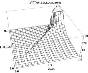
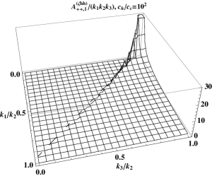
Figure 1: $\mathcal{A}_{++,1}^{(\zeta hh)}(k_{1}k_{2}k_{3})^{-1}$ as a function of $k_{1}/k_{2}$ and $k_{3}/k_{2}$ for $c_{h}/c_{s}=0.01$ in (a) and $c_{h}/c_{s}=10^{2}$ in (b), normalized to unity for $k_{1}=k_{2}=k_{3}$.

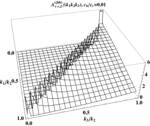
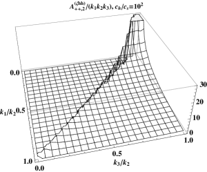
Figure 2: $\mathcal{A}_{++,2}^{(\zeta hh)}(k_{1}k_{2}k_{3})^{-1}$ as a function of $k_{1}/k_{2}$ and $k_{3}/k_{2}$ for $c_{h}/c_{s}=0.01$ in (a) and $c_{h}/c_{s}=10^{2}$ in (b), normalized to unity for $k_{1}=k_{2}=k_{3}$.

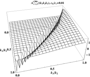
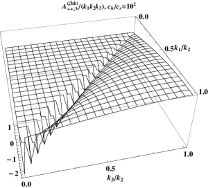
Figure 3: $\mathcal{A}_{++,3}^{(\zeta hh)}(k_{1}k_{2}k_{3})^{-1}$ as a function of $k_{1}/k_{2}$ and $k_{3}/k_{2}$ for $c_{h}/c_{s}=0.01$ in (a) and $c_{h}/c_{s}=10^{2}$ in (b), normalized to unity for $k_{1}=k_{2}=k_{3}$.

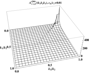
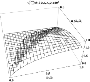
Figure 4: $\mathcal{A}_{++,4}^{(\zeta hh)}(k_{1}k_{2}k_{3})^{-1}$ as a function of $k_{1}/k_{2}$ and $k_{3}/k_{2}$ for $c_{h}/c_{s}=0.01$ in (a) and $c_{h}/c_{s}=10^{2}$ in (b), normalized to unity for $k_{1}=k_{2}=k_{3}$.

Let us discuss the shape of each cross bispectrum in momentum space. As shown in Ref. gw-non-g and also mentioned in the previous subsection, for the bispectrum of the tensor mode, ${\widetilde{\mathcal{A}}}_{({\rm new})}^{+++}$ and ${\widetilde{\mathcal{A}}}_{({\rm GR})}^{+++}$ have respectively peaks in the equilateral and squeezed limits. The shape of the bispectrum of scalar perturbations was also discussed in Ref. Gao:2011qe ; DeFelice:2011uc and the authors have found that it is well approximated by the equilateral shape.

In a similar way to the auto bispectra of tensors and scalars, we can also discuss the shapes of the cross bispectra of tensors and scalars in momentum space. However, contrary to the auto-bispectra of tensors and scalars, the shapes of cross bispectra strongly depend on the sound speeds of the tensor and scalar perturbations, as can be seen in Eqs. (92) and (101). Here, we denote a term proportional to $b_{q}$ in $\mathcal{A}_{s_{2},s_{3}}^{(\zeta hh)}$ as $\mathcal{A}_{s_{2},s_{3},q}^{(\zeta hh)}$ and also a term proportional to $c_{q}$ in $\mathcal{A}_{s}^{(\zeta\zeta h)}$ as $\mathcal{A}_{s,q}^{(\zeta\zeta h)}$.The shape of $\mathcal{A}_{++,1}^{(\zeta hh)}(k_{1}k_{2}k_{3})^{-1}$ in $k$-space for two limiting cases is plotted in Fig. 1. The left panel (a) and the right one (b) are respectively for the cases with $c_{h}/c_{s}=0.01$ and $c_{h}/c_{s}=10^{2}$. This figure implies that $\mathcal{A}_{++,1}^{(\zeta hh)}(k_{1}k_{2}k_{3})^{-1}$ has a peak in the squeezed limit ($k_{1}\ll k_{2}\sim k_{3}$) for both limiting cases. However, the sharpness of the peak seems to depend on the value of $c_{h}/c_{s}$. In Fig. 2 where $\mathcal{A}_{++,2}^{(\zeta hh)}(k_{1}k_{2}k_{3})^{-1}$ is plotted, we find that $\mathcal{A}_{++,2}^{(\zeta hh)}(k_{1}k_{2}k_{3})^{-1}$ for the case with $c_{h}/c_{s}=0.01$ has a sharp peak in the squeezed limit together with a non-trivial shape in wide region of the momentum space. For the case with $c_{h}/c_{s}=10^{2}$ (shown in Fig. 2-(b)), $\mathcal{A}_{++,2}^{(\zeta hh)}(k_{1}k_{2}k_{3})^{-1}$ also has a peak in the squeezed limit.

Contrary to $\mathcal{A}_{++,1}^{(\zeta hh)}(k_{1}k_{2}k_{3})^{-1}$ and $\mathcal{A}_{++,2}^{(\zeta hh)}(k_{1}k_{2}k_{3})^{-1}$, both of which have a peak in the squeezed limit, $\mathcal{A}_{++,3}^{(\zeta hh)}(k_{1}k_{2}k_{3})^{-1}$ does not have any sharp peak, but its shape strongly depends on the value of $c_{h}/c_{s}$, as shown in Fig. 3. In the case with $c_{h}/c_{s}\ll 1$, $\mathcal{A}_{++,3}^{(\zeta hh)}(k_{1}k_{2}k_{3})^{-1}$ becomes large at $k_{1}\ll k_{2}$, and then its shape looks to come close to so-called orthogonal type in the limit of $c_{h}/c_{s}\gg 1$. $\mathcal{A}_{++,4}^{(\zeta hh)}(k_{1}k_{2}k_{3})^{-1}$ also strongly depends on the value of $c_{h}/c_{s}$. As can be seen in Fig. 4, the peak of $\mathcal{A}_{++,4}^{(\zeta hh)}(k_{1}k_{2}k_{3})^{-1}$ shifts in the momentum space depending on $c_{h}/c_{s}$, and $\mathcal{A}_{++,4}^{(\zeta hh)}(k_{1}k_{2}k_{3})^{-1}$ for small $c_{h}$ has a finite value even in the squeezed limit. Although we do not show here, we also found that $\mathcal{A}_{++,5}^{(\zeta hh)}$, $\mathcal{A}_{++,6}^{(\zeta hh)}$ and $\mathcal{A}_{++,7}^{(\zeta hh)}$ have almost same shapes as $\mathcal{A}_{++,4}^{(\zeta hh)}$.

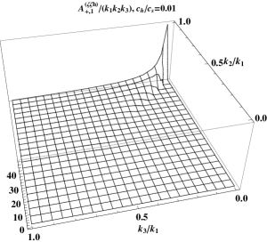
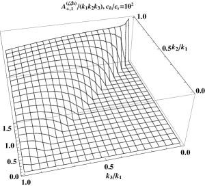
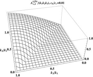
Figure 5: $\mathcal{A}_{+,q}^{(\zeta\zeta h)}(k_{1}k_{2}k_{3})^{-1}$ ((a) and (b) for $q=1$, and (c) and (d) for $q=2$) as a function of $k_{2}/k_{1}$ and $k_{3}/k_{1}$ for $c_{h}/c_{s}=0.01$ in (a) and (c), and $c_{h}/c_{s}=10^{2}$ in (b) and (d), normalized to unity for $k_{1}=k_{2}=k_{3}$.

In Fig. 5, $\mathcal{A}_{+,q}^{(\zeta\zeta h)}(k_{1}k_{2}k_{3})^{-1}$ for $q=1,2$ are plotted. This figure shows that $\mathcal{A}_{+,q}^{(\zeta\zeta h)}(k_{1}k_{2}k_{3})^{-1}$ also has strong dependence on $c_{h}/c_{s}$ and there is no divergence feature in the whole region of the momentum space, unlike the so-called local shape. Since we found $\mathcal{A}_{+,q}^{(\zeta\zeta h)}$ for $q=3,4,5,6$ have almost same shapes as $\mathcal{A}_{+,2}^{(\zeta\zeta h)}$, we do not show the plots for these contributions.

The detailed analysis of the shapes of the cross bispectra, including a precise comparison with the standard local-, equilateral and orthogonal shapes, is an issue in progress with the detailed analysis of CMB bispectra CMBbispectra .

V Examples

In this section, we consider two representative examples of inflation to estimate the amount of non-Gaussianities from tensor and scalar perturbations. The first example is general potential-driven inflation studied in Ref. GHiggs . This class of inflation models includes variants of Higgs inflation enabled by enhancing the effect of Hubble friction. These potential driven models have $c_{s}^{2}=\mathcal{O}(1)$ and $c_{h}^{2}\simeq 1$. Next, to see the impact of generic $c_{s}^{2}$ more clearly, we study k-inflation as another example.

V.1 The case of potential-driven inflation models

We wish to treat a wide class of potential-driven inflation models at one time. For this purpose, we introduce six $\phi$-dependent functions to write

$$K=-V(\phi)+\mathcal{K}(\phi)X,\quad G_{3}=h_{3}(\phi)X,\quad G_{4}=g(\phi)+h_{4}(\phi)X,\quad G_{5}=h_{5}(\phi)X.$$ (110)

In particular, the above form includes different Higgs inflation models proposed so far GHiggs . These may also be regarded as the Taylor expansion of $K(\phi,X)$ and $G_{i}(\phi,X)$ with respect to $X$. Would-be leading terms in $G_{3}$ and $G_{5}$ have been removed without loss of generality.

Slow-roll dynamics of general potential-driven inflation models has been addressed in Ref. GHiggs . During inflation we assume that the following slow-roll conditions are satisfied:

$$\epsilon=-\frac{\dot{H}}{H^{2}}\ll 1,\quad\eta=-\frac{\ddot{\phi}}{H\dot{\phi}}\ll 1,\quad\delta=\frac{\dot{g}}{Hg}\ll 1,\quad$$

$$\alpha_{2}=\frac{\dot{\mathcal{K}}}{H\mathcal{K}}\ll 1,\quad\alpha_{i}=\frac{\dot{h}_{i}}{Hh_{i}}\ll 1\;\;(i=3,4,5).$$ (111)

It is convenient to define

$$u(\phi):=\mathcal{K}+\frac{h_{4}V}{g},\quad v(\phi):=h_{3}+\frac{h_{5}V}{6g},\quad W(\phi):=\frac{1}{2}\left[u+\sqrt{u^{2}-4g^{2}v\frac{{\rm d}}{{\rm d}\phi}\left(\frac{V}{g^{2}}\right)}\right].$$ (112)

Under the slow-roll approximation the gravitational field equations reduce to

$$6gH^{2}\simeq V,\quad 2\epsilon+\delta\simeq\frac{X}{gH^{2}}\left(u+3H\dot{\phi}v\right).$$ (113)

Now it is easy to see that $\mathcal{F}_{T}\simeq\mathcal{G}_{T}\simeq 2g$ and

$$\mathcal{F}_{S}\simeq\frac{X}{H^{2}}\left(u+4H\dot{\phi}v\right)\simeq\frac{g}{3}(2\epsilon+\delta)\left(4-\frac{u}{W}\right),\quad$$

$$\mathcal{G}_{S}\simeq\frac{X}{H^{2}}\left(u+6H\dot{\phi}v\right)\simeq g(2\epsilon+\delta)\left(2-\frac{u}{W}\right),$$ (114)

so that $\mathcal{F}_{S}$ and $\mathcal{G}_{S}$ are slow-roll suppressed. It can also be seen that $c_{h}^{2}\simeq 1$ and $c_{s}^{2}=\mathcal{O}(1)$.

The coefficients of the cubic terms are given by

$$b_{1}\simeq\frac{Xu}{8H^{2}},\quad b_{2}\simeq\frac{g}{24}(2\epsilon+\delta)\left(4-\frac{u}{W}\right),\quad b_{3}\simeq-\frac{g}{4}(2\epsilon+\delta)\left(2-\frac{u}{W}\right),$$

$$b_{4}\simeq-\mu,\quad b_{5}\simeq-\frac{\mu}{6H}\frac{1-u/W}{2-u/W},\quad b_{7}\simeq\frac{\mu}{2H},\quad E_{shh}\simeq\frac{1}{4H}\zeta\dot{h}_{ij}E_{ij}^{h},$$ (115)

and

$$c_{1}\simeq\frac{g}{3}(2\epsilon+\delta)\left(4-\frac{u}{W}\right),\quad c_{2}\simeq\frac{g}{12H}(2\epsilon+\delta)\left(1-\frac{u}{W}\right)+\frac{\dot{\phi}X}{4H^{2}}\left(3h_{3}-\frac{h_{5}V}{6g}\right),\quad$$

$$c_{5}\simeq\mu,\bar{f}_{i}\simeq\frac{1}{2H}\zeta_{,j}h_{ij}\quad\bar{f}_{ij}\simeq-\frac{1}{4a^{2}H^{2}}\zeta_{,i}\zeta_{,j},$$ (116)

where $\mu=\dot{\phi}Xh_{5}$ as defined in (38). It turns out that the other coefficients are of higher order in the slow-roll parameter: $b_{6}\sim c_{3}\sim c_{4}\sim c_{6}=\mathcal{O}(\epsilon^{2})$.

V.2 The case of k-inflation

To extract the effect of the nontrivial sound speed, let us consider k-inflation, which is the simplest model with a generic value of $c_{s}^{2}$. In the case of k-inflation, $K=K(\phi,X)$, $G_{4}=M_{\rm Pl}^{2}/2$, $G_{3}=0=G_{5}$, we have

$$\mathcal{F}_{T}=\mathcal{G}_{T}=\Gamma=M_{\rm Pl}^{2},\quad\mathcal{F}_{S}=M_{\rm Pl}^{2}\epsilon,\quad\mathcal{G}_{S}=\frac{M_{\rm Pl}^{2}\epsilon}{c_{s}^{2}},\quad\Theta=M_{\rm Pl}^{2}H,\quad\mu=0,$$ (117)

with $c_{h}=1$ and $r=16\epsilon c_{s}$, which simplifies the coefficients in the cubic Lagrangians:

$$b_{1}=b_{2}=\frac{M_{\rm Pl}^{2}\epsilon}{8},\quad b_{3}=-\frac{M_{\rm Pl}^{2}\epsilon}{4c_{s}^{2}},\quad b_{4}=b_{5}=b_{6}=b_{7}=0,\quad$$

$$E_{shh}=\frac{1}{4H}\zeta\dot{h}_{ij}E_{ij}^{h},$$ (118)

$$c_{1}=M_{\rm Pl}^{2}\epsilon,\quad c_{2}=0,\quad c_{3}=\frac{M_{\rm Pl}^{2}\epsilon^{2}}{2c_{s}^{2}},\quad c_{4}=c_{5}=0,\quad c_{6}=\frac{M_{\rm Pl}^{2}\epsilon^{2}}{4c_{s}^{4}},$$ (119)

$$\bar{f}_{i}=\frac{1}{2H}\zeta_{,j}h_{ij},\quad\bar{f}_{ij}=\frac{\epsilon}{2Hc_{s}^{2}}\zeta_{,i}\psi_{,j}-\frac{1}{4a^{2}H^{2}}\zeta_{,i}\zeta_{,j}.$$ (120)

Note that in deriving the above coefficients we have not invoked the slow-roll expansion.

VI Discussion

In this paper we have presented the full bispectra, including the cross bispectra of the primordial curvature and tensor perturbations, in the generalized G-inflation model which is the most general single-field inflation model with the second order equations of motion.

In the event full observations of these quantities could be made, we could extract many pieces of interesting information on the underlying theory. For example, by observing three-point tensor correlation function, we can in principle determine the kinetic coupling to the Einstein tensor through $\mu$. Another interesting quantity is the cross bispectrum of two tensors and one scalar. If we could observationally identify their coefficients $b_{2},~{}b_{3}$ and $b_{6}$, we could in principle determine $\mathcal{F}_{S}$, $\mathcal{G}_{S}$, $\mathcal{F}_{T}$, and $\mathcal{G}_{T}$ independently with the help of the three-tensor bispectrum which would provide a consistency relation of the theory for the tensor-to-scalar ratio (36).

Let us next turn to two-scalar and one-tensor bispectrum whose effective Lagrangian is given by (53). Its most interesting component is the first term proportional to $c_{1}=\mathcal{F}_{S}$ which could be singled out by taking $k_{3}$ small. In the standard canonical inflation as well as in k-inflation, the coefficient simply takes $\displaystyle{c_{1}=\mathcal{F}_{S}=M_{\rm Pl}^{2}\epsilon=\frac{M_{\rm Pl}^{2}r}{16c_{s}}}$ as derived in (119), where we have used the consistency relation in the last equality.

We can also show that this feature remains valid in the case where a sizable local non-Gaussianity is generated as in the cases of the curvaton scenario Lyth:2002my and the modulated reheating scenarios Zaldarriaga:2003my . In such case curvature perturbation $\zeta$ is sourced by another scalar field which we denote by $\sigma$ and its fluctuation by $\delta\sigma$. One can relate $\zeta$ and $\delta\sigma$ as

$$\zeta=N_{\sigma}(\sigma)\delta\sigma+\frac{1}{2}N_{\sigma\sigma}(\sigma)(\delta\sigma)^{2},$$ (121)

using the $\delta N$-formalism Starobinsky:1986fxa . Suppose that $\sigma$ has the Lagrangian $\mathcal{L}_{\sigma}=\kappa(Y,\sigma)$ with $Y:=-(\partial\sigma)^{2}/2$. Since the dynamics of $\sigma$ is practically frozen during inflation and it practically behaves as a massless minimally-coupled field, one can expand $\mathcal{L}_{\sigma}=\kappa(0,\sigma_{0})+\kappa_{\sigma}(0,\sigma_{0})Y$ in this regime where $\sigma_{0}$ is its expectation value in the domain including our horizon today. Then the mean-square fluctuation amplitude of $\sigma$ is given by

$$\langle(\delta\sigma)^{2}\rangle=\frac{H^{2}}{4\pi^{2}\kappa_{\sigma}(0,\sigma_{0})}=\frac{1}{N_{\sigma}^{2}(\sigma_{0})}\mathcal{P}_{\zeta},$$ (122)

the latter being an outcome of (121), and it determines the relation between $\delta\sigma$ and $\zeta$, too. Then the effective Lagrangian representing tensor-scalar-scalar coupling is generated from the kinetic term of $\sigma$ in this case and reads

$$\mathcal{L}_{ssh}=\frac{1}{2}\kappa_{\sigma}(0,\sigma_{0})h^{\mu\nu}\sigma_{,\mu}\sigma_{,\nu}=\frac{1}{2}\left(\frac{H}{2\pi}\right)^{2}\mathcal{P}_{\zeta}h^{\mu\nu}\zeta_{,\mu}\zeta_{,\nu}=\frac{M_{\rm Pl}^{2}r}{16}h_{ij}\zeta_{,i}\zeta_{,j}.$$ (123)

Note that in this case the sound speed is equal to unity. Thus we find that if the sector responsible for the generation of curvature perturbations is minimally coupled to gravity with no extra Galileon-like terms, $c_{1}$ takes the same form whether they are generated by the inflaton or another scalar field. Thus this term can provide a test of the generalized Galileon as a source of the structure of the Universe.

It is a non-trivial issue how to normalize the cross bispectra. In this paper, we have normalized them by the power spectrum of the curvature perturbation. This is mainly because these cross bispectra generate the auto- and the cross-bispectra of the temperature fluctuation and the E-mode polarization, which are mainly sourced by the curvature perturbation. However, such a normalization may be inadequate for the cross bispectra including the B-mode polarization. Therefore, we need to directly investigate the impacts on the CMB bispectra and it is interesting to see the CMB cross-bispectra between the temperature fluctuations and B-mode polarizations which are sourced directly from the primordial cross-bispectra of the scalar and the tensor modes Shiraishi:2010kd ; Shiraishi:2011st . Constraining the model parameters by CMB bispectra is a work in progress CMBbispectra .

References

• (1) K. Sato, Mon. Not. Roy. Astron. Soc.  195, 467 (1981); A. H. Guth, Phys. Rev.  D 23, 347 (1981).
• (2) A. A. Starobinsky, Phys. Lett.  B 91, 99 (1980).
• (3) [Planck Collaboration], astro-ph/0604069.
• (4) D. Baumann et al. [CMBPol Study Team Collaboration], AIP Conf. Proc.  1141, 10 (2009) [arXiv:0811.3919 [astro-ph]].
• (5) http://cmbpol.kek.jp/litebird/documents.html
• (6) N. Kaisar Mon. Not. Roy. Astron. Soc. 202, 1169 (1983); A.G. Polnarev, Soviet Astronomy, 29, 607 (1985); J.R. Bond and G. Efstathiou, Mon. Not. Roy. Astron. Soc. 226, 655 (1987); R. A. Frewin, A. G. Polnarev and P. Coles, Mon. Not. Roy. Astron. Soc.  266, L21 (1994); R. Crittenden, R. L. Davis and P. J. Steinhardt, Astrophys. J.  417, L13 (1993); R. Crittenden, J. R. Bond, R. L. Davis, G. Efstathiou and P. J. Steinhardt, Phys. Rev. Lett.  71, 324 (1993).
• (7) M. Zaldarriaga and U. Seljak, Phys. Rev. D 55, 1830 (1997) [astro-ph/9609170]; U. Seljak and M. Zaldarriaga, Phys. Rev. Lett.  78, 2054 (1997) [astro-ph/9609169].
• (8) A. D. Linde, Phys. Lett.  B 108, 389 (1982); A. Albrecht and P. J. Steinhardt, Phys. Rev. Lett.  48, 1220 (1982); A. D. Linde, Phys. Lett.  B 129, 177 (1983).
• (9) J. M. Maldacena, JHEP 0305, 013 (2003) [astro-ph/0210603].
• (10) C. Armendariz-Picon, T. Damour and V. F. Mukhanov, Phys. Lett. B 458, 209 (1999) [hep-th/9904075]; J. Garriga and V. F. Mukhanov, Phys. Lett. B 458, 219 (1999) [hep-th/9904176].
• (11) E. Silverstein and D. Tong, Phys. Rev. D 70, 103505 (2004) [hep-th/0310221].
• (12) N. Arkani-Hamed, P. Creminelli, S. Mukohyama and M. Zaldarriaga, JCAP 0404, 001 (2004) [hep-th/0312100].
• (13) T. Kobayashi, M. Yamaguchi and J. Yokoyama, Phys. Rev. Lett.  105, 231302 (2010) [arXiv:1008.0603 [hep-th]]; C. Burrage, C. de Rham, D. Seery and A. J. Tolley, JCAP 1101, 014 (2011) [arXiv:1009.2497 [hep-th]].
• (14) D. Seery and J. E. Lidsey, JCAP 0506, 003 (2005) [astro-ph/0503692]; X. Chen, M. -x. Huang, S. Kachru and G. Shiu, JCAP 0701, 002 (2007) [hep-th/0605045].
• (15) M. Alishahiha, E. Silverstein and D. Tong, Phys. Rev. D 70, 123505 (2004) [hep-th/0404084].
• (16) S. Mizuno, K. Koyama, Phys. Rev.  D82, 103518 (2010). [arXiv:1009.0677 [hep-th]]; A. De Felice and S. Tsujikawa, JCAP 1104, 029 (2011) [arXiv:1103.1172 [astro-ph.CO]]; T. Kobayashi, M. Yamaguchi and J. Yokoyama, Phys. Rev. D 83, 103524 (2011) [arXiv:1103.1740 [hep-th]].
• (17) M. Shiraishi, D. Nitta, S. Yokoyama, K. Ichiki and K. Takahashi, Prog. Theor. Phys.  125, 795 (2011) [arXiv:1012.1079 [astro-ph.CO]].
• (18) P. McFadden and K. Skenderis, JCAP 1106, 030 (2011) [arXiv:1104.3894 [hep-th]]; A. Bzowski, P. McFadden and K. Skenderis, JHEP 1203, 091 (2012) [arXiv:1112.1967 [hep-th]].
• (19) D. Seery, M. S. Sloth and F. Vernizzi, JCAP 0903, 018 (2009) [arXiv:0811.3934 [astro-ph]].
• (20) N. Bartolo, E. Dimastrogiovanni and A. Vallinotto, JCAP 1011, 003 (2010) [arXiv:1006.0196 [astro-ph.CO]].
• (21) R. R. Caldwell, L. Motta and M. Kamionkowski, Phys. Rev. D 84, 123525 (2011) [arXiv:1109.4415 [astro-ph.CO]]; L. Motta and R. R. Caldwell, arXiv:1203.1033 [astro-ph.CO].
• (22) T. Kobayashi, M. Yamaguchi and J. Yokoyama, Prog. Theor. Phys.  126, 511 (2011) [arXiv:1105.5723 [hep-th]].
• (23) G. W. Horndeski, Int. J. Theor. Phys. 10 (1974) 363-384.
• (24) C. Deffayet, X. Gao, D. A. Steer and G. Zahariade, Phys. Rev. D 84, 064039 (2011) [arXiv:1103.3260 [hep-th]].
• (25) C. Charmousis, E. J. Copeland, A. Padilla and P. M. Saffin, Phys. Rev. Lett.  108, 051101 (2012) [arXiv:1106.2000 [hep-th]].
• (26) B. L. Spokoiny, Phys. Lett.  B 147, 39 (1984); T. Futamase and K. -i. Maeda, Phys. Rev. D 39, 399 (1989); D. S. Salopek, J. R. Bond and J. M. Bardeen, Phys. Rev.  D 40, 1753 (1989); R. Fakir and W. G. Unruh, Phys. Rev.  D 41, 1783 (1990); D. I. Kaiser, Phys. Rev.  D 52, 4295 (1995) [arXiv:astro-ph/9408044]; N. Makino and M. Sasaki, Prog. Theor. Phys.  86, 103 (1991).
• (27) J. L. Cervantes-Cota and H. Dehnen, Nucl. Phys. B 442, 391 (1995) [astro-ph/9505069]; F. L. Bezrukov, A. Magnin and M. Shaposhnikov, Phys. Lett.  B 675, 88 (2009) [arXiv:0812.4950 [hep-ph]]; F. Bezrukov and M. Shaposhnikov, JHEP 0907, 089 (2009) [arXiv:0904.1537 [hep-ph]]; A. O. Barvinsky, A. Y. Kamenshchik, C. Kiefer, A. A. Starobinsky and C. Steinwachs, JCAP 0912, 003 (2009) [arXiv:0904.1698 [hep-ph]]; A. O. Barvinsky, A. Y. .Kamenshchik, C. Kiefer, A. A. Starobinsky and C. F. Steinwachs, arXiv:0910.1041 [hep-ph]; F. Bezrukov, A. Magnin, M. Shaposhnikov and S. Sibiryakov, arXiv:1008.5157 [hep-ph].
• (28) D. La and P. J. Steinhardt, Phys. Rev. Lett.  62, 376 (1989) [Erratum-ibid.  62, 1066 (1989)].
• (29) M. B. Mijic, M. S. Morris, W. -M. Suen, Phys. Rev.  D34, 2934 (1986).
• (30) C. Germani, A. Kehagias, Phys. Rev. Lett.  105, 011302 (2010) [arXiv:1003.2635 [hep-ph]].
• (31) X. Gao and D. A. Steer, JCAP 1112, 019 (2011) [arXiv:1107.2642 [astro-ph.CO]].
• (32) A. De Felice and S. Tsujikawa, Phys. Rev. D 84, 083504 (2011) [arXiv:1107.3917 [gr-qc]].
• (33) S. Renaux-Petel, JCAP 1202, 020 (2012) [arXiv:1107.5020 [astro-ph.CO]].
• (34) R. H. Ribeiro, JCAP 1205, 037 (2012) [arXiv:1202.4453 [astro-ph.CO]].
• (35) X. Gao, T. Kobayashi, M. Yamaguchi and J. Yokoyama, Phys. Rev. Lett.  107, 211301 (2011) [arXiv:1108.3513 [astro-ph.CO]].
• (36) A. Nicolis, R. Rattazzi, E. Trincherini, Phys. Rev.  D79, 064036 (2009) [arXiv:0811.2197 [hep-th]].
• (37) C. Deffayet, G. Esposito-Farese, A. Vikman, Phys. Rev.  D79, 084003 (2009) [arXiv:0901.1314 [hep-th]].
• (38) X. Gao, JCAP 1110, 021 (2011) [arXiv:1106.0292 [astro-ph.CO]].
• (39) A. Adams, N. Arkani-Hamed, S. Dubovsky, A. Nicolis and R. Rattazzi, JHEP 0610, 014 (2006) [hep-th/0602178].
• (40) E. Babichev, V. Mukhanov and A. Vikman, JHEP 0802, 101 (2008) [arXiv:0708.0561 [hep-th]].
• (41) L. Lorenz, J. Martin and C. Ringeval, Phys. Rev. D 78, 083513 (2008) [arXiv:0807.3037 [astro-ph]].
• (42) J. Khoury and F. Piazza, JCAP 0907, 026 (2009) [arXiv:0811.3633 [hep-th]]. J. Noller and J. Magueijo, Phys. Rev. D 83, 103511 (2011) [arXiv:1102.0275 [astro-ph.CO]].
• (43) K. Kamada, T. Kobayashi, T. Takahashi, M. Yamaguchi and J. Yokoyama, arXiv:1203.4059 [hep-ph].
• (44) D. H. Lyth, C. Ungarelli and D. Wands, Phys. Rev. D 67, 023503 (2003) [astro-ph/0208055]; M. Sasaki, J. Valiviita and D. Wands, Phys. Rev. D 74, 103003 (2006) [astro-ph/0607627].
• (45) M. Zaldarriaga, Phys. Rev. D 69, 043508 (2004) [astro-ph/0306006]; T. Suyama and M. Yamaguchi, Phys. Rev. D 77, 023505 (2008) [arXiv:0709.2545 [astro-ph]].
• (46) A. A. Starobinsky, JETP Lett.  42 (1985) 152 [Pisma Zh. Eksp. Teor. Fiz.  42 (1985) 124]; Y. Nambu and A. Taruya, Class. Quant. Grav.  13, 705 (1996) [arXiv:astro-ph/9411013]; M. Sasaki and E. D. Stewart, Prog. Theor. Phys.  95, 71 (1996) [arXiv:astro-ph/9507001].
• (47) M. Shiraishi, D. Nitta and S. Yokoyama, Prog. Theor. Phys.  126, 937 (2011) [arXiv:1108.0175 [astro-ph.CO]].
• (48) X. Gao, T. Kobayashi, M. Shiraishi, M. Yamaguchi, J. Yokoyama, and S. Yokoyama, in preparation.