Fast shape reconstruction of perfectly conducting cracks by using a multi-frequency topological derivative strategy

Abstract

This paper concerns a fast, one-step iterative technique of imaging extended perfectly conducting cracks with Dirichlet boundary condition. In order to reconstruct the shape of cracks from scattered field data measured at the boundary, we introduce a topological derivative-based electromagnetic imaging function operated at several nonzero frequencies. The properties of the imaging function are carefully analyzed for the configurations of both symmetric and non-symmetric incident field directions. This analysis explains why the application of incident fields with symmetric direction operated at multiple frequencies guarantees a successful reconstruction. Various numerical simulations with noise-corrupted data are conducted to assess the performance, effectiveness, robustness, and limitations of the proposed technique.

1 Introduction

One goal of the inverse scattering problem is to find the shape of bulk or flaw in a medium using the scattered field data measured at the boundary. This is an old but it has several of applications such as detection of cracks in material engineering, ultrasound imaging in medical sciences, and scanning anti-personnel mines hidden in the ground in military services. Related researches may be found in [3, 7, 16, 17, 18, 37] and the references therein. In many studies, various shape reconstruction algorithms have been developed, most of which are focused on the minimization of the least-square functional by using a Newton-type iteration strategy, e.g., level-set method [2, 18, 35]. The merits of the iteration strategy is that it does not require a very large number of boundary measurements for complete shape reconstruction; instead, in order to guarantee successful reconstruction, it demands very high computational expenditures, optimal regularization terms related to the problems at hand, calculation of a complex Fréchet derivative at each iteration, and a priori information of the unknown target to be reconstructed. Nevertheless, even if these conditions are satisfied, the iteration strategy must begin with an initial guess that is close to the true one in order to avoid undesirable situations such as non-convergence or falling into the local minima. Therefore, development of a mathematical theory and an algorithm for generating a good initial guess is an important research topic.

Conversely, certain non-iterative shape reconstruction algorithms have been proposed; for example, MUltiple SIgnal Classification (MUSIC) algorithm [6, 10, 32, 34], linear sampling method [15, 21], Kirchhoff migration [6, 28, 29, 33], and Fourier inversion based one [8, 9, 11]. In contrast with the iterative strategy, these algorithms require a large amount of incident field data and a significant number of boundary measurements. However, if these conditions are satisfied, non-iterative shape reconstruction algorithms can prove to be effective, fast, and easy to extend to multiple targets.

Topological derivative concept is a non-iterative strategy. This concept was originally developed for the shape optimization problem, but its application to rapid shape reconstruction has only recently been proven. Related works can be found in [5, 10, 12, 13, 14, 24, 25, 27, 30, 31, 38] and references therein. One of the advantages of topological derivative concept is that it does not require a large amount of many incident field data; however, a reduction in the amount of this data has been reported to result in poor resolution of the reconstructed shape.

The purpose of this literature is to establish an effective and fast reconstruction algorithm for detecting both the location and shape of perfectly conducting crack(s) from boundary-measured scattered field data by using only a small amount of incident field data. Based on the structure of topological derivative imaging functional operated at a fixed-frequency [24] and multi-frequency imaging schemes [6, 26], we introduce a multi-frequency topological derivative concept. Note that recent work [4, Formula (1.33)] has briefly introduced a multi-frequency topological derivative but through a more detailed analysis, we investigate the structure of the proposed multi-frequency topological derivative and its benefits over the traditional topological derivative.

The remainder of this paper is organized as follows. Section 2 briefly introduces the traditional topological derivative by creating a linear, narrow crack. Section 3 describes the design of a multi-frequency topological derivative imaging function and analyzes it to investigate its properties. Section 4 presents various numerical experiments to assess the performance of the proposed imaging function under various situations. Section 5 contains a short conclusion and some remarks on future work.

2 Topological derivative: an inspection

Assume that a perfectly conducting crack $\mathcal{C}$ is completely hidden in a homogeneous domain $\mathcal{D}\subset\mathbb{R}^{2}$ with a smooth boundary $\mathcal{B}$. We denote $\vec{x}_{c}$ as a two-dimensional vector that lies on crack $\mathcal{C}$.

Throughout this paper, we consider the so-called Transverse Magnetic (TM) polarization case, letting $u_{m}^{\mathrm{total}}(\vec{x};k)$ be the (single-component) electric field that satisfies the following boundary value problem:

$$\left\{\begin{array}[]{rcl}\Delta u_{m}^{\mathrm{total}}(\vec{x};k)+k^{2}u_{m}^{\mathrm{total}}(\vec{x};k)=0&\mbox{in}&\mathcal{D}\backslash\overline{\mathcal{C}}\\ \vskip 6.0pt plus 2.0pt minus 2.0pt\cr u_{m}^{\mathrm{total}}(\vec{x};k)=0&\mbox{on}&\mathcal{C}\\ \vskip 6.0pt plus 2.0pt minus 2.0pt\cr\displaystyle\frac{\partial u_{m}^{\mathrm{total}}(\vec{x};k)}{\partial\vec{\nu}(\vec{x})}=\frac{\partial\exp(ik\vec{\theta}_{m}\cdot\vec{x})}{\partial\vec{\nu}(\vec{x})}&\mbox{on}&\mathcal{B},\end{array}\right.$$ (1)

where $\vec{\nu}(\vec{x})$ represents the unit outward normal to $\vec{x}\in\mathcal{B}$ and $\vec{\theta}_{m}$, $m=1,2,\cdots,M$, denotes the two-dimensional vector on the unit circle $\mathcal{S}^{1}$. Throughout this paper, we let $k$ denote a strictly positive wavenumber and presume $k^{2}$ to not be an eigenvalue of (1). Similarly, let $u_{m}^{\mathrm{back}}(\vec{x};k)=\exp(ik\vec{\theta}_{m}\cdot\vec{x})$ be the solution of equation (1) without $\mathcal{C}$. Then, the problem we consider here is the computation of the topological derivative of the residual function depending on the solution $u_{m}^{\mathrm{total}}(\vec{x};k)$:

$$\mathbb{R}(\mathcal{D};k):=\frac{1}{2}\sum_{m=1}^{M}\left|\left|u_{m}^{\mathrm{total}}(\vec{x};k)-u_{m}^{\mathrm{back}}(\vec{x};k)\right|\right|_{L^{2}(\mathcal{B})}^{2}=\frac{1}{2}\sum_{m=1}^{M}\int_{\mathcal{B}}\left|u_{m}^{\mathrm{total}}(\vec{x};k)-u_{m}^{\mathrm{back}}(\vec{x};k)\right|^{2}d\mathcal{B}(\vec{x}),$$ (2)

where $|u_{m}^{\mathrm{total}}(\vec{x};k)|^{2}=u_{m}^{\mathrm{total}}(\vec{x};k)\overline{u_{m}^{\mathrm{total}}(\vec{x};k)}$.

In order to compute the topological derivative, let us create a small linear crack $\mathcal{L}$ of length $2\ell(\ll k)$ centered at $\vec{x}_{s}=(x_{s}^{1},x_{s}^{2})\in\mathcal{D}\backslash\mathcal{B}$ such that

$$\mathcal{L}=\left\{(\xi,x_{s}^{2}):x_{s}^{1}-\ell\leq\xi\leq x_{s}^{1}+\ell\right\},$$

and denote $\mathcal{D}\vee\mathcal{L}$ as that domain. Then, because of the change in the topology of $\mathcal{D}$, we can consider the topological derivative $\mathbb{R}_{\mathrm{TD}}(\vec{x}_{s};k)$ based on the residual function $\mathbb{R}(\mathcal{D};k)$ with respect to point $\vec{x}_{s}$ as follows:

$$\mathbb{R}_{\mathrm{TD}}(\vec{x}_{s};k)=\lim_{\ell\to 0+}\frac{\mathbb{R}(\mathcal{D}\vee\mathcal{L};k)-\mathbb{R}(\mathcal{D};k)}{\phi(\ell;k)},$$ (3)

where $\phi(\ell;k)\longrightarrow 0$ as $\ell\longrightarrow 0+$. From relationship (3), we have the following asymptotic expansion:

$$\mathbb{R}(\mathcal{D}\vee\mathcal{L};k)=\mathbb{R}(\mathcal{D};k)+\phi(\ell;k)\mathbb{R}_{\mathrm{TD}}(\vec{x}_{s};k)+o(\phi(\ell;k)).$$

Then, the topological derivative $\mathbb{R}_{\mathrm{TD}}(\vec{x}_{s};k)$ with $M$ different incident waves at a given wavenumber $k$ is as follows (see [24] for its derivation).

Lemma 2.1 (Topological derivative)

Let $\Re(f)$ denote the real part of $f$. Then, the topological derivative corresponding to (2) is given by

$$\mathbb{R}_{\mathrm{TD}}(\vec{x}_{s};k)=\Re\left[\sum_{m=1}^{M}v_{m}^{\mathrm{adjnt}}(\vec{x}_{s};k)\overline{u_{m}^{\mathrm{back}}(\vec{x}_{s};k)}\right],$$ (4)

where $v_{m}^{\mathrm{adjnt}}(\cdot;k)$ satisfies the following adjoint problem:

$$\left\{\begin{array}[]{rcl}\displaystyle\Delta v_{m}^{\mathrm{adjnt}}(\vec{x};k)+k^{2}v_{m}^{\mathrm{adjnt}}(\vec{x};k)=0&\mbox{in}&\mathcal{D}\\ \vskip 6.0pt plus 2.0pt minus 2.0pt\cr\displaystyle\frac{\partial v_{m}^{\mathrm{adjnt}}(\vec{x};k)}{\partial\vec{\nu}(\vec{x})}=u_{m}^{\mathrm{total}}(\vec{x};k)-u_{m}^{\mathrm{back}}(\vec{x};k)&\mbox{on}&\mathcal{B}\end{array}\right.$$ (5)

3 Multi-frequency topological derivative: introduction and analysis

In this section, we introduce a multi-frequency topological derivative imaging function and explore its properties. Based on recent research [5, 10, 30, 31], a sufficiently large number of incident directions are required to obtain a good result. This means that if $M$ is small, an image with poor resolution will be reconstructed. Moreover, when boundary measurement data are affected by a large amount of random noise, (4) will fail to reconstruct a good image. Inspired by multi-frequency imaging algorithms [6, 28, 29, 33], we consider the following multi-frequency topological derivative for several wavenumbers $\{k_{f}:f=1,2,\cdots,F\}$:

$$\mathbb{R}_{\mathrm{MTD}}(\vec{x}_{s};F)=\frac{1}{F}\sum_{f=1}^{F}\frac{\mathbb{R}_{\mathrm{TD}}(\vec{x}_{s};k_{f})}{\displaystyle\max_{\vec{x}_{s}\in\mathcal{D}}|\mathbb{R}_{\mathrm{TD}}(\vec{x}_{s};k_{f})|},$$ (6)

where $\mathbb{R}_{\mathrm{TD}}(\vec{x}_{s};k_{f})$ is given by (4) for $k=k_{f}$, $f=1,2,\cdots,F$.

In this section, we investigate the structure of (6). For this purpose, we recall a useful result (see [24]) as follows.

Lemma 3.2

Let $A\sim B$ imply that there exists a constant $C$ such that $A=BC$. Then, for $\vec{x}_{s}\in\mathcal{D}$ and $\vec{x}_{c}\in\mathcal{C}$, (4) satisfies

$$\mathbb{R}_{\mathrm{TD}}(\vec{x}_{s};k)\sim\Re\left[\frac{i}{k}\sum_{m=1}^{M}\exp(ik\vec{\theta}_{m}\cdot(\vec{x}_{c}-\vec{x}_{s}))\Phi(\vec{x}_{c},\vec{x}_{s};k)\right].$$ (7)

Here $\Phi(x,y;k)$ denotes the two-dimensional time-harmonic fundamental solution (or Green’s function) of Helmholtz equation

$$\Phi(x,y;k)=-\frac{i}{4}H_{0}^{1}(k|x-y|)=-\frac{i}{4}\bigg{(}J_{0}(k|x-y|)+iY_{0}(k|x-y|)\bigg{)},$$

where $H_{0}^{1}$, $J_{0}$, and $Y_{0}$ denote the Hankel function of the first kind, Bessel function, and Neumann function of order zero, respectively.

Consequently, (6) is analyzed for the following three cases of interest.

Theorem 3.3 (Case 1: Symmetric incident directions)

Under the configuration of a small number of symmetric incident directions, the structure of (6) is

$$\mathbb{R}_{\mathrm{MTD}}(\vec{x}_{s};F)\sim\sum_{m=1}^{M}\frac{1}{\displaystyle|\vec{x}_{c}-\vec{x}_{s}|\sqrt{1-\bigg{(}\vec{\theta}_{m}\cdot\frac{\vec{x}_{c}-\vec{x}_{s}}{|\vec{x}_{c}-\vec{x}_{s}|}\bigg{)}^{2}}},$$

for a sufficiently large $F$ and $k_{F}\longrightarrow\infty$.

Proof 1

Assume that the symmetric incident directions are of the form:

$$\vec{\theta}_{m}:=\bigg{(}\cos\frac{2(m-1)\pi}{M},\sin\frac{2(m-1)\pi}{M}\bigg{)},\quad m=1,2,\cdots,M,$$

where $M$ is an even number, say, $M=2N$. Based on this form, $\vec{\theta}_{l}$ satisfies $\vec{\theta}_{l}=-\vec{\theta}_{l+N}$ for $l=1,2,\cdots,N$.

In contrast with Lemma 3.2, we assume that $M$ is not sufficiently large. Let $\Im(f)$ denote the imaginary part of $f$ then since

$$\Re\bigg{[}\exp(ik\vec{\theta}_{l}\cdot(\vec{x}_{c}-\vec{x}_{s}))\bigg{]} =\Re\bigg{[}\exp(ik\vec{\theta}_{l+N}\cdot(\vec{x}_{c}-\vec{x}_{s}))\bigg{]}$$

$$\Im\bigg{[}\exp(ik\vec{\theta}_{l}\cdot(\vec{x}_{c}-\vec{x}_{s}))\bigg{]} =-\Im\bigg{[}\exp(ik\vec{\theta}_{l+N}\cdot(\vec{x}_{c}-\vec{x}_{s}))\bigg{]},$$

(7) becomes

$$\mathbb{R}_{\mathrm{TD}}(\vec{x}_{s};k_{f}) \sim\Re\left[\frac{i}{k_{f}}\sum_{m=1}^{M}\exp(ik_{f}\vec{\theta}_{m}\cdot(\vec{x}_{c}-\vec{x}_{s}))\Phi(\vec{x}_{c},\vec{x}_{s};k_{f})\right]$$

$$=\Re\left[\frac{1}{2k_{f}}\sum_{m=1}^{N}\cos(k_{f}\vec{\theta}_{m}\cdot(\vec{x}_{c}-\vec{x}_{s}))\{J_{0}(k_{f}|\vec{x}_{c}-\vec{x}_{s}|)+iY_{0}(k_{f}|\vec{x}_{c}-\vec{x}_{s}|)\}\right]$$

$$=\frac{1}{2k_{f}}\sum_{m=1}^{N}\cos(k_{f}\vec{\theta}_{m}\cdot(\vec{x}_{c}-\vec{x}_{s}))J_{0}(k_{f}|\vec{x}_{c}-\vec{x}_{s}|).$$

Therefore,

$$\frac{\mathbb{R}_{\mathrm{TD}}(\vec{x}_{s};k_{f})}{\displaystyle\max_{\vec{x}_{s}\in\mathcal{D}}|\mathbb{R}_{\mathrm{TD}}(\vec{x}_{s};k_{f})|}\approx\frac{1}{N}\sum_{m=1}^{N}\cos(k_{f}\vec{\theta}_{m}\cdot(\vec{x}_{c}-\vec{x}_{s}))J_{0}(k_{f}|\vec{x}_{c}-\vec{x}_{s}|)$$

Let us recall that for $\Re(\mu)>-1$ (see [1, formula 11.4.37 (p. 487)])

$$\int_{0}^{\infty}\cos atJ_{\mu}(bt)dt=\left\{\begin{array}[]{ccc}\vskip 6.0pt plus 2.0pt minus 2.0pt\displaystyle\frac{1}{\sqrt{b^{2}-a^{2}}}\cos\bigg{(}\mu\sin^{-1}\frac{a}{b}\bigg{)}&\mbox{if}&0\leq b<a\\ \displaystyle-\frac{b^{\mu}}{\sqrt{a^{2}-b^{2}}(a+\sqrt{a^{2}-b^{2}})^{\mu}}\cos\bigg{(}\frac{\mu\pi}{2}\bigg{)}&\mbox{if}&0<a<b.\end{array}\right.$$

Let $a=\vec{\theta}_{m}\cdot(\vec{x}_{c}-\vec{x}_{s})$, $b=|\vec{x}_{c}-\vec{x}_{s}|$, and $\mu=0$. Then since

$$b^{2}-a^{2}=|\vec{x}_{c}-\vec{x}_{s}|^{2}\bigg{[}1-\bigg{(}\vec{\theta}_{m}\cdot\frac{\vec{x}_{c}-\vec{x}_{s}}{|\vec{x}_{c}-\vec{x}_{s}|}\bigg{)}^{2}\bigg{]}\geq 0,$$ (8)

by letting $k_{F}\longrightarrow\infty$, (6) becomes

$$\begin{aligned} \mathbb{R}_{\mathrm{MTD}}(\vec{x}_{s};F)&=\frac{1}{F}\sum_{f=1}^{F}\frac{\mathbb{R}_{\mathrm{TD}}(\vec{x}_{s};k_{f})}{\displaystyle\max_{\vec{x}_{s}\in\mathcal{D}}|\mathbb{R}_{\mathrm{TD}}(\vec{x}_{s};k_{f})|}\approx\frac{1}{N}\sum_{m=1}^{N}\int_{0}^{\infty}\cos(k\vec{\theta}_{m}\cdot(\vec{x}_{c}-\vec{x}_{s}))J_{0}(k|\vec{x}_{c}-\vec{x}_{s}|)dk\\ &=\frac{1}{N}\sum_{m=1}^{N}\frac{1}{\displaystyle|\vec{x}_{c}-\vec{x}_{s}|\sqrt{1-\bigg{(}\vec{\theta}_{m}\cdot\frac{\vec{x}_{c}-\vec{x}_{s}}{|\vec{x}_{c}-\vec{x}_{s}|}\bigg{)}^{2}}}.\end{aligned}$$ (9)

Theorem 3.4 (Case 2: Non-symmetric incident directions)

Under the configuration of a small number of non-symmetric incident directions, the structure of (6) becomes

$$\mathbb{R}_{\mathrm{MTD}}(\vec{x}_{s};F)\sim\sum_{m=1}^{M}\frac{\displaystyle 1-\frac{2}{\pi}\sin^{-1}\bigg{(}\vec{\theta}_{m}\cdot\frac{\vec{x}_{c}-\vec{x}_{s}}{|\vec{x}_{c}-\vec{x}_{s}|}\bigg{)}}{\displaystyle|\vec{x}_{c}-\vec{x}_{s}|\sqrt{1-\bigg{(}\vec{\theta}_{m}\cdot\frac{\vec{x}_{c}-\vec{x}_{s}}{|\vec{x}_{c}-\vec{x}_{s}|}\bigg{)}^{2}}},$$

for a sufficiently large $F$ and $k_{F}\longrightarrow\infty$.

Proof 2

In constrast with Theorem 3.3, we assume that the incident directions are non-symmetric. Then, (7) can be written as

$$\mathbb{R}_{\mathrm{TD}}(\vec{x}_{s};k_{f})\sim \Re\left[\frac{i}{k_{f}}\sum_{m=1}^{M}\exp(ik_{f}\vec{\theta}_{m}\cdot(\vec{x}_{c}-\vec{x}_{s}))\Phi(\vec{x}_{c},\vec{x}_{s};k_{f})\right]$$

$$= \Re\left[\frac{1}{4k_{f}}\sum_{m=1}^{M}\exp(ik_{f}\vec{\theta}_{m}\cdot(\vec{x}_{c}-\vec{x}_{s}))\{J_{0}(k_{f}|\vec{x}_{c}-\vec{x}_{s}|)+iY_{0}(k_{f}|\vec{x}_{c}-\vec{x}_{s}|)\}\right]$$

$$= \frac{1}{4k_{f}}\sum_{m=1}^{M}\bigg{[}\cos(k_{f}\vec{\theta}_{m}\cdot(\vec{x}_{c}-\vec{x}_{s}))J_{0}(k_{f}|\vec{x}_{c}-\vec{x}_{s}|)$$

$$-\sin(k_{f}\vec{\theta}_{m}\cdot(\vec{x}_{c}-\vec{x}_{s}))Y_{0}(k_{f}|\vec{x}_{c}-\vec{x}_{s}|)\bigg{]},$$

and therefore

$$\frac{\mathbb{R}_{\mathrm{TD}}(\vec{x}_{s};k_{f})}{\displaystyle\max_{\vec{x}_{s}\in\mathcal{D}}|\mathbb{R}_{\mathrm{TD}}(\vec{x}_{s};k_{f})|}\approx\frac{1}{2M}\sum_{m=1}^{M}\bigg{[} \cos(k_{f}\vec{\theta}_{m}\cdot(\vec{x}_{c}-\vec{x}_{s}))J_{0}(k_{f}|\vec{x}_{c}-\vec{x}_{s}|)$$

$$-\sin(k_{f}\vec{\theta}_{m}\cdot(\vec{x}_{c}-\vec{x}_{s}))Y_{0}(k_{f}|\vec{x}_{c}-\vec{x}_{s}|)\bigg{]}.$$

Let us recall an integral formula in [1, formula 11.4.40 (p. 487)],

$$\int_{0}^{\infty}\exp(iat)Y_{0}(bt)dt=\left\{\begin{array}[]{ccc}\vskip 6.0pt plus 2.0pt minus 2.0pt\displaystyle\frac{2i}{\pi\sqrt{b^{2}-a^{2}}}\sin^{-1}\left(\frac{a}{b}\right)&\mbox{if}&0\leq a<b\\ \displaystyle\frac{2i}{\pi\sqrt{a^{2}-b^{2}}}\ln\bigg{(}\frac{a-\sqrt{a^{2}-b^{2}}}{b}\bigg{)}-\frac{1}{\sqrt{a^{2}-b^{2}}}&\mbox{if}&0<b<a.\end{array}\right.$$

Then, if $k_{F}\longrightarrow\infty$, we can evaluate

$$\sum_{f=1}^{F}\sin(k_{f}\vec{\theta}_{m}\cdot(\vec{x}_{c}-\vec{x}_{s}))Y_{0}(k_{f}|\vec{x}_{c}-\vec{x}_{s}|)\approx\int_{0}^{\infty}\sin(k\vec{\theta}_{m}\cdot(\vec{x}_{c}-\vec{x}_{s}))Y_{0}(k|\vec{x}_{c}-\vec{x}_{s}|)dk\\ =\Im\int_{0}^{\infty}\exp(k\vec{\theta}_{m}\cdot(\vec{x}_{c}-\vec{x}_{s}))Y_{0}(k|\vec{x}_{c}-\vec{x}_{s}|)dk=\frac{\displaystyle\frac{2}{\pi}\sin^{-1}\bigg{(}\vec{\theta}_{m}\cdot\frac{\vec{x}_{c}-\vec{x}_{s}}{|\vec{x}_{c}-\vec{x}_{s}|}\bigg{)}}{\displaystyle|\vec{x}_{c}-\vec{x}_{s}|\sqrt{1-\bigg{(}\vec{\theta}_{m}\cdot\frac{\vec{x}_{c}-\vec{x}_{s}}{|\vec{x}_{c}-\vec{x}_{s}|}\bigg{)}^{2}}}.$$ (10)

Hence, by combining (8), (9), and (10), we can obtain

$$\mathbb{R}_{\mathrm{MTD}}(\vec{x}_{s};F)=\frac{1}{F}\sum_{f=1}^{F}\frac{\mathbb{R}_{\mathrm{TD}}(\vec{x}_{s};k_{f})}{\displaystyle\max_{\vec{x}_{s}\in\mathcal{D}}|\mathbb{R}_{\mathrm{TD}}(\vec{x}_{s};k_{f})|}\approx\frac{1}{2M}\sum_{m=1}^{M}\frac{\displaystyle 1-\frac{2}{\pi}\sin^{-1}\bigg{(}\vec{\theta}_{m}\cdot\frac{\vec{x}_{c}-\vec{x}_{s}}{|\vec{x}_{c}-\vec{x}_{s}|}\bigg{)}}{\displaystyle|\vec{x}_{c}-\vec{x}_{s}|\sqrt{1-\bigg{(}\vec{\theta}_{m}\cdot\frac{\vec{x}_{c}-\vec{x}_{s}}{|\vec{x}_{c}-\vec{x}_{s}|}\bigg{)}^{2}}}.$$ (11)

Theorem 3.5 (Case 3: Sufficiently large number of incident directions)

Under the configuration of a sufficiently large number of incident directions, the structure of (6) becomes

$$\mathbb{R}_{\mathrm{MTD}}(\vec{x}_{s};F)\approx\left\{\begin{array}[]{ccc}\Lambda(|\vec{x}_{c}-\vec{x}_{s}|;k_{F})-\Lambda(|\vec{x}_{c}-\vec{x}_{s}|;k_{1})&\mbox{if}&k_{F}<+\infty,\\ \vskip 6.0pt plus 2.0pt minus 2.0pt\cr\delta(\vec{x}_{c},\vec{x}_{s})&\mbox{if}&k_{F}\longrightarrow\infty,\end{array}\right.$$

for an adequately large $F$. Here, $\Lambda(x)$ is defined as

$$\Lambda(x;k):=k\bigg{(}J_{0}(kx)^{2}+J_{1}(kx)^{2}\bigg{)},$$ (12)

and $\delta(\vec{x}_{c},\vec{x}_{s})$ denotes the Dirac delta function.

Proof 3

Suppose that $M$ is large enough, i.e., $M\longrightarrow\infty$, then by [19, Lemma 4.1], (7) can be approximated as

$$\mathbb{R}_{\mathrm{TD}}(\vec{x}_{s};k) \sim\Re\left[\frac{i}{k}\sum_{m=1}^{M}\exp(ik\vec{\theta}_{m}\cdot(\vec{x}_{c}-\vec{x}_{s}))\Phi(\vec{x}_{c},\vec{x}_{s};k)\right]$$

$$\approx\Re\left[\frac{1}{4k}\bigg{(}J_{0}(k|\vec{x}_{c}-\vec{x}_{s}|)+iY_{0}(k|\vec{x}_{c}-\vec{x}_{s}|)\bigg{)}\int_{\mathcal{S}^{1}}\exp(ik\vec{\theta}\cdot(\vec{x}_{c}-\vec{x}_{s}))d\vec{\theta}\right]$$

$$=\frac{\pi}{2k}J_{0}(k|\vec{x}_{c}-\vec{x}_{s}|)^{2}.$$

Assume that $F$ is large enough and that $k_{F}<+\infty$. Then applying an integral formula of the Bessel function [36, page 35]

$$\int J_{0}(t)^{2}dt=t\bigg{(}J_{0}(t)^{2}+J_{1}(t)^{2}\bigg{)}+\int J_{1}(t)^{2}dt$$

and a change of variable $t=k|\vec{x}_{c}-\vec{x}_{s}|$ yields

$$\begin{aligned} \sum_{f=1}^{F}\mathbb{R}_{\mathrm{TD}}(\vec{x}_{s};k_{f})&\sim\frac{1}{k_{F}-K_{1}}\int_{k_{1}}^{k_{F}}J_{0}(k|\vec{x}_{c}-\vec{x}_{s}|)^{2}dk=\frac{1}{|\vec{x}_{c}-\vec{x}_{s}|}\int_{k_{1}|\vec{x}_{c}-\vec{x}_{s}|}^{k_{F}|\vec{x}_{c}-\vec{x}_{s}|}J_{0}(t)^{2}dt\\ =&\Lambda(|\vec{x}_{c}-\vec{x}_{s}|;k_{F})-\Lambda(|\vec{x}_{c}-\vec{x}_{s}|;k_{1})+\int_{k_{1}}^{k_{F}}J_{1}(k|\vec{x}_{c}-\vec{x}_{s}|)^{2}dk,\end{aligned}$$ (13)

where $\Lambda(t;k)$ is given in (12). Note that the term

$$\Theta(|\vec{x}_{c}-\vec{x}_{s}|,k):=\int_{k_{1}}^{k_{F}}J_{1}(k|\vec{x}_{c}-\vec{x}_{s}|)^{2}dk$$

can be negligible since $\Lambda(|\vec{x}_{s}-\vec{x}_{c}|,k_{F})=O(k_{F})$ and $\Theta(|\vec{x}_{c}-\vec{x}_{s}|,k)\ll O(k_{F})$, refer to [20].

Finally, by applying $k_{F}\longrightarrow\infty$ in (13), we can immediately obtain the following result:

$$\sum_{f=1}^{F}\mathbb{R}_{\mathrm{TD}}(\vec{x}_{s};k_{f})\sim\int_{0}^{\infty}J_{0}(k|\vec{x}_{c}-\vec{x}_{s}|)^{2}dk=\left\{\begin{array}[]{ccc}+\infty&\mbox{if}&\vec{x}_{c}=\vec{x}_{s}\\ 0&\mbox{if}&\vec{x}_{c}\neq\vec{x}_{s}\end{array}\right.$$ (14)

Remark 3.6

Based on structures (9), (11), and (13), we can summarize some properties of (6) as follows:

1. Formulas (9) and (11) reach their maximum value at $\vec{x}_{s}\in\mathcal{D}$ that satisfies

   $$|\vec{x}_{c}-\vec{x}_{s}|=0.$$

   Therefore, at $\vec{x}_{s}=\vec{x}_{c}\in\mathcal{C}$, the map of (6) will yield $1$ that the location of $\mathcal{C}$ can be accurately determined. However, at point $\vec{x}_{s}\in\mathcal{D}$ such that

   $$\vec{\theta}_{m}\cdot\frac{\vec{x}_{c}-\vec{x}_{s}}{|\vec{x}_{c}-\vec{x}_{s}|}=\pm 1,$$

   the map of (6) will show a large magnitude such that unexpected replicas $\mathcal{C}^{\prime}$ will appear (see Figure 1).

2. If $\vec{x}_{s}\in\mathcal{D}$ satisfies

   $$\frac{|\vec{x}_{c}-\vec{x}_{s}|}{\vec{\theta}_{m}\cdot(\vec{x}_{c}-\vec{x}_{s})}\approx 1,$$

   then both the numerator and denominator of (11) become $0$. Hence, at this point, (11) will yield a large value at not only $\vec{x}_{c}$ but also other locations in $\mathcal{D}$. Therefore, the configuration of symmetric incident directions will yield a better imaging result (see Figure 5).

3. If the number of incident directions is increased to as many as possible, i.e., $M\longrightarrow\infty$, it is clear that a more accurate location of $\vec{x}_{c}\in\mathcal{C}$ can be obtained. In this case, an odd number of $M$ will not affect the imaging performance significantly.

4. Application of multiple frequencies enhances the imaging performance.

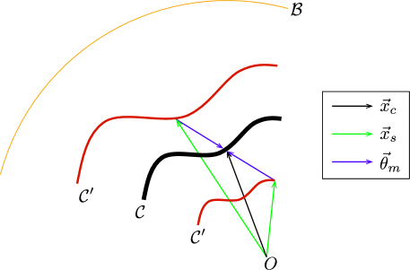
Figure 1: Illustration of Remark 3.6. At the location $\vec{x}_{s}$ such that $\vec{x}_{s}=\vec{x}_{c}$ (black colored vector) and $\vec{\theta}_{m}\cdot\frac{\vec{x}_{c}-\vec{x}_{s}}{|\vec{x}_{c}-\vec{x}_{s}|}=\pm 1$ (green colored vector), true shape of $\mathcal{C}$ and ghost replicas $\mathcal{C}^{\prime}$ will appear, respectively.

4 Numerical experiments

In this section, we exhibit some numerical examples to demonstrate the effectiveness of the proposed algorithm. Throughout this section, the homogeneous domain $\mathcal{D}$ is chosen as the interior region of the two-dimensional unit disk centered at the origin, i.e.,

$$\mathcal{B}=\left\{(\cos t,\sin t):t\in[0,2\pi]\right\}.$$

The adopted wavenumber has the form $k_{f}=\frac{2\pi}{\lambda_{f}}$ for $f=1,2,\cdots,F$; here, $\lambda_{f}$ is the given wavelength that is equi-distributed between $\lambda_{1}=0.7$ and $\lambda_{F}=0.4$. Based on Theorem 3.3, the incident direction $\vec{\theta}_{m}$ is selected as

$$\vec{\theta}_{m}:=\bigg{(}\cos\frac{2(m-1)\pi}{M},\sin\frac{2(m-1)\pi}{M}\bigg{)},\quad m=1,2,\cdots,M,$$

for an even number $M$.

Motivated by [22], we choose two single cracks $\mathcal{C}_{1}$ and $\mathcal{C}_{2}$ as

$$\mathcal{C}_{1} =\left\{\left(0.6t,\frac{1}{2}\cos\frac{t\pi}{2}+\frac{1}{5}\sin\frac{t\pi}{2}-\frac{1}{10}\cos\frac{3t\pi}{2}\right):t\in[-1,1]\right\}$$

$$\mathcal{C}_{2} =\left\{\left(1.5\sin\frac{(3t+4)\pi}{8}-1,0.8\sin\frac{(3t+4)\pi}{4}\right):t\in[-1,1]\right\},$$

and inspired by [34], we choose multiple cracks $\mathcal{C}_{\mathrm{M}}$ as

$$\mathcal{C}_{\mathrm{M}}=\{(t-0.2,-0.5t^{2}+0.5):t\in[-0.5,0.5]\}\cup\{(t+0.2,t^{3}+t^{2}-0.5):s\in[-0.5,0.5]\}.$$

Note that in order to show the robustness of the proposed algorithm, a white Gaussian noise with $15$ dB signal-to-noise ratio (SNR) is added to the unperturbed data.

First, let us consider the imaging result of $\mathcal{C}_{1}$. The left-hand side of Figure 2 shows the map of $\mathbb{R}_{\mathrm{MTD}}(\vec{x}_{s};4)$ for $M=16$ different directions. In this result, because of its small magnitude at $(0.46,0.42)$, $\mathcal{C}_{1}$ appears divided. Moreover, owing to the large magnitude at certain points (for example, $(0.23,0.18)$), we cannot recognize its shape at this stage. The right-hand side of Figure 2 is the map of $\mathbb{R}_{\mathrm{MTD}}(\vec{x}_{s};16)$. The figure shows that there is undivided or whole $\mathcal{C}_{1}$; this means that we obtained a more accurate result than the previous one. However, because certain points have a large magnitude, we cannot determine the true shape of $\mathcal{C}_{1}$.

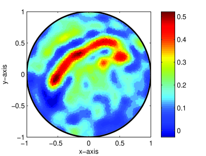
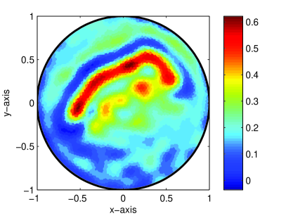
Figure 2: Map of $\mathbb{R}_{\mathrm{MTD}}(\vec{x}_{s};F)$ with $F=16,M=4$ (left) and $F=16,M=16$ (right) for $\mathcal{C}_{1}$.

Figure 3 shows the map of $\mathbb{R}_{\mathrm{MTD}}(\vec{x}_{s};F)$ for crack $\mathcal{C}_{2}$. In contrast with the result of $\mathcal{C}_{1}$, it is difficult to identify the shape of the crack because of the great number of points with large magnitudes. Fortunately, similar to the results in Figure 2, map of $\mathbb{R}_{\mathrm{MTD}}(\vec{x}_{s};16)$ yields a better image than that obtained by the map of $\mathbb{R}_{\mathrm{MTD}}(\vec{x}_{s};4)$.

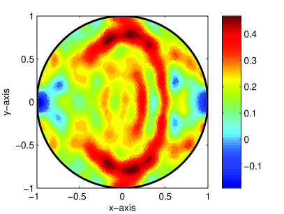
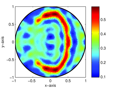
Figure 3: Map of $\mathbb{R}_{\mathrm{MTD}}(\vec{x}_{s};F)$ with $F=16,M=4$ (left) and $F=16,M=16$ (right) for $\mathcal{C}_{2}$.

The application of multiple cracks $\mathcal{C}_{\mathrm{M}}$ is shown in Figure 4. This figure shows the maps of $\mathbb{R}_{\mathrm{TD}}(\vec{x}_{s};\frac{2\pi}{0.4})$ and $\mathbb{R}_{\mathrm{MTD}}(\vec{x}_{s};F)$. Throughout these results, we can observe that the map of $\mathbb{R}_{\mathrm{TD}}(\vec{x}_{s};k)$ yields a poor result even if the number of incident directions $M$ is large; conversely, the multi-frequency imaging function $\mathbb{R}_{\mathrm{MTD}}(\vec{x}_{s};F)$ yields an accurate result even if $M$ is small.

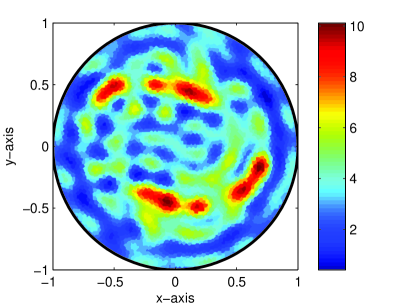
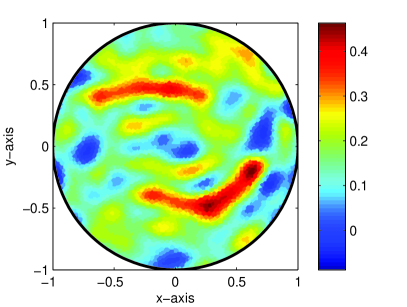
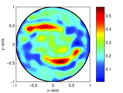
Figure 4: Maps of $\mathbb{R}_{\mathrm{TD}}(\vec{x}_{s};\frac{2\pi}{0.4})$ with $M=32$ (top, left) and $M=64$ (top, right), and maps of $\mathbb{R}_{\mathrm{MTD}}(\vec{x}_{s};F)$ with $F=16,M=4$ (bottom, left) and $F=16,M=16$ (bottom, right) for $\mathcal{C}_{\mathrm{M}}$.

In Figure 5, maps of $\mathbb{R}_{\mathrm{MTD}}(\vec{x}_{s};16)$ with $M=5$ number of incident directions are displayed for cracks $\mathcal{C}_{1}$ and $\mathcal{C}_{\mathrm{M}}$ in order to verify the (P2) of Remark 3.6. By comparing Figures 2 and 4, it is difficult to discern the shape of true crack(s) because of the appearance of unforseen replicas with large magnitudes. Note that if $M$ is an odd number but is sufficiently large enough, the map of $\mathbb{R}_{\mathrm{MTD}}(\vec{x}_{s};F)$ yield a good result, refer to Figure 6.

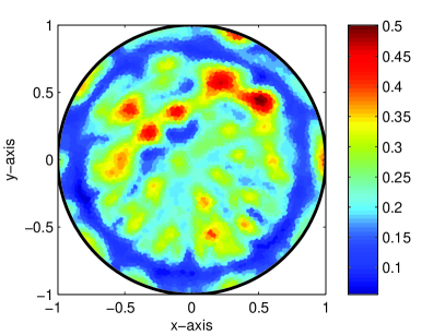
Figure 5: Map of $\mathbb{R}_{\mathrm{MTD}}(\vec{x}_{s};F)$ with $F=16,M=5$ for $\mathcal{C}_{1}$ (left) and $\mathcal{C}_{\mathrm{M}}$ (right).

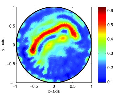
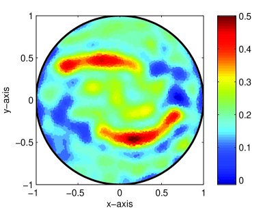
Figure 6: Map of $\mathbb{R}_{\mathrm{MTD}}(\vec{x}_{s};F)$ with $F=16,M=15$ for $\mathcal{C}_{1}$ (left) and $\mathcal{C}_{\mathrm{M}}$ (right).

At this moment, we increase the number of applied frequencies $F$ and incident directions $M$. Figures 7, 8, and 9 depict the map of $\mathbb{R}_{\mathrm{MTD}}(\vec{x}_{s};F)$ when $F=64$ and $M=16$ or $M=64$. As we expected in (P3) of Remark 3.6, the results yielded by $\mathbb{R}_{\mathrm{MTD}}(\vec{x}_{s};F)$ improve with increasing number of $F$ and/or $M$.

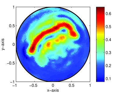
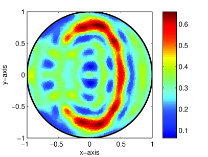
Figure 7: Map of $\mathbb{R}_{\mathrm{MTD}}(\vec{x}_{s};F)$ with $F=16,M=64$ for $\mathcal{C}_{1}$ (left) and $\mathcal{C}_{2}$ (right).

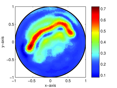
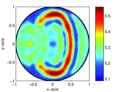
Figure 8: Map of $\mathbb{R}_{\mathrm{MTD}}(\vec{x}_{s};F)$ with $F=64,M=64$ for $\mathcal{C}_{1}$ (left) and $\mathcal{C}_{2}$ (right).

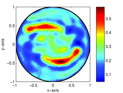
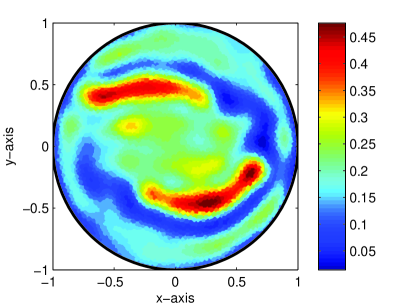
Figure 9: Map of $\mathbb{R}_{\mathrm{MTD}}(\vec{x}_{s};F)$ with $F=16,M=64$ (left) and $F=64,M=64$ (right) for $\mathcal{C}_{\mathrm{M}}$.

Remark 4.7 (Limitation of the multi-frequency topological derivative)

Although multi-frequency topological derivative imaging yields very good imaging results for not only single but also multiple cracks, it still has the following limitations.

1. Let us consider the imaging of a crack of a large curvature near one of the crack tips. To illustrate this, we choose a crack from [23]:

   $$\mathcal{C}_{3}=\left\{(t+t^{2},0.5t^{4}+t):-1\leq t\leq 3\right\}.$$

   From the results in Figure 10, the imaging results yielded by $\mathbb{R}_{\mathrm{MTD}}(\vec{x}_{s};F)$ are satisfactory. However, at the point of the large curvature, the map of $\mathbb{R}_{\mathrm{MTD}}(\vec{x}_{s};F)$ reconstructs a slightly different shape of the crack.

2. We apply the proposed algorithm for imaging an oscillation crack represented as follows:

   $$\mathcal{C}_{4}=\left\{(t,0.5t^{2}+0.1\sin(3\pi(t+0.7))):-0.6\leq t\leq 0.6\right\}.$$

   Figure 11 shows the map of $\mathbb{R}_{\mathrm{MTD}}(\vec{x}_{s};F)$. The obtained result by the proposed algorithm does not improve even when the number of $F$ and $M$ are increased. The proposed algorithm requires further optiization.

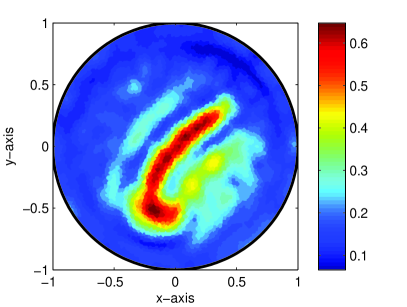
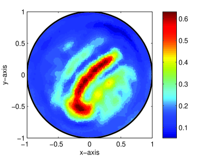
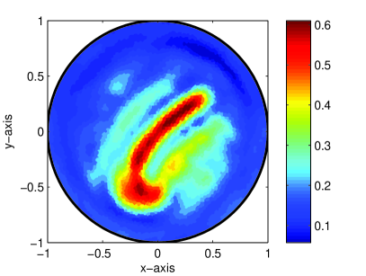
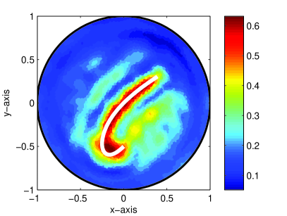
Figure 10: Map of $\mathbb{R}_{\mathrm{MTD}}(\vec{x}_{s};F)$ for $\mathcal{C}_{3}$ with $F=16,M=16$ (top, left), $F=16,M=64$ (top, right), $F=64,M=64$ (bottom, left) and true shape (bottom, right).

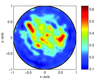
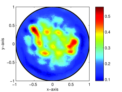
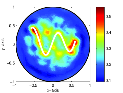
Figure 11: Same as Figure 10 except the crack is $\mathcal{C}_{4}$.

5 Concluding remarks

We improved the traditional topological derivative concept to determine location and reconstruct the shape of arbitrary-shaped curve-like perfectly conducting cracks. For this purpose, we designed a reconstruction algorithm based on the multi-frequency topological derivative, analyzed its structure, and investigated its properties. We confirmed that the multi-frequency topological derivative contains singularity on the cracks, and therefore it reaches its maximum value at the location of the cracks. Moreover, we demonstrated that why ghost replicas appeared in the neighborhood of cracks and why the configuration of symmetric incident directions yields better results than the non-symmetric configuration. Numerical simulations under various situations depicted both the benefits and limitations of the proposed algorithm. Because the algorithm requires only a one-step iteration procedure, it is very fast in terms of shape identification but does not yield the complete shape of cracks. However, by adopting the obtained result as a starting point of a Newton-type based algorithm [22], it is expected that complete shape reconstruction can be successfully accomplished.

This paper deals with the reconstruction of perfectly conducting cracks with Dirichlet boundary condition. Accordingly, the extension of this research to the crack with Neumann boundary condition will be an interesting work. We believe that applying higher-order terms in the asymptotic expansion formula [9] give a higher order topological derivative [13]. The calculation and analysis of higher-order topological derivative will be a valuable research topic. According to the Statistical Hypothesis Testing [6], multi-frequencies are expected to enhance the imaging performance. The corresponding work will include a careful stability and resolution analysis of the multi-frequency topological derivative.

References

[1]M. Abramowitz and I. A. Stegun, Handbook of Mathematical Functions, with Formulas, Graphs, and Mathematical Tables, (1996), Dover, New York.
[2]D. Álvarez, O. Dorn, N. Irishina, and M. Moscoso, Crack reconstruction using a level-set strategy, J. Comput. Phys., 228 (2009), 5710–5721.
[3]H. Ammari, An Introduction to Mathematics of Emerging Biomedical Imaging, Mathematics and Applications Series, 62 (2008), Springer-Verlag, Berlin.
[4]H. Ammari, Mathematical Modeling in Biomedical Imaging II: Optical, Ultrasound, and Opto-Acoustic Tomographies, Lecture Notes in Mathematics, 2035 (2011), Springer-Verlag, Berlin.
[5]H. Ammari, J. Garnier, V. Jugnon, and H. Kang, Stability and resolution analysis for a topological derivative based imaging functional, SIAM J. Control. Optim., 50 (2012), 48–76.
[6]H. Ammari, J. Garnier, H. Kang, W.-K. Park, and K. Sølna, Imaging schemes for perfectly conducting cracks, SIAM J. Appl. Math., 71 (2011), 68–91.
[7]H. Ammari, E. Iakovleva and D. Lesselier, A MUSIC algorithm for locating small inclusions buried in a half-space from the scattering amplitude at a fixed frequency, Multiscale Model. Simul. 3 (2005), 597–628.
[8]H. Ammari, E. Iakovleva and D. Lesselier, Two numerical methods for recovering small electromagnetic inclusions from the scattering amplitude at a fixed frequency, SIAM J. Sci. Comput., 27 (2005), 130–158.
[9]H. Ammari and H. Kang, Reconstruction of Small Inhomogeneities from Boundary Measurements, Lecture Notes in Mathematics, 1846 (2004), Springer-Verlag, Berlin.
[10]H. Ammari, H. Kang, H. Lee and W.-K. Park, Asymptotic imaging of perfectly conducting cracks, SIAM J. Sci. Comput., 32 (2010), 894–922.
[11]H. Ammari, S. Moskow and M. S. Vogelius, Boundary integral formulae for the reconstruction of electric and electromagnetic inhomogeneities of small volume, 9 (2003), 49–66.
[12]D. Auroux and M. Masmoudi, Image processing by topological asymptotic analysis, ESAIM Proc., 26 (2009), 24–44.
[13]M. Bonnet, Fast identification of cracks using higher-order topological sensitivity for 2-D potential problems, Eng. Anal. Bound. Elem., 35 (2011), 223–235.
[14]A. Carpio and M.-L. Rapun, Solving inhomogeneous inverse problems by topological derivative methods, Inverse Probl., 24 (2008), 045014.
[15]M. Cheney, The linear sampling method and the MUSIC algorithm, Inverse Probl., 17 (2001), 591–595.
[16]M. Donelli, A rescue radar system for the detection of victims trapped under rubble based on the independent component analysis algorithm, Prog. Electromagn. Res. M, 19 (2011), 173–181.
[17]R. Douvenot, M. Lambert and D. Lesselier, Adaptive metamodels for crack characterization in eddy-current testing, IEEE Trans. Magn., 47 (2011), 746–755.
[18]O. Dorn and D. Lesselier, Level set methods for inverse scattering, Inverse Probl. 22 (2006), R67–R131.
[20]Y. D. Jo, Y. M. Kwon, J. Y. Huh and W.-K. Park, Structure analysis of single- and multi-frequency imaging functions in inverse scattering problems, submitted, available at http://arxiv.org/abs/1208.0641.
[21]A. Kirsch and S. Ritter, A linear sampling method for inverse scattering from an open arc, Inverse Probl. 16 (2000), 89–105.
[22]R. Kress, Inverse scattering from an open arc, Math. Methods Appl. Sci., 18 (2003), 267–293.
[23]R. Kress and P. Serranho, A hybrid method for two-dimensional crack reconstruction, Inverse Probl., 21 (2005), 773–784.
[24]Y.-K. Ma, P.-S. Kim and W.-K. Park, Analysis of topological derivative function for a fast electromagnetic imaging of perfectly conducing cracks, Prog. Electromagn. Res., 122 (2012), 311–325.
[25]N. Nemitz and M. Bonnet, Topological sensitivity and FMM-accelerated BEM applied to 3D acoustic inverse scattering, Eng. Anal. Bound. Elem., 32 (2008), 957–970.
[27]W.-K. Park, Multi-frequency topological derivative for approximate shape acquisition of curve-like thin electromagnetic inhomogeneities, available at http://arxiv.org/abs/1207.0582.
[28]W.-K. Park, Non-iterative imaging of thin electromagnetic inclusions from multi-frequency response matrix, Prog. Electromagn. Res., 106 (2010), 225–241.
[29]W.-K. Park, On the imaging of thin dielectric inclusions buried within a half-space, Inverse Probl., 26 (2010), 074008.
[30]W.-K. Park, On the imaging of thin dielectric inclusions via topological derivative concept, Prog. Electromagn. Res., 110 (2010), 237–252.
[31]W.-K. Park, Topological derivative strategy for one-step iteration imaging of arbitrary shaped thin, curve-like electromagnetic inclusions, J. Comput. Phys., 231 (2012), 1426–1439.
[32]W.-K. Park and D. Lesselier, Electromagnetic MUSIC-type imaging of perfectly conducting, arc-like cracks at single frequency, J. Comput. Phys., 228 (2012), 8093–8111.
[33]W.-K. Park and D. Lesselier, Fast electromagnetic imaging of thin inclusions in half-space affected by random scatterers, Waves Random Complex Media, 22 (2012), 3–23.
[34]W.-K. Park and D. Lesselier, MUSIC-type imaging of a thin penetrable inclusion from its far-field multi-static response matrix, Inverse Probl., 25 (2009), 075002.
[35]W.-K. Park and D. Lesselier, Reconstruction of thin electromagnetic inclusions by a level set method, Inverse Probl., 25 (2009), 085010.
[37]B. Scholz, Towards virtual electrical breast biopsy: space frequency MUSIC for trans-admittance data, IEEE. Trans. Med. Imaging, 21 (2002), 588–595.
[38]J. Sokołowski and A. Zochowski, On the topological derivative in shape optimization, SIAM J. Control Optim., 37 (1999), 1251–1272.