Robust Dequantized Compressive Sensing

Abstract

We consider the reconstruction problem in compressed sensing in which the observations are recorded in a finite number of bits. They may thus contain quantization errors (from being rounded to the nearest representable value) and saturation errors (from being outside the range of representable values). Our formulation has an objective of weighted $\ell_{2}$-$\ell_{1}$ type, along with constraints that account explicitly for quantization and saturation errors, and is solved with an augmented Lagrangian method. We prove a consistency result for the recovered solution, stronger than those that have appeared to date in the literature, showing in particular that asymptotic consistency can be obtained without oversampling. We present extensive computational comparisons with formulations proposed previously, and variants thereof.

1 Introduction

This paper considers a compressive sensing (CS) system in which the measurements are represented by a finite number of bits, which we denote by $B$. By defining a quantization interval $\Delta>0$, and setting $G:=2^{B-1}\Delta$, we obtain the following values for representable measurements:

$$-G+\frac{\Delta}{2},-G+\frac{3\Delta}{2},\dotsc,-\frac{\Delta}{2},\frac{\Delta}{2},\dotsc,G-\frac{\Delta}{2}.$$ (1)

We assume in our model that actual measurements are recorded by rounding to the nearest value in this set. The recorded observations thus contain (a) quantization errors, resulting from rounding of the true observation to the nearest represented number, and (b) saturation errors, when the true observation lies beyond the range of represented values, namely, $[-G+\frac{\Delta}{2},G-\frac{\Delta}{2}]$. This setup is seen in some compressive sensing hardware architectures [see, for example, 15, 20, 19, 21, 9].

Given a sensing matrix $\Phi\in\mathbb{R}^{M\times N}$ and the unknown vector $x$, the true observations (without noise) would be $\Phi x$. We denote the recorded observations by the vector $y\in\mathbb{R}^{M}$, whose components take on the values in (1). We partition $\Phi$ into the following three submatrices:

• The saturation parts $\bar{\Phi}_{-}$ and $\bar{\Phi}_{+}$, which correspond to those recorded measurements that are represented by $-G+{\Delta/2}$ or $G-{\Delta/2}$, respectively — the two extreme values in (1). We denote the number of rows in these two matrices combined by $\bar{M}$.

• The unsaturated part $\tilde{\Phi}\in\mathbb{R}^{\tilde{M}\times N}$, which corresponds to the measurements that are rounded to non-extreme representable values.

In some existing analyses [5, 13], the quantization errors are treated as a random variables following an i.i.d. uniform distribution in the range $[-{\Delta\over 2},{\Delta\over 2}]$. This assumption makes sense in many situations (for example, image processing, audio/video processing), particularly when the quantization interval $\Delta$ is tiny. However, the assumption of a uniform distribution may not be appropriate when $\Delta$ is large, or when an inappropriate choice of saturation level $G$ is made. In this paper, we assume a slightly weaker condition, namely, that the quantization errors for non-saturated measurements are independent random variables with zero expectation. (These random variables are of course bounded uniformly by $\Delta/2$.)

The state-of-the-art formulation to this problem [see 14] is to combine the basis pursuit model with saturation constraints, as follows:

$$\min_{x}~{} \|x\|_{1}$$ (2a)

$$\mbox{s.t.}\quad\|\tilde{\Phi}x-\tilde{y}\|^{2} \leq\epsilon^{2}\Delta^{2}\; \ell_{2}$$ () (2b)

$$\bar{\Phi}_{+}x \geq(G-\Delta)\mathbb{1}\; +$$ ( saturation) (2c)

$$\bar{\Phi}_{-}x \leq(\Delta-G)\mathbb{1},\; -$$ ( saturation) (2d)

where $\mathbb{1}$ is a column vector with all entries equal to $1$ and $\tilde{y}$ is the quantized subvector of the observation vector $y$ that corresponds to the unsaturated measurements. We refer to this model as “L2 ” in later discussions. It has been shown that the estimation error arising from the formulation (2) is bounded by $O(\epsilon\Delta)$ in the $\ell_{2}$ norm sense [see 14, 6, 13].

The paper proposes a robust model that replaces (2b) with a least-square loss term in the objective and adds an $\ell_{\infty}$ constraint:

$$\min_{x}~{}{1\over 2}\|\tilde{\Phi}x-\tilde{y}\|^{2} +\lambda\Delta\|x\|_{1}$$ (3a)

$$\mbox{s.t.}\quad\|\tilde{\Phi}x-\tilde{y}\|_{\infty} \leq\Delta/2\; \ell_{\infty}$$ () (3b)

$$\bar{\Phi}_{+}x \geq(G-\Delta)\mathbb{1}\; +$$ ( saturation) (3c)

$$\bar{\Phi}_{-}x \leq(\Delta-G)\mathbb{1}.\; -$$ ( saturation) (3d)

We refer to this model as LASSO$\infty$ in later discussions. The $\ell_{\infty}$ constraint (3b) arises from the fact that (unsaturated) quantization errors are bounded by $\Delta/2$. This constraint may reduce the feasible region for the recovery problem while retaining feasibility of the true solution $x^{*}$, thus promoting more robust signal recovery. From the viewpoint of optimization, the constraint (2b) plays the same role as the least-square loss term in the objective (3a), when the values of $\epsilon$ and $\lambda$ are related appropriately. However, it will become clear from our analysis that inclusion of this term in the objective rather than applying the constraint (2b) can lead a tighter bound on the reconstruction error.

The analysis in this paper shows that when $\Phi$ is a Gaussian ensemble, and provided that $S\log N=o(M)$ and several mild conditions hold, the estimation error of for the solution of (3) is bounded by

$$\min\left\{O\left(\sqrt{S(\log N)/M}\right),O(1)\right\}\Delta,$$

with high probability, where $S$ is the sparsity (the number of nonzero components in $x^{*}$). This estimate implies that solutions of (3) are, in the worst case, better than the state-of-the-art model (2), and also better than the model in which only the $\ell_{\infty}$ constraint (3b) are applied (in place of the $\ell_{2}$ constraint (2b)), as mentioned by [13]. More importantly, when the number $\tilde{M}$ of unsaturated measurements goes to infinity faster than $S\log(N)$, the estimation error for the solution of (3) vanishes with high probability. (The model (2) does not indicate such an improvement when more measurements are available.) Although Jacques et al. [13] show that the estimation error can be eliminated only using an $\ell_{p}$ constraint (in place of the $\ell_{2}$ constraint (2b)) when $p\rightarrow\infty$, the oversampling condition (that is, the number of observations required) is more demanding than for our formulation (3).

We use the alternating direction method of multipliers (ADMM) [see 10, 4] to solve (3). The computational results reported in Section 4 compare the solution properties for (3) to those for (2) and other formulations. In some of our examples, we consider choices for the parameter $\lambda$ and $\epsilon$ that admit the true solution $x^{*}$ as a feasible point with a specified level of confidence. We find that for these choices of $\lambda$ and $\epsilon$, the model (3) yields more accurate solutions than the alternatives, where the signal is sparse and high confidence is desired.

1.1 Related Work

There have been several recent works on CS with quantization and saturation. Laska et al. [14] propose the formulation (2). Jacques et al. [13] replace the $\ell_{2}$ constraint (2b) by an $\ell_{p}$ constraint ($2\leq p<\infty$) to handle the oversampling case, and show that values $p$ greater than $2$ lead to an improvement of factor $1/\sqrt{p+1}$ on the bound of error in the recovered signal. The model of Zymnis et al. [25] allows Gaussian noise in the measurements before quantization, and solves the resulting formulation with an $\ell_{1}$-regularized maximum likelihood formulation. The average distortion introduced by scalar, vector, and entropy coded quantization of CS is studied by Dai et al. [8].

The extreme case of 1-bit CS (in which only the sign of the observation is recorded) has been studied by Gupta et al. [11] and Boufounos and Baraniuk [3]. In the latter paper, the $\ell_{1}$ norm objective is minimized on the unit ball, with a sign consistency constraint. The former paper proposes two algorithms that require at most $O(S\log N)$ measurements to recover the unknown support of the true signal (though they cannot recover the magnitudes of the nonzeros reliably).

1.2 Notation

We use $\|\cdot\|_{p}$ to denote the $\ell_{p}$ norm, where $1\leq p\leq\infty$, with $\|\cdot\|$ denoting the $\ell_{2}$ norm. We use $x^{*}$ for the true signal, $\hat{x}$ as the estimated signal (the solution of (3)), and $h=\hat{x}-x^{*}$ as the difference. As mentioned above, $S$ denotes the number of nonzero elements of $x^{*}$.

For any $z\in\mathbb{R}^{N}$, we use $z_{i}$ to denote the $i$th component and $z_{T}$ to denote the subvector corresponding to index set $T\subset\{1,2,...,N\}$. Similarly, we use $\tilde{\Phi}_{T}$ to denote the column submatrix of $\tilde{\Phi}$ consisting of the columns indexed by $T$. The cardinality of $T$ is denoted by $|T|$. We use $\tilde{\Phi}_{i}$ to denote the $i$th column of $\tilde{\Phi}$.

In discussing the dimensions of the problem and how they are related to each other in the limit (as $N$ and $\tilde{M}$ both approach $\infty$), we make use of order notation. If $\alpha$ and $\beta$ are both positive quantities that depend on the dimensions, we write $\alpha=O(\beta)$ if $\alpha$ can be bounded by a fixed multiple of $\beta$ for all sufficiently large dimensions. We write $\alpha=o(\beta)$ if for any positive constant $\phi>0$, we have $\alpha\leq\phi\beta$ for all sufficiently large dimensions. We write $\alpha=\Omega(\beta)$ if both $\alpha=O(\beta)$ and $\beta=O(\alpha)$.

The projection onto the $\ell_{\infty}$ norm ball with the radius $\lambda$ is

$$\mathcal{P}_{\infty}(x,\lambda):=\mbox{sign}(x)\odot\min(|x|,\lambda)$$

where $\odot$ denotes componentwise multiplication and $\mbox{sign}(x)$ is the sign vector of $x$. (The $i$th entry of $\mbox{sign}(x)$ is $1$, $-1$, or $0$ depending on whether $x_{i}$ is positive, negative, or zero, respectively.)

The indicator function $\mathbb{I}_{\Pi}(\cdot)$ for a set $\Pi$ is defined to be $0$ on $\Pi$ and $\infty$ otherwise.

We partition the sensing matrix $\Phi$ according to saturated and unsaturated measurements as follows:

$$\bar{\Phi}=\left[\begin{matrix}-\bar{\Phi}_{-}\\ \bar{\Phi}_{+}\end{matrix}\right]~{}\text{and}~{}\Phi=\left[\begin{matrix}\tilde{\Phi}\\ \bar{\Phi}\end{matrix}\right].$$ (4)

The maximum column norm in $\tilde{\Phi}$ is denoted by $f_{\max}$, that is,

$$f_{\max}:=\max_{i\in\{1,2,\dotsc,N\}}\|\tilde{\Phi}_{i}\|.$$ (5)

We define the following quantities associated with a matrix $\Psi$ with $N$ columns:

$$\rho^{-}(k,\Psi) :=\min_{|T|\leq k,h\in\mathbb{R}^{N}}{\|\Psi_{T}h_{T}\|^{2}\over\|h_{T}\|^{2}}$$ (6a)

$$\rho^{+}(k,\Psi) :=\max_{|T|\leq k,h\in\mathbb{R}^{N}}{\|\Psi_{T}h_{T}\|^{2}\over\|h_{T}\|^{2}}.$$ (6b)

We use the following abbrevations in some places:

$$\rho^{-}(k):=\rho^{-}(k,\Phi),\quad {\rho}^{+}(k):={\rho}^{+}(k,\Phi),$$

$$\tilde{\rho}^{-}(k):={\rho}^{-}(k,\tilde{\Phi}),\quad \tilde{\rho}^{+}(k):={\rho}^{+}(k,\tilde{\Phi}),$$

$$\bar{\rho}^{-}(k):={\rho}^{-}(k,\bar{\Phi}),\quad \bar{\rho}^{+}(k):={\rho}^{+}(k,\bar{\Phi}).$$

Finally, we denote $(z)+:=\max\{z,0\}$.

1.3 Organization

The ADMM optimization framework for solving (3) is discussed in Section 2. Section 3 analyzes the properties of the solution of (3) in the worst case and compares with existing results. Numerical simulations and comparisons of various formulations are reported in Section 4 and some conclusions are offered in Section 5. Proofs of the claims in Section 3 appear in the appendix.

2 Algorithm

This section describes the ADMM algorithm for solving (3). For simpler notation, we combine the saturation constraints as follows:

$$\left[\begin{matrix}-\bar{\Phi}_{-}\\ \bar{\Phi}_{+}\end{matrix}\right]x\geq\left[\begin{matrix}(G-\Delta)\mathbb{1}\\ (G-\Delta)\mathbb{1}\end{matrix}\right]\;\;\Leftrightarrow\;\;\bar{\Phi}x\geq\bar{y},$$

where $\bar{\Phi}$ is defined in (4) and $\bar{y}$ is defined in an obvious way. To specify ADMM, we introduce auxiliary variables $u$ and $v$, and write (3) as follows.

$$\min_{x}{} {1\over 2}\|\tilde{\Phi}x-\tilde{y}\|^{2}+\lambda\|x\|_{1}$$ (7)

$$\mbox{s.t.}\quad u =\tilde{\Phi}x-\tilde{y}$$

$$v =\bar{\Phi}x-\bar{y}$$

$$\|u\|_{\infty} \leq\Delta/2$$

$$v \geq\mathbb{0}.$$

Introducing Lagrange multipliers $\alpha$ and $\beta$ for the two equality constraints in (7), we write the augmented Lagrangian for this formulation, with prox parameter $\theta>0$ as follows:

$$L_{A}(x,u,v,\alpha,\beta) ={1\over 2}\|\tilde{\Phi}x-\tilde{y}\|^{2}+\lambda\|x\|_{1}+\langle\alpha,u-\tilde{\Phi}x+\tilde{y}\rangle+\langle\beta,v-\bar{\Phi}x+\bar{y}\rangle$$

$$\quad+{\theta\over 2}\|u-\tilde{\Phi}x+\tilde{y}\|^{2}+{\theta\over 2}\|v-\bar{\Phi}x+\bar{y}\|^{2}+\mathbb{I}_{\|u\|_{\infty}\leq\Delta/2}(u)+\mathbb{I}_{v\geq 0}(v)$$

At each iteration of ADMM, we optimize this function with respect to the primal variables $u$ and $v$ in turn, then update the dual variables $\alpha$ and $\beta$ in a manner similar to gradient descent. The penalty parameter $\theta$ may be increased before proceeding to the next iteration.

We summarize the ADMM algorithm in Algorithm 1.

Algorithm 1 ADMM for (7)

0:  $\tilde{\Phi}$, $\tilde{y}$, $\bar{\Phi}$, $\bar{y}$, $\Delta$, $K$, and $x$;

1:  Initialize $\theta>0$, $\alpha=0$, $\beta=0$, $u=\tilde{\Phi}x-\tilde{y}$, and $v=\bar{\Phi}x-\bar{y}$;

2:  for $k=0:K$ do

3:     $u\leftarrow\arg\min_{u}\,L_{A}(x,u,v,\alpha,\beta)$, that is, $u\leftarrow\mathcal{P}_{\infty}(\tilde{\Phi}x-\tilde{y}-\alpha/\theta,\Delta/2)$;

4:     $v\leftarrow\arg\min_{v}\,L_{A}(x,u,v,\alpha,\beta)$, that is, $v\leftarrow\max(\bar{\Phi}x-\bar{y}-\beta/\theta,0)$;

5:      $x\leftarrow\arg\min_{x}\,L_{A}(x,u,v,\alpha,\beta)$;

6:     $\alpha\leftarrow\alpha+\theta(u-\tilde{\Phi}x+\tilde{y})$;

7:     $\beta\leftarrow\beta+\theta(v-\bar{\Phi}x+\bar{y})$;

8:     Possibly increase $\theta$;

9:     if stopping criteria is satisfied then

10:        break;

11:     end if

12:  end for

The updates in Steps 3 and 4 have closed-form solutions, as shown. The function to be minimized in Step 5 consists of an $\|x\|_{1}$ term in conjunction with a quadratic term in $x$. Many algorithms can be applied to solve this problem, e.g., the SpaRSA algorithm [23], the accelerated first order method [18], and the FISTA algorithm [1]. The update strategy for $\theta$ in Step 7 is flexible. We use the following simple and useful scheme from He et al. [12] and Boyd et al. [4]:

$$\theta:=\left\{\begin{aligned} &\theta\tau&&\text{if $\|r\|>\mu\|d\|$}\\ &\theta/\tau&&\text{if $\|r\|<\mu\|d\|$}\\ &\theta&&\text{otherwise},\end{aligned}\right.$$ (8)

where $r$ and $d$ denote the primal and dual residual errors respectively, specifically,

$$r=\left[\begin{matrix}u-\tilde{\Phi}x+\tilde{y}\\ v-\bar{\Phi}v+\bar{y}\end{matrix}\right]~{}\text{and}~{}d=\theta\left[\begin{matrix}\tilde{\Phi}(x-x_{\mbox{\rm\scriptsize last}})\\ \bar{\Phi}(x-x_{\mbox{\rm\scriptsize last}})\end{matrix}\right],$$

where $x_{\mbox{\rm\scriptsize last}}$ denotes the previous value of $x$. The parameters $\mu$ and $\tau$ should be greater than $1$; we used $\mu=10$ and $\tau=2$. Convergence results for ADMM can be found in [4], for example.

3 Analysis

The section analyzes the properties of the solution obtained from our formulation (3). In Subsection 3.1, we obtain bounds on the norm of the difference $h$ between the estimator $\hat{x}$ given by (3) and the true signal $x^{*}$. Our bounds require the true solution $x^{*}$ to be feasible for the formulation (3); we derive conditions that guarantee that this condition holds, with a specified probability. In Subsection 3.2, we estimate the constants that appear in our bounds under certain assumptions, including an assumption that the full sensing matrix $\Phi$ is Gaussian.

We formalize our assumption about quantization errors as follows.

Assumption 1.

The quantization errors $(\tilde{\Phi}x^{*}-\tilde{y})_{i}$, $i=1,2,\dotsc,\tilde{M}$ are independently distributed with expectation $0$.

(Note that since $\tilde{\Phi}$ and $\tilde{y}$ refer to the unsaturated data, the quantization error are bounded uniformly by $\Delta/2$.)

3.1 Estimation Error Bounds

The following error estimate is our main theorem, proved in the appendix.

Theorem 1.

Assume that the true signal $x^{*}$ satisfies

$$\|\tilde{\Phi}^{T}(\tilde{\Phi}x^{*}-\tilde{y})\|_{\infty}\leq\lambda\Delta/2,$$ (9)

for some value of $\lambda$. Let $s$ be a positive integer in the range $1,2,\dotsc,N$, and define

$$\bar{A}_{0}(\Psi):= {\rho}^{-}(2s,\Psi)-3[{\rho}^{+}(3s,\Psi)-{\rho}^{-}(3s,\Psi)]$$ (10a)

$$\bar{A}_{1}(\Psi):= 4[{\rho}^{+}(3s,\Psi)-{\rho}^{-}(3s,\Psi)],$$ (10b)

$$\bar{C}_{1}(\Psi):= 4+{\sqrt{10}A_{1}(\Psi)}/{A_{0}(\Psi)},$$ (10c)

$$\bar{C}_{2}(\Psi):= \sqrt{10/A_{0}(\Psi)}.$$ (10d)

We have that for any $T_{0}\subset\{1,2,...,N\}$ with $s=|T_{0}|$, if $A_{0}(\tilde{\Phi})>0$, then

$$\|h\|\leq 2\bar{C}_{2}(\tilde{\Phi})^{2}\sqrt{s}\lambda\Delta+\left[\bar{C}_{1}(\tilde{\Phi})/\sqrt{s}\right]\|x^{*}_{T_{0}^{c}}\|_{1}+2.5\bar{C}_{2}(\tilde{\Phi})\sqrt{\lambda\Delta\|x^{*}_{T_{0}^{c}}\|_{1}},$$ (11a)

$$\|h\|\leq \bar{C}_{2}(\tilde{\Phi})\sqrt{\tilde{M}}\Delta+\left[\bar{C}_{1}(\tilde{\Phi})/\sqrt{s}\right]\|x^{*}_{T_{0}^{c}}\|_{1}.$$ (11b)

Suppose that Assumption 1 holds, and let $\pi\in(0,1)$ be given. If we define $\lambda=\sqrt{2\log{2N/\pi}}f_{\max}$ in (3), then with probability at least $P=1-\pi$, the inequalities (11a) and (11b) hold.

From the proof in the appendix, one can see that the estimation error bound  (11a) is mainly determined by the least-squares term in the objective (3a), whereas the estimation error bound (11b) arises from the $L_{\infty}$ constraint (3b).

If we take $T_{0}$ as the support set of $x^{*}$, only the first terms in (11a) and (11b) remain.

The condition $A_{0}(\tilde{\Phi})>0$ is a sort of restricted isometry (RIP) condition required in [14]— it assumes reasonable conditioning of column submatrices of $\tilde{\Phi}$ with $O(S)$ columns. Specifically, the number of measurements $\tilde{M}$ required to satisfy $\bar{A}_{0}(\tilde{\Phi})>0$ and RIP are of the same order: $O(S\log(N))$.

3.2 Estimating the Constants

Here we discuss the effect of the least-squares term and the $\ell_{\infty}$ constraints by comparing the leading terms on the right-hand sides of (11a) and (11b). To simplify the comparison, we make the following assumptions.

• $\Phi$ is a Gaussian random matrix, that is, each entry is i.i.d., drawn from a standard Gaussian distribution $\mathcal{N}(0,1)$.

• the confidence level $P=1-\pi$ is fixed.

• $s$ is equal to the sparsity number $S$.

• $S\log N=o(M)$.

• the saturation ratio $\chi:=\bar{M}/M$ is smaller than a small positive threshold that is defined in Theorem 3.

• $T_{0}$ is taken as the support set of $x^{*}$, so that $x^{*}_{T_{0}^{c}}=0$.

Note that (iii) and (iv) together imply that $s=S\ll M$, while (v) implies that $\tilde{M}=\Omega(M)$.

The discussion following Theorem 3 in Appendix indicates that under these assumptions, the quantities defined in (10c), (10c), and (5) satisfy the following estimates:

$$\bar{C}_{1}(\tilde{\Phi})=\Omega(1),\quad\bar{C}_{2}(\tilde{\Phi})=\Omega(1/\sqrt{M}),\quad f_{\max}=\Omega(\sqrt{M}),$$

with high probability, for sufficiently high dimensions. Using the estimates in Theorem 3, with the setting of $\lambda$ from Theorem 1, we have

$$\bar{C}_{2}(\tilde{\Phi})^{2}\sqrt{s}\lambda\Delta =O\left({\sqrt{S\log N}f_{\max}\Delta\over M}\right)=O\left(\sqrt{S\log N\over M}\Delta\right)\rightarrow 0,$$ (12a)

$$\bar{C}_{2}(\tilde{\Phi})\sqrt{\tilde{M}}\Delta =O\left({\sqrt{\tilde{M}}\Delta\over\sqrt{M}}\right)=O\left(\Delta\right).$$ (12b)

By combining the estimation error bounds (11a) and (11b), we have

$$\|h\|\leq\min\,\left\{O\left(\sqrt{S(\log N)/M}\right),O(1)\right\}\Delta.$$ (13)

In the regime described by assumption (iv), (12a) will be asymptotically smaller than (12b). The bound in (13) has size $O\left(\sqrt{S(\log N)/M}\Delta\right)$, consistent with the upper bound of the Dantzig selector [7] and LASSO [24]. Recall that the estimation error of the formulation (2) is $O\left(\|\tilde{\Phi}x^{*}-\tilde{y}\|/\sqrt{\tilde{M}}\right)$ [13, 14] under the RIP condition, for the number of measurements defined in (iv). Since $\|\tilde{\Phi}x^{*}-\tilde{y}\|=O\left(\sqrt{\tilde{M}}\Delta\right)$ [13], this estimate is consistent with the error that would be obtained if we imposed only the $\ell_{\infty}$ constraint (3b) in our formulation. Note that it does not converge to zero even all assumptions (i)-(vi) hold. Under the assumption (iv), the estimation error for (3) will vanish as the dimensions grow, with probability at least $1-\pi$. By contrast, Jacques et al. [13] do not account for saturation in their formulation and show that the estimation error converges to $0$ using an $\ell_{p}$ constraint in place of (2b) when $p\to\infty$ and oversampling happens — specifically, $M\geq\Omega\left(\left(S\log(N/S)\right)^{p/2}\right)$. Weaker oversampling conditions are available using our formulation (3). For example, ${M}=S(\log N)^{2}$ would produce consistency in our formulation, but not in (2).

4 Simulations

This section compares results for five variant formulations. The first one is our formulation (3), which we refer to as LASSO$\infty$ . We also tried a variant in which the $\ell_{\infty}$ constraint (3b) was omitted from (3). The recovery performance for this variant was uniformly worse than for LASSO$\infty$ , so we do not show it in our figures. (It is, however, sometimes better than the formulations described below, and uniformly better than Dantzig .) The remaining four alternatives are based on the following model, in which the $\ell_{2}$ norm of the residual appears in a constraint (rather than in the objective) and a constraint of Dantzig type also appears:

$$\min_{x}~{} \|x\|_{1}$$ (14a)

$$\mbox{s.t.}\quad\|\tilde{\Phi}x-\tilde{y}\|^{2} \leq\epsilon^{2}\Delta^{2}\; \ell_{2}$$ () (14b)

$$\|\tilde{\Phi}x-\tilde{y}\|_{\infty} \leq\Delta/2\; \ell_{\infty}$$ () (14c)

$$\|\tilde{\Phi}^{T}(\tilde{\Phi}x-\tilde{y})\|_{\infty} \leq\lambda\Delta/2\;$$ (Dantzig) (14d)

$$\bar{\Phi}_{+}x \geq(G-\Delta)\mathbb{1}\; +$$ ( saturation) (14e)

$$\bar{\Phi}_{-}x \leq(\Delta-G)\mathbb{1}.\; -$$ ( saturation) (14f)

The four formulations are obtained from this model as follows.

• L$\infty$ : an $\ell_{\infty}$ constraint model that enforces (14c), (14e), and (14f), but not (14b) or (14d). This model is obtained by letting $p\to\infty$ in Jacques et al. [13] and adding saturation constraints.

• L2 : an $\ell_{2}$ constraint model (that is, the state-of-the-art model (2) [14]) that enforces (14b), (14e), and (14f), but not (14c) or (14d);

• Dantzig : the Dantzig constraint algorithm with saturation constraints, which enforces (14d), (14e), and (14f) but not (14b) or (14c);

• L2Dantzig$\infty$ : the full model defined by (14).

Note that we use the same value of $\lambda$ in (14d) as in (3), since in both cases they lead to a constraint that the true signal $x^{*}$ satisfies $\|\tilde{\Phi}^{T}(\tilde{\Phi}x^{*}-\tilde{y})\|_{\infty}\leq\lambda\Delta/2$ with a certain probability; see (14d) and (9). Readers familiar with the equivalence between LASSO and Dantzig selector [2] may notice that L2Dantzig$\infty$ has similar theoretical error bounds to LASSO$\infty$ . Our computational results show that the practical performance of these two approaches is also similar.

The synthetic data is generated as follows. The measurement matrix $\tilde{\Phi}\in\mathbb{R}^{M\times N}$ is a Gaussian matrix, each entry being independently generated from $\mathcal{N}(0,1/R^{2})$, for a given parameter $R$. The $S$ nonzero elements of $x^{*}$ are in random locations and their values are drawn from independently from $\mathcal{N}(0,1)$. We use $\mbox{SNR}=-20\log_{10}(\|\hat{x}-x^{*}\|/\|x^{*}\|)$ as the error metric, where $\hat{x}$ is the signal recovered from each of the formulations under consideration. Given values of saturation parameter $G$ and number of bits $B$, the interval $\Delta$ is defined accordingly as $\Delta=2^{B-1}G$. All experiments are repeated $30$ times; we report the average performance.

We now describe how the bounds $\lambda$ for (3a) and (14d) and $\epsilon$ for (14b) were chosen for these experiments. Essentially, $\epsilon$ and $\lambda$ should be chosen so that the constraints (14b) and (14d) admit the true signal $x^{*}$ with a a high (specified) probability. There is a tradeoff between tightness of the error estimate and confidence. Larger values of $\epsilon$ and $\lambda$ can give a more confident estimate, since the defined feasible region includes $x^{*}$ with a higher probability, while smaller values provide a tighter estimate. Although Lemma 2 suggests how to choose $\lambda$ and [13] show how to determine $\epsilon$, the analysis it not tight, especially when $M$ and $N$ are not particularly large. We use instead an approach based on simulation and on making the assumption (not used elsewhere in the analysis) that the non-saturated quantization errors $\xi_{i}=(\tilde{\Phi}x^{*}-\tilde{y})_{i}$ are i.i.d. uniform in $U_{[-\Delta/2,\Delta/2]}$. (As noted earlier, this stronger assumption makes sense in some settings, and has been used in previous analyses.) We proceed by generating numerous independent samples of $Z\sim U_{[-\Delta/2,\Delta/2]}$. Given a confidence level $1-\pi$ (for $\pi>0$), we set $\epsilon$ to the value for which $\mathbb{P}(Z\geq\epsilon\Delta)=\pi$ is satisfied empirically. A similar technique is used to determine $\lambda$. When we seek certainty ($\pi=0$, or confidence $P=100\%$), we set $\epsilon$ and $\lambda$ according to the true solution $x^{*}$, that is, $\epsilon=\|\tilde{\Phi}x^{*}-\tilde{y}\|/\Delta$ and $\lambda=2\|\tilde{\Phi}^{T}(\tilde{\Phi}x^{*}-\tilde{y})\|_{\infty}/\Delta$.

To summarize the parameters that are varied in our experiments:

• $M$ and $N$ are dimensions of $\Phi$,

• $S$ is sparsity of solution $x^{*}$,

• $G$ is saturation level,

• $B$ is number of bits,

• $R$ is the inverse standard deviation of the elements of $\Phi$, and

• $P=1-\pi$ denotes the confidence levels, expressed as a percentage.

In Figure 1, we fix the values of $M$, $S$, $G$, $R$, and $P$, choose two values of $B$: 3 and 5. Plots show the average SNRs (over $30$ trials) of the solutions $\hat{x}$ recovered from the five models against the dimension $N$. In this and all subsequent figures, the saturation ratio is defined to be $\bar{M}/M=(M-\tilde{M})/M$, the fraction of extreme measurements. Our LASSO$\infty$ formulation and the full model L2Dantzig$\infty$ give the best recovery performance for small $N$, while for larger $N$, LASSO$\infty$ is roughly tied with the the L2 model. The L$\infty$ and Dantzig models have poorer performance, a pattern that we continue to observe in subsequent tests.

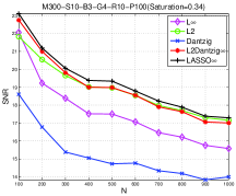
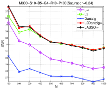
Figure 1: Comparison among various models for fixed values $M=300$, $S=10$, $G=4$, $R=10$, and $P=100\%$, and two values of $B$ (3 and 5, respectively). The graphs show dimension $N$ (horizontal axis) against SNR (vertical axis) for values of $N$ between $100$ and $1000$, averaged over $30$ trials for each combination of parameters.

Figure 2 fixes $N$, $M$, $B$, $G$, $R$, and $P$, and plots SNR as a function of sparsity level $S$. For all models, the quality of reconstruction decreases rapidly with $S$. LASSO$\infty$ and L2Dantzig$\infty$ achieve the best results overall, but are roughly tied with the L2 model for all but the sparsest signals. The L$\infty$ model is competitive for very sparse signals, while the Dantzig model lags in performance.

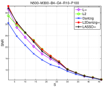
Figure 2: Comparison among various models for $N=500$, $M=300$, $B=4$, $G=0.4$, $R=10$, and $P=100\%$. The graph shows sparsity level $S$ (horizontal axis) plotted against SNR (vertical axis), averaged over $30$ trials.

We now examine the effect of number of measurements $M$ on SNR. Figure 3 fixes $N$, $S$, $G$, $R$, and $P$, and tries two values of $B$: $3$ and $5$, respectively. Figure 4 fixes $B=4$, and allows $N$ to increase with $M$ in the fixed ratio $5/4$. These figures indicate that the LASSO$\infty$ and L2Dantzig$\infty$ models are again roughly tied with the L2 model when the number of measurements is limited. For larger $M$, our models have a slight advantage over the L2 and L$\infty$ models, which is more evident when the quantization intervals are smaller (that is, $B=4$). Another point to note from Figure 4 is that L$\infty$ outperforms L2 when both $M$ and $N$ are much larger than the sparsity $S$.

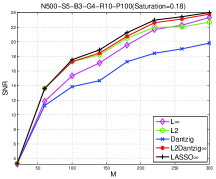
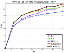
Figure 3: Comparison among various models for fixed values $N=500$, $S=5$, $G=0.4$, $R=15$, and $P=100\%$, and two values of $B$ ($3$ and $5$). The graphs show the number of measurements $M$ (horizontal axis) against SNR (vertical axis) for values of $M$ between $20$ and $300$, averaged over $30$ trials for each combination of parameters.

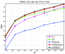
Figure 4: Comparison among various models for fixed ratio $N/M=5/4$, and fixed values $S=10$, $B=4$, $G=0.4$, $R=15$, and $P=100\%$. The graph shows the number of measurements $M$ (horizontal axis) against SNR (vertical axis) for values of $M$ between $100$ and $1680$, averaged over $30$ trials for each combination of parameters.

In Figure 5 we examine the effect of the number of bits $B$ on SNR, for fixed values of $N$, $M$, $S$, $G$, $R$, and $P$. The fidelity of the solution from all models increases linearly with $B$, with the LASSO$\infty$ , L2Dantzig$\infty$ , and L2 models being slightly better than the alternatives.

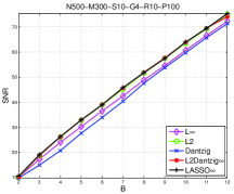
Figure 5: Comparison among various models for fixed values $N=500$, $M=300$, $S=10$, $G=0.4$, $R=10$, and $P=100\%$. This graph shows the bit number $B$ (horizontal axis) against SNR (vertical axis), averaged over $30$ trials.

Next we examine the effect on SNR of the confidence level, for fixed values of $N$, $M$, $B$, $G$, and $R$. In Figure 6, we set $M=300$ and plot results for two values of $S$: 5 and 15. In Figure 7, we use the same values of $S$, but set $M=150$ instead. Note first that the confidence level does not affect the solution of the L$\infty$ model, since this is a deterministic model, so the reconstruction errors are constant for this model. For the other models, we generally see degradation as confidence is higher, since the constraints (14b) and (14d) are looser, so the feasible point that minimizes the objective $\|\cdot\|_{1}$ is further from the optimum $x^{*}$. Again, we see a clear advantage for LASSO$\infty$ when the sparsity is low, $M$ is larger, and the confidence level $P$ is high. For less sparse solutions, the L2 , L2Dantzig$\infty$ , and LASSO$\infty$ models have similar or better performance. In addition, we find that LASSO$\infty$ is more robust to the choice of confidence parameter than other methods (see also Figure 9), although this feature of the method is not evident from our theoretical analysis.

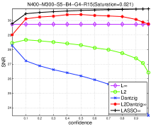
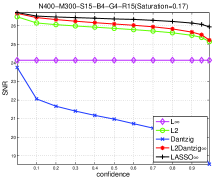
Figure 6: Comparison among various models for fixed values $N=400$, $M=300$, $B=4$, $G=0.4$, and $R=15$, and sparsity levels $S=5$ and $S=15$. The graphs show saturation bound $G$ (horizontal axis) against SNR (vertical axis) for values of $P$ between $0.0001$ and $0.99$, averaged over $30$ trials for each combination of parameters.

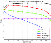
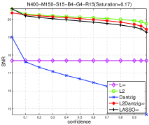
Figure 7: Comparison among various models for fixed values $N=400$, $M=150$, $B=4$, $G=0.4$, and $R=15$, and sparsity levels $S=5$ and $S=15$. The graphs show confidence $P$ (horizontal axis) against SNR (vertical axis) for values of $P$ between $0.0001$ and $0.99$, averaged over $30$ trials for each combination of parameters.

In Figure 8 we examine the effect of saturation bound $G$ on SNR. We fix $N$, $M$, $B$, $R$, and $P$, and try two values of $S$: $5$ and $10$. A tradeoff is evident — the reconstruction performances are not monotonic with $G$. As $G$ increases, the proportion of saturated measurements drops sharply, but the quantization interval also increases, degrading the quality of the measured observations. We again note a slight advantage for the LASSO$\infty$ and L2Dantzig$\infty$ models, with very similar performance by L2 when the oversampling is lower.

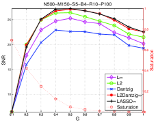
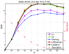
Figure 8: Comparison among various models for fixed values of $N=500$, $M=150$, $B=4$, $R=15$, $P=100\%$, and two values of $S$: $5$ and $10$. The graphs show confidence $P$ (horizontal axis) against SNR (left vertical axis) and saturation ratio (right vertical axis), averaged over $30$ trials for each combination of parameters.

In Figure 9, we fix $N$, $M$, $S$, $B$, $R$, and tune the value of $G$ to achieve specified saturation ratios of $2\%$ and $10\%$. We plot SNR against the confidence level $P$, varied from $0\%$ to $100\%$. Again, we see generally good performance from the LASSO$\infty$ and L2Dantzig$\infty$ models, with L2 being competitive for less sparse solutions.

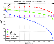
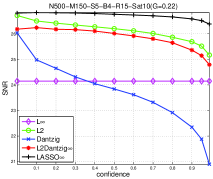
Figure 9: Comparison among various models for fixed values of $N=500$, $M=150$, $S=5$, $B=4$, $R=15$, and two values of saturation ratio: $2\%$ and $10\%$, which are achieved by tuning the value of $G$. The graphs show confidence $P$ (horizontal axis) against SNR (vertical axis), averaged over $30$ trials for each combination of parameters.

Summarizing, we note the following points.

• Our proposed LASSO$\infty$ formulation gives either best or equal-best reconstruction performance in most regimes, with a more marked advantage when the signal is highly sparse and the number of samples is higher.

• The L2 model has similar performance to the full model, and is even slightly better than our model for less sparse signals with fewer measurements, since it is not sensitive to the measurement number as the upper bound suggested by [14]. Although the inequality in (13) also indicates the estimate error by our model is bounded by a constant due to the $\ell_{\infty}$ constraint, the error bound determined by the $\ell_{\infty}$ constraint is not as tight as the $\ell_{2}$ constraint in general. This fact is evident when we compare the the L$\infty$ model with the L2 model.

• The L$\infty$ model performs well (and is competitive with the others) when the number of unsaturated measurements is relatively large.

• The L2Dantzig$\infty$ model is competitive with LASSO$\infty$ if $\epsilon$ and $\lambda$ can be determined from the true signal $x^{*}$. Otherwise, LASSO$\infty$ is more robust to choices of these parameters that do not require knowledge of the true signals, especially if a high confidence level is desired.

5 Conclusion

We have analyzed a formulation of the reconstruction problem from compressed sensing in which the measurements are quantized to a finite number of possible values. Our formulation uses an objective of $\ell_{2}$-$\ell_{1}$ type, along with explicit constraints that restrict the individual quantization errors to known intervals. We obtain bounds on the estimation error, and estimate these bounds for the case in which the sensing matrix is Gaussian. Finally, we prove the practical utility of our formulation by comparing with an approach that has been proposed previously, along with some variations on this approach that attempt to distil the relative importance of different constraints in the formulation.

Appendix A

This section contains the proof to a more general form of Theorem 1, developed via a number of technical lemmas. At the end, we state and prove a result (Theorem 3) concerning high-probability estimates of the bounds under additional assumptions on the sensing matrix $\tilde{\Phi}$.

Theorem 1 is a corollary of the following more general result.

Theorem 2.

Assume that the true signal $x^{*}$ satisfies

$$\|\tilde{\Phi}^{T}(\tilde{\Phi}x^{*}-\tilde{y})\|_{\infty}\leq\lambda\Delta/2,$$ (15)

for some value of $\lambda$. Let $s$ and $l$ be positive integers in the range $1,2,\dotsc,N$, and define

$$A_{0}(\Psi):= {\rho}^{-}(s+l,\Psi)-3{\sqrt{s/l}}\left[{\rho}^{+}(s+2l,\Psi)-{\rho}^{-}(s+2l,\Psi)\right]$$ (16a)

$$A_{1}(\Psi):= 4[{\rho}^{+}(s+2l,\Psi)-{\rho}^{-}(s+2l,\Psi)],$$ (16b)

$$C_{1}(\Psi):= 4+{\sqrt{(1+9s/l)}A_{1}(\Psi)}/{A_{0}(\Psi)},$$ (16c)

$$C_{2}(\Psi):= \sqrt{(1+9s/l)/A_{0}(\Psi)}.$$ (16d)

We have that for any $T_{0}\subset\{1,2,...,N\}$ with $s=|T_{0}|$, if $A_{0}(\tilde{\Phi})>0$, then

$$\|h\|\leq \frac{6C_{2}(\tilde{\Phi})^{2}\sqrt{s}\lambda\Delta}{\sqrt{1+9s/l}}+\frac{C_{1}(\tilde{\Phi})}{\sqrt{l}}\|x^{*}_{T_{0}^{c}}\|_{1}+2.5{C_{2}(\tilde{\Phi})}\sqrt{\lambda\Delta\|x_{T_{0}^{c}}^{*}\|_{1}},$$ (17a)

$$\|h\|\leq C_{2}(\tilde{\Phi})\sqrt{\tilde{M}}\Delta+\frac{C_{1}(\tilde{\Phi})}{\sqrt{l}}\|x^{*}_{T_{0}^{c}}\|_{1}.$$ (17b)

Suppose that Assumption 1 holds, and let $\pi\in(0,1)$ be given. If we define $\lambda=\sqrt{2\log{2N/\pi}}f_{\max}$ in (3), then with probability at least $P=1-\pi$, the inequalities (17a) and (17b) hold.

Theorem 1 can be proven by setting $s=l$ in Theorem 2 and defining $\bar{C}_{1}(\tilde{\Phi})$ to be $C_{1}(\Psi)$ for $l=s$ and $\Psi=\tilde{\Phi}$, and similarly for $\bar{C}_{1}(\tilde{\Phi})$, $\bar{A}_{0}(\tilde{\Phi})$, and $\bar{A}_{1}(\tilde{\Phi})$.

The proof of Theorem 2 essentially follows the standard analysis procedure in compressive sensing. Some similar lemmas and proofs can be found in Bickel et al. [2], Candès and Tao [7], Candès [6], Zhang [24], Liu et al. [16, 17]. For completeness, we include all proofs in the following discussion.

Given the error vector $h=\hat{x}-x^{*}$ and the set $T_{0}$ (with $s$ entries), divide the complementary index set $T_{0}^{c}:=\{1,2,...,N\}\backslash T_{0}$ into a group of subsets $T_{j}$’s ($j=1,2,\dotsc,J$), without intersection, such that $T_{1}$ indicates the index set of the largest $l$ entries of $h_{T_{0}^{c}}$, $T_{2}$ contains the next-largest $l$ entries of $h_{T_{0}^{c}}$, and so forth.

Lemma 1.

We have

$$\|\tilde{\Phi}h\|_{\infty} \leq\Delta.$$ (18)

Proof.

From (3b), and invoking feasibility of $\hat{x}$ and $x^{*}$, we obtain

$$\|\tilde{\Phi}h\|_{\infty}=\|\tilde{\Phi}(\hat{x}-x^{*})\|_{\infty}\leq\|\tilde{\Phi}\hat{x}-\tilde{y}\|_{\infty}+\|\tilde{\Phi}x^{*}-\tilde{y}\|_{\infty}\leq\Delta.$$

∎

Lemma 2.

Suppose that Assumption 1 holds. Given $\pi\in(0,1)$, the choice $\lambda=\sqrt{2\log{(2N/\pi)}}f_{\max}$ ensures that the true signal $x^{*}$ satisfies (15), that is

$$\|\tilde{\Phi}^{T}(\tilde{\Phi}x^{*}-\tilde{y})\|_{\infty}\leq\lambda\Delta/2$$

with probability at least $1-\pi$.

Proof.

Define the random variable $Z_{j}=\tilde{\Phi}_{j}^{T}(\tilde{\Phi}x^{*}-\tilde{y})=\tilde{\Phi}_{j}^{T}\xi$, where $\xi=[\xi_{1},...,\xi_{\tilde{M}}]$ is defined in an obvious way. (Note that $\|Z\|_{\infty}=\|\tilde{\Phi}^{T}(\tilde{\Phi}x^{*}-\tilde{y})\|_{\infty}$.) Since $\mathbb{E}(Z_{j})=0$ (from Assumption 1) and all $\tilde{\Phi}_{ij}\xi_{i}$’s are in the range $[-\tilde{\Phi}_{ij}\Delta/2,\tilde{\Phi}_{ij}\Delta/2]$, we use the Hoeffding inequality to obtain

$$\mathbb{P}(Z_{j}>\lambda\Delta/2)= \mathbb{P}(Z_{j}-\mathbb{E}(Z_{j})>\lambda\Delta/2)$$

$$= \mathbb{P}\left(\sum_{i=1}^{\tilde{M}}\tilde{\Phi}_{ij}\xi_{i}-\mathbb{E}(Z_{j})>\lambda\Delta/2\right)$$

$$\leq \exp{-2(\lambda\Delta/2)^{2}\over\sum_{i=1}^{\tilde{M}}(\tilde{\Phi}_{ij}\Delta)^{2}}$$

$$= \exp{-\lambda^{2}\over 2\sum_{i}\tilde{\Phi}_{ij}^{2}}$$

$$\leq \exp{-\lambda^{2}\over 2f_{\max}^{2}},$$

which implies (using the union bound) that

$$\mathbb{P}(|Z_{j}|>\lambda\Delta/2)\leq 2\exp{-\lambda^{2}\over 2f_{\max}^{2}} \Rightarrow\mathbb{P}\left(\|Z\|_{\infty}=\max_{j}|Z_{j}|>\lambda\Delta/2\right)\leq 2N\exp{-\lambda^{2}\over 2f_{\max}^{2}}$$

$$\Rightarrow\mathbb{P}\left(\|Z\|_{\infty}>\sqrt{{1\over 2}\log{2N\over\pi}}f_{\max}\Delta\right)\leq\pi,$$

where the last line follows by setting $\lambda$ to the prescribed value. This completes the proof. ∎

Similar claims with Gaussian (or sub-Guassian) noise assumption to Lemma (2) can be found in Zhang [24], Liu et al. [17].

Lemma 3.

We have

$$\|h_{T_{01}^{c}}\|\leq\sum_{j=2}^{J}\|h_{T_{j}}\|\leq\|h_{T_{0}^{c}}\|_{1}/\sqrt{l},$$

where $T_{01}=T_{0}\cup T_{1}$.

Proof.

First, we have for any $j\geq 1$ that

$$\|h_{T_{j+1}}\|^{2}\leq l\|h_{T_{j+1}}\|_{\infty}^{2}\leq l(\|h_{T_{j}}\|_{1}/l)^{2}=\|h_{T_{j}}\|_{1}^{2}/l,$$

because the largest value in $|h_{T_{j+1}}|$ cannot exceed the average value of the components of $|h_{T_{j}}|$. It follows that

$$\|h_{T_{01}^{c}}\|\leq\sum_{j=2}^{J}\|h_{T_{j}}\|\leq\sum_{j=1}^{J-1}\|h_{T_{j}}\|_{1}/\sqrt{l}\leq\|h_{T_{0}^{c}}\|_{1}/\sqrt{l}.$$

∎

Similar claims or inequalities to Lemma 3 can be found in Zhang [24], Candès and Tao [7], Liu et al. [16].

Lemma 4.

Assume that (15) holds. We have

$$\|h_{T_{0}^{c}}\|_{1} \leq 3\|h_{T_{0}}\|_{1}+4\|x^{*}_{T_{0}^{c}}\|_{1},$$ (19a)

$$\|h\| \leq\sqrt{1+9s/l}\|h_{T_{01}}\|+4\|x^{*}_{T_{0}^{c}}\|_{1}/\sqrt{l}.$$ (19b)

Proof.

Since $\hat{x}$ is the solution of (3), we have

$$0 \geq{1\over 2}\|\tilde{\Phi}\hat{x}-\tilde{y}\|^{2}-{1\over 2}\|\tilde{\Phi}x^{*}-\tilde{y}\|^{2}+\lambda\Delta(\|\hat{x}\|_{1}-\|x^{*}\|_{1})$$

$$\geq h^{T}\tilde{\Phi}^{T}(\tilde{\Phi}x^{*}-\tilde{y})+\lambda\Delta(\|\hat{x}\|_{1}-\|x^{*}\|_{1})\quad\quad(\text{by convexity of $(1/2)\|\tilde{\Phi}x-\tilde{y}\|^{2}$})$$

$$=h^{T}\tilde{\Phi}^{T}(\tilde{\Phi}x^{*}-\tilde{y})+\lambda\Delta(\|\hat{x}_{T_{0}}\|_{1}-\|x^{*}_{T_{0}}\|_{1}+\|\hat{x}_{T_{0}^{c}}\|_{1}-\|x^{*}_{T_{0}^{c}}\|_{1})$$

$$\geq-\|h\|_{1}\|\tilde{\Phi}^{T}(\tilde{\Phi}x^{*}-\tilde{y})\|_{\infty}+\lambda\Delta(\|\hat{x}_{T_{0}}\|_{1}-\|x^{*}_{T_{0}}\|_{1}+\|\hat{x}_{T_{0}^{c}}\|_{1}-\|x^{*}_{T_{0}^{c}}\|_{1})$$

$$\geq-\|h\|_{1}\lambda\Delta/2+\lambda\Delta(\|\hat{x}_{T_{0}}\|_{1}-\|x^{*}_{T_{0}}\|_{1}+\|\hat{x}_{T_{0}^{c}}\|_{1}+\|x^{*}_{T_{0}^{c}}\|_{1}-2\|x^{*}_{T_{0}^{c}}\|_{1})~{}~{}~{}~{}(\text{from~{}\eqref{eqn_feasible_extend}})$$

$$\geq-(\|h_{T_{0}}\|_{1}+\|h_{T_{0}^{c}}\|_{1})\lambda\Delta/2+\lambda\Delta(-\|h_{T_{0}}\|_{1}+\|h_{T_{0}^{c}}\|_{1}-2\|x^{*}_{T_{0}^{c}}\|_{1})$$

$$={1\over 2}\lambda\Delta\|h_{T_{0}^{c}}\|_{1}-{3\over 2}\lambda\Delta\|h_{T_{0}}\|_{1}-2\lambda\Delta\|x^{*}_{T_{0}^{c}}\|_{1}.$$

It follows that $3\|h_{T_{0}}\|_{1}+4\|x^{*}_{T_{0}^{c}}\|_{1}\geq\|h_{T_{0}^{c}}\|_{1}$, proving (19a).

The second inequality (19b) is from

$$\|h\|^{2} =\|h_{T_{01}}\|^{2}+\|h_{T_{01}^{c}}\|^{2}$$

$$\leq\|h_{T_{01}}\|^{2}+\|h_{T_{0}^{c}}\|^{2}_{1}/l~{}~{}~{}~{}(\text{from Lemma~{}\ref{lem_T01}})$$

$$\leq\|h_{T_{01}}\|^{2}+(3\|h_{T_{0}}\|_{1}+4\|x^{*}_{T_{0}^{c}}\|_{1})^{2}/l~{}~{}~{}~{}(\text{from \eqref{eq:lem7.1}})$$

$$\leq\|h_{T_{01}}\|^{2}+(3\sqrt{s}\|h_{T_{01}}\|+4\|x^{*}_{T_{0}^{c}}\|_{1})^{2}/l$$

$$=(1+9s/l)\|h_{T_{01}}\|^{2}+24\sqrt{s}/l\|h_{T_{01}}\|\|x^{*}_{T_{0}^{c}}\|_{1}+{16\|x^{*}_{T_{0}^{c}}\|_{1}^{2}/l}$$

$$\leq\left[\sqrt{1+9s/l}\|h_{T_{01}}\|+4\|x^{*}_{T_{0}^{c}}\|_{1}/\sqrt{l}\right]^{2}.$$

∎

Lemma 5.

For any matrix $\Psi$ with $N$ columns, and $s,l\leq N$, we have

$$\|\Psi h\|^{2}\geq A_{0}(\Psi)\|h_{T_{01}}\|^{2}-A_{1}(\Psi)\|h_{T_{01}}\|\|x^{*}_{T_{0}^{c}}\|_{1}/\sqrt{l},$$

where $A_{0}(\Psi)$ and $A(\Psi)$ are defined in (10a) and (10b) respectively.

Proof.

For any $j\geq 2$, we have

$$\;\;{|h^{T}_{T_{01}}\Psi_{T_{01}}^{T}\Psi_{T_{j}}h_{T_{j}}|\over\|h_{T_{01}}\|\|h_{T_{j}}\|}$$

$$=\frac{1}{4}\left|\left\|\Psi_{T_{01}}h_{T_{01}}/\|h_{T_{01}}\|+\Psi_{T_{j}}h_{T_{j}}/\|h_{T_{j}}\|\|^{2}-\|\Psi_{T_{01}}h_{T_{01}}/\|h_{T_{01}}\|-\Psi_{T_{j}}h_{T_{j}}/\|h_{T_{j}}\|\right\|^{2}\right|$$

$$=\frac{1}{4}\left|\left\|\left[\Psi_{T_{01}}\,:\,\Psi_{T_{j}}\right]\left[\begin{matrix}h_{T_{01}}/\|h_{T_{01}}\|\\ h_{T_{j}}/\|h_{T_{j}}\|\end{matrix}\right]\right\|^{2}-\left\|\left[\Psi_{T_{01}}\,:\,\Psi_{T_{j}}\right]\left[\begin{matrix}h_{T_{01}}/\|h_{T_{01}}\|\\ -h_{T_{j}}/\|h_{T_{j}}\|\end{matrix}\right]\right\|^{2}\right|$$

$$\leq\frac{1}{4}\left({2}{\rho}^{+}({s+2l})-{2}{\rho}^{-}(s+2l)\right)$$

$$=\frac{1}{2}\left({\rho}^{+}(s+2l)-{\rho}^{-}(s+2l)\right).$$ (20)

The inequality above follows from the definitions (6a) and (6b), and the fact that fact that $h_{T_{01}}/\|h_{T_{01}}\|$ and $h_{T_{j}}/\|h_{T_{j}}\|$ are $\ell_{2}$-unit vectors, so that

$$\left\|\left[\begin{matrix}h_{T_{01}}/\|h_{T_{01}}\|\\ h_{T_{j}}/\|h_{T_{j}}\|\end{matrix}\right]\right\|^{2}=\left\|\left[\begin{matrix}h_{T_{01}}/\|h_{T_{01}}\|\\ -h_{T_{j}}/\|h_{T_{j}}\|\end{matrix}\right]\right\|^{2}=2.$$

Considering the left side of the claimed inequality, we have

$$\;\;\|\Psi h\|^{2}$$

$$=\|\Psi_{T_{01}}h_{T_{01}}\|^{2}+2h^{T}_{T_{01}}\Psi^{T}_{T_{01}}\Psi_{T_{01}^{c}}h_{T_{01}^{c}}+\|\Psi_{T_{01}^{c}}h_{T_{01}^{c}}\|^{2}$$

$$\geq\|\Psi_{T_{01}}h_{T_{01}}\|^{2}-2\sum_{j\geq 2}|h^{T}_{T_{01}}\Psi^{T}_{T_{01}}\Psi_{T_{j}}h_{T_{j}}|$$

$$\geq{\rho}^{-}(s+l)\|h_{T_{01}}\|^{2}-({\rho}^{+}{(s+2l)}-{\rho}^{-}(s+2l))\|h_{T_{01}}\|\sum_{j\geq 2}\|h_{T_{j}}\|~{}~{}~{}~{}(\text{from \eqref{eqn_lem4}})$$

$$\geq{\rho}^{-}(s+l)\|h_{T_{01}}\|^{2}-({\rho}^{+}(s+2l)-{\rho}^{-}(s+2l))\|h_{T_{01}}\|\|h_{T_{0}^{c}}\|_{1}/\sqrt{l}~{}~{}~{}~{}(\text{from Lemma~{}\ref{lem_T01}})$$

$$\geq{\rho}^{-}(s+l)\|h_{T_{01}}\|^{2}-({\rho}^{+}(s+2l)-{\rho}^{-}(s+2l))\|h_{T_{01}}\|(3\|h_{T_{0}}\|_{1}/\sqrt{l}+4\|x^{*}_{T_{0}^{c}}\|_{1}/\sqrt{l})\;\;(\text{from \eqref{eq:lem7.1}})$$

$$\geq\left({\rho}^{-}(s+l)-3\sqrt{s/l}({\rho}^{+}(s+2l)-{\rho}^{-}(s+2l))\right)\|h_{T_{01}}\|^{2}-$$

$$\quad 4({\rho}^{+}(s+2l)-{\rho}^{-}(s+2l))\|x^{*}_{T_{0}^{c}}\|_{1}\|h_{T_{01}}\|/\sqrt{l}~{}~{}~{}~{}(\text{using $\|h_{T_{0}}\|_{1}\leq\sqrt{s}\|h_{T_{0}}\|\leq\sqrt{s}\|h_{T_{01}}\|$})$$

$$\geq A_{0}(\Psi)\|h_{T_{01}}\|^{2}-A_{1}(\Psi)\|h_{T_{01}}\|\|x^{*}_{T_{0}^{c}}\|_{1}/\sqrt{l},$$

which completes the proof. ∎

Similar claims or inequalities to (20) can be found in Candès and Tao [7], Candès [6], Zhang [24].

Lemma 6.

Assume that (15) holds. We have

$$\|\tilde{\Phi}h\|^{2}\leq {3\over 2}\lambda\Delta\|h\|_{1}\leq 6\sqrt{s}\lambda\Delta\|h_{T_{01}}\|+6\lambda\Delta\|x^{*}_{T_{0}^{c}}\|_{1},$$ (21a)

$$\|\tilde{\Phi}h\|^{2}\leq \tilde{M}\Delta^{2}.$$ (21b)

Proof.

Denote the feasible region of (3) as

$$F:=\left\{x~{}|~{}\bar{\Phi}x-\bar{y}\geq 0,~{}\|\tilde{\Phi}x-\tilde{y}\|_{\infty}\leq\Delta/2\right\}.$$

Since $\hat{x}$ is the optimal solution to (3), we have the optimality condition:

$$\tilde{\Phi}^{T}(\tilde{\Phi}\hat{x}-\tilde{y})+\lambda\Delta\partial\|\hat{x}\|_{1}\cap-N_{F}(\hat{x})\neq\emptyset,$$

where $N_{F}(\hat{x})$ denotes the normal cone of $F$ at the point $\hat{x}$ and $\partial\|\hat{x}\|_{1}$ is the subgradient of the function $\|.\|_{1}$ at the point $\hat{x}$. This condition is equivalent to existence of $g\in\partial\|\hat{x}\|_{1}$ and $n\in N_{F}(\hat{x})$ such that

$$\tilde{\Phi}^{T}(\tilde{\Phi}\hat{x}-\tilde{y})+\lambda\Delta g+n=0.$$

It follows that

$$\quad\tilde{\Phi}^{T}\tilde{\Phi}h+\tilde{\Phi}^{T}(\tilde{\Phi}{x^{*}}-\tilde{y})+\lambda\Delta g+n=0$$

$$\Rightarrow h^{T}\tilde{\Phi}^{T}\tilde{\Phi}h+h^{T}\tilde{\Phi}^{T}(\tilde{\Phi}x^{*}-\tilde{y})+\lambda\Delta h^{T}g+h^{T}n=0$$

$$\Rightarrow\|\tilde{\Phi}h\|^{2}=-h^{T}\tilde{\Phi}^{T}(\tilde{\Phi}x^{*}-\tilde{y})-\lambda\Delta h^{T}g-h^{T}n$$

$$\Rightarrow\|\tilde{\Phi}h\|^{2}\leq-h^{T}\tilde{\Phi}^{T}(\tilde{\Phi}x^{*}-\tilde{y})-\lambda\Delta h^{T}g~{}~{}~{}~{}(\text{using $x^{*}\in F$ and so $-h^{T}n=(x^{*}-\hat{x})^{T}n\leq 0$})$$

$$\Rightarrow\|\tilde{\Phi}h\|^{2}\leq\|h\|_{1}\|\tilde{\Phi}^{T}(\tilde{\Phi}x^{*}-\tilde{y})\|_{\infty}+\lambda\Delta\|h\|_{1}\|g\|_{\infty}.$$

From $\|g\|_{\infty}\leq 1$ and (15), we obtain

$$\|\tilde{\Phi}h\|^{2} \leq\lambda\Delta\|h\|_{1}/2+\lambda\Delta\|h\|_{1}$$

$$={3\over 2}\lambda\Delta\|h\|_{1}$$

$$={3\over 2}\lambda\Delta(\|h_{T_{0}}\|_{1}+\|h_{T_{0}^{c}}\|_{1})$$

$$\leq{3\over 2}\lambda\Delta(4\|h_{T_{0}}\|_{1}+4\|x^{*}_{T_{0}^{c}}\|_{1})~{}~{}~{}~{}(\text{from~{}\eqref{eq:lem7.1}})$$

$$\leq 6\sqrt{s}\lambda\Delta\|h_{T_{0}}\|+6\lambda\Delta\|x^{*}_{T_{0}^{c}}\|_{1},$$

which proves the first inequality.

From (18), the second inequality is obtained by $\|\tilde{\Phi}h\|^{2}\leq\left(\sqrt{\tilde{M}\|\tilde{\Phi}h\|_{\infty}}\right)^{2}\leq\tilde{M}\Delta^{2}$. ∎

Proof of Theorem 2

Proof.

First, assume that (9) holds. Take $\Psi=\tilde{\Phi}$ in Lemma 5 and apply (21a). We have

$$A_{0}(\tilde{\Phi})\|h_{T_{01}}\|^{2}-({A_{1}({\tilde{\Phi}})/\sqrt{l}})\|x^{*}_{T_{01}^{c}}\|_{1}\|h_{T_{01}}\|\leq\|\tilde{\Phi}h\|^{2}\leq 6\sqrt{s}\lambda\Delta\|h_{T_{01}}\|+6\lambda\Delta\|x^{*}_{T_{0}^{c}}\|_{1}.$$

If follows that

$$A_{0}(\tilde{\Phi})\|h_{T_{01}}\|^{2}-\left(({A_{1}(\tilde{\Phi})/\sqrt{l}})\|x^{*}_{T_{01}^{c}}\|_{1}+6\sqrt{s}\lambda\Delta\right)\|h_{T_{01}}\|\leq 6\lambda\Delta\|x^{*}_{T_{0}^{c}}\|_{1}.$$ (22)

Using $A_{0}(\tilde{\Phi})>0$ (which is assumed in the statement of the theorem), we recall that for a quadratic inequality $ax^{2}-bx\leq c$ with $a,b,c>0$, one has

$$x\leq{b+\sqrt{b^{2}+4ac}\over 2a}\leq{2b+\sqrt{4ac}\over 2a}={b\over a}+\sqrt{c\over a}.$$ (23)

Hence (22) implies that

$$\|h_{T_{01}}\| \leq{1\over A_{0}(\tilde{\Phi})}\left({(A_{1}(\tilde{\Phi})/\sqrt{l})\|x^{*}_{T_{01}^{c}}\|_{1}}+6\sqrt{s}\lambda\Delta\right)+\sqrt{\frac{\lambda\Delta\|x^{*}_{T_{0}^{c}}\|_{1}}{A_{0}(\tilde{\Phi})}}$$

$$={6\sqrt{s}\lambda\Delta\over A_{0}(\tilde{\Phi})}+{A_{1}(\tilde{\Phi})\over A_{0}(\tilde{\Phi})\sqrt{l}}\|x^{*}_{T_{0}^{c}}\|_{1}+\sqrt{6\lambda\Delta\over A_{0}(\tilde{\Phi})}\|x^{*}_{T_{0}^{c}}\|_{1}^{1/2}.$$

By invoking (19b), we prove (17a) by

$$\|h\| \leq\sqrt{1+9s/l}\|h_{T_{01}}\|+\left(4/\sqrt{l}\right)\|x^{*}_{T_{0}^{c}}\|_{1}$$

$$\leq{6\sqrt{1+9s/l}\sqrt{s}\lambda\Delta\over A_{0}(\tilde{\Phi})}+\left(4+\frac{\sqrt{1+9s/l}A_{1}(\tilde{\Phi})}{A_{0}(\tilde{\Phi})}\right)\left(\|x^{*}_{T_{0}^{c}}\|_{1}/\sqrt{l}\right)+\sqrt{(1+9s/l)6\lambda\Delta\over A_{0}(\tilde{\Phi})}\|x^{*}_{T_{0}^{c}}\|_{1}^{1/2}$$

$$=6C_{2}(\tilde{\Phi})^{2}\sqrt{s}\lambda\Delta+C_{1}(\tilde{\Phi})\left(\|x^{*}_{T_{0}^{c}}\|_{1}/\sqrt{l}\right)+2.5C_{2}(\tilde{\Phi})\sqrt{\lambda\Delta\|x^{*}_{T_{0}^{c}}\|_{1}}.$$

Next we prove (17b). Taking $\Psi=\tilde{\Phi}$ in Lemma 5 and applying (21b), we have

$$A_{0}(\tilde{\Phi})\|h_{T_{01}}\|^{2}-{\left(A_{1}({\tilde{\Phi}})/\sqrt{l}\right)}\|x^{*}_{T_{01}^{c}}\|_{1}\|h_{T_{01}}\|\leq\|\tilde{\Phi}h\|^{2}\leq\tilde{M}\Delta^{2}.$$

Using (23) again, one has

$$\|h_{T_{01}}\|\leq\frac{A_{1}(\tilde{\Phi})}{A_{0}(\tilde{\Phi})}\left(\|x^{*}_{T_{0}^{c}}\|_{1}/\sqrt{l}\right)+\frac{\sqrt{\tilde{M}}\Delta}{\sqrt{A_{0}(\tilde{\Phi})}}.$$

By invoking (19b), we have

$$\|h\|\leq \sqrt{1+9s/l}\|h_{T_{01}}\|+\left(4/\sqrt{l}\right)\|x^{*}_{T_{0}^{c}}\|_{1}$$

$$\leq \left(4+\frac{\sqrt{1+9s/l}A_{1}(\tilde{\Phi})}{A_{0}(\tilde{\Phi})}\right)\|x^{*}_{T_{0}^{c}}\|_{1}/\sqrt{l}+\sqrt{1+9s/l\over A_{0}(\tilde{\Phi})}\sqrt{\tilde{M}}\Delta,$$

proving (17b).

Note that all claims hold under the assumption that (9) is satisfied. Since Lemma 2 shows that (9) holds with probability at least $1-\pi$ with taking $\lambda=\sqrt{2\log(2N/\pi)}f_{\max}$, we conclude that all claims hold with the same probability. ∎

High-Probability Estimates of the Estimation Error

For use in these results, we define the quantity

$$\chi:={\bar{M}/M}=(M-\tilde{M})/M,$$ (24)

which is the fraction of saturated measurements.

Theorem 3.

Assume $\Phi\in\mathbb{R}^{M\times N}$ to be a Gaussian random matrix, that is, each entry is i.i.d. and drawn from a standard Gaussian distribution $\mathcal{N}(0,1)$. Let $\tilde{\Phi}\in\mathbb{R}^{\tilde{M}\times N}$ be the submatrix of $\Phi$ taking $\tilde{M}$ rows from $\Phi$, with the remaining $\bar{M}$ rows being used to form the other submatrix $\bar{\Phi}\in\mathbb{R}^{\bar{M}\times N}$, as defined in (4). Then by choosing a threshold $\tau$ sufficiently small, and assuming that $\chi$ satisfies the bound $\chi(1-\log\chi)\leq\tau$, we have for any $k\geq 1$ such that $k\log N=o(M)$ that, with probability larger than $1-O\left(\exp(-\Omega(M))\right)$, the following estimates hold:

$$\sqrt{{\rho}^{+}(k)}\leq {17\over 16}\sqrt{M}+o\left(\sqrt{M}\right),$$ (25a)

$$\sqrt{{\rho}^{-}(k)}\geq {15\over 16}\sqrt{M}-o\left(\sqrt{M}\right),$$ (25b)

$$\sqrt{\tilde{\rho}^{+}(k)}\leq {17\over 16}\sqrt{\tilde{M}}+o\left(\sqrt{M}\right),$$ (25c)

$$\sqrt{\tilde{\rho}^{-}(k)}\geq {15\over 16}\sqrt{\tilde{M}}-o\left(\sqrt{M}\right).$$ (25d)

Proof.

From the definition of ${\rho}^{+}(k)$, we have

$$\sqrt{{\rho}^{+}(k)}=\max_{|T|\leq k,T\subset\{1,2,...,N\}}\sigma_{\max}(\Phi_{T}),$$

where $\sigma_{\max}(\Phi_{T})$ is the maximal singular value of $\Phi_{T}$. From Vershynin [22, Theorem 5.39], we have for any $t>0$ that

$$\sigma_{\max}(\Phi_{T})\leq\sqrt{{M}}+O\left(\sqrt{k}\right)+t$$

with probability larger than $1-O\left(\exp(-\Omega(t^{2})\right)$. Since the number of possible choices for $T$ is

$${N\choose k}\leq\left(\frac{eN}{k}\right)^{k},$$

we have with probability at least

$$1-{N\choose k}O\left(\exp{(-\Omega(t^{2}))}\right)\geq 1-O\left(\exp{(k\log{(eN/k)}}-\Omega(t^{2})\right)$$

that

$$\sqrt{{\rho}^{+}(k)} =\max_{|T|\leq k,T\subset\{1,2,...,N\}}\sigma_{\max}(\Phi_{T})\leq\sqrt{M}+O\left(\sqrt{k}\right)+t.$$

Taking $t=\sqrt{M}/16$, and noting that $k=o(M)$, we obtain the inequality (25a), with probability at least

$$\quad 1-O(\exp{(k\log(eN/k)-\Omega(t^{2}))}$$

$$=1-O(\exp{(k\log(eN/k)-\Omega(M))}$$

$$=1-O(\exp{(o(M)-\Omega(M))}$$

$$\geq 1-O(\exp({-\Omega(M)}))$$

The second inequality (25b) can be obtained similarly from

$$\min_{|T|\leq k,T\subset\{1,2,...,N\}}\sigma_{\min}(\Phi_{T})\leq\sqrt{M}-O\left(\sqrt{k}\right)-t,$$

where $\sigma_{\min}(\Phi_{T})$ is the minimal singular value of $\Phi_{T}$. (We set $t=\sqrt{M}/16$ as above.)

Next we prove (25c). We have

$$\sqrt{\tilde{\rho}^{+}(k)}= \max_{h,|T|\leq k}\frac{\|\tilde{\Phi}_{T}h_{T}\|}{\|h_{T}\|}\leq\max_{|T|\leq k,|R|\leq\tilde{M}}\sigma_{\max}(\Phi_{R,T}),$$

where $R\subset\{1,2,\dotsc,M\}$ and $T\subset\{1,2,\dotsc,N\}$ are subsets of the row and column indices of $\Phi$, respectively, and $\Phi_{R,T}$ is the submatrix of $\Phi$ consisting of rows in $R$ and columns in $T$. We now apply the result in Vershynin [22, Theorem 5.39] again: For any $t>0$, we have

$$\sigma_{\max}(\Phi_{R,T})\leq\sqrt{{\tilde{M}}}+O\left(\sqrt{k}\right)+t$$

with probability larger than $1-O(\exp{(-\Omega(t^{2}))})$. The number of possible choices for $R$ is

$${M\choose\bar{M}}\leq\left(\frac{eM}{\bar{M}}\right)^{\bar{M}} =\left(\frac{e}{\chi}\right)^{\chi M}=\exp(M\chi\log(e/\chi))\leq\exp(\tau M),$$

so that the number of possible combinations for $(R,T)$ is bounded as follows:

$${M\choose\bar{M}}{N\choose k}\leq\exp\left(\tau M+k\log(eN/k)\right).$$

We thus have

$$\quad\mathbb{P}\left(\sqrt{\tilde{\rho}^{+}(k)}\leq\sqrt{{\tilde{M}}}+O\left(\sqrt{k}\right)+t\right)$$

$$\geq\mathbb{P}\left(\max_{|R|\leq\tilde{M},|T|\leq k}\sigma(\Phi_{R,T})\leq\sqrt{{\tilde{M}}}+O\left(\sqrt{k}\right)+t\right)$$

$$\geq 1-{M\choose\tilde{M}}{N\choose k}O(e^{-\Omega(t^{2})})$$

$$=1-{M\choose\bar{M}}{N\choose k}O(e^{-\Omega(t^{2})})\quad\text{(since $\bar{M}+\tilde{M}=M$)}$$

$$=1-O\left[\exp\left(\tau M+k\log({eN}/{k})-\Omega(t^{2})\right)\right].$$

Taking $t=\sqrt{\tilde{M}}/16$, and noting again that $k=o(M)$, we obtain the inequality in (25c). Working further on the probability bound, for this choice of $t$, we have

$$\quad 1-O\left[\exp\left(\tau M+k\log({eN}/{k})-\Omega(\tilde{M})\right)\right]$$

$$=1-O\left[\exp\left(\tau M+k\log({eN}/{k})-\Omega(M)\right)\right]$$

$$=1-O(\exp(-\Omega(M))),$$

where the first equality follows from $\tilde{M}=(1-\chi)M$ and for the second equality we assume that $\tau$ is chosen small enough to ensure that the $\Omega(M)$ term in the exponent dominates the $\tau M$ term.

A similar procedure can be used to prove (25d). ∎

We conclude by deriving estimates of $\bar{C}_{1}(\tilde{\Phi})$, $\bar{C}_{2}(\tilde{\Phi})$, and $f_{\max}$, that are used in the discussion at the end of Section 3.

From Theorem 3, we have that under assumptions (iii), (iv), and (v), the quantity $A_{1}(\tilde{\Phi})$ defined in (10b) is bounded as follows:

$$\bar{A}_{1}(\tilde{\Phi}) =4\left(\sqrt{\tilde{\rho}^{+}(3s)}+\sqrt{\tilde{\rho}^{-}(3s)}\right)\left(\sqrt{\tilde{\rho}^{+}(3s)}-\sqrt{\tilde{\rho}^{-}(3s)}\right)$$

$$\leq 4\left(2\sqrt{\tilde{M}}+o(\sqrt{M})\right)\left({1\over 8}\sqrt{\tilde{M}}+o\left(\sqrt{M}\right)\right)$$

$$=\tilde{M}+o(M)=\Omega(M).$$

Using $s=l$, the quantity $\bar{A}_{0}(\tilde{\Phi})$ defined in (10a) is bounded as follows:

$$\bar{A}_{0}(\tilde{\Phi}) =\tilde{\rho}^{-}(2s)-\frac{3}{4}\bar{A}_{1}(\tilde{\Phi})$$

$$\geq{15\over 16}\tilde{M}-o(M)-{3\over 4}\tilde{M}-o(M)$$

$$={3\over 16}\tilde{M}-o(M)$$

$$=\Omega(M),$$

for all sufficiently large dimensions and small saturation ratio $\chi$, since $\tilde{M}=(1-\chi)M$. Using the estimates above for $\bar{A}_{0}(\tilde{\Phi})$ and $\bar{A}_{1}(\tilde{\Phi})$, in the definitions (10c) and (10d), we obtain

$$\bar{C}_{1}(\tilde{\Phi})=4+\sqrt{10}{\bar{A}_{1}(\tilde{\Phi})}/{A_{0}(\tilde{\Phi})}=\Omega(1),\quad\bar{C}_{2}(\tilde{\Phi})=\sqrt{10/\bar{A}_{0}(\tilde{\Phi})}=\Omega\left(1/\sqrt{M}\right),$$

as claimed. Finally, $f_{\max}$ can be estimated by

$$f_{\max}=\sqrt{\tilde{\rho}^{+}(1)}\leq{17\over 16}\sqrt{\tilde{M}}+o(M)=O\left(\sqrt{M}\right).$$

References

Beck and Teboulle [2009]
A. Beck, M. Teboulle, A
fast iterative shrinkage-thresholding algorithm for linear inverse problems,
SIAM Journal on Imaging Sciences 2
(2009) 183–202.
Bickel et al. [2009]
P.J. Bickel, Y. Ritov,
A. Tsybakov, Simultaneous analysis of
Lasso and Dantzig selector, Annals of Statistics
4 (2009) 1705–1732.
Boyd et al. [2011]
S. Boyd, N. Parikh,
E. Chu, B. Peleato,
J. Eckstein, Distributed optimization and
statistical learning via the alternating direction method of multipliers,
Foundations and Trends in Machine Learning
3 (2011) 1–122.
Candès et al. [2006]
E. Candès, J. Romberg,
T. Tao, Stable signal recovery from
incomplete and inaccurate measurements, Comm. Pure Appl.
Math. 59 (2006)
1207–1223.
Candès [2008]
E.J. Candès, The restricted isometry
property and its implications for compressive sensing, C.
R. Acad. Sci. Paris, Ser. I 346 (2008)
589–592.
Candès and Tao [2007]
E.J. Candès, T. Tao,
The Dantzig selector: Statistical estimation when is
much larger than , Annals of Statistics
35 (2007) 2392–2404.
Dai et al. [2011]
W. Dai, H.V. Pham,
O. Milenkovic, Quantized Compressive
Sensing, Technical Report, Department of Electrical and
Computer Engineering, University of Illinois at Urbana-Champaign,
2011.
Duarte et al. [2008]
M.F. Duarte, M.A. Davenport,
D. Takhar, J.N. Laska,
T. Sun, K.F. Kelly, R.G.
Baraniuk, Single-pixel imaging via compressive sampling,
IEEE Signal Processing Magazine 25
(2008) 83–91.
Eckstein and Bertsekas [1992]
J. Eckstein, D.P. Bertsekas,
On the Douglas-Rachford splitting method and the proximal
point algorithm for maximal monotone operators,
Mathematical Programming 55
(1992) 293–318.
Gupta et al. [2010]
A. Gupta, R. Nowak,
B. Recht, Sample complexity for 1-bit
compressed sensing and sparse classification, ISIT
(2010).
He et al. [2000]
B.S. He, H. Yang, S.L.
Wang, Alternating direction method with self- adaptive
penalty parameters for monotone variational inequalities,
Journal of Optimization Theory and Applications
106 (2000) 337–356.
Jacques et al. [2011]
L. Jacques, D.K. Hammond,
M.J. Fadili, Dequantizing compressed
sensing: When oversampling and non-gaussian constraints combine,
IEEE Transactions on Information Theory
57 (2011) 559–571.
Laska et al. [2011]
J.N. Laska, P.T. Boufounos,
M.A. Davenport, R.G. Baraniuk,
Democracy in action: Quantization, saturation, and
compressive sensing, Applied and Computational Harmonic
Analysis 39 (2011)
429–443.
Laska et al. [2007]
J.N. Laska, S. Kirolos,
M.F. Duarte, T. Ragheb,
R.G. Baraniuk, Y. Massoud,
Theory and implementation of an analog-to-information
converter using random demodulation, ISCAS
(2007) 1959–1962.
Liu et al. [2010]
J. Liu, P. Wonka, J. Ye,
Multi-stage Dantzig selector, NIPS
(2010) 1450–1458.
Liu et al. [2012]
J. Liu, P. Wonka, J. Ye,
A multi-stage framework for dantzig selector and lasso,
Journal of Machine Learning Research 13
(2012) 1189–1219.
Nesterov [2007]
Y. Nesterov, Gradient methods for minimizing
composite objective function, CORE Discussion Papers
2007076, Universit catholique de Louvain, Center for
Operations Research and Econometrics (CORE), 2007.
Romberg [2009]
J.K. Romberg, Compressive sensing by random
convolution, SIAM J. Imaging Sciences 2
(2009) 1098–1128.
Tropp et al. [2009]
J.A. Tropp, J.N. Laska,
M.F. Duarte, J.K. Romberg,
R.G. Baraniuk, Beyond Nyquist: Efficient
sampling of sparse bandlimited signals, CoRR
abs/0902.0026 (2009).
Tropp et al. [2006]
J.A. Tropp, M.B. Wakin,
M.F. Duarte, D. Baron,
R.G. Baraniuk, Random filters for
compressive sampling and reconstruction, ICASSP
3 (2006) 872–875.
Vershynin [2011]
R. Vershynin, Introduction to the
non-asymptotic analysis of random matrices,
arXiv:1011.3027 (2011).
Wright et al. [2009]
S.J. Wright, R.D. Nowak,
M.A.T. Figueiredo, Sparse reconstruction by
separable approximation, IEEE Transactions on Signal
Processing 57 (2009)
2479–2493.
Zhang [2009]
T. Zhang, Some sharp performance bounds for
least squares regression with regularization, Annals
of Statistics 37 (2009)
2109–2114.
Zymnis et al. [2010]
A. Zymnis, S. Boyd, E.J.
Candès, Compressed sensing with quantized measurements,
Signal Processing Letters (2010)
149–152.