Efficient Estimators for Sequential and Resolution-Limited Inverse Problems

Abstract

A common problem in the sciences is that a signal of interest is observed only indirectly, through smooth functionals of the signal whose values are then obscured by noise. In such inverse problems, the functionals dampen or entirely eliminate some of the signal’s interesting features. This makes it difficult or even impossible to fully reconstruct the signal, even without noise. In this paper, we develop methods for handling sequences of related inverse problems, with the problems varying either systematically or randomly over time. Such sequences often arise with automated data collection systems, like the data pipelines of large astronomical instruments such as the Large Synoptic Survey Telescope (LSST). The LSST will observe each patch of the sky many times over its lifetime under varying conditions. A possible additional complication in these problems is that the observational resolution is limited by the instrument, so that even with many repeated observations, only an approximation of the underlying signal can be reconstructed. We propose an efficient estimator for reconstructing a signal of interest given a sequence of related, resolution-limited inverse problems. We demonstrate our method’s effectiveness in some representative examples and provide theoretical support for its adoption.

1 Introduction

In many applications, data about a signal of interest can only be indirectly gathered. For instance, astronomical images from ground-based telescopes are observed through the blurring caused by atmospheric turbulence; Positron Emission Tomography (PET) scanners measure photon intensities averaged over lines; and seismologists record the surface effects of earthquakes whose waves have been filtered by the Earth. In these examples and other such inverse problems, the basic measurements are smooth functionals of the signal that dampen or entirely eliminate some of the signal’s interesting features. This makes it difficult, or sometimes impossible, to fully reconstruct the signal from noisy data.

Over the years, a number of methods have been developed for the recovery of a signal under inverse problems. We cannot hope to provide a comprehensive list, but see O’Sullivan (1986); Wahba (1990); Donoho (1995); Tenorio (2001); Candés and Donoho (2002); Cavalier et al. (2002) and the references contained therein for an introduction and Cavalier (2008) for a modern review of the state of the field. Also, many disciplines have developed specific techniques for addressing particular issues, such as Astronomy (Starck, Pantin and Murtagh, 2002; van Dyk et al., 2006) and Tomography (Ólafsson and Quinto, 2005).

However, the above cited work provides techniques and theory for situations in which an estimate of a signal is formed after only one observation. In many fields, recent technological advances have made it possible to automate data-collection, enabling repeated observations of the signal over time. While repeated observations can improve accuracy, it often raises new challenges as the inverse problems faced at different times can vary significantly. For example, the Large Synoptic Survey Telescope (LSST), a multi-year, Earth-based survey of the entire sky, will image space to an unprecedented depth and will catalog billions of astronomical objects. The LSST will take long sequences of images at each patch of sky, about 3 degrees on a side. In each sequence, the images will be separated in time by approximately 3–4 days. Each image in each sequence is taken with different blurring and distortion conditions. Thus, the viewing process represents sequences of related but distinct inverse problems. One scientific goal is to use these images to reconstruct the signal, which in this case is comprised of the underlying celestial structures, as accurately as possible.

Notationally, we consider the following problem. We want to recover information about an unknown signal $\theta\in\mathbb{R}^{p}$ from measurements of the form

$$\mathbf{Y}_{i}=K_{i}\theta+\varepsilon\mathbf{W}_{i},\quad{\rm for}\quad i=1,2,\ldots.$$ (1)

Here, each $\mathbf{Y}_{i}$ is a measured signal, such as an audio recording or a (vectorized) image represented as a $p\times 1$ vector. Each forward operator $K_{i}$ describes the measurement process and the $\mathbf{W}_{i}$’s are independent, mean zero Gaussian $p$-vectors with variance-covariance matrix $I_{p}$, the order $p$ identity.

The $K_{i}$ represent both the damping of the signal present in an inverse problem and the necessary discretization due to the resolution-limited nature of most observational devices, most commonly through pixelization. The $K_{i}$’s are a priori unknown and hence must be measured and estimated. As any information about the $K_{i}$’s comes from the observational device itself, any estimate of the $K_{i}$’s are resolution-limited as well. Therefore, we represent the measurement process $K_{i}$ as a $p\times p$ matrix. This captures the idea that, in many problems, the resolution is fixed by the instrument and does not change as more data is collected (that is, as $n\to\infty$).

An early formal consideration of the sequential inverse problem is found in the literature on developing loss-less analogue-to-digital conversion techniques. The recovery of the orginal, analogue signal is an inverse problem as there is not a unique analogue signal corresponding to each digital signal. This result is formalized in the quantity referred to as the Nyquist rate, or frequency (Mallet, 2009, Chapter 3). If the signal is instead sampled multiple times at different, carefully chosen sampling rates, Berenstein and Patrick (1990) and Casey and Walnut (1994) find conditions under which the original signal can be reconstructed in a loss-less way. Note that, as opposed to our paper, these approaches deal with only the case where $\epsilon=0$ and the $K_{i}$, which correspond to the sampling rate, can be chosen by the experimenter.

Subsequently, the sequential inverse problem is considered in a series of articles, beginning with Piana and Bertero (1996), in which two methods are introduced. The first corresponds to Tikonov-Phillips (TP) regularization (known in statistics as ridge regression) adapted to the sequential problem. The second is an iterative method based on Landwieber iterations (LI). See Bertero and Boccacci (1998) for an overview of the Landwieber iterations method in inverse problems. Though the above methods have been successfully implemented in the past, most notably in the software package AIRY (Correia et al., 2002), it has two shortcomings: the methods correspond to restrictive choices among all possible estimators and they offer no automated method for choosing the introduced tuning parameters.

Remark 1.1.

The Tikonov-Phillips and Landwieber Iteration methods can readily be derived by the formalism developed in this paper (see equations (19) and (17)). Therefore, we get for free a principled method for setting the tuning parameters, as well as a suite of new estimators.

The goal of this paper is to develop and investigate a statistically efficient estimator of $\theta$ from the sequence of resolution-limited inverse problems introduced in equation (1). We require that any estimator must satisfy the following: (i) it leaves no user-defined tuning parameters and (ii) the estimator $\hat{\theta}_{n}$ based on an $n$-sequence can be efficiently updated to produce the estimator $\hat{\theta}_{n+1}$ after observing $\mathbf{Y}_{n+1}$. Both requirements are particularly important in applications like the LSST, where it is inconvenient (or impossible) to access the entire past data stream with each new observation and hence the data must be processed in near real time.

In Section 3.3 we discuss two reasonable approaches to this problem based on collapsing the sequence of operators $(K_{i})$ into one summary operator, in one case averaging the operators and in the other concatenating them. We show that both approaches do not satisfy conditions (i) and (ii).

Example 1.1 (Satellite Imaging:).

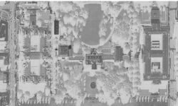
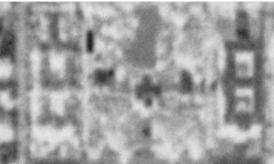
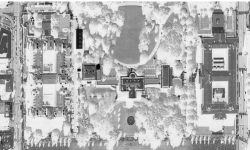
To fix ideas, we introduce a typical instance where the observations form a a sequence of resolution limited inverse problems. During satellite imaging operations, a location on Earth is imaged many times over the life span of the satellite. The quality of the recorded observations can be low and variable due to changing atmospheric and/or weather conditions. See the left column of Figure 1 for a representative panel of four such images taken of the White House and surrounding buildings. Note that the amount of blurring in each image $i$, corresponding to the forward operators $K_{i}$, can be very different. However, the pixelization induced by the observational device is fixed over the sequence of images.

Our proposed estimator $\hat{\theta}_{n}$ takes these images and sequentially creates a new estimate of the unknown signal $\theta$ after each observation $Y_{i}$ (right column of Figure 1). Each row of Figure 1 is a new observation and $\hat{\theta}_{n}$ after being updated with that observation. Notice that the recovery is quite good, even after only a few images as input. We emphasize that there are no choices to be made by the data analyst: all tuning parameters are chosen in an automatic, data-dependent way.

(a)

(b)

(c)

(d)

(e)

(f)

(g) Observations

(h) Estimates

Figure 1: Example of images of the White House from a satellite and associated recovery of the unknown signal $\theta$ using our proposed estimator. In the left column (Observations) the different amounts of blurring are due to varying atmospheric conditions and correspond to the forward operators $K_{i}$ in equation (1). In the right column (Estimates) we report the output of our estimator using the data in the left column. Each row corresponds to making another observation $Y_{i}$ and updating our estimator with this new data. We emphasize that there are no choices to be made by the data analyst; all tuning parameters are chosen in an automatic, data-dependent way.

This paper is organized as follows. In Section 2 we give a careful overview of our method and provide justification for the assumptions made, with greater exposition occurring in Appendix A. In Theorem 2.3 and Theorem 6, we give supporting theory for our estimator that both shows uniform consistency over the parameter space and an asymptotic oracle inequality. These results show both that our estimator will get the correct answer eventually, no matter the signal in our parameter space, and that our estimator makes essentially as efficient use of the data as if we knew the signal $\theta$. In Section 4, we provide an example of our framework in action on simulated data.

Notation. For $A\in\mathbb{C}^{p\times p}$ and $a\in\mathbb{C}$, define $A^{*}$ to be the Hermitian adjoint of $A$. Correspondingly, define $|a|^{2}=a^{*}a$ and $|A|^{2}=A^{*}A$ to be the squared complex modulus of a scalar and matrix, respectively. Likewise, for any vector $x\in\mathbb{C}^{p}$, $||x||^{2}=x^{*}x$. If $AA^{*}=I_{p}=A^{*}A$, then we say that $A$ is unitary. We utilize bold faced font for vectors: $\mathbf{b}_{n}\in\mathbb{C}^{p}$ with its $j^{th}$ entry notated $b_{nj}$ and the subscript $n$ indicates dependence on the sample size. Similarly, $A_{nj}$ is the $j^{th}$ element of the main diagonal of the matrix $A_{n}$. We abuse notation slightly by using $\boldsymbol{\lambda}$ as both a vector in $\mathbb{C}^{p}$ and as a function from $\mathbb{C}^{p}$ to $\mathbb{C}^{p}$ given by component-wise multiplication.

2 Methodology and main results

We begin this section by making the following assumptions, building on the notation introduced in equation (1):

• The noise parameter $\varepsilon>0$ is known.

• The $(K_{i})_{i=1}^{n}$ are known smoothing matrices.

• There exists a unitary matrix $\Psi\in\mathbb{C}^{p\times p}$ and diagonal matrices $D_{i}$ such that $K_{i}=\Psi D_{i}\Psi^{*}$ for all $i=1,\ldots,n,\ldots$.

• There exists an $N<\infty$ such that for all $j$ there exists an $1\leq i_{*}\leq N$ such that $|D_{i_{*}j}|>0$.

• Define $\Delta_{n}:=\sum_{i=1}^{n}|D_{ij}|^{2}$. Then the $(D_{i})$ are such that

  $$\lim_{n\rightarrow\infty}\frac{\max_{j}\Delta_{nj}}{\min_{j}\Delta_{nj}}<\infty.$$

Assumptions (A1) and (A2) are very standard in the statistical inverse problem literature. We discuss a strategy for estimating $\varepsilon$ in Section 3.2. Assumption (A4) is also commonly made and it ensures that, at some point, the entire signal $\theta$ is identified and loosely corresponds to the intersection of the null spaces of the $(K_{i})_{i=1}^{n}$ eventually only containing the zero vector. Assumption (A5) merely prevents a pathological case where the $K_{i}$ are becoming more ill-conditioned without bound as $n\rightarrow\infty$. Assumption (A3) is crucial to our method and while the reason for it will become clear, the following theorem provides a general family of matrices that satisfy it:

Theorem 2.2.

If the $(K_{i})_{i=1}^{n}$ all correspond to the convolution operation, then there exists a unitary matrix $\Psi$ and a sequence of diagonal matrices $(D_{i})_{i=1}^{n}$, all of which could have complex entries, such that (A3) holds. If $\theta$ is a one (two)-dimensional signal, then the $K_{i}$ are (block) circulant and the entries of the matrix $\Psi$ are the discrete one (two)-dimensional Fourier basis and the entries of $D_{i}$ are the corresponding discrete one (two)-dimensional Fourier coefficients.

Hence, we see that (A3) is more general than the convolutional assumption made in Piana and Bertero (1996) and many other works concerning statistical inverse problems. See Appendix A for a proof of Theorem 2.2 and an investigation into more general families of matrices that satisfy assumption (A3).

2.1 Overview and main results

An overview of our procedure is as follows. The parameter $\theta$ and each observation $\mathbf{Y}_{i}$ us rotated by $\Psi^{*}$. The rotated $\mathbf{Y}_{i}$’s are combined together to form a sufficient statistic $\mathbf{B}_{n}$. The estimators we consider are of the form $\hat{\theta}=\Psi\boldsymbol{\lambda}(\mathbf{B}_{n}):=\Psi(\lambda_{j}B_{nj})_{j=1}^{p}$. Define this set of estimators to be

$$\mathcal{E}=\{\hat{\theta}=\Psi\boldsymbol{\lambda}(\mathbf{B}_{n}):\boldsymbol{\lambda}\in\mathbb{C}^{p}\}.$$ (2)

We choose from the estimators in $\mathcal{E}$ using a combination of minimizing an empirical estimator of the risk and some additional regularization parameters. Define our estimator to be $\hat{\theta}_{n}=\Psi\hat{\boldsymbol{\lambda}}(B_{n})$, where

$$\hat{\lambda}_{j}=\left(1-\frac{\Omega_{n}^{2}\varepsilon^{2}}{\Delta_{nj}|B_{nj}|^{2}}\right)_{+}.$$ (3)

The form of this estimator is derived in the text containing and preceding equation (20). We set $\Omega_{n}^{2}:=(p-2)\left(1+\frac{\max_{j}\Delta_{nj}}{\min_{j}\Delta_{nj}}\right)$. Note this choice of $\Omega_{n}^{2}$ is motivated by Brown, Nie and Xie (2011) in which it is shown that ensemble minimaxality in the heteroscedastic case holds for the soft thresholded James-Stein type estimator.

We define our loss function to be the $l^{2}$ norm with associated risk

$$R(\hat{\theta},\theta):=\mathbb{E}||\hat{\theta}-\theta||^{2}$$ (4)

and set $\Theta:=\{\theta:||\theta||_{2}^{2}\leq T^{2}\}$ for any $0<T^{2}<\infty$. Then

Theorem 2.3.

Under assumptions (A1) - (A5),

$$\limsup_{n\rightarrow\infty}\,\sup_{\theta\in\Theta}\,\gamma_{n}^{-1}R\left(\hat{\theta}_{n},\theta\right)<C<\infty$$ (5)

where

$$\gamma_{n}=\max_{j}\frac{\varepsilon^{2}}{\Delta_{nj}}.$$

If $D_{ij}\equiv D_{j}$ for some $D_{j}\in\mathbb{C}$, then $\gamma_{n}\asymp 1/n$; that is the parametric rate. However, the forward operators $(K_{i})$ in effect ensure that each observation doesn’t decrease the risk equally. The quantity $\Delta_{nj}$ relates to how much information is present in the first $n$ observations about the $j^{th}$ component of $\Psi^{*}\theta$.

Additionally, we can compare our estimator to the $\mathcal{E}$-oracle $\theta_{*}$

Theorem 2.4.

Suppose assumptions (A1) - (A5) and let

$$R(\theta_{*},\theta):=\min_{\hat{\theta}\in\mathcal{E}}R(\hat{\theta},\theta)$$

be the risk of the $\mathcal{E}$-oracle. Then

$$R\left(\hat{\theta}_{n},\theta\right)\leq R(\theta_{*},\theta)(1+O(1)),$$ (6)

where the term $O(1)$ does not depend on $\theta$.

An interesting extension of this model is to the random operator setting. That is, what is the impact of having $K_{i}$ being drawn from some distribution? We answer this question in an interesting case.

2.2 Random Eigenvalues

Suppose that the $(K_{i})$ are random operators such that $K_{i}=\Psi D_{i}\Psi^{*}$ for all $i=1,2,\ldots$ and $\text{diag}(D_{i})\stackrel{{\scriptstyle i.i.d}}{{\sim}}\mathcal{D}$, where $\mathcal{D}$ is any $p$-variate complex distribution that doesn’t have too much mass near zero. Specifically,

• The distribution $\mathcal{D}$ is such that there exists an $a$ where for $0\leq\tau\leq a$

  $$\mathbb{P}_{\mathcal{D}}\left(|D_{1j}|^{2}<\tau\right)=(\tau)^{\rho}.$$

This is a stochastic extension of assumption (A4) as it allows the random eigenvalues to be arbitrarily close to zero in magnitude but with the probability of them being small going to zero at an appropriate rate. Lastly, let $(W_{i})$ and $(D_{i})$ be mutually independent.

Theorem 2.5.

Suppose assumption (B4) holds with some $\rho>1$. Then

$$\lim_{n\rightarrow\infty}\sup_{\theta\in\Theta}\mathbb{E}_{(D_{i}),(Y_{ij})}\left|\left|\hat{\theta}_{n}-\theta\right|\right|^{2}=0$$ (7)

where $\mathbb{E}_{(D_{i}),(Y_{ij})}$ corresponds to integration with respect to the joint distribution of $(D_{i})$ and $(Y_{ij})$.

2.3 Rotations, estimators, and tuning parameter selection

Returning to equation (1), for $i=1,2,\ldots$ we define $\mathbf{X}_{i}:=\Psi^{*}\mathbf{Y}_{i}$, $\beta:=\Psi^{*}\theta$, and $\mathbf{Z}_{i}:=\Psi^{*}\mathbf{W}_{i}$. Then it follows that

$$\mathbf{X}_{i}=D_{i}\beta+\varepsilon\mathbf{Z}_{i}.$$ (8)

Note that in this case $\mathbf{Z}_{i}\stackrel{{\scriptstyle i.i.d}}{{\sim}}CN(0,I_{p},\Psi\Psi^{\top})$. It is also convenient to look at equation (8) component-wise,

$$X_{ij}=D_{ij}\beta_{j}+\varepsilon Z_{ij}$$ (9)

for $j=1,\ldots,p$. Note that for these multiplications to be defined, we have to think about $\mathbb{R}^{p}$ being embedded in $\mathbb{C}^{p}$ by having imaginary part equal to zero. We follow this convention without comment in what follows.

Remark 2.6.

Note that the $(\mathbf{Z}_{i})$ are degenerate complex Gaussian vectors in the following sense: if we think of a $p$ dimensional complex Gaussian as a $2p$ dimensional real Gaussian with some covariance matrix, then the Gaussian actually has values in a $p$ dimensional subspace of $\mathbb{R}^{2p}$. Thus the random variables don’t have a density with respect to Lebesgue measure on the full space $\mathbb{C}^{p}$, among other complications.

Remark 2.7.

Commonly, the sequence space formulations found in equation (8) and equation (9) are accomplished by a real, orthogonal matrix instead of a complex, unitary one. Allowing for the sequence $(K_{i})_{i=1}^{n}$ to share the same eigenvectors necessitates permitting $\Psi$ to be complex. This makes equation (9) more complicated than the conventional normal means problem in at least two ways. First, as stated above, the random variables are complex. Second, and more importantly, the model is heteroscedastic. This leads to a much more involved theory than in the homoscedastic case, such as in Brown (1975), and is still the topic of contemporary research (Brown, Nie and Xie, 2011).

Lastly, define

$$B_{nj}:=\frac{\sum_{i=1}^{n}D_{ij}^{*}X_{ij}}{\sum_{i=1}^{n}|D_{ij}|^{2}}=\beta_{j}+\varepsilon\Delta_{nj}^{-1/2}Z_{j}$$ (10)

where $\Delta_{nj}:=\sum_{i=1}^{n}|D_{ij}|^{2}$.

This quantity is particularly important, as evidenced by the following theorem

Theorem 2.8.

Under the model introduced in equation (1) and (A1) - (A4), the random vector $\mathbf{B}_{n}:=(B_{nj})_{j=1}^{p}$ is sufficient for $\beta$ in equation (8).

This claim can be seen by noting that the map $\Phi^{*}$ is measure preserving.

As $\Psi$ is also unitary, we can define an equivalent risk to the one defined in equation (4) in terms of $\beta$

$$R(\hat{\theta},\theta):=\mathbb{E}||\hat{\theta}-\theta||^{2}=\mathbb{E}||\Psi^{*}(\hat{\theta}-\theta)||^{2}=\mathbb{E}||\hat{\beta}-\beta||^{2}=:R(\hat{\beta},\beta).$$ (11)

Any risk computations made under the data, which is $(X_{i})_{i=1}^{n}$ in our notation, are equivalent to those made under a sufficient statistic (Bahadur, 1954, Theorem 7.1). By Theorem 2.8, $\mathbf{B}_{n}$ is sufficient for $\beta$ and hence for all measurable functions of the data that are not functions of $\mathbf{B}_{n}$, there exists an estimator with equal risk that is a function of $\mathbf{B}_{n}$. In fact, the expectations in equation (11) are equivalent under $(X_{i})_{i=1}^{n}$ and $\mathbf{B}_{n}$. Therefore, for each $n$, we can treat $\mathbf{B}_{n}$ as the data and formulate estimators based upon it.

To develop an automatic procedure for signal estimation in sequential inverse problems we begin by regularizing an unbiased estimator of $\beta$ through the use of a smoothing parameter vector. We choose this smoothing parameter by minimizing an estimate of the risk. This type of procedure, known generally as unbiased risk estimation, has been revisited regularly in many fields for solving various problems related to denoising (Stein, 1981; Donoho and Johnstone, 1995). However, as inverse problems generally result in unstable estimators of both the parameter $\beta$ and the risk $R$, we compensate by including additional regularization.

The specifics of our approach are related to the procedure found in Beran (2000). However, the goal in Beran (2000), unlike our paper, is the estimation of the regression function in an assumed linear model instead of the coefficients themselves. That is, referring to the notation in equation (1), the estimation of $K_{i}\theta$ instead of the estimation of $\theta$. This is an important distinction as both estimating $\theta$ is intrinsically harder than estimating $K_{i}\theta$ and $\theta$ is the object of actual interest. The practical implications of these differences is that only minimizing an unbiased estimate of risk, as is the procedure in Beran (2000), provides insufficient regularization. As well, the theoretical justification that appears in Beran (2000), is essentially entirely asymptotic in $p$. This is a regime we do not consider relevant for the problem at hand.

To begin to formulate an estimator of $\beta$, and therefore $\theta$, we state the following:

Proposition 2.9.

Define $\hat{\psi}_{j}:=(|B_{nj}|^{2}-\varepsilon^{2}/\Delta_{nj})/|B_{nj}|^{2}$. Then the random function

$$\hat{R}_{n}(\boldsymbol{\lambda}):=\sum_{j=1}^{p}(\lambda_{j}-\hat{\psi}_{j})^{2}|B_{nj}|^{2}$$ (12)

provides, up to a constant independent of $\boldsymbol{\lambda}$, an unbiased estimate of $R(\boldsymbol{\lambda})$. Additionally,

$$\min_{\lambda\in\mathbb{C}^{p}}R(\boldsymbol{\lambda})=\min_{\lambda\in\mathcal{L}}R(\boldsymbol{\lambda})$$ (13)

where $\mathcal{L}=[0,1]^{p}$ is the $p$ dimensional hypersquare.

The first part of the proposition provides an unbiased estimate of the risk while the second part implies that we gain no improvement in risk by allowing $\boldsymbol{\lambda}$ to have values outside of $\mathcal{L}$.

Using $\hat{R}_{n}$ from (12), define for any $\mathcal{G}\subseteq\mathcal{L}$

$$\hat{\boldsymbol{\lambda}}^{\mathcal{G}}:=\operatorname*{\arg\!\min}_{\mathcal{G}}\hat{R}_{n}(\boldsymbol{\lambda})$$ (14)

which produces an estimator of $\beta$ via

$$\hat{\beta}^{\mathcal{G}}:=\hat{\boldsymbol{\lambda}}^{\mathcal{G}}(\mathbf{B}_{n}).$$ (15)

Lastly, we recover an estimate of $\theta$ by forming $\hat{\theta}^{\mathcal{G}}:=\Psi\hat{\beta}^{\mathcal{G}}$.

As any choice of $\mathcal{G}$ results in an estimator $\hat{\beta}^{\mathcal{G}}$ via the above machinery, there are in principle many possible choices. We focus on $\mathcal{G}=\mathcal{L}$, which by inspection of equation (12), results in

$$\hat{\boldsymbol{\lambda}}^{\mathcal{L}}=\left(1-\frac{\varepsilon^{2}}{\Delta_{nj}|B_{nj}|^{2}}\right)_{+}$$ (16)

where as usual $(\cdot)_{+}=\max(\cdot,0)$ is the soft thresholding function. Other choices can and should be explored in further research into estimation in sequential inverse problems such as $\mathcal{M}:=\{\boldsymbol{\lambda}\in\mathcal{L}:\lambda_{1}\geq\lambda_{2}\geq\ldots\geq\lambda_{p}\}$, which induces a monotonicity constraint on the estimated coefficients, or block methods of piecewise constant weights (Cavalier and Tsybakov, 2002).

Additionally, the aforementioned Tikonov-Phillips regularization and Landwieber iterations methods correspond to specific subsets of $\mathcal{L}$. The Tikonov-Phillips estimator takes the form

$$\hat{\beta_{j}}^{\gamma}:=\sum_{i=1}^{n}\frac{D_{ij}^{*}X_{ij}}{|D_{ij}|^{2}+\gamma}$$ (17)

which can be rewritten as an element of $\mathcal{E}$ by defining

$$\lambda_{j}^{\gamma}:=\frac{\Delta_{nj}}{\Delta_{nj}+\gamma}$$ (18)

with associated estimator $\hat{\beta}^{\gamma}=\boldsymbol{\lambda}^{\gamma}(\mathbf{B_{n}})$.

The Landwieber iterations estimator is by nature iterative. However, it has an equivalent formation in the form of the following linear smoother

$$\lambda_{j}^{(\gamma,\tau)}=(1-[1-\tau\Delta_{nj}]^{\gamma})$$ (19)

where $\gamma$ corresponds to the number of iterations and $\tau$ is a relaxation parameter. The associated estimator is $\hat{\beta}^{(\gamma,\tau)}=\boldsymbol{\lambda}^{(\gamma,\tau)}(\mathbf{B}_{n})$. Hence, this procedure generalizes the results in Piana and Bertero (1996) by providing a principled tuning parameter selection method.

A problem arises if we choose smoothing parameters in this fashion in inverse problems: insufficient regularization. This is due to $\hat{R}_{n}$ being an unstable estimate of $R$ for the same reason as $\mathbf{B}_{n}$ is an unstable estimator of $\beta$.

Instead of regularizing the risk estimator, we modify the weights directly to provide additional regularization. However, we record our belief that regularizing $\hat{R}_{n}$ by limiting how ill-conditioned the risk estimator can become and then minimizing this biased estimator of the risk should provide a suite of interesting estimators via the above machinery. Define

$$\hat{\boldsymbol{\lambda}}=\left(1-\frac{\Omega_{n}^{2}\varepsilon^{2}}{\Delta_{nj}|B_{nj}|^{2}}\right)_{+}$$ (20)

where the parameter $\Omega_{n}^{2}$ is specified before Theorem 2.3. Lastly, define our estimator of $\theta$ to be

$$\hat{\theta}_{n}:=\Psi\hat{\boldsymbol{\lambda}}(\mathbf{B}_{n}).$$ (21)

3 Computational concerns, variance estimation, and alternate methods

3.1 Computations

The specifics of the computation of an estimator $\hat{theta}^{\mathcal{G}}$ depend on the subset $\mathcal{G}$. However, $\hat{R}_{n}$ is a convex objective function. Hence, if $\mathcal{G}$ is a convex subset of $\mathbb{R}^{p}$, then the solution can be found both efficiently and uniquely. Of the estimators mentioned above, all except $\mathcal{M}$ have a closed form solution and therefore trivial computation. The minimization of $\hat{R}_{n}$ over $\mathcal{M}$ can be accomplished by a well known algorithm called Pooled Adjacent Violators (PAV) (Robertson, Wright and Dykstra, 1988) that transforms the least squares solution $\hat{\psi}$ into the monotone solution by taking weighted averages of adjacent elements of $\hat{\psi}$ that violate the monotonicity constraint.

Additionally, in the case of convolution, the vector $\Delta_{n}$ and the random variables $(X_{i})$ can be computed via the Fast Fourier Transform, which implies $O(p\log p)$ computations and is of course the archetypal instance of an efficient algorithm. However, for more general matrices $K_{i}$, the eigenvectors must be computed via a conventional eigenvector solver, which necessarily has computational complexity $O(p^{3})$. This could become prohibitive for large scale problems. There do exist modern approximation methods for eigenvalues and eigenvectors that could be used instead, such as in Halko, Martinsson and Tropp (2009). However, we do not explore this idea further in this paper.

An additional feature is that for the computation at step $n$, it is not necessary to keep the entire history $(Y_{i})_{i=1}^{n}$ and $(K_{i})_{i=1}^{n}$. Both $\mathbf{B_{n}}$ and $\Delta_{n}$ can be computed from aggregate information. Hence, we can produce an estimate of $\theta$ given only access to a few summary statistics which get updated after each new observation.

3.2 Estimating the variance parameter

Estimating the variance parameter can be accomplished in a consistent way by setting aside a subsequence $\mathcal{N}$ of $\mathbb{N}$ and computing the estimator

$$\hat{\varepsilon}_{\text{con}}^{2}:=\frac{1}{pn^{\prime}}\sum_{i\in\mathcal{N}}\sum_{j=1}^{p}\left(Y_{ij}^{2}-\overline{Y}_{j}^{2}\right).$$ (22)

Here, we have computed the estimator after the first $n^{\prime}$ entries in $\mathcal{N}$.

Alternatively, we can take advantage of the observational process to acquire a good estimate of $\epsilon$. As we make observations, occasionally some will be of exceptionally poor quality. This observation will be less helpful for recovery in general and provide almost no information about the higher order components of the vector $\beta$.

Suppose now that $\mathcal{N}$ is the set of all indices $i$ such that $Y_{i}$ is a low quality observation; that is there exists a $p^{\prime}$ such that for $j=p^{\prime},\ldots,p$, the $|D_{ij}|^{2}$ are small. In general, $p^{\prime}$ could depend on $i$, but we do not consider this complication here. Form the following statistic

$$\hat{\varepsilon}_{i}^{2}:=\frac{1}{p-p^{\prime}}\sum_{q=p^{\prime}}^{p}|X_{iq}|^{2}.$$ (23)

Then $\mathbb{E}\hat{\varepsilon}_{i}^{2}=\varepsilon^{2}+\frac{1}{p-p^{\prime}}\sum_{q=p^{\prime}}^{p}|D_{iq}|^{2}|\beta_{j}|^{2}$ and we report $1/n^{\prime}\sum_{i\in\mathcal{N}}\hat{\varepsilon}_{i}^{2}$ as our estimator of $\epsilon^{2}$. This is in general a biased estimator of the variance. Nevertheless, it is still useful. First, it is conservative owing to its positive bias. Perhaps more importantly, this estimator provides an interesting situation where the lowest quality parts of the lowest quality observations provide the best performance.

3.3 Averaging is not enough

In equation (1), conventional statistical practice would suggest averaging the observations $(Y_{i})$ directly. However, we show here that this leads to suboptimal results. Specifically, averaging gives thes following model

$$\overline{Y}_{n}=\overline{K}_{n}\theta+\frac{\varepsilon}{\sqrt{n}}W$$ (24)

where, under assumption (A3), $\overline{K}_{n}:=1/n\sum_{i=1}^{n}K_{i}=\Psi\overline{D}_{n}\Psi^{*}$,
$\overline{D}_{n}:=1/n\sum_{i=1}^{n}D_{i}$, $\overline{Y}_{n}:=1/n\sum_{i=1}^{n}Y_{i}$, and $W\sim N(0,I_{p})$. This can also be equivalently expressed as

$$\overline{\mathbf{B}}_{n}=|\overline{D}_{n}|^{-2}\overline{D}_{n}^{*}\overline{X}_{n}=\beta+\frac{\varepsilon}{\sqrt{n}}|\overline{D}_{n}|^{-2}\overline{D}_{n}^{*}\Psi^{*}W.$$ (25)

Here, $\overline{X}_{n}=\Psi^{*}\overline{Y}_{n}$. We define the corresponding set of linear estimators to be $\overline{\mathcal{E}}:=\{\hat{\theta}=\Psi\boldsymbol{\lambda}(\overline{\mathbf{B}}_{n}):\boldsymbol{\lambda}\in\mathbb{C}^{p}\}$.

Note that we can write equation (24) without any assumptions about the eigenvectors of the forward operators. However, under assumption (A3), the following theorem supports forming estimators based on equation (10) instead of equation (24).

Theorem 3.10.

Suppose for a fixed $\theta$,

$$R_{1}=\inf_{\hat{\theta}\in\mathcal{E}}\mathbb{E}||\hat{\theta}-\theta||_{2}^{2}\quad\text{ and }\quad R_{2}=\inf_{\hat{\theta}\in\overline{\mathcal{E}}}\mathbb{E}||\hat{\theta}-\theta||_{2}^{2},$$

where the expectations in $R_{1}$ and $R_{2}$ are under $\mathbf{B}_{n}$ and $\overline{\mathbf{B}}_{n}$, respectively. Then

$$R_{1}<^{*}R_{2}$$

where ‘$<^{*}$’ means ‘strictly less than except when $D_{i}\equiv D$ for all $i$ and some $D$.’ That is, the oracle linear risk based on equation (10) is strictly less than the oracle linear risk based on equation (24).

Remark 3.11.

Note that the classic Tikonov-Phillips estimator based on the $\overline{Y}_{n}$ is of the form

$$\hat{\theta}_{\text{ridge}}=(\overline{K}_{n}^{\top}\overline{K}_{n}+\tau I)^{-1}\overline{K}_{n}^{\top}\overline{Y}_{n}.$$

This is equivalent to

$$\hat{\theta}_{\text{ridge}}=\Psi(|\overline{D}_{n}|^{2}+\tau I)^{-1}|\overline{D}_{n}|^{2}|\overline{D}_{n}|^{-2}\overline{D}_{n}^{*}\overline{X}_{n}=\Psi(|\overline{D}_{n}|^{2}+\tau I)^{-1}|\overline{D}_{n}|^{2}\overline{\mathbf{B}}_{n},$$ (26)

and hence the Tikonov-Phillips estimator is in $\overline{\mathcal{E}}$, among many others.

An alternative approach relies on forming $\mathcal{K}_{n}:=[K_{1}^{\top},\ldots,K_{n}^{\top}]^{\top}$, $\mathcal{Y}_{n}:=[Y_{1}^{\top},\ldots,Y_{n}^{\top}]^{\top}$, and $\mathcal{W}_{n}\sim N(0,I_{np})$. Then it follows that

$$\mathcal{Y}_{n}=\mathcal{K}_{n}\theta+\varepsilon\mathcal{W}_{n}.$$ (27)

However, estimators based on this approach, such as spline type estimators, rely on accessing the entire history of observations $(Y_{i})$ and forward operators $(K_{i})$. This is computationally infeasible as this means both keeping and repeatedly accessing the entire sequence of observations. Hence, this approach doesn’t satisfy our requirement of an estimate at time $n$ being efficiently updatable to a new estimate after recording $Y_{n+1}$.

4 Supporting simulations

4.1 Description

In this section we present visual results of using our estimator $\hat{\theta}_{n}$ to reconstruct various signals, given access only to smoothed and noisy, but repeated, observations of that signal. In both cases, we compare our estimator, $\hat{\theta}_{n}$ to $\hat{\theta}_{\text{ridge}}$ from equation (26), with the smoothing parameter $\tau$ chosen by minimizing generalized cross validation (GCV). For a quantitative comparison, we use the normalized relative risk ($RR$) given by

$$RR(\hat{\theta},\theta)=\sqrt{\frac{R(\hat{\theta},\theta)}{||\theta||^{2}}}.$$ (28)

We estimate $RR$ by averaging 100 runs of our simulations.

For each of the signals introduced below, we set $p=256$ and fix the noise parameter $\epsilon$ to be such that the signal-to-noise $:=||\theta||_{1}/(p\epsilon)=1$. For these examples, we admit $K_{i}$ that are an equally weighted mixture of three Gaussians, normalized to have $l_{1}$ mass equal to 1, with means $\mu_{1}=-0.75$, $\mu_{2}=0.00$, and $\mu_{3}=0.50$, along with standard deviations $\sigma_{iq}=0.5+E_{qi}$, where $E_{qi}\stackrel{{\scriptstyle i.i.d.}}{{\sim}}\text{exponential}(1)$ and $q=1,2,3$. Note that this implies that the $K_{i}$ are not symmetric. Also, note that Gaussian-like smoothing represents one of the worst cases as it exponentially down-weights the $\beta_{j}$ for large $j$.

(a)

(b)

(c)

(d)

Figure 2: The left column corresponds to $\theta^{\text{smooth}}$ and the right column corresponds to $\theta^{\text{peaked}}$. The top row is a plot of the signal itself, along with the signal after the minimum (dashed line) and maximum (dashed and dotted line) amount of smoothing. The bottom row is an example of the recorded data after corruption by smoothing and noise. Notice that in $\theta^{\text{peaked}}$, the smaller peak is completely obscured.

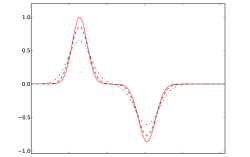
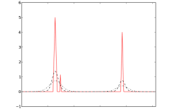
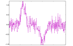
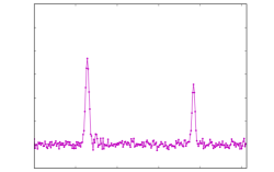
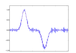
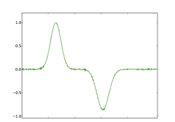
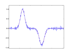
We consider two signals for estimation, which we refer to as $\theta^{\text{smooth}}$ and $\theta^{\text{peaked}}$ (Figure 2). The first signal, $\theta^{\text{smooth}}$, is the sum of two Gaussians functions that are filtered by a Gaussian-tapered filter. This filter is additionally enforced to be zero above the $p/2$ frequency. Hence, $\theta^{\text{smooth}}$ is very smooth and compactly supported in the frequency domain. This example is instructive as a smooth function should be well represented by the eigenvectors $\Psi$ of the smoothing operators $K_{i}$. Also, a compact representation in frequency domain will reveal the effectiveness of the soft-thresholding in zeroing out the appropriate $B_{nj}$, ie: those that correspond to the $\beta_{j}$ that are zero. See the left column of Figure 2 for a plot of $\theta^{\text{smooth}}$ (top) along with a typical example of a noisy, smoothed version that comprises the recorded data (bottom).

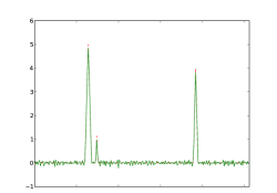
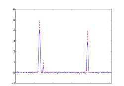
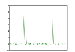
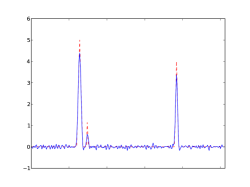
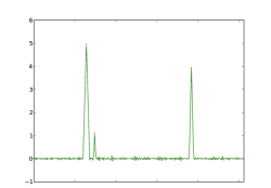
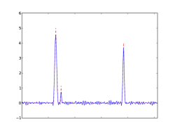
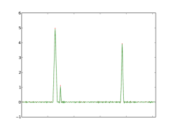
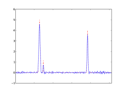
Additionally, we consider the opposite situation by defining a signal $\theta^{\text{peaked}}$ that is the sum of three sharp, non-smooth, peaks. This signal is difficult to represent with the eigenvectors of smoothing matrices but is common in signal processing as it corresponds to both spectra from biochemical analysis and nuclear magnetic resonance imaging (nMRI). Note that the smallest peak is completely obscured by the smoothing and noise. See the right column of Figure 2 for a plot of $\theta^{\text{peaked}}$ (top) along with an example of a noisy, smoothed version (bottom).

4.2 Results

In estimating either signal, $\theta^{\text{smooth}}$ or $\theta^{\text{peaked}}$, the estimator $\hat{\theta}_{n}$ converges rapidly to the truth. See Table 1 for the $RR$ of $\hat{\theta}_{n}$ and $\hat{\theta}_{\text{ridge}}$ used on both signals. In each case, for $n=50$, the $RR$ are approximately the same, with $\hat{\theta}_{\text{ridge}}$ having a slight edge. Every sample size thereafter shows substantial advantage of $\hat{\theta}_{n}$ over $\hat{\theta}_{\text{ridge}}$, culminating with a factor of two improvement in $RR$ after $n=300$ observations.

For estimating $\theta^{\text{smooth}}$, both estimators have substantial oscillations for low sample sizes. However, due to $\hat{\theta}_{n}$ having a soft-thresholding effect, some of the entries in our estimator of $\beta$ are zeroed out. In contrast, $\hat{\theta}_{\text{ridge}}$ only shrinks the coefficients and hence still has substantial fluctuations after $n=300$ observations. See Figure 3 for graphical results.

(a)

(b)

(c)

(d)

(e)

(f)

(g) $\hat{\theta}_{n}$

(h) $\hat{\theta}_{\text{ridge}}$

Figure 3: Estimation of $\theta^{\text{smooth}}$ by $\hat{\theta}_{n}$ (left column) and $\hat{\theta}_{\text{ridge}}$ (right column). The sample sizes range from top to bottom, $n=50,100,200,300$. Our estimator, $\hat{\theta}_{n}$, quickly converges to $\theta^{\text{smooth}}$. However, $\hat{\theta}_{\text{ridge}}$, which doesn’t zero out any coefficients, still has substantial fluctuations after $n=300$ observations. See Table 1 for $RR$ results for this simulation.

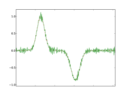
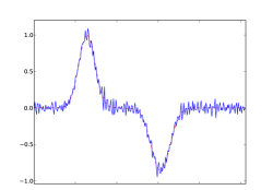
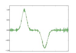
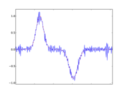
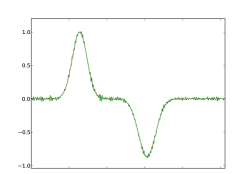
For the signal $\theta^{\mathrm{peaked}}$, $\hat{\theta}_{n}$ estimates the true height of the peaks accurately and quickly. In particular, the secondary small peak is definitively identified with the correct shape and height for $n=50$ observations, while for $\hat{\theta}_{\text{ridge}}$, the secondary peak is much less clear. There are still some remaining oscillations at $n=300$, resulting from unavoidable consequence of using the eigenvector basis. This is a well-known phenomenon in Fourier analysis known as the ‘Gibbs effect.’ Even with this obstacle, $\hat{\theta}_{n}$ converges quickly to $\theta^{\mathrm{peaked}}$. See Figure 4 for graphical results.

(a)

(b)

(c)

(d)

(e)

(f)

(g) $\hat{\theta}_{n}$

(h) $\hat{\theta}_{\text{ridge}}$

Figure 4: Estimation of $\theta^{\mathrm{peaked}}$ by $\hat{\theta}_{n}$ (left column) and $\hat{\theta}_{\text{ridge}}$ (right column). The sample sizes range from top to bottom, $n=50,100,200,300$. Our estimator, $\hat{\theta}_{n}$, estimates the true height of the peaks accurately and quickly. In particular, the secondary small peak is definitively identified with the correct shape and height. There are still some remaining oscillations at $n=300$, resulting from an unavoidable Gibbs effect from using the eigenvectors as a basis. See Table 1 for $RR$ results for this simulation.

	$RR(\hat{\theta}_{n},\theta^{\text{smooth}})$	$RR(\hat{\theta}_{\text{ridge}},\theta^{\text{smooth}})$	$RR(\hat{\theta}_{n},\theta^{\text{peaked}})$	$RR(\hat{\theta}_{\text{ridge}},\theta^{\text{peaked}})$
$n=50$	0.291	0.288	0.148	0.151
$n=100$	0.210	0.223	0.116	0.171
$n=200$	0.149	0.199	0.092	0.149
$n=300$	0.120	0.173	0.079	0.141

Table 1: The $RR$ for the two considered simulations. These are estimated by averaging 100 runs of our simulations.

5 Discussion

In this paper, we provide a general method for recovering an unknown signal given a sequence of noisy observations that are only indirectly of that signal of interest. Our estimator, $\hat{\theta}_{n}$, has many favorable properties. It has computational efficiency in the sense that it can be updated with a new observation without need to reference the entire sequence of observations. Instead, it relies on only a few summary statistics that need to be maintained and updated. Though its computation is predicated on finding the eigenvectors and eigenvalues of potentially large matrices, the implementation is straightforward and generalizable to higher dimensional signals such as images. Additionally, there exist accurate methods for the approximate computation of the eigenvectors of matrices that could in principle be used to speed up the computation of $\Psi$.

Also, $\hat{\theta}_{n}$ is statistically efficient as well. The uniform consistency and oracle inequality results show that it is making about as good a use of the data as possible. Likewise, $\hat{\theta}_{n}$ has worked very well in our experiments so far, as evidenced by the results in Figures 1, 3, and 4. Our estimator can recover the unknown signal $\theta$ efficiently, requiring very few observations. Also, referring to the second row of Figure 1, the collection of a very poor observation merely doesn’t improve the estimate instead of decreasing its quality. This is in opposition to many currently implemented techniques such as straight averaging, where low quality observations decrease the quality of the recovery.

Appendix A

This section gives warrant for assumption (A3) in Section 2. Although a slightly weaker version of assumption (A3) is all that is actually required (that only the right eigenvectors need be the same instead of both left and right eigenvectors) we leave it in its current form for simplicity of exposition and conditions.

Two real matrices $A,B$ share the same eigenvectors if they are simultaneously unitarily diagonalizable; that is, there exists two diagonal matrices $\Sigma_{1},\Sigma_{2}$ and an unitary matrix $\Psi$ such that $A=\Psi\Sigma_{1}\Psi^{*}$ and $B=\Psi\Sigma_{2}\Psi^{*}$. Note $A$ and $B$ must of course be unitarily diagonalizable, which implies by the spectral theorem that $A$ and $B$ are normal; that is $A^{\top}A=AA^{\top}$ and $B^{\top}B=BB^{\top}$. The following theorem characterizes simultaneous diagonalizability.

Lemma A.12.

Let $\mathcal{K}$ be a commuting family of normal matrices. Then $\mathcal{K}$ is also simultaneously unitarily diagonalizable.

Proof A.13 (Proof of Lemma A.12).

By the Schur unitary triangularization theorem (Horn and Johnson, 1985, Theorem 2.3.1) if $\mathcal{K}$ is a commuting family of matrices, then there is a unitary $\Psi$ such that $\Psi K\Psi^{*}$ is upper triangular for every $K\in\mathcal{K}$. Hence, as normality is preserved under unitary congruence and a triangular normal matrix must be diagonal, the result follows.

Though all Toeplitz matrices commute asymptotically as the number of rows and columns increases, not all Toeplitz matrices commute for a fixed size. Many subsets of the family of Toeplitz matrices satisfy Lemma A.12, however. In particular, all circulant matrices commute (Gray, 2001, Chapter 3.1). This shows Theorem 2.2.

Appendix B

We utilize the following notation in several of the below proofs. We use $\lesssim$ to indicate ‘less than or equal to up to a constant independent of $n$.’ Also, it is convenient to think of a complex number $a=a_{1}+a_{2}i$ as an element $(a_{1},a_{2})\in\mathbb{R}^{2}$. In this case, we use $|||a|||^{2}=a_{1}^{2}+a_{2}^{2}$ as a norm on $\mathbb{R}^{2}$, as the complex modulus is not technically defined on elements of $\mathbb{R}^{2}$. Additionally, $Z\sim N(0,I_{2})$ is the two dimensional standard normal. Lastly, we define $s_{nj}:=\Omega_{n}^{2}\varepsilon^{2}/\Delta_{nj}$.

We begin with a lemma that will be used in the proofs of Theorem 2.3 and Theorem 6:

Lemma B.14.

Let $\mu\in\mathbb{R}^{2}$ be a vector, $\Sigma=$ diag$(\sigma_{1}^{2},\sigma_{2}^{2})$ be a diagonal matrix with positive entries, and $c^{2}$ be a real, positive constant. Then

$$\mathbb{P}(|||\mu+\Sigma^{1/2}Z|||^{2}\leq c^{2})\leq\mathbb{P}(|||\mu+\sigma_{\text{max}}Z|||^{2}\leq c^{2})$$ (29)

if $|||\mu|||>c$ and $\sigma_{\text{max}}=\max\{\sigma_{1},\sigma_{2}\}$.

Here, we don’t give a formal proof but provide intuition. The probability in equation (29) corresponds to the amount of the mass of an elliptical normal, aligned with the cononical axis, that resides in a ball of radius $c$ at the origin. Hence, if $|||\mu|||>c$ (that is, the mean is outside the ball) a more spread out the normal results in more mass inside the ball.

Proof B.15 (Proof of Theorem 2.3).

For simplicity, write $\hat{\beta}_{n}:=\hat{\boldsymbol{\lambda}}(\mathbf{B}_{n})$. Then

$$\sup_{\theta\in\Theta}R_{n}(\hat{\theta},\theta)=\sup_{\beta\in\mathcal{B}}R_{n}(\hat{\beta}_{n},\beta),$$

where $\mathcal{B}:=\{\beta:||\beta||^{2}\leq T^{2}\}=\Psi^{*}\Theta$. Then we wish to show that

$$\limsup_{n\rightarrow\infty}\sup_{\beta\in\mathcal{B}}R_{n}(\hat{\beta}_{n},\beta)=0,$$ (30)

where the subscript $n$ on $R$ has been included to emphasize the dependence on $n$.

We begin by defining the following set

$$A_{j}:=\{\omega:|B_{nj}(\omega)|^{2}>s_{nj}^{2}\}$$

where $\omega$ ranges over the measure space on which the random variable $B_{nj}$ is defined. The utility of defining $A_{j}$ is

$$\hat{\beta}_{nj}\mathbf{1}_{A_{j}}=\left(1-\frac{\Omega_{n}^{2}\varepsilon^{2}}{\Delta_{nj}|B_{nj}|^{2}}\right)B_{nj}\mathbf{1}_{A_{j}}$$ (31)

Additionally, write $B_{nj}=\beta_{j}+Z_{nj}$ as a mean term plus stochastic term, where $Z_{nj}$ is the $j^{th}$ entry in the complex normal $\varepsilon\Delta_{n}^{-1}\sum_{i}(D_{i}^{*}\Psi^{*}W_{i})$. Then the following bound on the $j^{th}$ term in the loss holds:

$$|\hat{\beta}_{nj}-\beta_{j}|^{2} =\mathbf{1}_{A_{j}}|\hat{\beta}_{nj}-\beta_{j}|^{2}+\mathbf{1}_{A_{j}^{c}}|\hat{\beta}_{nj}-\beta_{j}|^{2}$$

$$=\mathbf{1}_{A_{j}}\left|\left(1-\frac{s_{nj}^{2}}{|B_{nj}|^{2}}\right)B_{nj}-\beta_{j}\right|^{2}+\mathbf{1}_{A_{j}^{c}}|\beta_{j}|^{2}$$

$$=\mathbf{1}_{A_{j}}\left|Z_{nj}-\left(\frac{s_{nj}^{2}(\beta_{j}+Z_{nj})}{|\beta_{j}+Z_{nj}|^{2}}\right)\right|^{2}+\mathbf{1}_{A_{j}^{c}}|\beta_{j}|^{2}$$ (32)

$$\leq\mathbf{1}_{A_{j}}\left(|Z_{nj}|+\frac{s_{nj}^{2}}{|\beta_{j}+Z_{nj}|}\right)^{2}+\mathbf{1}_{A_{j}^{c}}|\beta_{j}|^{2}$$

$$\leq\mathbf{1}_{A_{j}}\left(|Z_{nj}|+s_{nj}\right)^{2}+\mathbf{1}_{A_{j}^{c}}|\beta_{j}|^{2}.$$

To show that the expected value of the first term goes to zero in expectation, observe:

$$\mathbb{E}\mathbf{1}_{A_{j}}\left(|Z_{nj}|+s_{nj}\right)^{2} =\mathbb{E}|Z_{nj}|^{2}+2s_{nj}\mathbb{E}|Z_{nj}|+s_{nj}^{2}$$

$$\leq\mathbb{E}|Z_{nj}|^{2}+2s_{nj}\sqrt{\mathbb{E}|Z_{nj}|^{2}}+s_{nj}^{2}$$

$$=\frac{\varepsilon^{2}}{\Delta_{nj}}+2s_{nj}\sqrt{\frac{\varepsilon^{2}}{\Delta_{nj}}}+s_{nj}^{2}$$

$$\leq\frac{\varepsilon^{2}}{\Delta_{nj}}\left(1+2\Omega_{n}+\Omega_{n}^{2}\right).$$

As $\Omega_{n}^{2}<C<\infty$ for $n$ large enough for some $C$ by assumption (A5),

$$\mathbb{E}\mathbf{1}_{A_{j}}\left(|Z_{nj}|+s_{nj}\right)^{2}=O(1/\Delta_{nj})$$ (33)

uniformly in $\beta$.

For the second term, $\mathbf{1}_{A_{j}^{c}}|\beta_{j}|^{2}$, we need to show

$$\limsup_{n\rightarrow\infty}\sup_{\beta\in\mathcal{B}}\sum_{j=1}^{p}\mathbb{P}(A_{j}^{c})|\beta_{j}|^{2}=0.$$ (34)

First, we compute the eigenvalue matrix $\Lambda_{nj}$ of the covariance matrix of $Z_{nj}$ as a vector in $\mathbb{R}^{2}$. By the properties of complex normals

$$Z_{nj}\sim N\left(\left(\begin{array}[]{c}0\\ 0\end{array}\right),\left(\begin{array}[]{ll}\varepsilon^{2}/\Delta_{nj}&\Im C_{jj}\\ \Im C_{jj}&\varepsilon^{2}/\Delta_{nj}\end{array}\right)\right)$$

where $C_{jj}$ is the $j^{th}$ diagonal entry of the matrix $\varepsilon^{2}\Delta_{n}^{-1}\sum_{i}(D_{i}^{*}\Psi^{*}\overline{\Psi}\overline{D_{i}})\Delta_{n}^{-1}$. Hence, the entries in $\Lambda_{nj}$ are $\lambda_{nj,1}^{2}=\varepsilon^{2}/\Delta_{nj}+\Im C_{jj}$ and $\lambda_{nj,2}^{2}=\varepsilon^{2}/\Delta_{nj}-\Im C_{jj}$, which are both strictly positive. Also, define $U$ to be the associated eigenvector matrix.

Though it is clear that $\mathbb{P}(A_{j}^{c})|\beta_{j}|^{2}$ goes to zero pointwise, the worst $\beta_{j}$ is arbitarily close to zero. Hence, to show uniform convergence, we define a parameter $\tau_{nj}^{2}$. For each $j$, define $\mathcal{B}_{j}:=\{\beta_{j}:|||\beta_{j}|||^{2}\leq T^{2}\}$ and split this set into $\mathcal{B}_{j}=\mathcal{B}_{jn}\cup\mathcal{B}_{jn}^{c}$, where

$$\mathcal{B}_{jn}^{c}:=\{\beta:\tau_{nj}^{2}\leq|||\beta_{j}|||^{2}\leq T^{2}\}.$$

Also, as $|||\cdot|||$ is invariant under orthogonal operations, we can rotate everything by the eigenvectors $U$. Denote rotation by $U$ by a tilde; that is, $\tilde{\beta}_{j}:=U\beta_{j}$. Then,

$$\sup_{\beta\in\mathcal{B}}\sum_{j=1}^{p}\mathbb{P}(A_{j}^{c})|\beta_{j}|^{2} \leq\sum_{j=1}^{p}\sup_{\beta_{j}\in\mathcal{B}_{j}}\mathbb{P}(A_{j}^{c})|\beta_{j}|^{2}$$

$$\leq\sum_{j=1}^{p}\max\left\{\sup_{\beta_{j}\in\mathcal{B}_{nj}}\mathbb{P}_{\beta_{j}}(A_{j}^{c})|\beta_{j}|^{2}\sup_{\beta_{j}\in\mathcal{B}_{nj}^{c}}\mathbb{P}(A_{j}^{c})|\beta_{j}|^{2}\right\}$$

$$\leq\sum_{j=1}^{p}\max\left\{\tau_{nj}^{2},\sup_{\beta_{j}\in\mathcal{B}_{nj}^{c}}\mathbb{P}(A_{j}^{c})|\beta_{j}|^{2}\right\}$$

$$=\sum_{j=1}^{p}\max\left\{\tau_{nj}^{2},\sup_{\beta_{j}\in\mathcal{B}_{nj}^{c}}\mathbb{P}(|||U(\beta_{j}+Z_{n})|||^{2}\leq s_{nj}^{2})|||\tilde{\beta}_{j}|||^{2}\right\}.$$

Then continuing on with the second term in the max, and using Lemma 29 with $|||\tilde{\beta}_{j}|||>s_{nj}$, which happens if $\tau_{nj}^{2}>s_{nj}^{2}$,

$$\sup_{\tilde{\beta}_{j}\in\mathcal{B}_{nj}^{c}}\mathbb{P}(|||\tilde{\beta}_{j}+\Lambda_{nj}^{1/2}Z|||^{2}\leq s_{nj}^{2})|||\tilde{\beta}_{j}|||^{2}$$

$$\leq\sup_{\tilde{\beta}_{j}\in\mathcal{B}_{nj}^{c}}\mathbb{P}(|||\tilde{\beta}_{j}+\lambda_{\text{max}}Z|||^{2}\leq s_{nj}^{2})|||\tilde{\beta}_{j}|||^{2}$$

$$\leq\sup_{\tilde{\beta}_{j}\in\mathcal{B}_{jn}^{c}}\left(1-\Phi\left(|||\tilde{\beta}_{j}/\lambda_{\text{max}}|||-s_{nj}/\lambda_{\text{max}}\right)\right)|||\tilde{\beta}_{j}|||^{2}$$

$$=\sup_{\tau_{nj}^{2}\leq u^{2}\leq T^{2}}\left(1-\Phi\left(1/\lambda_{\text{max}}(u-s_{nj})\right)\right)u^{2}$$

$$=\sup_{\frac{\tau_{nj}}{\lambda_{\text{max}}}-s_{nj}\leq t\leq\frac{T}{\lambda_{\text{max}}}-s_{nj}}(1-\Phi(t))(\lambda_{\text{max}}(t+s_{nj}))^{2}$$

$$=\lambda_{\text{max}}^{2}\sup_{\frac{\tau_{nj}}{\lambda_{\text{max}}}-s_{nj}\leq t\leq\frac{T}{\lambda_{\text{max}}}-s_{nj}}(1-\Phi(t))(t+s_{nj})^{2}$$

$$\leq\lambda_{\text{max}}^{2}\sup_{0\leq t\leq\infty}(1-\Phi(t))(t+1)^{2}\qquad\text{for $n$ large enough}$$

$$\leq\lambda_{\text{max}}^{2}$$

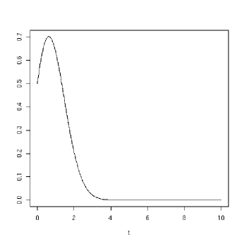
The last inquality follows by Figure 5 and by noting that $(1-\Phi(t))(t+1)^{2}$ is continuous, unimodal, and bounded by 1.

Figure 5: Plot of $(1-\Phi(t))(t+1)^{2}$.

Therefore

$$\sup_{\beta\in\mathcal{B}}\mathbb{P}(A_{j}^{c})|\beta_{j}|^{2}=\max\{\tau_{n}^{2},\lambda_{\text{max}}^{2}\}$$ (35)

Hence, it is sufficient to choose $\tau_{nj}^{2}=2s_{nj}^{2}$ and to note that

$$\lambda_{\text{max}}^{2}\asymp s_{nj}^{2}\asymp\varepsilon^{2}/\Delta_{nj}.$$

This implies

$$\sup_{\beta\in\mathcal{B}}\mathbb{P}(A_{j}^{c})|\beta_{j}|^{2}=O(s_{nj}^{2}).$$ (36)

As we are summing over $j$ in the risk, we conclude that

$$\limsup_{n\rightarrow\infty}\sup_{\beta\in\mathcal{B}}\,\gamma_{n}^{-1}R(\hat{\beta}_{n},\beta)<\infty$$

where

$$\gamma_{n}=\max_{j}\frac{\varepsilon^{2}}{\Delta_{nj}}.$$

Proof B.16 (Proof of Theorem 6).

We use the same notations and conventions as in the proof of Theorem 2.3. Note that if we define $\sigma_{nj}^{2}=\varepsilon^{2}/\Delta_{nj}$, then the linear oracle risk is

$$R(\beta_{*},\beta)=\min_{\tilde{\beta}=\boldsymbol{\lambda}(\mathbf{B}_{n})}R(\tilde{\beta},\beta)=\sum_{j=1}^{p}\frac{|\beta_{j}|^{2}\sigma_{nj}^{2}}{\sigma_{nj}^{2}+|\beta_{j}|^{2}}=\sum_{j=1}^{p}\frac{|\beta_{j}|^{2}s_{nj}^{2}}{s_{nj}^{2}+\Omega_{n}^{2}|\beta_{j}|^{2}}.$$ (37)

we bound the $j^{th}$ term in the loss:

$$|\hat{\beta}_{j}-\beta|^{2}$$

$$=\mathbf{1}_{A_{j}}\left[|Z_{nj}|^{2}-\frac{\overline{Z_{nj}}s_{nj}^{2}(\beta_{j}+Z_{nj})}{|\beta_{j}+Z_{nj}|^{2}}-\frac{Z_{nj}s_{nj}^{2}\overline{(\beta_{j}+Z_{nj})}}{|\beta_{j}+Z_{nj}|^{2}}+\frac{s_{nj}^{4}}{|\beta_{j}+Z_{nj}|^{2}}\right]+$$

$$\qquad\qquad+\mathbf{1}_{A_{j}^{c}}|\beta_{j}|^{2}$$

$$=\mathbf{1}_{A_{j}}\left[|Z_{nj}|^{2}-\frac{|Z_{nj}|^{2}s_{nj}^{2}}{|\beta_{j}+Z_{nj}|^{2}}-\frac{s_{nj}^{2}(|Z_{nj}|^{2}+\beta_{j}\overline{Z_{nj}}+\overline{\beta_{j}}Z_{nj})}{|\beta_{j}+Z_{nj}|^{2}}+\frac{s_{nj}^{4}}{|\beta_{j}+Z_{nj}|^{2}}\right]+$$

$$\qquad\qquad+\mathbf{1}_{A_{j}^{c}}|\beta_{j}|^{2}$$

$$=\mathbf{1}_{A_{j}}\left[|Z_{nj}|^{2}-\left(\frac{s_{nj}^{2}(|\beta_{j}+Z_{nj}|^{2}-|\beta_{j}|^{2})}{|\beta_{j}+Z_{nj}|^{2}}\right)+\frac{s_{nj}^{4}}{|\beta_{j}+Z_{nj}|^{2}}\right]+\mathbf{1}_{A_{j}^{c}}|\beta_{j}|^{2}$$

$$=\mathbf{1}_{A_{j}}\left[|Z_{nj}|^{2}-s_{nj}^{2}+\left(\frac{s_{nj}^{2}|\beta_{j}|^{2}}{|\beta_{j}+Z_{nj}|^{2}}\right)+\frac{s_{nj}^{4}}{|\beta_{j}+Z_{nj}|^{2}}\right]+\mathbf{1}_{A_{j}^{c}}|\beta_{j}|^{2}$$

$$\leq|Z_{nj}|^{2}+\mathbf{1}_{A_{j}}\left(\frac{s_{nj}^{2}|\beta_{j}|^{2}}{|\beta_{j}+Z_{nj}|^{2}}\right)+\mathbf{1}_{A_{j}^{c}}|\beta_{j}|^{2}.$$

$$=|Z_{nj}|^{2}+\mathbf{1}_{A_{j}}\left(\frac{s_{nj}^{2}|\beta_{j}|^{2}}{s_{nj}^{2}+\Omega_{n}^{2}|\beta_{j}|^{2}}\right)\left(\frac{s_{nj}^{2}+\Omega_{n}^{2}|\beta_{j}|^{2}}{|\beta_{j}+Z_{nj}|^{2}}\right)+\mathbf{1}_{A_{j}^{c}}|\beta_{j}|^{2}.$$

By the previous proof, we see that the expected value of the first and third term go to zero uniformly over $\beta\in\mathcal{B}$ at rate $O(1/\Delta_{nj})$; the same rate as the oracle. For the second term, notice that

$$\mathbf{1}_{A_{j}}\left(\frac{s_{nj}^{2}+\Omega_{n}^{2}|\beta_{j}|^{2}}{|\beta_{j}+Z_{nj}|^{2}}\right)\leq\mathbf{1}_{A_{j}}\left(1+\frac{\Omega_{n}^{2}|\beta_{j}|^{2}}{|\beta_{j}+Z_{nj}|^{2}}\right)\lesssim\frac{\mathbf{1}_{A_{j}}|\beta_{j}|^{2}}{|\beta_{j}+Z_{nj}|^{2}}=:G_{nj}$$

for $n$ large enough, by assumption (A5). Then our goal is to show that

$$\limsup_{n\rightarrow\infty}\sup_{\beta\in\mathcal{B}}\mathbb{E}G_{nj}<\infty.$$

First, due to $G_{nj}$ being rotationally symmetric (once we use $|||\cdot|||$ instead of $|\cdot|$), we renormalize to transform $Z_{nj}$ into a vector $\tilde{Z}$ with independent standard normal components

$$G_{nj} =\mathbf{1}_{A_{j}}\left(\frac{|||\beta_{j}|||^{2}}{|||\beta_{j}+Z_{nj}|||^{2}}\right)$$

$$=\mathbf{1}_{\tilde{A}_{j}}\left(\frac{|||U^{\top}\beta_{j}|||^{2}}{|||U^{\top}\beta_{j}+U^{\top}Z_{nj}|||^{2}}\right)$$

$$=\mathbf{1}_{\tilde{A}_{j}}\left(\frac{|||\tilde{\beta}_{j}|||^{2}}{|||\tilde{\beta}_{j}+\Lambda_{nj}^{1/2}\tilde{Z}|||^{2}}\right).$$

We define $\Lambda_{nj}$ and $U$ in the previous proof and $\tilde{A}_{j}:=\{||\tilde{\beta}_{j}+\Lambda_{nj}^{1/2}\tilde{Z}||^{2}>s_{nj}^{2}$.

We break bounding $\mathbb{E}G_{nj}$ into cases.

Case 1: $|||\tilde{\beta}_{j}|||^{2}\leq s_{nj}^{2}$
We see from the definition of $\mathbf{1}_{\tilde{A}_{j}}$

$$G_{nj}\leq\mathbf{1}_{\tilde{A}_{j}}\left(\frac{s_{nj}^{2}}{|||\tilde{\beta}+\Lambda_{nj}\tilde{Z}|||^{2}}\right)<\mathbf{1}_{\tilde{A}_{j}}\left(\frac{s_{nj}^{2}}{s_{nj}^{2}}\right)\leq 1$$ (38)

Case 2: $|||\tilde{\beta}|||^{2}>s_{nj}^{2}$
Note that by the nonnegativity of $G_{nj}$

$$\mathbb{E}G_{nj}=\int_{0}^{\infty}\mathbb{P}(G_{nj}>\tau)\,d\tau.$$

As an aside, the random variables considered don’t put any positive mass at any points, so we don’t need to worry about whether the boundaries of integration are included. For $\tau>0$,

$$\mathbb{P}(G_{nj}>\tau) =\mathbb{P}\left(s_{nj}^{2}\leq|||\tilde{\beta}+\Lambda_{nj}^{1/2}\tilde{Z}|||^{2}<\frac{|||\tilde{\beta}|||^{2}}{\tau}\right)$$

$$=\begin{cases}0&\tau\geq\frac{|||\tilde{\beta}|||^{2}}{s_{nj}^{2}}\\ \mathbb{P}\left(s_{nj}^{2}\leq|||\tilde{\beta}+\Lambda_{nj}^{1/2}\tilde{Z}|||^{2}<\frac{|||\tilde{\beta}|||^{2}}{\tau}\right)&\text{o.w.}\end{cases}$$

Therefore, for any $c^{2}>0$,

$$\mathbb{E}G_{nj} =\int_{0}^{\infty}\mathbb{P}(G_{nj}>\tau)\,d\tau$$

$$=\int_{0}^{c^{2}}\mathbb{P}(G_{nj}>\tau)\,d\tau+\int_{c^{2}}^{\frac{|||\tilde{\beta}|||^{2}}{s_{nj}^{2}}}\mathbb{P}(G_{nj}>\tau)\,d\tau$$

$$\leq c^{2}+\left(\frac{|||\tilde{\beta}|||^{2}}{s_{nj}^{2}}\right)\mathbb{P}(G_{nj}>c^{2})$$

$$\leq c^{2}+\left(\frac{|||\tilde{\beta}|||^{2}}{s_{nj}^{2}}\right)\mathbb{P}\left(|||\tilde{\beta}+\Lambda_{nj}^{1/2}\tilde{Z}|||^{2}<\frac{|||\tilde{\beta}|||^{2}}{c^{2}}\right)$$

If $c^{2}>1$, then the mean of of the random variable $\tilde{\beta}+\Lambda_{nj}^{1/2}\tilde{Z}$ will be outside of the circle centered at zero with radius $||\tilde{\beta}||/c$. Hence, by Lemma 29 if we define $\lambda_{\text{max}}^{2}:=\max\{\text{diag}(\Lambda_{nj})\}$, then it follows that

$$\mathbb{P}\left(|||\tilde{\beta}+\Lambda_{nj}^{1/2}\tilde{Z}|||^{2}<\frac{|||\tilde{\beta}|||^{2}}{c^{2}}\right)\leq\mathbb{P}\left(|||\tilde{\beta}+\lambda_{\text{max}}\tilde{Z}|||^{2}<\frac{|||\tilde{\beta}|||^{2}}{c^{2}}\right).$$ (39)

Using this, observe

$$\left(\frac{|||\tilde{\beta}|||^{2}}{s_{nj}^{2}}\right)\mathbb{P}\left(|||\tilde{\beta}+\Lambda_{nj}^{1/2}\tilde{Z}|||^{2}<\frac{|||\tilde{\beta}|||^{2}}{c^{2}}\right)$$

$$\leq\left(\frac{|||\tilde{\beta}|||^{2}}{s_{nj}^{2}}\right)\mathbb{P}\left(|||\tilde{\beta}/\lambda_{\text{max}}+\tilde{Z}|||^{2}<\frac{|||\tilde{\beta}/\lambda_{\text{max}}|||^{2}}{c^{2}}\right)$$

$$\leq\left(\frac{|||\tilde{\beta}|||^{2}}{s_{nj}^{2}}\right)\left(1-\Phi\left(\left(1-\frac{1}{c}\right)|||\tilde{\beta}/\lambda_{\text{max}}|||\right)\right)$$

$$=\left(\frac{|||\tilde{\beta}|||^{2}}{s_{nj}^{2}}\right)\left(1-\Phi\left(\left(1-\frac{1}{c}\right)|||\tilde{\beta}/\lambda_{\text{max}}|||\right)\right)$$

$$=\left(\frac{(\lambda_{\text{max}}t)^{2}}{s_{nj}^{2}}\right)\left(1-\Phi\left(\left(1-\frac{1}{c}\right)t\right)\right)$$

$$=\left(\frac{\lambda_{\text{max}}^{2}}{s_{nj}^{2}}\right)\left[t^{2}\left(1-\Phi\left(\left(1-\frac{1}{c}\right)t\right)\right)\right]$$

Where we have transformed $t=|||\tilde{\beta}|||/\lambda_{\text{max}}$. Hence, as $s_{nj}^{2}\asymp\lambda_{\text{max}}^{2}$ and

$$\sup_{\frac{s_{nj}}{\lambda_{\text{max}}}\leq t\leq\frac{T}{\lambda_{\text{max}}}}t^{2}\left(1-\Phi\left(\left(1-\frac{1}{c}\right)t\right)\right)\leq\sup_{0\leq t\leq\infty}t^{2}\left(1-\Phi\left(\left(1-\frac{1}{c}\right)t\right)\right)\leq 1$$

we see that

$$\left(\frac{|||\tilde{\beta}|||^{2}}{s_{nj}^{2}}\right)\mathbb{P}\left(|||\tilde{\beta}+\Lambda_{nj}^{1/2}\tilde{Z}|||^{2}<\frac{|||\tilde{\beta}|||^{2}}{c^{2}}\right)=O(1),$$

independent of $\beta$. And we conclude that

$$\mathbb{E}G_{nj}=O(1),$$

again, independent of $\beta$. This ends the proof.

Proof B.17 (Proof of Theorem 7).

Observe

$$\lim_{n\rightarrow\infty}\sup_{\beta\in\mathcal{B}}\mathbb{E}_{(D_{i}),X_{n}}||\hat{\beta}-\beta||^{2} =\lim_{n\rightarrow\infty}\sup_{\beta\in\mathcal{B}}\mathbb{E}_{(D_{i})}\mathbb{E}_{X_{n}|(D_{i})}||\hat{\beta}-\beta||^{2}$$

$$\leq\lim_{n\rightarrow\infty}\mathbb{E}_{(D_{i})}\sup_{\beta\in\mathcal{B}}R(\hat{\beta},\beta).$$ (40)

Therefore it suffices to exchange the limit and integral. To accomplish this we appeal to the following bound from (32). Define $f_{n}:=\sup_{\beta\in\mathcal{B}}\mathbb{E}_{X_{n}|(D_{i})}||\hat{\beta}-\beta||^{2}$. Then

$$|f_{n}| :=\sum_{j=1}^{p}f_{j}$$

$$=\sum_{j=1}^{p}|\hat{\beta}_{j}-\beta_{j}|^{2}$$

$$\leq\sup_{\beta\in\mathcal{B}}\mathbb{E}_{X_{n}|(D_{i})}\sum_{j=1}^{p}\left[\mathbf{1}_{A_{j}}\left(|Z_{nj}|+s_{nj}\right)^{2}+\mathbf{1}_{A_{j}^{c}}|\beta_{j}|^{2}\right]$$

$$\leq\sum_{j=1}^{p}\left(\frac{\varepsilon^{2}}{\Delta_{nj}}+2s_{nj}\sqrt{\frac{\varepsilon^{2}}{\Delta_{nj}}}+s_{nj}^{2}+T^{2}\right)$$

$$\leq\sum_{j=1}^{p}\left(\frac{\varepsilon^{2}}{\Delta_{nj}}\left(1+2\Omega_{n}^{2}+(\Omega_{n}^{2})^{2}\right)+T^{2}\right)$$

$$=\sum_{j=1}^{p}\left(\frac{\varepsilon^{2}}{\Delta_{nj}}(\Omega_{n}^{2}+1)^{2}+T^{2}\right) =:\sum_{j=1}^{p}g_{j} =:g_{n}.$$

Therefore, if we can exchange the limit and integral, then by the previous two proofs we can conclude that the limit is zero. We appeal to the following. We say a set of random variables $\{X_{t}:t\in\mathcal{T}\}$ is uniformly integrable if

$$\lim_{x\rightarrow\infty}\sup_{t\in\mathcal{T}}\mathbb{E}|X_{t}|\mathbf{1}_{|X_{t}|>x}=0.$$

It holds that if $X_{t}\rightarrow X$ with probability one and $\{X_{t}:t\in\mathcal{T}\}$ is uniformly integrable, then $\mathbb{E}X_{t}\rightarrow\mathbb{E}X$. Hence, we wish to show that $f_{n}$ is uniformly integrable. It holds that if each term in the sum over $j$ is uniformly integrable, then $f_{n}$ is uniformly integrable as well.

Note that

$$\mathbb{E}|f_{j}|\mathbf{1}_{|f_{j}|>x} =x\mathbb{P}(f_{j}>x)+\int_{x}^{\infty}\mathbb{P}(f_{j}>y)dy$$

$$\leq x\mathbb{P}(g_{j}>x)+\int_{x}^{\infty}\mathbb{P}(g_{j}>y)dy$$

For large $x$, $x>T^{2}$ and for large $n$, $\Omega_{n}\asymp 1$. Therefore, we only need deal with the term $\epsilon^{2}/\Delta_{nj}$.

Using assumption (B4), continuing the above with relevant terms, and noticing that $\sup_{n}f_{n}$ occurs at $n=1$, it follows that for $x$ large enough

$$x\mathbb{P}\left(\frac{1}{|D_{1j}|^{2}}>x\right)+\int_{x}^{\infty}\left(\frac{1}{|D_{1j}|^{2}}>y\right)dy =x\left(\frac{1}{x^{\rho}}\right)+\int_{x}^{\infty}\left(\frac{1}{y^{\rho}}\right)dy$$

$$=\left(\frac{1}{x^{\rho-1}}\right)+\int_{x}^{\infty}\left(\frac{1}{y^{\rho}}\right)dy$$

$$\rightarrow 0.$$

This allows for the exchange of integration end hence shows the desired result.

Proof B.18 (Proof of Proposition 13).

We can expand (11) for any $\boldsymbol{\lambda}(\mathbf{B}_{n})\in\mathcal{E}$ as

$$R(\boldsymbol{\lambda}):=R_{\beta}(\boldsymbol{\lambda}(\mathbf{B}_{n}))=\sum_{j=1}^{p}\left[(\lambda_{j}-1)^{2}|\beta_{j}|^{2}+\frac{\varepsilon^{2}\lambda_{j}^{2}}{\Delta_{nj}}\right].$$ (41)

To form an estimator of $R$, we notice that $\mathbb{E}_{\beta_{j}}(|B_{nj}|^{2}-\varepsilon^{2}/\Delta_{nj})=|\beta_{j}|^{2}$. Hence,

$$\hat{R}(\boldsymbol{\lambda}):=\sum_{j=1}^{p}\left[(\lambda_{j}-1)^{2}\left(|B_{nj}|^{2}-\frac{\varepsilon^{2}}{\Delta_{nj}}\right)+\frac{\varepsilon^{2}\lambda_{j}^{2}}{\Delta_{nj}}\right]$$ (42)

is an unbiased estimate of $R(\boldsymbol{\lambda})$. We can make a substitution

$$\hat{\psi}_{j}:=(|B_{nj}|^{2}-\varepsilon^{2}/\Delta_{nj})/|B_{nj}|^{2},$$

which produces

$$\hat{R}(\boldsymbol{\lambda})=\sum_{j=1}^{p}\left[(\lambda_{j}-\hat{\psi}_{j})^{2}|B_{nj}|^{2}\right]+\varepsilon^{2}\sum_{j=1}^{p}\left(\frac{\hat{\psi}_{j}}{\Delta_{nj}}\right).$$ (43)

Finally, note that the second term in $\hat{R}$ doesn’t depend on $\boldsymbol{\lambda}$, so it can be ignored for minimization purposes. Define

$$\hat{R}_{n}(\boldsymbol{\lambda}):=\sum_{j=1}^{p}(\lambda_{j}-\hat{\psi}_{j})^{2}|B_{nj}|^{2}$$ (44)

which is proportional to $\hat{R}(\boldsymbol{\lambda})$. This is our objective function for formulating estimators.

However, there are some natural restrictions. First, define $\mathcal{L}:=[0,1]^{p}$. If we consider a transformed version of (41) by making the substitution $\psi_{j}:=|\beta_{j}|^{2}/(|\beta_{j}|^{2}+\Delta_{nj})$, then

$$R(\boldsymbol{\lambda})=\sum_{j=1}^{p}\left[(\lambda_{j}-\psi_{j})^{2}\left(|\beta_{j}|^{2}+\frac{\varepsilon^{2}}{\Delta_{nj}}\right)+\varepsilon^{2}\left(\frac{\psi_{j}}{\Delta_{nj}}\right)\right].$$ (45)

By inspection, the minimizer of (45) falls in $\mathcal{L}$ as $\psi_{j}\in[0,1]$ for each $j$. Hence, we cannot get a lower risk by considering any more general sets and thus confine our attention to $\boldsymbol{\lambda}\in\mathcal{L}$.

Proof B.19 (Proof of Theorem 3.10).

Direct computation shows that

$$R_{1}=\min_{\lambda}\sum_{j=1}^{p}(1-\lambda_{j})^{2}|B_{j}|^{2}+\varepsilon^{2}\sum_{j=1}^{p}\frac{\lambda_{j}^{2}}{\Delta_{nj}}$$

and

$$R_{2}=\min_{\lambda}\sum_{j=1}^{p}(1-\lambda_{j})^{2}|B_{j}|^{2}+\frac{\varepsilon^{2}}{n}\sum_{j=1}^{p}\frac{\lambda_{j}^{2}}{|D_{n}|_{j}^{2}}.$$

This implies that

$$R_{1}=\sum_{j=1}^{p}\frac{\frac{\varepsilon^{2}}{\Delta_{nj}}|\beta_{j}|^{2}}{|\beta_{j}|^{2}+\frac{\varepsilon^{2}}{\Delta_{nj}}}=\sum_{j=1}^{p}\frac{|\beta_{j}|^{2}}{\frac{\Delta_{nj}}{\varepsilon^{2}}|\beta_{j}|^{2}+1}$$

and

$$R_{2}=\sum_{j=1}^{p}\frac{\frac{\varepsilon^{2}}{n|D_{n}|_{j}^{2}}|\beta_{j}|^{2}}{|\beta_{j}|^{2}+\frac{\varepsilon^{2}}{n|D_{n}|_{j}^{2}}}=\sum_{j=1}^{p}\frac{|\beta_{j}|^{2}}{\frac{n|D_{n}|_{j}^{2}}{\varepsilon^{2}}|\beta_{j}|^{2}+1}.$$

Hence, the results reduces to comparing $\Delta_{nj}$ to $n|D_{n}|_{j}^{2}$. Note

$$|D_{n}|^{2}=D_{n}^{*}D_{n}=\frac{1}{n^{2}}\sum_{i,q}D_{i}^{*}D_{q}$$

therefore

$$n|D_{n}|_{j}^{2}=\frac{1}{n}\sum_{i,q}D_{ij}^{*}D_{qj}.$$

Observe

$$n|D_{n}|_{j}^{2}-\Delta_{nj}= \frac{1}{n}\sum_{i,q}D_{ij}^{*}D_{qj}-\sum_{i=1}^{n}|D_{ij}|^{2}$$

$$= \left(\frac{1}{n}-1\right)\Delta_{nj}+\sum_{i\neq q}D_{ij}^{*}D_{qj}$$

$$\leq \frac{1}{n}\left(-(n-1)\Delta_{nj}+\sum_{i\neq q}D_{ij}^{*}D_{qj}\right)$$

$$\lesssim -\left(n-1\right)\sum_{i=1}^{n}|D_{ij}|^{2}+\sum_{i\neq q}D_{ij}^{*}D_{qj}$$

$$\leq -\left(n-1\right)\sum_{i=1}^{n}|D_{ij}|^{2}+\sum_{i\neq q}(|D_{ij}|^{2}+|D_{qj}|^{2})/2$$

$$= -\left(n-1\right)\sum_{i=1}^{n}|D_{ij}|^{2}+(n-1)\sum_{i=1}^{n}|D_{ij}|^{2}=0$$

where the last inequality follows as $|D_{ij}||D_{iq}|\leq(|D_{ij}|^{2}+|D_{qj}|^{2})/2$ by the arithmetic geometric inequality.

References

- Bahadur (1954) {barticle}[author] \bauthor\bsnmBahadur, \bfnmR. R.\binitsR. R. (\byear1954). \btitleSufficiency and statistical decision functions. \bjournalThe Annals of Mathematical Statistics \bvolume25 \bpages423–462. \endbibitem
- Beran (2000) {barticle}[author] \bauthor\bsnmBeran, \bfnmR.\binitsR. (\byear2000). \btitleScatterplot smoothers: superefficiency through basis economy. \bjournalJournal of the American Statistical Association \bvolume95 \bpages155–171. \endbibitem
- Berenstein and Patrick (1990) {barticle}[author] \bauthor\bsnmBerenstein, \bfnmCarlos\binitsC. and \bauthor\bsnmPatrick, \bfnmE. Vincent\binitsE. V. (\byear1990). \btitleExact deconvolution for multiple convolution operators - an overview, plus performance characterizations for imaging sensors. \bjournalProceedings of the IEEE \bvolume78 \bpages723–734. \endbibitem
- Bertero and Boccacci (1998) {bbook}[author] \bauthor\bsnmBertero, \bfnmM.\binitsM. and \bauthor\bsnmBoccacci, \bfnmP.\binitsP. (\byear1998). \btitleIntroduction to inverse problems in imaging. \bpublisherIOP Publishing, \baddressBristol. \endbibitem
- Brown (1975) {barticle}[author] \bauthor\bsnmBrown, \bfnmLawrence D.\binitsL. D. (\byear1975). \btitleEstimation with incompletely specified loss functions (the case of several location parameters. \bjournalJournal of the American Statistical Association \bvolume70 \bpages417–427. \endbibitem
- Brown, Nie and Xie (2011) {barticle}[author] \bauthor\bsnmBrown, \bfnmLawrence D.\binitsL. D., \bauthor\bsnmNie, \bfnmHui\binitsH. and \bauthor\bsnmXie, \bfnmXianchao\binitsX. (\byear2011). \btitleEnsemble minimax estimation for multivariate normal means. \bjournalThe Annals of Statistics. \endbibitem
- Candés and Donoho (2002) {barticle}[author] \bauthor\bsnmCandés, \bfnmEmmanuel J.\binitsE. J. and \bauthor\bsnmDonoho, \bfnmDavid L.\binitsD. L. (\byear2002). \btitleRecovering edges in ill-posed inverse problems: optimality if curvelet frames. \bjournalAnnals of Statistics \bvolume30 \bpages784–842. \endbibitem
- Casey and Walnut (1994) {barticle}[author] \bauthor\bsnmCasey, \bfnmStephen\binitsS. and \bauthor\bsnmWalnut, \bfnmDavid\binitsD. (\byear1994). \btitleSystems of convolution equations, deconvolutions, shannon sampling, and the wavelet and Gabor transforms. \bjournalSIAM Review \bvolume36 \bpages537–577. \endbibitem
- Cavalier (2008) {barticle}[author] \bauthor\bsnmCavalier, \bfnmL.\binitsL. (\byear2008). \btitleNonparametric statistical inverse problems. \bjournalInverse Problems \bvolume24. \endbibitem
- Cavalier and Tsybakov (2002) {barticle}[author] \bauthor\bsnmCavalier, \bfnmLaurent\binitsL. and \bauthor\bsnmTsybakov, \bfnmA. B.\binitsA. B. (\byear2002). \btitleSharp adaptation for inverse problems with random noise. \bjournalProbability Theory and Related Fields \bvolume123 \bpages323–354. \endbibitem
- Cavalier et al. (2002) {barticle}[author] \bauthor\bsnmCavalier, \bfnmL.\binitsL., \bauthor\bsnmGolubev, \bfnmG. K.\binitsG. K., \bauthor\bsnmPicard, \bfnmD.\binitsD. and \bauthor\bsnmTsybakov, \bfnmA. B.\binitsA. B. (\byear2002). \btitleOracle inequlities for inverse problems. \bjournalAnnals of Statistics \bvolume30 \bpages843–874. \endbibitem
- Correia et al. (2002) {barticle}[author] \bauthor\bsnmCorreia, \bfnmS.\binitsS., \bauthor\bsnmCarbillet, \bfnmM.\binitsM., \bauthor\bsnmBoccacci, \bfnmP.\binitsP., \bauthor\bsnmBertero, \bfnmM.\binitsM. and \bauthor\bsnmFini, \bfnmL.\binitsL. (\byear2002). \btitleRestoration of interferometric images. \bjournalAstronomy & Astropysics \bvolume387 \bpages733–743. \endbibitem
- Donoho (1995) {barticle}[author] \bauthor\bsnmDonoho, \bfnmDavid L.\binitsD. L. (\byear1995). \btitleNonlinear solution of linear inverse problems by wavelet-vaguelette decomposition. \bjournalApplied and Computational Harmonic Analysis \bpages101–126. \endbibitem
- Donoho and Johnstone (1995) {barticle}[author] \bauthor\bsnmDonoho, \bfnmDavid L.\binitsD. L. and \bauthor\bsnmJohnstone, \bfnmIain M.\binitsI. M. (\byear1995). \btitleAdapting to Unknown Smoothness via Wavelet Shrinkage. \bjournalJournal of the American Statistical Association \bvolume90 \bpages1200–1224. \endbibitem
- Gray (2001) {bbook}[author] \bauthor\bsnmGray, \bfnmRobert M.\binitsR. M. (\byear2001). \btitleToeplitz and circulant matrices: a review. \endbibitem
- Halko, Martinsson and Tropp (2009) {barticle}[author] \bauthor\bsnmHalko, \bfnmNick\binitsN., \bauthor\bsnmMartinsson, \bfnmPer Gunnar\binitsP. G. and \bauthor\bsnmTropp, \bfnmJoel A\binitsJ. A. (\byear2009). \btitleFinding structure with randomness: Stochastic algorithms for constructing approximate matrix decompositions. \bjournalCalifornia Inst. Tech., Sep. 2009 \bvolumeACM Report 2009-05. \endbibitem
- Horn and Johnson (1985) {bbook}[author] \bauthor\bsnmHorn, \bfnmRoger A.\binitsR. A. and \bauthor\bsnmJohnson, \bfnmCharles R.\binitsC. R. (\byear1985). \btitleMatrix Analysis. \bpublisherCambridge University Press. \endbibitem
- Mallet (2009) {bbook}[author] \bauthor\bsnmMallet, \bfnmStephane\binitsS. (\byear2009). \btitleA wavelet tour of signal processing: the sparse way, \beditionThird ed. \bpublisherElsevier, \baddressOxford, UK. \endbibitem
- Ólafsson and Quinto (2005) {bbook}[author] \bauthor\bsnmÓlafsson, \bfnmGestur\binitsG. and \bauthor\bsnmQuinto, \bfnmEric Todd\binitsE. T. (\byear2005). \btitleThe Radon transform, inverse problems, and tomography: Short Course. \bpublisherAmerican Mathematical Society, \baddressAtlanta Georgia. \endbibitem
- O’Sullivan (1986) {barticle}[author] \bauthor\bsnmO’Sullivan, \bfnmFinbarr\binitsF. (\byear1986). \btitleA statistical perspective on ill-posed inverse problems. \bjournalStatistical Science \bvolume1 \bpages502–527. \endbibitem
- Piana and Bertero (1996) {barticle}[author] \bauthor\bsnmPiana, \bfnmM.\binitsM. and \bauthor\bsnmBertero, \bfnmM.\binitsM. (\byear1996). \btitleRegularized deconvolution of multiple images of the same object. \bjournalJ. Opt. Soc. Am. A \bvolume13 \bpages1516–1523. \endbibitem
- Robertson, Wright and Dykstra (1988) {bbook}[author] \bauthor\bsnmRobertson, \bfnmTim\binitsT., \bauthor\bsnmWright, \bfnmF. T.\binitsF. T. and \bauthor\bsnmDykstra, \bfnmR. L.\binitsR. L. (\byear1988). \btitleOrder Restricted Statistical Inference. \bpublisherJohn Wiley and Sons, \baddressGreat Britain. \endbibitem
- Starck, Pantin and Murtagh (2002) {barticle}[author] \bauthor\bsnmStarck, \bfnmJ. L.\binitsJ. L., \bauthor\bsnmPantin, \bfnmE.\binitsE. and \bauthor\bsnmMurtagh, \bfnmF.\binitsF. (\byear2002). \btitleDeconvolution in Astronomy: a review. \bjournalPublications of the Astronomy Society of the Pacific \bvolume114 \bpages1051-1069. \endbibitem
- Stein (1981) {barticle}[author] \bauthor\bsnmStein, \bfnmC. M.\binitsC. M. (\byear1981). \btitleEstimation of the mean of a multivariate normal distribution. \bjournalThe Annals of Statistics \bvolume90 \bpages1247–1256. \endbibitem
- Tenorio (2001) {barticle}[author] \bauthor\bsnmTenorio, \bfnmLuis\binitsL. (\byear2001). \btitleStatistical regularization of inverse problems. \bjournalSIAM Review \bvolume43 \bpages347–366. \endbibitem
- van Dyk et al. (2006) {barticle}[author] \bauthor\bparticlevan \bsnmDyk, \bfnmDavid\binitsD., \bauthor\bsnmConnors, \bfnmAlanna\binitsA., \bauthor\bsnmEsch, \bfnmDavid N.\binitsD. N., \bauthor\bsnmFreeman, \bfnmPeter\binitsP., \bauthor\bsnmKang, \bfnmHosung\binitsH., \bauthor\bsnmKarovska, \bfnmMargarita\binitsM., \bauthor\bsnmKashyap, \bfnmVinay\binitsV., \bauthor\bsnmSiemiginowska, \bfnmAneta\binitsA. and \bauthor\bsnmZezas, \bfnmAndreas\binitsA. (\byear2006). \btitleDeconvolution in high-energy Astrophysics: science, instrumentation, and methods. \bjournalBayesian Analysis \bvolume1 \bpages189-236. \endbibitem
- Wahba (1990) {bbook}[author] \bauthor\bsnmWahba, \bfnmGrace\binitsG. (\byear1990). \btitleSpline Models for Observational Data. \bpublisherSIAM, \baddressPhiladelphia, PA. \endbibitem