MEKS: a program for computation
of inclusive jet cross sections at hadron colliders
Abstract
EKS is a numerical program that predicts differential cross sections for production of single-inclusive hadronic jets and jet pairs at next-to-leading order (NLO) accuracy in a perturbative QCD calculation. We describe MEKS 1.0, an upgraded EKS program with increased numerical precision, suitable for comparisons to the latest experimental data from the Large Hadron Collider and Tevatron. The program integrates the regularized patron-level matrix elements over the kinematical phase space for production of two and three partons using the VEGAS algorithm. It stores the generated weighted events in finely binned two-dimensional histograms for fast offline analysis. A user interface allows one to customize computation of inclusive jet observables. Results of a benchmark comparison of the MEKS program and the commonly used FastNLO program are also documented.
keywords:
Inclusive jet production; perturbative quantum chromodynamics; hadron colliderPROGRAM SUMMARY
Manuscript Title: MEKS 1.0: a program for computation
of inclusive jet cross sections at hadron colliders
Authors: Jun Gao, Zhihua Liang, Davison E. Soper, Hung-Liang
Lai, Pavel M. Nadolsky, C.-P. Yuan
Program Title: MEKS 1.0
Journal Reference:
Catalogue identifier:
Preprint number:
SMU-HEP-12-10
Licensing provisions: none
Programming language: Fortran (main program), C (CUBA
library and analysis program).
Computer: all
Operating system: any UNIX-like system
RAM: 300 MB
Supplementary material:
Keywords: Inclusive jet production; perturbative quantum
chromodynamics; hadron collider
Classification: 11.1
Nature of problem: Computation of differential cross sections
for inclusive production of single hadronic jets and jet pairs at
next-to-leading order accuracy in perturbative quantum chromodynamics.
Solution method: Upon subtraction of infrared singularities,
the hard-scattering matrix elements are integrated over available
phase space using an optimized VEGAS algorithm. Weighted events are
generated and filled into a finely binned two-dimensional histogram,
from which the final cross sections with typical experimental binning
and cuts are computed by an independent analysis program. Monte Carlo
sampling of event weights is tuned automatically to get better efficiency.
Running time: Depends on details of the calculation and
sought numerical accuracy. See benchmark performance in Section 4.
1 Introduction
Production of particle jets in high-energy collisions is a cornerstone process of the physics program at the CERN Large Hadron Collider (LHC) and Fermilab Tevatron collider. Historically, observation of final-state jets formed by hadrons in collisions confirmed the asymptotic freedom of strong interactions. In modern experiments, measurements of inclusive jet production at and colliders have reached unprecedented precision. They serve both for exacting tests of perturbative quantum chromodynamics (PQCD) and for searches for hypothetical new interactions at the highest energy scales attained. Within PQCD, measurements of single-jet production cross sections at the Tevatron Run-2 constrain the QCD coupling constant [1] and parton distribution functions (PDF) in the proton [2, 3, 4, 5]. Jet production has unique sensitivity to the momentum distribution of gluons with large momentum fractions , which is not available in other scattering processes [6]. Invariant mass distributions of dijets [7], dijet angular distributions [8, 9], and other jet observables at the LHC [10, 11, 12] are examined to search for quark compositeness and heavy particle resonances. All these analyses depend on reliable theoretical computations that continue to evolve to stay on par with experimental developments.
From the experimental point of view, jet production has an advantage of very high statistics and a drawback of sizable systematic errors associated with the complexities of jet reconstruction. On the theory side, predictions for jet observables remain known to next-to-leading order (NLO) only [13, 14, 15, 16]. Theoretical uncertainties due to the QCD scale dependence and the fixed-order model for the jet algorithm are comparable to the experimental errors. Some phenomenological studies also include partial next-to-next-to-leading order contributions to jet cross sections obtained by threshold resummation [17].
This paper describes MEKS, a program for predicting probabilities of observation of a single jet or of jet pairs that are accompanied by arbitrary final states, and . An early numerical code (EKS) for the NLO calculation of single inclusive jet and dijet distributions was developed by S. D. Ellis, Z. Kunszt and D. E. Soper in the 1990’s [13] based on the subtraction method. The MEKS program is based on the original EKS calculation that has been augmented by new elements to boost its stability, flexibility, and efficiency. Two other widely used numerical programs are NLOJET++ [15, 16] – a complete calculation of inclusive one and two jet cross sections at NLO, – and FastNLO [18, 19], which provides a fast interpolation of NLOJET++ cross sections in the kinematical bins of already published experimental measurements.111NLOJET++ can also be used to calculate three jet inclusive cross sections, but that feature is not relevant for this paper. Besides these fixed-order calculations, POWHEG combines the NLO jet production cross sections with leading-logarithm QCD showering effects [20].
Precision calculations for these processes are challenging because of the rapid falloff of the cross sections with the jet’s and rapidity. In a typical experimental data set, jet cross sections vary by up to 6-9 orders of magnitude. In addition, large numerical cancelations occur between some and contributions due to the presence of QCD singularities. MEKS undertakes several measures to handle these issues and to achieve relative accuracy of order one percent in the numerical simulations. The MEKS output is produced in the form of two-dimensional differential cross sections (, , …) after integration over the unobserved momentum components using the VEGAS method from the CUBA2.1 library [21]. The Monte-Carlo integration is automatically optimized to improve the speed of the calculation. The generated events are written into finely binned two-dimensional histograms that can be rebinned into any set of coarse bins of a given experiment at the stage of the user’s final analysis. This format is different from the FastNLO format, which provides the cross sections in the coarse bins that are taken from pre-existing experimental publications. Residual theoretical uncertainties in such an NLO calculation are currently comparable to typical experimental errors. Thus, together with the MEKS code, we present a detailed benchmark comparison with the independent FastNLO code and comment on the stability of the NLO jet calculations with respect to the choice of QCD scales.
This document is structured as follows. Section 2 reviews theoretical prerequisites for the calculation of single inclusive jet and dijet cross sections at NLO. Section 3 describes the structure of the program, its inputs and outputs, installation, and running. Section 4 considers the performance of the program and summarizes its benchmark comparison against FastNLO. Section 5 contains the conclusion.
2 Production of hadronic jets at NLO in perturbative QCD
2.1 Factorized cross sections and measurement functions
A jet reveals itself by tracks and calorimeter energy depositions left by final-state hadrons in a collider detector. Numerous particles comprise a typical jet, and their detailed distribution is complicated. Nevertheless the probability for producing the whole jet can be deduced with high confidence from the cross section for production of the partons (quarks or gluons) that are the jet’s progenitors. Each contributing parton-level cross section can be computed in PQCD. It is included into the total cross section for producing the jet according to the jet algorithm, i.e., the convention adopted to define the jet in terms of the four-momenta of its constituent particles. The parton-level prediction must be corrected for effects of final-state showering, hadronization, and event pile-up in order to be compared to the observables recorded by the detector.
PQCD provides a generic cross section for production of partons in scattering of hadrons and with center-of-mass energy ,
| (1) |
Here and are the parton distribution functions (PDFs) of intermediate partons and in the parent nucleons and . The factor is the cross section for hard scattering of and , which is computable as a series in the running coupling strength . The parents’ momentum fractions carried by and are and , while and are the renormalization scale and factorization scale that arise in and the PDFs, respectively.
is the phase space for production of (massless) partons with four-momenta . To relate this parton-level cross section to a jet observable that can be measured, such as the cross section in some experimental bins, it must be folded into an integral
| (2) |
The function represents constraints on the partons’ momenta imposed by various steps of the measurement, including the jet algorithm. The right-hand side of Eq. (2) is summed over all final-state configurations (f.s.c.) and parton types that may contribute. The number of the final states is summed from to infinity, but large- configurations are suppressed by a high power of the small parameter
A next-to-leading-order (NLO) calculation of the single-inclusive jet or dijet cross section includes only and parton scattering contributions. At NLO, the jet observable is represented in the calculation by two functions, and . The expectation of the observable is
| (3) |
The cross sections depend on for the case of two final state partons and on for the case of three final state partons. The parton momenta are determined by the absolute value of the transverse momentum, , the rapidity, , and the azimuthal angle, . Momentum conservation has been applied to reduce the number of independent integration variables. The functions and are symmetric under interchange of the parton labels 1,2,3 and must be related by infrared safety conditions: must approach when the parton momenta and become collinear with each other, or when tends to zero. In Eq. (3), both terms are infrared divergent and need to be regulated by working in space-time dimensions (with ) instead of 4 dimensions.222The needed modifications to the -dimensional integration measure are suppressed in Eq. (3). For this reason, some manipulation is needed to bring into a form in which the integrals can be calculated by Monte Carlo numerical integration.
In this paper, we are concerned with double-differential jet cross sections. That is, there are two variables and that are functions of the parton momenta: and , or and . These functions are infrared-safe in the sense defined above. For instance, might be the invariant mass of the leading two jets in an event, and might be the difference in the rapidities of the two jets, where the jets are defined, for instance, by the jet algorithm. Then the functions in Eq. (3) specify whether the event contributes to a certain bin in a histogram of the cross section:
| (4) |
The subtraction method for calculating is explained in some detail in Ref. [14]. There is no point in repeating this explanation here. It may be helpful, however, to illustrate the final form of the Monte Carlo integration in a simplified model calculation that is independent of rapidities. In the simplified model, we integrate over a single one-dimensional variable in the first term and over two one-dimensional variables and in the second term. After applying the subtraction method to tame divergences, the model integral has the form
| (5) |
There is a divergence from the first term of the second integral arising from the region . However, in this model, the infrared safety property of the jet definition is . Then the divergence is canceled because of the subtraction term. The integral as written is suitable for calculation by Monte Carlo numerical integration.
The program described here is modified from the original EKS program, which used an elaborate method to calculate a double differential jet cross section, because the computer power available when the program was written was quite limited. The method used here is to calculate the jet observables and for each point in the Monte Carlo integration and put them into very small bins. Then a separate analysis routine can calculate the desired cross section in any larger bin desired. In our model calculation, this means that we calculate a collection of integrals
| (6) |
Here the bin widths are very small. From this information, the integral over a larger bin can be calculated later for any and desired. In the program described here, the Monte Carlo points and are chosen using the VEGAS algorithm [22] with some modifications.
2.2 Main theoretical inputs
Theoretical inputs must be selected carefully in the comparisons of NLO cross sections, since they may cause non-negligible differences in predictions.
-
1.
Jet algorithm. When calculating the distribution of jet observables, we need to use the same jet algorithms as the ones in the experimental measurements. In a PQCD calculation, the experimental jet algorithm is approximated by a measurement function that acts on a small number of partons. (See the previous section.) The cone-based Midpoint algorithm [23] is most frequently used at the Tevatron, while the cluster-based anti- algorithm [24] is in standard use at the LHC. The only difference between the Midpoint algorithm and modified Snowmass algorithm [23] used in the original EKS program is that the Midpoint algorithm always uses the midpoint of the two partons’ directions as one of the possible seeds for a new protojet. In the NLO theoretical calculations for single-jet or dijet production that include at most three final-state partons, the cluster-based [25, 26], anti-, and Cambridge-Aachen (CA) [27] algorithms are equivalent. The Midpoint algorithm is generally different from these algorithms.
-
2.
The recombination scheme is a procedure for merging two nearby partons into one jet. For example, the 4D scheme computes the jet’s 4-momentum by adding the 4-momenta of the jet’s constituents. The scheme finds the momentum of the merged jet by adding the scalar values, then averaging over the partons’ directions with the statistical weights given by the individual values [28]. The 4D scheme is often adopted by the recent experiments at both the Tevatron and LHC. Different choices of the recombination scheme can cause differences in the NLO predictions, as will be shown later in the benchmark comparison section. Note that, with the 4D scheme, the jet could be massive, which means that the jet’s pseudorapidity will not be equal to its rapidity.
-
3.
The jet acceptance conditions specify if the jet will be considered in the final observables. For example, to be taken into account, the total transverse momentum of the jet in the acceptance region must be larger than a threshold value of a few tens GeV/c. In NLO calculations of single-inclusive jet distributions, the jet acceptance conditions practically have no effects. In dijet production, they may change the cross sections by small amounts by affecting the selection of two leading jets.
-
4.
Renormalization and factorization scales. The scale choice is only related to theory and has no correspondence in experiment. It is conventional to choose the renormalization and factorization scales to be of the order of the typical transverse momentum of the jet(s): . In contributions with two resolved jets, naturally corresponds to the transverse momentum of either of the final-state jets (which are about equal by momentum conservation). More ambiguity is present in contributions with three resolved jets, when can correspond to the transverse momentum of either of the jets in each event or to a combination of three transverse momenta. The conventional choices made by experimentalists are to set both of the scales to individual jet for single inclusive jet production and to the average of the two leading jets for dijet production.
2.3 Typical kinematical variables
For completeness, we provide definitions of typical kinematical variables arising in recent measurements. The leading jet has the largest transverse momentum among all jets in each scattering event. Single-inclusive jet cross sections may refer either to distributions of the leading jets or individual jets (so that all jets hitting a particular kinematic bin in every event are counted). Currently, MEKS has a built-in mode for computing single-inclusive distributions of individual jets, although distributions for the leading jets can be easily implemented. The transverse momentum and rapidity of the individual jet are denoted by and , respectively.
In dijet production, kinematical variables are formed from the four-momenta of the first and second leading jets, and . Common distributions are given in terms of the dijet’s invariant mass , the maximal absolute rapidity value in the jet pair, and the angular variable .
3 Description of the program
3.1 Algorithm
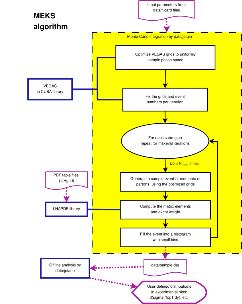
The goal of the MEKS program is to calculate double-differential cross sections for single-inclusive jet or dijet production at hadron colliders up to NLO in QCD. Its basic algorithm is shown in Fig. 1. All executables, input files, and output files are stored in the subdirectory data/. The main computation is carried out in an executable jetbin, which performs Monte-Carlo integration of fully differential NLO cross sections using the VEGAS algorithm provided by the CUBA library [21]. The input parameters are read from several .card files. In view of the rapid falloff of the cross section across the available phase space region, the integration volume is divided into subregions which are handled separately, and additional optimization is performed to achieve percent-level accuracy in each subregion. The integration runs in a sequence of three steps. First, it scans over entire kinematic regions of the jet observables and calculates Monte Carlo sampling weights for different regions in order to improve the efficiency of the sampling. In step 2, the program generates and optimizes the VEGAS grids for MC samplings using the above weights. In the final step, it performs Monte Carlo sampling based on the corresponding VEGAS grids and generates the weighted events. For each sampling event, the program generates independent components of partonic momenta (4 components in subprocesses and 7 components in subprocesses). It then computes the cross section weight for the event as described in Sec. 2, using the parton-level cross sections, PDFs, and measurement functions. Parametrizations of the PDFs are provided by the LHAPDF library [29], which requires PDF table files (.LHgrid) as an input for interpolation. The momentum components and final weight of each event are written into auxiliary two-dimensional histograms in an ASCII file. The bin sizes are chosen to be substantially smaller than in a typical experiment, of order 1 GeV for momentum variables, and 0.1 for rapidity variables. Finally, when the computation is finished, the auxiliary histograms can be rebinned into the bins of a selected experiment using the jetana program.
3.2 Installation
The MEKS code is installed by unpacking the archive (.zip) file and running make in the main directory. An external LHAPDF library is required and the path of the LHAPDF library should be set in the makefile before running make. The compilation requires gcc, g++, and gfortran compilers. The compiler will generate two executables in the subdirectory data: jetbin for generating the intermediate histogram files, and jetana for calculating the final differential cross sections. Running make clean will delete all the compiled libraries and executables.
3.3 The source
The main directory contains 8 source files together with 3 subdirectories. jetbin.f contains the main program for the Monte Carlo sampling. The EKS function RENO() that returns the integral for the jet cross sections is stored in ekscode.f. The module modsub.f contains subroutines for reading the inputs, clustering and selection of jets, recording of the events, generation of the histograms, and interface to the CUBA library. lha_interface.f is the interface to the LHAPDF library. user.inc and var.inc are header files with definitions of variables and common blocks. jetana.cxx is a C++ source file for the offline rebinning of the histogram files into the final double-differential cross sections. These files are not supposed to be changed by the user. Customization of inputs and outputs can be done by editing the module userfunction.f, as described in Sec. 3.6.
Besides the subdirectory data/ described above, the subdirectory lib/ contains a simplified CUBA library. It is written in C and includes only VEGAS algorithm. Examples in the subdirectory example/ show how to set the input files for representative Tevatron and LHC measurements.
3.4 Input parameters
| promode | Observable | Distribution |
|---|---|---|
| 1 | Single-inclusive | |
| 2 | Dijet | |
| 3 | Dijet | |
| 4 | User-specified |
The input parameters are specified in the files with the extension .card. Each line contains a record for one input variable: a character tag with the name of the variable, followed by the variable’s value.
proinput.card specifies overall controls for the computation
-
1.
pdfname is the name of the PDF file to be used in the calculation, e.g., cteq66.LHgrid if CTEQ6.6 central PDFs are used.
-
2.
pdfmem specifies which member of the PDF set from the LHAPDF library is to be invoked. For example, set pdfmem=0 to access the central PDF set or another integer to access an error PDF according to the definition provided by LHAPDF.
-
3.
promode specifies the double-differential distribution. Set promode=1,2, or 3 to produce common distributions listed in Table 1, where the kinematical variables are defined in Sec. 2.3. Alternatively, choose promode=4 to compute a user-defined distribution that is specified in userfunction.f.
-
4.
smode specifies the choice of the hard momentum scale that defines the central value of the factorization and renormalization scales: and , where and are the prefactors of order unity that are input as fscale and rscale later in the card. Currently smode = 1 sets the central scale to the individual jet for single-inclusive jet production and to the average of two leading jets for dijet production. smode = 2 sets the central scales equal to the leading jet’s for both single-inclusive jet and dijet production. For the user-specified calculation mode (promode=4), the central scale should be set directly in userfunction.f by the user.
-
5.
loop specifies the order of the QCD coupling: 0 for a LO calculation and 1 for a full NLO calculation (LO + NLO corrections).
-
6.
ppcollider represents the type of the collider: 0 for a machine and 1 for a machine.
-
7.
sqrtSS gives the center-of-mass energy of the collider in GeV.
-
8.
fscale and rscale are the prefactors for and , cf. the discussion above.
-
9.
iseed specifies the random-number seed used by the VEGAS subroutine. If iseed = 0 (recommended), the seeds are generated randomly from the internal clock readings. The results from different runs will be statistically independent and can be combined to improve the numerical accuracy. Or, the user can specify iseed 0 to reproduce the same pseudorandom numbers in subsequent runs.
-
10.
maxeval specifies the total number of iterations carried out in the calculation as shown in Fig. 1. maxeval controls both the CPU time cost and numerical accuracy of each job. Note that for all the calculation modes except the user-specified one, the numbers () of Monte Carlo sampling points for each iteration and subregion are determined automatically, and are not supposed to be specified by the user. They may differ for different subregions. For example, more sampling points can be placed into a subregion with a large volume or close to the edges of the phase space. Since the offline analysis code can combine results from several independent jobs to improve the numerical accuracy, we suggest that the user runs multiple jobs on a cluster or multi-core machine with maxeval<5, rather than a single job with a large maxeval value.
kininput.card contains parameters for clustering and selection of jets, in the same format as in proinput.card.
-
1.
jetalgo specifies the jet algorithm used in the calculation: 1 for the anti- jet algorithm, 2 for the modified Snowmass algorithm, in which the Midpoint algorithm is a special case of Rsep = 2 at NLO.
-
2.
recscheme sets the recombination scheme used in jet clustering: 1 for the 4D scheme and 2 for the scheme.
-
3.
Rcone sets the cone size or distance parameter for the jet algorithm used.
-
4.
Rsep sets the separation parameter used in the modified Snowmass algorithm. Note that in the theoretical calculations here, the modified Snowmass algorithm with Rsep = 2 is equivalent to the Midpoint algorithm.
-
5.
ptcut and ycut specify conditions for jet acceptance, i.e., the lowest value of and largest absolute value of the rapidity that a jet can have in order to be taken into account in jet observables.
-
6.
yboost is only active for promode = 3. It specifies the upper limit on the rapidity of the dijet system .
user.card contains additional parameters that are needed by the user-specified mode, which means it is only necessary for promode = 4. See Sec. 3.6 for additional details.
In order to balance the numerical accuracy in different kinematic regions, thus improve the efficiency, the program can divide the entire integration volume into several (at most 10) subvolumes, which will be calculated separately. Boundaries of each volume are set in liminput.card, which starts with a comment region in the first line, followed by the lower and upper limits for the first (dimensionless) jet observable (rapidity or ) in the next line, and then by the limits for the second jet observable ( or in GeV) in the third line.
The last input file bins.in specifies the settings for the offline rebinning of the final two-dimensional differential cross sections in jetana. It is different from liminput.card, which only specifies the optimal subvolumes at the integration stage. Consider the following example, in which the single-inclusive cross sections are redistributed into 2 bins of rapidity, and , with the bin containing 3 bins (30-50, 50-80, 80-100 GeV), and the bin containing 2 bins (40-80 and 80-100 GeV). This is achieved with the following bins.in:
1 ## User’s comments 2 ## User’s comments 3 ## User’s comments 4 1 #promode 5 2 #number of bins of variable 1 6 0.0 1.0 2.0 #boundaries of bins of variable 1 7 #Specify bins of variable 2, in bin 1 of variable 1 8 3 #number of bins 9 30.0 #boundaries of bins 10 50.0 11 80.0 12 100.0 13 #Specify bins of variable 2, in bin 2 of variable 1 14 2 #number of bins 15 40.0 #boundaries of bins 16 80.0 17 100.0
Line 1-3 and 4 contain the user’s comments and value of promode. The rest of the file contains the number and boundaries of the bins (lines 5-6), then of the bins in the first rapidity bin (lines 8-12), and finally of the bins in the second rapidity bin (lines 14-17).
To match the format of the experimental data, for promode = 3, the order of the two jet variable in bins.in is opposite to the one in the histogram generation, i.e., is in the first variable, and is in the second one. The subdirectory example contains sample files of liminput.card and bins.in for various distributions at the LHC and Tevatron.
3.5 Execution
To run the program, first enter the subdirectory data, then run ./jetbin $(name). $name specifies the name of the running job that distinguishes the outputs of different jobs. The program will run the 3-steps sequence for each kinematic subregion mentioned before. The output file sample$(name).dat stores a histogram with the cross sections and integration errors, which is updated after each iteration. Below are the first few lines of the output file from a test run.
1 LHC 7000 user specified anti-kt rec(4D) LO(pb)
2 PDF used: CT10.LHgrid member: 0
3 muf(mur): 0.1000E+01 (0.1000E+01) *user_defined dR: 0.6000E+00 Rsep: 0.2000E+01
4 jet acceptance: |eta|<4.40 pt> 15.00 GeV dijet boost (only for chi): |yb|<1.00
5 2Dbins: rap/chi/v1 vs. pt/mass/v2
6 0.10 1.00
7 2 0 3.4
8 6
9 0.0000E+00 0.1000E+01 0.7000E+02 0.3310E+04
10 0.1000E+01 0.2000E+01 0.1600E+03 0.3930E+04
11 0.2000E+01 0.3000E+01 0.3700E+03 0.4640E+04
12 0.3000E+01 0.3500E+01 0.1180E+04 0.5040E+04
13 0.3500E+01 0.4000E+01 0.1760E+04 0.5470E+04
14 0.4000E+01 0.4400E+01 0.2550E+04 0.4270E+04
15 101036.549705923 17786.8878510429
16 76281.7571472343 14782.5878433955
17 90096.2647871803 17148.2526023941
18 64693.6882833766 12677.7540684543
19 70691.2937015596 13201.9918739291
20 87217.4486225131 15296.3531357402
21 58842.6156645410 10017.7794593842
22 58440.4567807920 9565.31015305604
23 43218.4690333846 7188.36482488373
24 36809.3489243188 6839.88584958308
25 53239.8950061995 8663.33778921252
26 42076.4229811524 6838.48396473720
27 53591.3648097391 7698.18602397479
28 45424.7820507153 6697.38457240572
29 33785.8434883951 5971.33017051214
30 33129.2531779327 6132.28492415771
...
Lines 1-6 is a header describing the calculation. As we can see, it is for a user-specified double-differential cross section (promode=4) at the LHC with TeV, at the LO using the anti- jet algorithm and 4D recombination scheme. The widths of the two jet observables ( and ) in the fine histograms are 0.1 and 1 GeV, respectively. Line 7 contains the number of iterations that are finished (2), the iseed value (0), and the elapsed CPU time in minutes (3.4). Lines 8-14 shows the number of subregions (6) and the boundaries of the first and second jet observables in each subregion. The remaining lines contain the finely-binned histogram, which lists the cross sections (left column) and their integration errors (right column) in picobarns. They are sorted in the ascending order by the subregions’ ID, then by the first jet observable, and then by the second jet observable. Here the integration errors are estimated by the standard procedure of Monte Carlo samplings as
| (7) |
where the sum is taken over all the sample points with contribution to the cross sections in the corresponding histogram, and is the total number of sample points.
From this output histogram file, the final differential cross sections are computed simply by running ./jetana sample$(name).dat and using bins.in as the input. The jetana code prints the final cross sections to both the screen and output file xsec.out. Remember that the generation of the histograms and their final analysis are done in two separate steps: one can obtain the results for a different binning simply by changing bins.in, without regenerating the histograms. Below, we show the first few lines of xsec.out from the same test run as above.
LHC 7000 user specified anti-kt rec(4D) LO(pb) PDF used: CT10.LHgrid member: 0 muf(mur): 0.1000E+01 (0.1000E+01) *user_defined dR: 0.6000E+00 Rsep: 0.2000E+01 jet acceptance: |eta|<4.40 pt> 15.00 GeV dijet boost(only for chi): |yb|<1.00 all energy in GeV and Xsecs in pb v2 min v2 max Xsec/dv1/dv2 Error -------------------------------------------- 0 < v1 < 0.5 -------------------------------------------- 70.00 110.00 3.858290e+05 7.372963e+03 110.00 160.00 5.187682e+04 7.097831e+02 160.00 210.00 9.767103e+03 1.363626e+02 210.00 260.00 2.716344e+03 3.836675e+01 260.00 310.00 9.441967e+02 1.350540e+01 310.00 370.00 3.744642e+02 4.957253e+00 370.00 440.00 1.378121e+02 1.750501e+00 440.00 510.00 5.512034e+01 7.158074e-01 510.00 590.00 2.281043e+01 2.850772e-01 590.00 670.00 9.896396e+00 1.283644e-01 670.00 760.00 4.507472e+00 5.775927e-02 760.00 850.00 2.141786e+00 2.761155e-02 850.00 950.00 1.043917e+00 1.314810e-02 950.00 1060.00 5.053051e-01 6.317605e-03 1060.00 1180.00 2.409892e-01 3.000414e-03 1180.00 1310.00 1.155737e-01 1.420040e-03 1310.00 1450.00 5.407524e-02 6.718418e-04 1450.00 1600.00 2.512264e-02 3.128897e-04 1600.00 1940.00 8.453138e-03 7.948315e-05 1940.00 2780.00 9.715742e-04 7.791561e-06 ...
As we mentioned earlier, the user can run multiple parallel jobs and combine the results using the analysis code (remember to set iseed = 0). The combination can be carried out in two ways. The user can just run ./jetana sample$(name1).dat ... sample$(nameN).dat to get the combined results, or, alternatively, run ./jetana combine sample$(name1).dat ... sample$(nameN).dat to merge the histograms sample$(name1).dat ... sample$(nameN).dat into a new histogram file combine.dat. In the latter case, run ./jetana combine.dat afterwards to get the combined results just as for a single job run. Note that when combining results from different jobs, the program uses the number of iterations as the default weight for each job. It is equivalent to the standard optimized procedure of using as weights for large number of sampling points, since then the numerical error of each job is proportional to the inverse of the square root of the iteration numbers. We choose this simple combination procedure because it works best in the presence of statistical fluctuations that may occur in small-sized bins.
3.6 Customization
The module userfunction.f is called with the promode=4 option. It contains two short subroutines that control the input of the integration parameters (readuser) and generation of the output histograms (userselect). By modifying these subroutines, the format of the input and output from the jetbin code can be customized. In particular, readuser reads several input parameters from data/user.card that are passed into the main code through a double-precision array duser(10). The first 5 lines of user.card explain what the inputs do, and they are followed by at most ten values, with a single entry per line. These values are kept throughout the calculation in the array duser(10). The first four values are mandatory. They represent the widths of the histogram bins for the first and second jet observable, a typical scale (in GeV), and the number of sampling points in each iteration (user can adjust it according to the required numerical accuracy). must be set to be of the order of average jet to optimize Monte Carlo sampling. Other parameters can be optionally defined to pass additional elements for the array duser(5:10). Instructions for the customization are included as comments in userfunction.f.
4 Performance and benchmark comparison
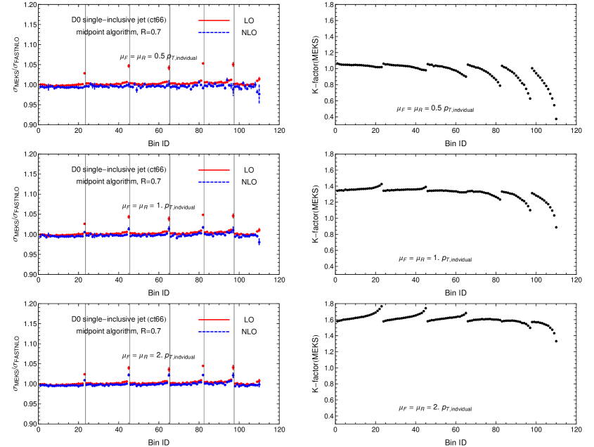
Figs. 2-7 compare our representative numerical results with the ones provided by FastNLO 1.0 [18] for the distributions of single-inclusive jets, the invariant mass distributions of dijets, and (in the case of D0 Run-2) the angular distributions () of dijets. Kinematical bins of the Tevatron () [30, 31, 32, 33] and LHC () [11, 12] measurements, and CTEQ6.6 central PDFs [34] were used. For this benchmark comparison, we use the Midpoint algorithm at the Tevatron and anti- algorithm at the LHC. The cone size is indicated in the figures. The central scales are set to the individual jet in the single-inclusive jet production and the average of the two leading jets in dijet production, in accordance with the experimental measurements. We use the 4D recombination scheme. The comparison to the recombination scheme is included at the end of this section.
In Table. 2, we summarize the performance of the program for these representative calculations at NLO as well as LO (shown by values in parentheses). The elapsed CPU time and the achieved numerical accuracy are shown for a single job with one iteration run on a 2.5-GHz Intel Xeon processor. is the total number of experimental bins for each calculation. The integration errors are averaged over all the bins. As was mentioned, the user can run parallel jobs and combine the results at the end, in which case the numerical errors go down proportionally to , where is the total number of iterations in all jobs.
| Exp. ID | Descriptions | CPU time (in mins.) | Numerical errors | |
|---|---|---|---|---|
| 1 | CDF inclusive jet | 72 | 75(2.5) | 8(2)% |
| 2 | D0 inclusive jet | 110 | 114(3.8) | 6(2)% |
| 3 | D0 dijet mass | 71 | 146(3.8) | 5(2)% |
| 4 | D0 dijet angular | 120 | 197(3.4) | 5(1)% |
| 5 | CMS inclusive jet | 176 | 477(15.0) | 8(1)% |
| 6 | CMS dijet mass | 125 | 357(10.7) | 6(1)% |
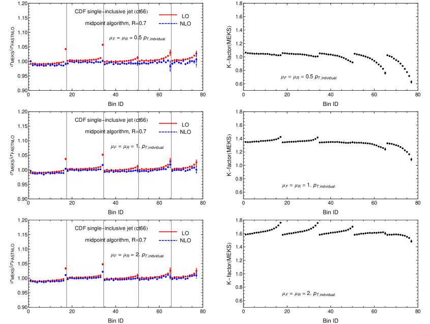
In Figs. 2-7, left panels show ratios of MEKS to FastNLO cross sections, , at LO (red points with error bars) and NLO = LO + NLO-correction (blue points with error bars), in kinematical bins provided by the experiments. The horizontal axis indicates the ID of each bin, which are arranged in the order of increasing jet rapidity and then the jet’s or for the single-inclusive jet and dijet mass measurements, or then for the dijet angular measurement. Vertical lines indicate the boundaries of each rapidity or invariant mass interval. For example, Fig. 2 shows in 6 bins of jet rapidity, with bins 1…23 corresponding to the first rapidity bin (), bins 24…45 corresponding to the second rapidity bin (), and so on. The left panel includes, from top to bottom, three plots obtained with the renormalization and factorization scales equal to 1/2, 1, and 2 times the central scale. We can see a good overall agreement between MEKS and FastNLO both at LO and NLO. The only significant discrepancies are found in the highest bins for both the Tevatron and LHC single-inclusive jet production, which are due to the difference in the scale choices used in MEKS and FastNLO 1.0. [These differences reduce when going to NLO]. In the MEKS single-inclusive jet calculation, we use the actual of the partonic jet filled into the bin as the scale input. FastNLO 1.0 sets the scale according to a fixed value in each experimental bin, which tends to be different from the actual of the jet in the highest bins, which have large widths. The same reason causes a small normalization shift in other bins. For dijet production, we only observe random fluctuations at highest that are mainly due to numerical integration errors. There is a new version of FastNLO, FastNLO 2.0 [35], in which the scale is no longer set to a fixed value in each bin. The tables for this version are not available for the Tevatron jet cross sections, but they are available for the ATLAS and CMS single-inclusive jet cross sections. When we used FastNLO 2.0 for the cross sections in Fig. 6, we find much better agreement with our MEKS results.
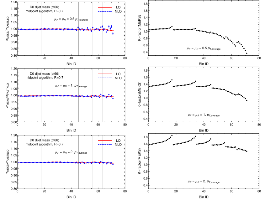
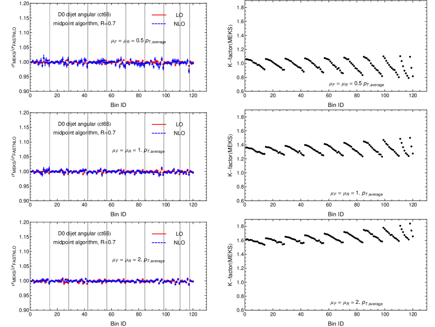
As a practical application, we wish to examine the sensitivity of the NLO cross section to the choice of the QCD scales and . In the right panels of Figs. 2-7, for each distribution, we present plots using MEKS of the NLO K factor, defined as the ratio of the NLO differential cross section to the LO one. The value of the K factor and its stability with respect to the scale choice may provide an indication of the magnitude of yet higher-order corrections. To minimize the potential effect of higher-order terms, one might opt to choose the renormalization and factorization scales that bring the K factor close to unity in most of the kinematical region. An alternative approach for setting the scale is based on the minimal sensitivity method, which suggests to choose the and values (taken to be equal and designated as in the following) at the point where the scale dependence of the NLO cross section is the smallest.
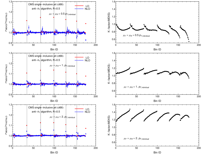
In (di)jet production at central rapidities at the Tevatron, both requirements (and ) could be satisfied by choosing ; see, e.g., the appendix in Ref. [36]. However, the point of the minimal sensitivity shifts to higher values (close to or even higher) at forward rapidities at the Tevatron or at all rapidities at the LHC. For such higher scales, however, it is hard to satisfy the requirement that remains close to unity at the same time. This point is illustrated by our plots of the factors. At the central rapidities and at the Tevatron (the lowest 3 rapidity bins in Figs. 2-5), and is relatively independent of , as seen in the top subpanels. However, with this scale choice the factor deviates significantly from unity and has strong kinematic dependence if the rapidity and are large. If one chooses the scale that is equal to or even (the middle and bottom figures), in accord with the minimal sensitivity method for the forward bins, the kinematical dependence of the factor reduces, but its value increases to 1.3-1.6 in most of the bins.
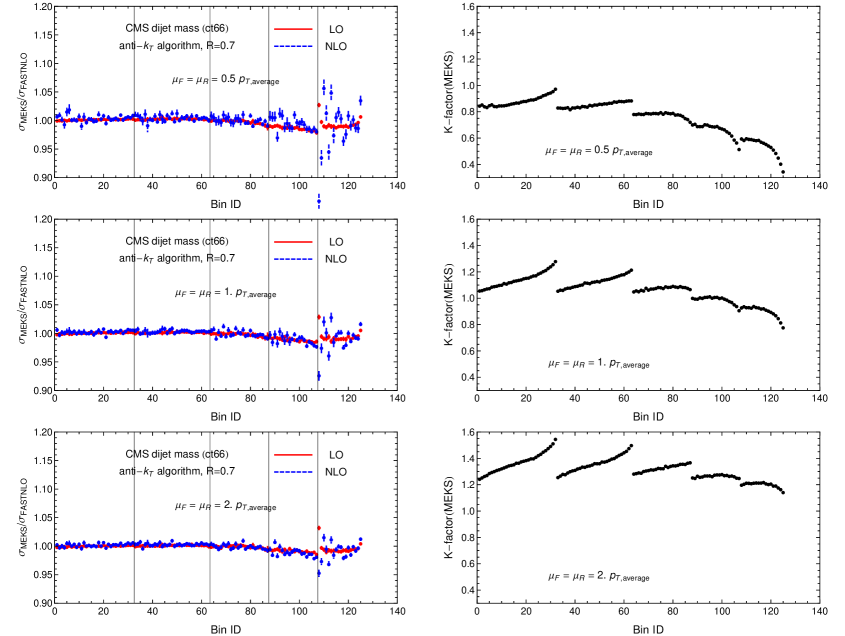
For CMS kinematics (Figs. 6-7), the factor has significant kinematical dependence for all central scale choices, however, the choice (the middle subpanels) results in a comparatively flatter factor that is also closer to unity. We can see that it is hard to find a fixed scale (or a scale of the type [13]) that would simultaneously reduce the magnitude of the NLO correction and stabilize its scale dependence and kinematical dependence. The scale may be slightly more optimal at the Tevatron, and the scale may be slightly better at the LHC.
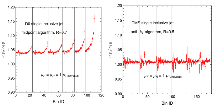
As a final comparison, in Figs. 8 and 9, we plot the ratios of the NLO distributions calculated using different recombination schemes, where is obtained with the 4D scheme, and is with the scheme. For single-inclusive jet production at both the Tevatron and LHC, is larger than . An opposite trend is observed in dijet production. Differences of the predictions based on the two schemes are larger with the Midpoint algorithm (used at the Tevatron) than with the anti- algorithm (used at the LHC). In a NLO calculation, the Midpoint algorithm allows a larger maximal angular separation (2) between the two partons forming a jet, compared to the anti- algorithm that only allows the angular separation up to . This produces the observed different behaviors of the two jet algorithms.
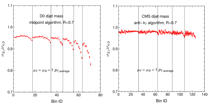
5 Conclusion
In conclusion, this document describes the upgraded EKS program (MEKS) that provides a fast and stable NLO calculation of double-differential cross sections for single-inclusive jet and dijet production at hadron colliders. The new program uses the VEGAS Monte Carlo sampling and the EKS function to generate weighted events and fill them into finely binned two-dimensional histograms for a later analysis. It also includes a user interface to add new jet observables, which is advantageous compared to the popular FastNLO code [18, 19] that provides only the cross sections in the bins of the already completed measurements. Distributions of sample events are tuned automatically to speed up convergence of the integration of steep differential distributions. The program allows parallelization of the Monte-Carlo integration. In order to facilitate the precision comparison of the MEKS code with other existing codes for computations of NLO cross sections, we document a benchmark comparison of the MEKS and FastNLO, and find good agreement. The MEKS code is available at the webpage http://www.hepforge.org/downloads/meks.
ACKNOWLEDGMENTS
This work was supported by the U.S. DOE Early Career Research Award DE-SC0003870 and by Lightner-Sams Foundation; by the U.S. Department of Energy under Grant No. DE-FG02-96ER40969; by the U.S. National Science Foundation under Grant No. PHY-0855561; by the National Science Council of Taiwan under Grant Nos. NSC-98-2112-M-133-002-MY3 and NSC-101-2112-M-133-001-MY3. PMN appreciates helpful discussions of benchmark comparison with J. Huston, J. Rojo, and M. Wobisch. PMN and DES also benefited from discussing related work with participants of the Workshop “High Energy QCD at the start of the LHC” at the Galileo Galilei Institute of Theoretical Physics (INFN Florence, September 2011); they thank the organizers of this workshop for financial support and hospitality. HLL thanks the hospitality of the department of Physics and Astronomy at Michigan State University, where part of this work was done.
References
- [1] V. M. Abazov et. al.,, D0 Collaboration Phys. Rev. D80 (2009) 111107.
- [2] H.-L. Lai et. al., Phys. Rev. D82 (2010) 074024.
- [3] M. Guzzi et. al., arXiv:1101.0561 [hep-ph].
- [4] A. D. Martin, W. J. Stirling, R. S. Thorne, and G. Watt, Eur. Phys. J. C63 (2009) 189.
- [5] R. D. Ball et. al., Nucl. Phys. B838 (2010) 136–206.
- [6] Z. Liang and P. Nadolsky, arXiv:1203.6803 [hep-ph], p. 36.
- [7] S. Chatrchyan et. al.,, CMS Collaboration Phys. Lett. B704 (2011) 123.
- [8] V. Khachatryan et. al.,, CMS Collaboration Phys. Rev. Lett. 106 (2011) 201804.
- [9] G. Aad et. al.,, ATLAS Collaboration New J. Phys. 13 (2011) 053044.
- [10] G. Aad et. al.,, ATLAS Collaboration Eur. Phys. J. C71 (2011) 1512.
- [11] S. Chatrchyan et. al.,, CMS Collaboration Phys. Lett. B700 (2011) 187.
- [12] S. Chatrchyan et. al.,, CMS Collaboration Phys. Rev. Lett. 107 (2011) 132001.
- [13] S. D. Ellis, Z. Kunszt, and D. E. Soper, Phys. Rev. Lett. 69 (1992) 1496.
- [14] Z. Kunszt, and D. E. Soper, Phys. Rev. D46 (1992) 192.
- [15] Z. Nagy, Phys. Rev. Lett. 88 (2002) 122003.
- [16] Z. Nagy, Phys. Rev. D68 (2003) 094002.
- [17] N. Kidonakis and J. F. Owens, Phys. Rev. D63 (2001) 054019.
- [18] T. Kluge, K. Rabbertz, and M. Wobisch, hep-ph/0609285.
- [19] See http://projects.hepforge.org/fastnlo/form/index.html.
- [20] S. Alioli, K. Hamilton, P. Nason, C. Oleari, and E. Re, JHEP 04 (2011) 081.
- [21] T. Hahn, Comput. Phys. Commun. 168 (2005) 78.
- [22] G. P. Lepage, J. Comput. Phys. 27 (1978) 192.
- [23] G. C. Blazey et. al., hep-ex/0005012.
- [24] M. Cacciari, G. P. Salam, and G. Soyez, JHEP 04 (2008) 063.
- [25] S. Catani, Y. L. Dokshitzer, M. H. Seymour, and B. R. Webber, Nucl. Phys. B406 (1993) 187.
- [26] S. D. Ellis and D. E. Soper, Phys. Rev. D48 (1993) 3160.
- [27] Y. L. Dokshitzer, G. D. Leder, S. Moretti and B. R. Webber, JHEP 08 (1997) 001.
- [28] G. P. Salam, Eur. Phys. J. C67 (2010) 637.
- [29] M. R. Whalley, D. Bourilkov, and R. C. Group, hep-ph/0508110. The latest LHAPDF library can be downloaded from http://hepforge.cedar.ac.uk/lhapdf/ .
- [30] V. M. Abazov et. al.,, D0 Collaboration Phys. Rev. Lett. 101 (2008) 062001.
- [31] T. Aaltonen et. al.,, CDF Collaboration Phys. Rev. D78 (2008) 052006.
- [32] V. M. Abazov et. al.,, D0 Collaboration Phys. Lett. B693 (2010) 531.
- [33] V. Abazov et. al.,, D0 Collaboration Phys.Rev.Lett. 103 (2009) 191803.
- [34] P. M. Nadolsky et. al., Phys. Rev. D78 (2008) 013004.
- [35] M. Wobisch et al. [fastNLO Collaboration], arXiv:1109.1310 [hep-ph].
- [36] D. Stump, J. Huston, J. Pumplin, W.-K. Tung, H.-L. Lai, S. Kuhlmann, and J. F. Owens, JHEP 0310 (2003) 046.