Wind driven 3D Navier-Stokes circulation in the Atlantic

Abstract

A finite element method for the numerical solution of the anisotropic Navier-Stokes equations in shallow domain is presented. This method take into account aspect ratio in the hydrostatic approximation of the Navier-Stokes equations [4, 2, 3]. A projection method [7, 15] is used for the time discretization. The linear systems are solved via a some preconditioned conjugate algorithm, well adapted to massively parallel computers [17, 16, 18]. Some results are presented for the wind driven water circulation in the North Atlantic.

Keywords Navier-Stokes equations, shallow water, projection methods, parallel numerical linear algebra, preconditioned conjugate gradient.

1 Introduction

The numerical simulation of wind-driven currents in the ocean is a common and current subject. Most of the used models are based on the hydrostatic approximation and anisotropic viscosity. A Galerkin method for the primitive equations in shallow domains is presented in [10, 11]. Prismatic finite elements are used, and numerical example are presented for the English Channel. In [6], a baroclinic circulation model for the North Atlantic is presented. Spherical-polar coordinated are used . A study of the interaction between a baroclinic and a barotropic model is given in [12]. It is based on the planetary geostrophic equations. Finally in [20] a barotropic model is used for the study of the wind-driven circulation in an elongated basin. Most of the anisotropic models used in oceanography can be mathematically justified; see e.g. [4, 2, 19, 3].

Since the publication of the M.S. Lozier paper: Deconstructing the Conveyor Belt [9], it is of importance to have a good description of the wind-driven circulation in oceans. This paper is devoted to the numerical simulation of such a circulation in the North Atlantic, with a particular attention to the 3D aspects; including down and up-welling.

In this paper, the full system of Navier-Stokes equations is considered; it is organized as follows. In section 2, we recall the setting of the anisotropic Navier-Stokes equations in the context of thin domains. Then a description of a projection method is presented in section 3. A weak formulation and a finite element discretization are given in sections 4 and 5. We end this paper with section 6 where some numerical simulations obtained with our method are presented. Some wind driven 3D Navier-Stokes circulation in the North Atlantic is reported.

2 Anisotropic Navier-Stokes equations

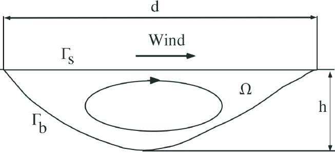
Water flows in oceanography and limnology are governed by the Navier-Stokes equations. For some numerical simulations, asymptotic models are in current use (see [13, 21]). These are all based on the fact that the horizontal dimensions of the considered domain are much larger than the vertical one. Let $d$ be the horizontal width, and $h$ be the depth. The simplest model using the fact that

$$\epsilon=\frac{h}{d}$$

is very small is the hydrostatic model. In this model, we take care of turbulence effects by setting an anisotropic viscosity, much smaller in the vertical direction than in the horizontal one (see [13]).

Let $\Omega=\Omega_{\epsilon}\subset\mathbb{R}^{3}$ be the domain defined by

$$\Omega=\left\{{x=(x_{1},x_{2},x_{3})\in\mathbb{R}^{3},\;(x_{1},x_{2})\in\Gamma_{s},\;-h(x_{1},x_{2})<x_{3}<0}\right\}$$

where $\Gamma_{s}$ is the surface of the domain and $h:\Gamma_{s}\rightarrow\mathbb{R}$ is its depth. The bottom of the domain is defined by $\Gamma_{b}=\partial\Omega\setminus\Gamma_{s}$ (Fig. 1).

Figure 1: Illustration of the shallow domain

It is assumed that the water motion is generated by horizontal tension, induced by some wind on the surface $\Gamma_{s}$. This motion is driven by the following anisotropic Navier-Stokes equations and is influenced by the Coriolis force:

$$u_{t}+\left({u}\mid{\nabla}\right)u = \Delta_{\nu}u-2\omega\wedge u-\nabla p\quad{\rm in\;\Omega},\;t>0,$$ (1)

$$\mathop{\rm div}\nolimits\,u = 0\quad{\rm in}\;\Omega,\;t>0,$$ (2)

with the following boundary and initial conditions. The bottom $\Gamma_{b}$ is subdivided into two parts $\Gamma_{0}$ with strictly positive measure, and $\Gamma_{1}=\Gamma_{b}\setminus\Gamma_{0}$, and

$$u=0\quad{\rm on}\;\Gamma_{0},\;t>0,$$ (3)

$$\left({u}\mid{n}\right)=0,\;\left({\sigma\cdot n}\mid{\tau}\right)=0\quad{\rm on}\;\Gamma_{1},\;t>0,$$ (4)

where $\sigma=\sigma_{ij}$ is the stress tensor, with $\sigma=-pI+\nabla u\cdot\nu+\nu\cdot\nabla u^{t}$, $n$ is the unit outward normal vector to the boundary, and $\tau$ is any tangential vector. Note that the part $\Gamma_{1}$ of the bottom corresponds to artificial limits of the domain.

On the surface $\Gamma_{s}$, tension conditions are considered

$$\nu_{3}\frac{\partial{u_{1}}}{\partial{x_{3}}}=\theta_{1},\quad\nu_{3}\frac{\partial{u_{2}}}{\partial{x_{3}}}=\theta_{2},\quad u_{3}=0\quad{\rm on}\;\Gamma_{s},\;t>0.$$ (5)

Finally the initial condition is

$$u(\cdot,\,t=0)=0\quad{\rm in}\;\Omega.$$ (6)

The following notations have been used: $u=(u_{1},u_{2},u_{3})$ is the fluid velocity, $\omega=(0,0,\omega_{3})$ is the angular velocity of the Earth (projected onto the vertical in local coordinates), $p$ is the pressure, $\nu=\mathrm{diag}(\nu_{1},\nu_{2},\nu_{3})$ is the turbulent viscosity diagonal tensor, $\theta_{1}$ and $\theta_{2}$ are the tensions induced by the wind and

$$\Delta_{\nu}\varphi=\sum_{j=1}^{3}\;\nu_{j}\;\frac{{\partial}^{2}{\varphi}}{\partial{x_{j}}^{2}}.$$

Let us do the following change of variables and functions

$$x_{1}:=x_{1},\quad x_{2}:=x_{2},\quad x_{3}:=x_{3}/\epsilon$$

$$v_{1}:=u_{1},\quad v_{2}:=u_{2},\quad v_{3}:=u_{3}/\epsilon$$

With this scale change we get

$$\frac{\partial{v_{1}}}{\partial{t}}+\left({v}\mid{\nabla v_{1}}\right)-\Delta_{{\nu}^{\epsilon}}v_{1}-fv_{2}+\frac{\partial{p}}{\partial{x_{1}}} = 0\quad{\rm in}\;\Omega,\;t>0,$$

$$\frac{\partial{v_{2}}}{\partial{t}}+\left({v}\mid{\nabla v_{2}}\right)-\Delta_{{\nu}^{\epsilon}}v_{2}+fv_{1}+\frac{\partial{p}}{\partial{x_{2}}} = 0\quad{\rm in}\;\Omega,\;t>0,$$

$${\epsilon}^{2}\;\{\frac{\partial{v_{3}}}{\partial{t}}+\left({v}\mid{\nabla v_{3}}\right)-\Delta_{{\nu}^{\epsilon}}v_{3}\}+\frac{\partial{p}}{\partial{x_{3}}} = 0\quad{\rm in}\;\Omega,\;t>0,$$

$$\mathop{\rm div}\nolimits\,v = 0\quad{\rm in}\;\Omega,\;t>0,$$

$${\nu}_{3}\frac{\partial{v_{1}}}{\partial{x_{3}}}=\epsilon\theta_{1},\quad\nu_{3}\frac{\partial{v_{2}}}{\partial{x_{3}}}=\epsilon\theta_{2},\quad v_{3}=0\quad{\rm on}\;{\Gamma}_{s},\;t>0,$$

$$v=0\quad{\rm on}\;\Gamma_{0},\;t>0,$$

$$\left({v}\mid{n}\right)=0,\;\left({\sigma_{\epsilon}\cdot n}\mid{\tau}\right)=0\quad{\rm on}\;\Gamma_{1},\;t>0,$$

with ${\nu}^{\epsilon}=\mathrm{diag}({\nu}_{1},{\nu}_{2},{\nu_{3}}/{\epsilon^{2}})$, and $f=2{\omega}_{3}$.
Set

$$\nu_{1}=\lambda_{1},\;\nu_{2}=\lambda_{2},\;\nu_{3}=\epsilon^{2}\,\lambda_{3},$$

$$\Theta_{i}=\epsilon^{-1}\,\theta_{i}\;\;\;i=1,2,$$

$$\lambda=(\lambda_{1},\lambda_{2},\lambda_{3}).$$

When $\epsilon\rightarrow 0$, this problem becomes the hydrostatic approximation of Navier-Stokes equations.

$$\frac{\partial{v_{1}}}{\partial{t}}+\left({v}\mid{\nabla v_{1}}\right)-\Delta_{{\lambda}}v_{1}-fv_{2}+\frac{\partial{p}}{\partial{x_{1}}} = 0\quad{\rm in}\;\Omega,\;t>0,$$ (7)

$$\frac{\partial{v_{2}}}{\partial{t}}+\left({v}\mid{\nabla v_{2}}\right)-\Delta_{\lambda}v_{2}+fv_{1}+\frac{\partial{p}}{\partial{x_{2}}} = 0\quad{\rm in}\;\Omega,\;t>0,$$ (8)

$$\frac{\partial{p}}{\partial{x_{3}}} = 0\quad{\rm in}\;\Omega,\;t>0,$$ (9)

$$\mathop{\rm div}\nolimits v = 0\quad{\rm in}\;\Omega,\;t>0.$$ (10)

with

$$v_{1}=v_{2}=v_{3}\cdot n_{3}=0\quad{\rm on}\;{\Gamma}_{0},\;t>0,$$ (11)

$$\left({v_{H}}\mid{n_{H}}\right)=0,\;\left({\sigma_{H}\cdot n_{H}}\mid{\tau_{H}}\right)=0\quad{\rm on}\;\Gamma_{1},\;t>0,$$ (12)

where $w_{H}$ denotes the horizontal components of $w$,

$${\lambda}_{3}\frac{\partial{v_{1}}}{\partial{x_{3}}}=\Theta_{1},\quad\lambda_{3}\frac{\partial{v_{2}}}{\partial{x_{3}}}=\Theta_{2},\quad v_{3}=0\quad{\rm on}\;{\Gamma}_{s},\;t>0,$$ (13)

$$v_{1}(\cdot,\,t=0)=v_{2}(\cdot,\,t=0)=0\quad{\rm in}\;\Omega.$$ (14)

This development shows that it is natural to use an anisotropic viscosity diagonal tensor with the third component of the order of $\epsilon^{2}$, compared with the others.

3 Projection method

In order to solve equations (1)-(6), a velocity-correction projection method [7, 15, 8] is used. Let us recall this method in our case. Set $u^{0}=u(0),p^{0}=p(0)$, and let $u^{1}$, and $p^{1}$ be approximations of $u(\delta t)$ and $p(\delta t)$. A BDF2 scheme is used for the time discretization. For $k\geq 1$, we look for $\tilde{u}^{k+1},p^{k+1}$, and $u^{k+1}$ such that the prediction $\tilde{u}^{k+1}$ of the velocity is a solution of

$$\frac{1}{\delta t}\left(\frac{3}{2}\tilde{u}^{k+1}-2u^{k}+\frac{1}{2}u^{k-1}\right)-\Delta_{\nu}\tilde{u}^{k+1} = -\left({u^{k}}\mid{\nabla}\right)u^{k}-2\omega\wedge u^{k}-\nabla p^{k}\;\text{ in }\Omega,$$ (15)

$$\tilde{u}^{k+1} = 0\;\text{ on }\Gamma_{0},$$ (16)

$$\left({\tilde{u}^{k+1}}\mid{n}\right) = 0\;\text{ on }\Gamma_{1},$$ (17)

$$\nu_{3}\frac{\partial\tilde{u}_{1}^{k+1}}{\partial x_{3}} = \theta_{1}^{k+1},\;\text{ on }\Gamma_{s}$$ (18)

$$\nu_{3}\frac{\partial\tilde{u}_{2}^{k+1}}{\partial x_{3}} = \theta_{2}^{k+1},\;\text{ on }\Gamma_{s}$$ (19)

$$\tilde{u}_{3}^{k+1} = 0\;\text{ on }\Gamma_{s},$$ (20)

then the velocity $u^{k+1}$, and the pressure $p^{k+1}$ satisfy

$$\frac{3}{2\delta t}\left(u^{k+1}-\tilde{u}^{k+1}\right)+\nabla\left(p^{k+1}-p^{k}\right) = 0\;\text{ in }\Omega,$$ (21)

$$\mathop{\rm div}\nolimits u^{k+1} = 0\;\text{ in }\Omega,$$ (22)

$$\left({u^{k+1}}\mid{n}\right) = 0\;\text{ on }\partial\Omega.$$ (23)

If $q^{k+1}=p^{k+1}-p^{k}$, from equations (21) and (22) we have

$$-\Delta q^{k+1} = -\frac{3}{2\delta t}\mathop{\rm div}\nolimits\tilde{u}^{k+1}\;\text{ in }\Omega,$$ (24)

$$\frac{\partial{q^{k+1}}}{\partial{n}} = 0\;\text{ on }\partial\Omega.$$ (25)

If $q^{k+1}$ is known, then $p^{k+1}=q^{k+1}+p^{k}$, and $\displaystyle u^{k+1}=\tilde{u}^{k+1}+\delta t\frac{2}{3}\nabla q^{k+1}$.

Note that this method consists in computing a non divergence-free prediction $\tilde{u}^{k+1}$ of the velocity, and then obtain $u^{k+1}$ as a divergence-free vector field via a pressure correction.

4 Weak formulation

A week formulation of problems (15)-(20) and (24)-(25) is the following. Define

$$V = \left\{{\varphi\in H^{1}(\Omega);\;\varphi=0\;{\rm on}\;{\Gamma}_{0}}\right\},$$

$$W = \left\{{v\in V^{3};\;\left({v}\mid{n}\right)=0\;{\rm on}\;\Gamma_{s}\cup\Gamma_{1}}\right\},$$

$$U = \left\{{v\in H^{1}(\Omega)^{3};\;\left({v}\mid{n}\right)=0\;{\rm on}\;\partial\Omega}\right\}.$$

For $\theta_{1},\,\theta_{2}\in H^{-1/2}(\Gamma_{s})$, if $k\geq 0$, assume that $p^{k}\in H^{1}(\Omega)/\mathbb{R}$, and $u^{k},u^{k-1}$ in $U$ are given. We seek for $\tilde{u}^{k+1}\in W$ such that

$$\frac{3}{2\delta t}\int_{\Omega}\left({\tilde{u}^{k+1}}\mid{v}\right)\,dx+\int_{\Omega}\left({\nu\cdot\nabla\tilde{u}^{k+1}}\mid{\nabla v}\right)\,dx=\\ \frac{1}{\delta t}\int_{\Omega}\left(2\left({u^{k}}\mid{v}\right)-\frac{1}{2}\left({u^{k-1}}\mid{v}\right)\right)\,dx-\int_{\Omega}\left({\left({u^{k}}\mid{\nabla}\right)u^{k}}\mid{v}\right)\,dx\\ -\int_{\Omega}2\left({\omega\wedge u^{k}}\mid{v}\right)\,dx+\int_{\Omega}p^{k}\,\mathop{\rm div}\nolimits v\,dx+\int_{\Gamma_{s}}\theta_{1}^{k+1}v_{1}\,ds+\int_{\Gamma_{s}}\theta_{2}^{k+1}v_{2}\,ds,$$ (26)

for all $v\in W$. Then find $q^{k+1}\in H^{1}(\Omega)/\mathbb{R}$ such that

$$\int_{\Omega}\left({\nabla q^{k+1}}\mid{\nabla\varphi}\right)\,dx=-\frac{3}{2\delta t}\int_{\Omega}\mathop{\rm div}\nolimits\tilde{u}^{k+1}\varphi\,dx,$$ (27)

for all $\varphi\in H^{1}(\Omega)/\mathbb{R}$. The pressure $p^{k+1}\in H^{1}(\Omega)/\mathbb{R}$ is given by

$$\int_{\Omega}p^{k+1}\varphi\,dx=\int_{\Omega}(q^{k+1}+p^{k})\varphi\,dx,$$ (28)

for all $\varphi\in L^{2}(\Omega)$. Finally the velocity $u^{k+1}\in U$ is the solution of

$$\int_{\Omega}\left({u^{k+1}}\mid{v}\right)\,dx=\int_{\Omega}\left({\tilde{u}^{k+1}}\mid{v}\right)\,dx+\delta t\frac{2}{3}\int_{\Omega}\left({\nabla q^{k+1}}\mid{v}\right)\,dx,$$ (29)

for all $v\in L^{2}(\Omega)^{3}$.

5 Finite element discretization

A finite element mesh $\tau_{h}$ of the domain $\Omega$ into brick elements is considered: $\overline{\Omega}=\cup_{K\in\tau_{h}}K$, where each geometric elements $K$ is an hexahedron. For $1\leq j\leq 3$, set

$$V_{h} = \left\{{\varphi_{h}\in C(\overline{\Omega});\;\varphi_{h}|_{K}\in Q_{2},\;\forall K\in\tau_{h}}\right\},$$

$$W_{h} = \left\{{v_{h}\in V_{h}^{3};\;\left({v_{h}}\mid{n}\right)=0\;{\rm on}\,\Gamma_{s}\cup\Gamma_{1};\;v=0\;{\rm on}\;\Gamma_{0}}\right\},$$

$$U_{h} = \left\{{v_{h}\in V_{h}^{3};\;\left({v_{h}}\mid{n}\right)=0\;{\rm on}\,\partial\Omega}\right\},$$

$$P_{h} = \left\{{\varphi_{h}\in C(\overline{\Omega});\;\varphi_{h}|_{K}\in Q_{1},\;\forall K\in\tau_{h}}\right\}.$$

The following finite element discretization of the previous projection method is used.

For $k\geq 0$, assume that $p^{k}_{h}\in P_{h}$, and $u^{k}_{h},u^{k-1}_{h}$ in $U_{h}$ are given. Then compute $\tilde{u}^{k+1}_{h}\in W_{h}$ such that

$$\frac{3}{2\delta t}\int_{\Omega}\left({\tilde{u}^{k+1}_{h}}\mid{v_{h}}\right)\,dx+\int_{\Omega}\left({\nu\cdot\nabla\tilde{u}^{k+1}_{h}}\mid{\nabla v_{h}}\right)\,dx=\\ \frac{1}{\delta t}\int_{\Omega}\left(2\left({u^{k}_{h}}\mid{v_{h}}\right)-\frac{1}{2}\left({u^{k-1}_{h}}\mid{v_{h}}\right)\right)\,dx-\int_{\Omega}\left({\left({u^{k}_{h}}\mid{\nabla}\right)u^{k}_{h}}\mid{v_{h}}\right)\,dx\\ -\int_{\Omega}2\left({\omega\wedge u^{k}_{h}}\mid{v_{h}}\right)\,dx+\int_{\Omega}p^{k}_{h}\,\mathop{\rm div}\nolimits v_{h}\,dx+\int_{\Gamma_{s}}\theta_{1}^{k+1}v_{h,1}\,ds+\int_{\Gamma_{s}}\theta_{2}^{k+1}v_{h,2}\,ds,$$ (30)

for all $v_{h}\in W_{h}$. Then find $q_{h}^{k+1}\in P_{h}/\mathbb{R}$ with

$$\int_{\Omega}\left({\nabla q_{h}^{k+1}}\mid{\nabla\varphi_{h}}\right)\,dx=-\frac{3}{2\delta t}\int_{\Omega}\mathop{\rm div}\nolimits\tilde{u}^{k+1}_{h}\varphi_{h}\,dx,$$ (31)

for all $\varphi_{h}\in P_{h}$. The pressure $p_{h}^{k+1}\in P_{h}/\mathbb{R}$ is given by

$$\int_{\Omega}p_{k}^{k+1}\varphi_{h}\,dx=\int_{\Omega}(q_{h}^{k+1}+p_{h}^{k})\varphi_{h}\,dx,$$ (32)

for all $\varphi_{h}\in P_{h}$. Finally the velocity $u_{h}^{k+1}\in U_{h}$ is the solution of

$$\int_{\Omega}\left({u_{h}^{k+1}}\mid{v_{h}}\right)\,dx=\int_{\Omega}\left({\tilde{u}^{k+1}_{h}}\mid{v_{h}}\right)\,dx+\delta t\frac{2}{3}\int_{\Omega}\left({\nabla q_{h}^{k+1}}\mid{v_{h}}\right)\,dx,$$ (33)

for all $v\in V_{h}^{3}$.
Remark

1. The solution of the linear systems (30)-(33) are performed via some preconditioned conjugate gradient methods. These methods are well adapted to massively parallel computers.

2. For equation (31), a coupled preconditionner: diagonal plus optimal conjugate Grahm-Schmidt least squares preconditionner (DIAG + LS CGS OPT) is used, see [16, 18, 17]. Moreover a Lagrange multiplier is used in order to impose the zero mean of $q_{h}^{k+1}$, see also [5].

3. For the other equations, an incomplete Cholesky IC0 preconditionner [14] is sufficient.

6 Application to the North Atlantic

This section is devoted to the numerical simulation of the $3D$ water circulation in the North Atlantic ocean, induced by some mean wind tensions. For this, the methods presented in the previous sections are used. A parallel software was developed to solve this kind of problems. The bathymetry, and the wind tensions where obtained from the Mercator Ocean Project (http://www.mercator.fr). We are grateful to Jean-Marc Molines at INP-Grenoble for his help.

The model into consideration does not take into account of the temperature, nor the salinity. Our aim is, in a first step, to study the currents induced by the wind tensions in the ocean. A particular attention is turned on the down, and upwelling near the coast. Our model allows to obtain consistent results with reality. It demonstrate that the winds are the main driving forces for the global dynamic in the oceans.

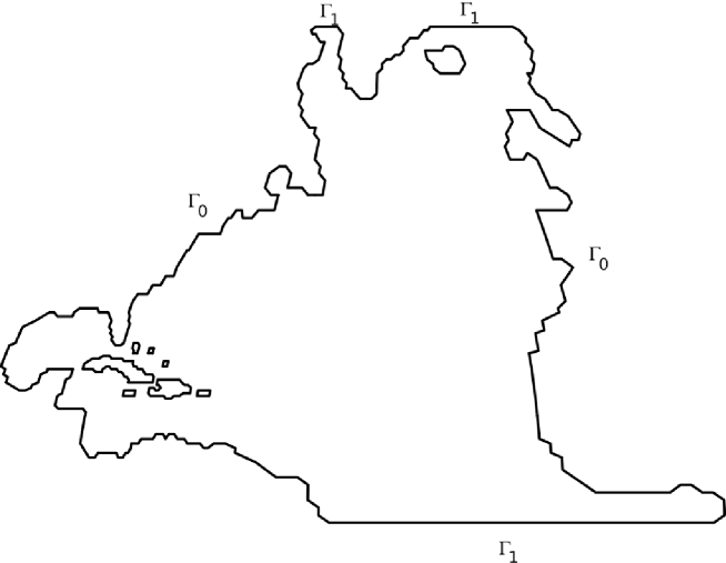
The part of the Atlantic ocean taken into account is delimited in the East by the European and the African continents, in the West by the American continent, in the South by the Equator, and in the North by the $70^{\circ}N$ parallel. These two parts lead to some artificial boundary $\Gamma_{1}$ (see figure 2). On this part of the boundary, it is assumed that there is no tangential tensions, and that there is no water exchange with outside.

Figure 2: Part of the Atlantic Ocean

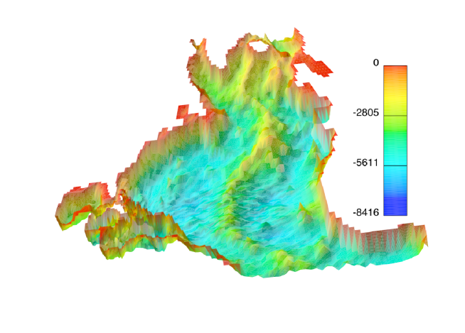
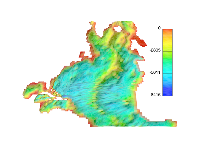
The bathymetry is given in figure 3, and 4.

Figure 3: Bathymetry of the Atlantic Ocean

Figure 4: Bathymetry of the Atlantic Ocean, with vertical scale

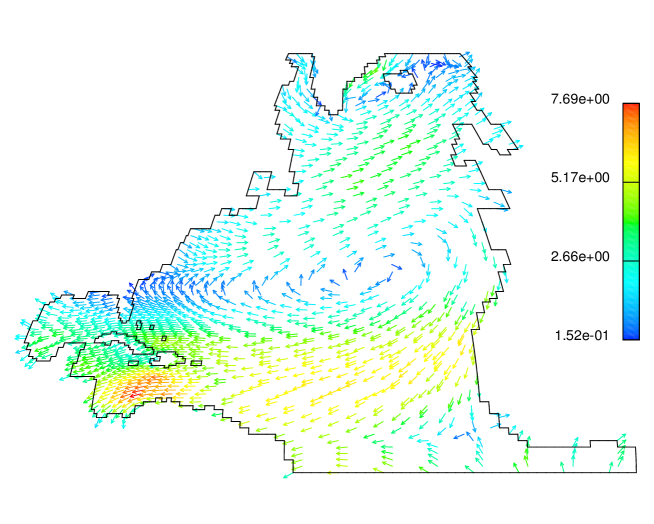
The mean wind during 15 years (1979-1993, ERA15) are represented in figure 5

Figure 5: Mean wind ERA15 (1979-1993)

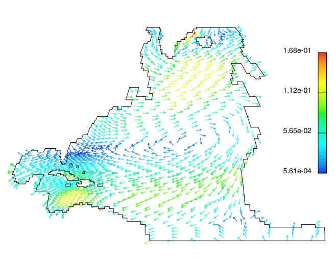
The mean wind tensions during this period are represented in figure 6

Figure 6: Mean wind tensions ERA15 (1979-1993)

The following physical constants are used in the equations:

• The turbulent cinematic viscosity tensor is $\nu=(10^{8},\,10^{8},\,2.5\cdot 10^{2})\;[m^{2}/s]$, it is based on the study of the Reynolds turbulent tensor.

• The time step is $\delta t=2.592\cdot 10^{6}$ (= 1 month).

• The final time is set to 100 years

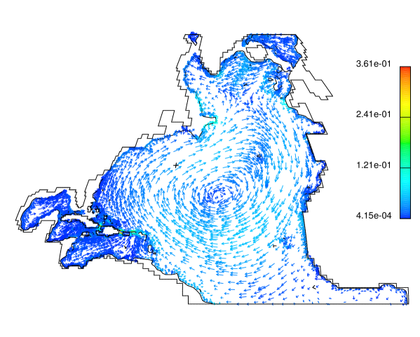
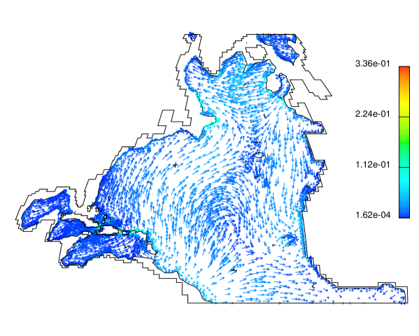
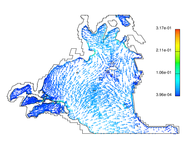
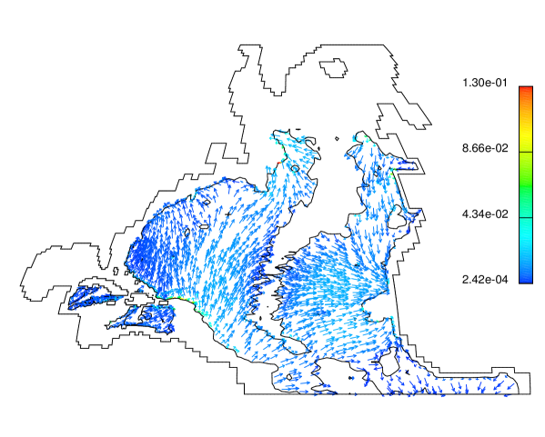
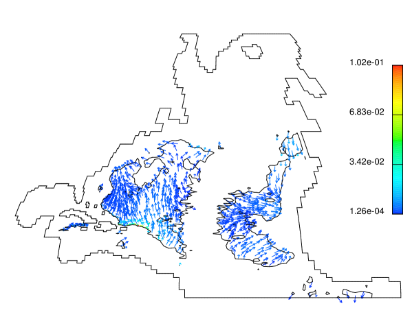
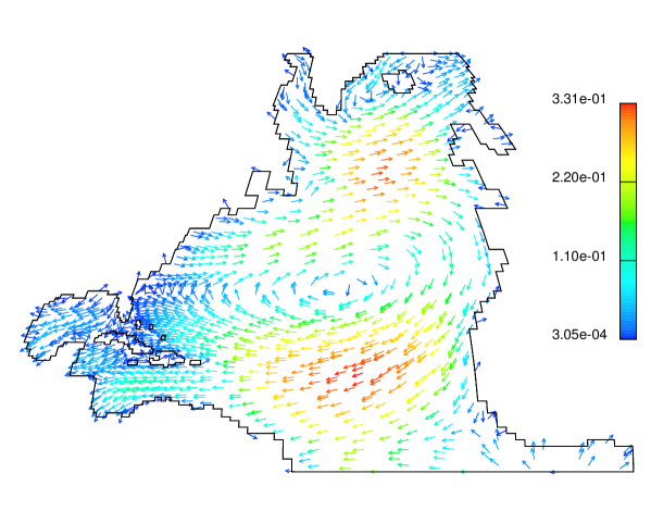
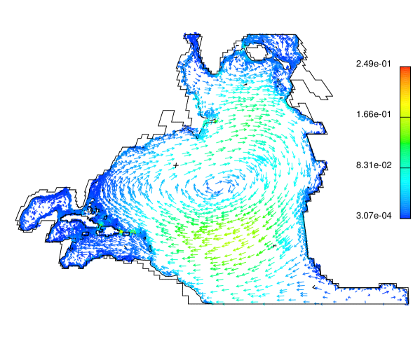
In the following figures, some numerical results for the currents at different depth are presented.

Figure 7: Currents at the surface

Figure 8: Currents at 500 m depth

Figure 9: Currents at 1000 m depth

Figure 10: Currents at 1500 m depth

Figure 11: Currents at 2000 m depth

Figure 12: Currents at 4000 m depth

Figure 13: Currents at 5000 m depth

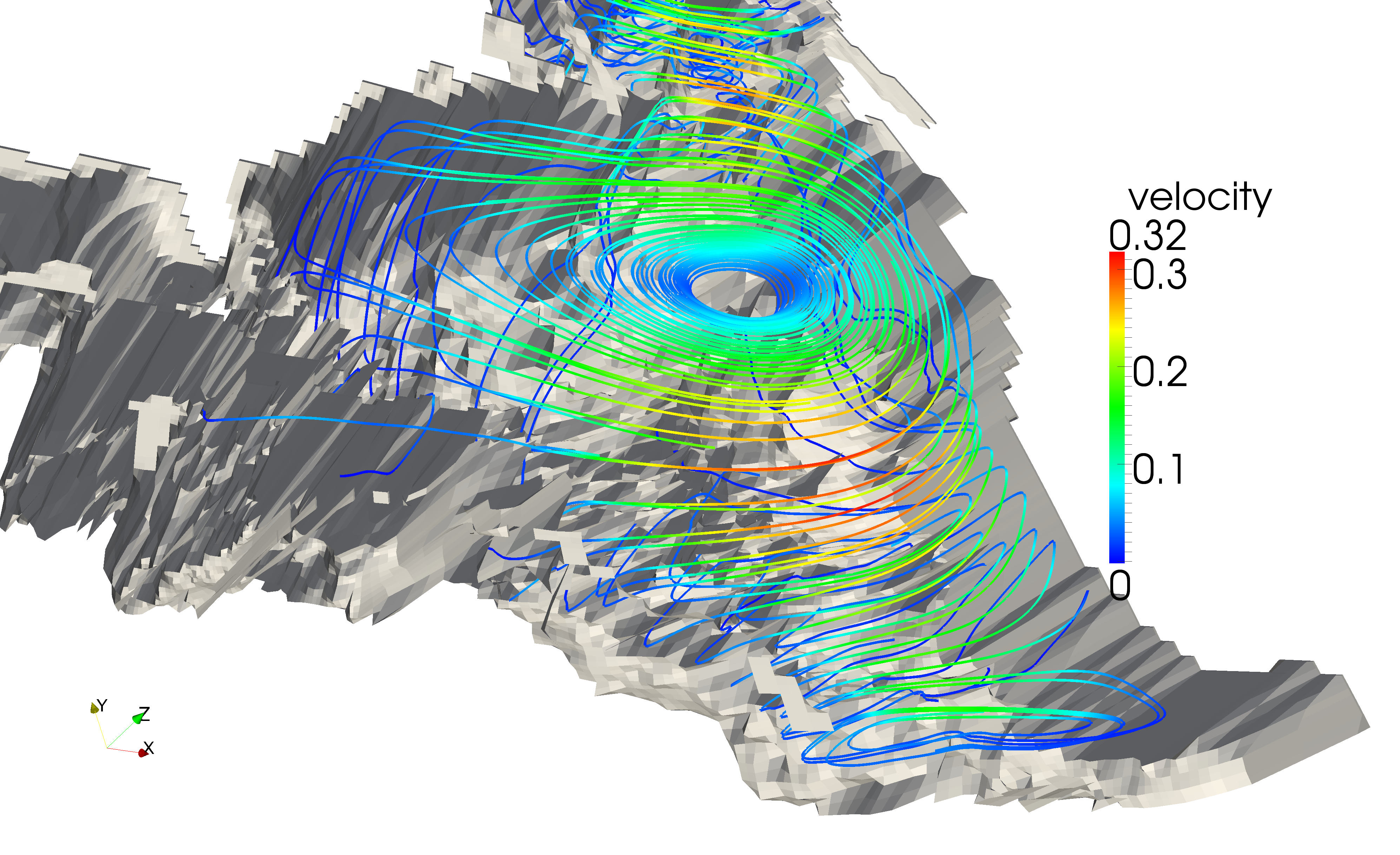
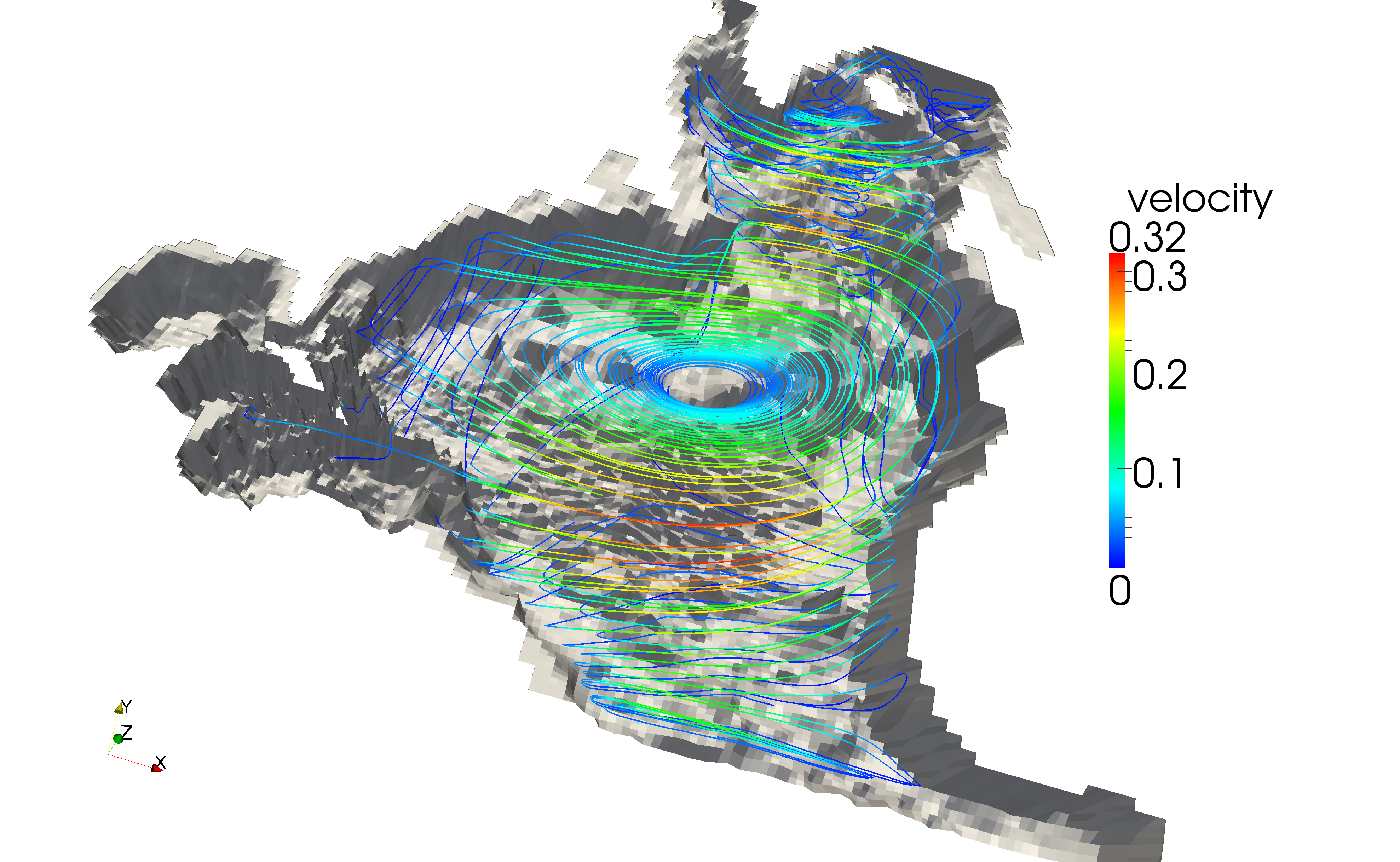
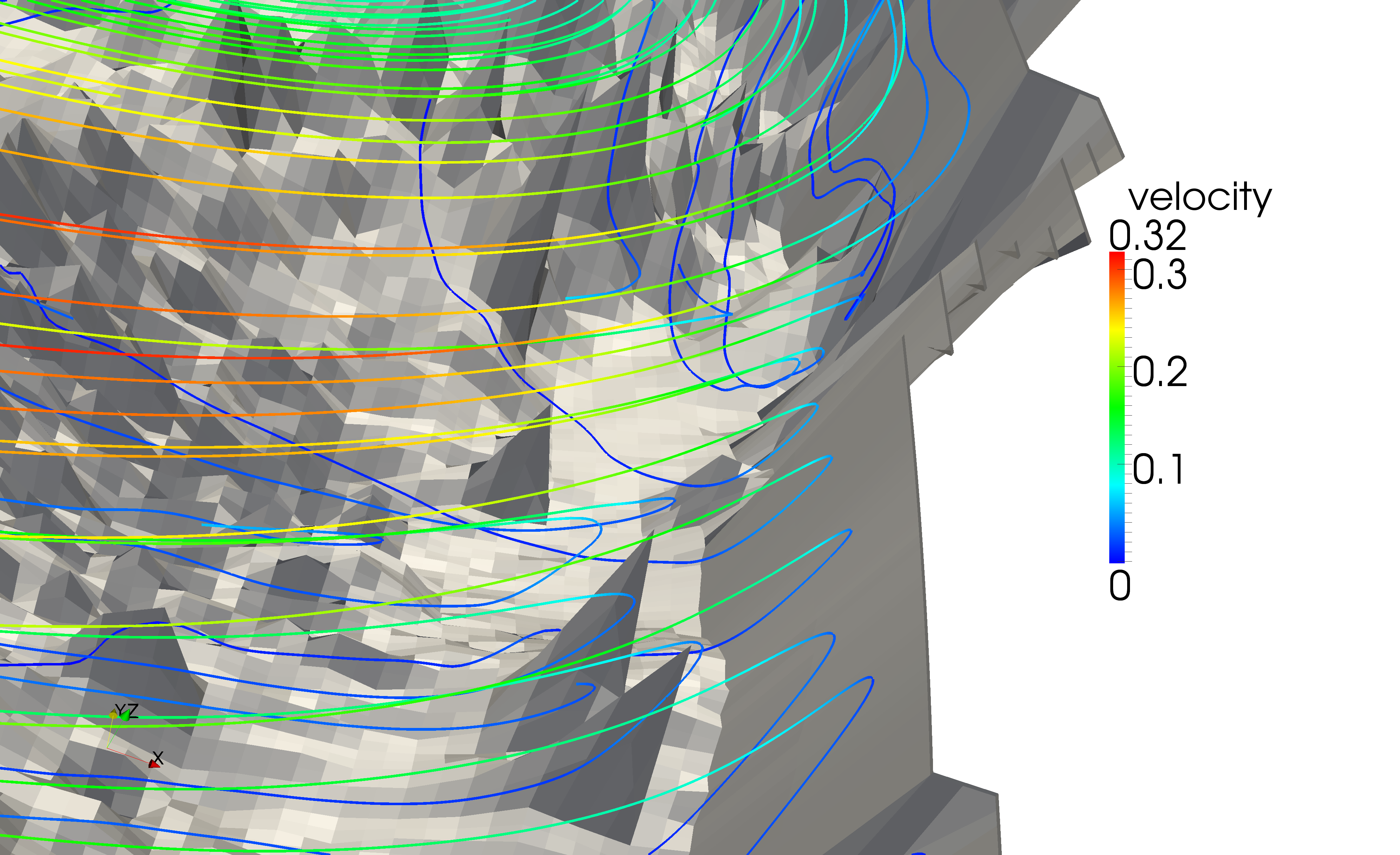
The next figures show the streamlines associated to the previous velocity field. The upwelling and downwelling are shown near the American and the African coasts.

Figure 14: Computed streamlines in the North Atlantic

Figure 15: Upwelling on the African coast

Figure 16: Down and upwelling on the American coast

Let us mention that the travel time for a particle of water, at the surface, to cross the Atlantic from the African coast to the South American coast is about 250 days. The travel time of the same particle to come back from the South American coast to the African one through the deep water is about 12 years.

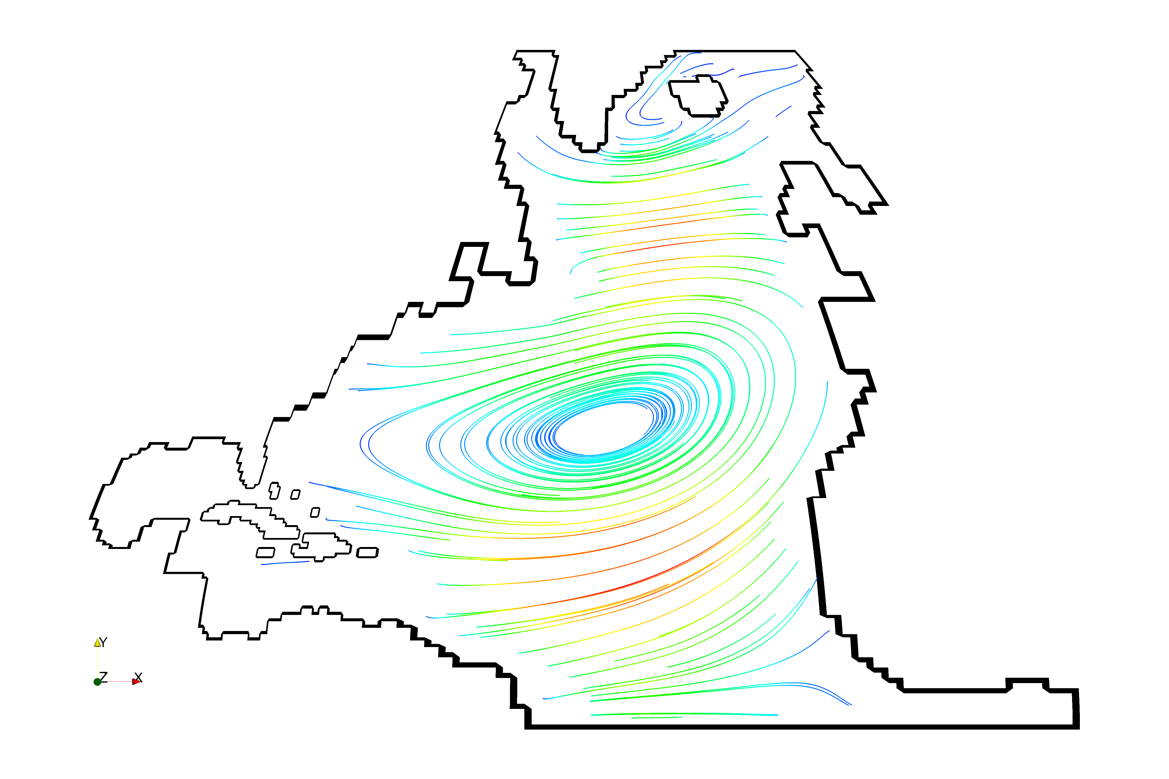
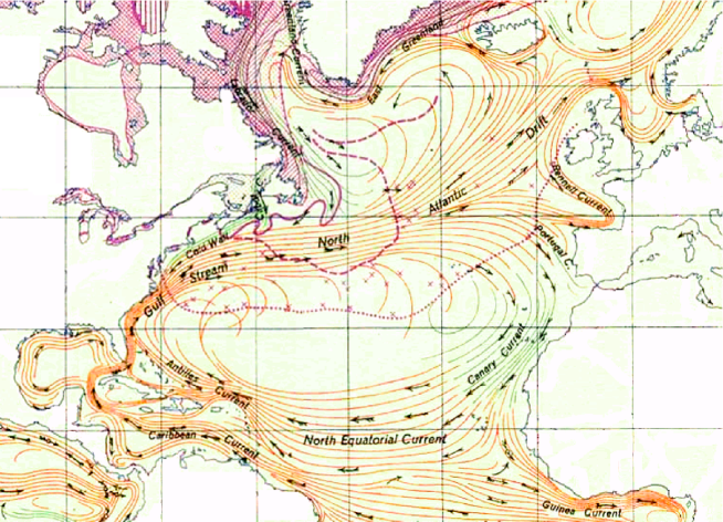
Finally a representation of the surface streamlines obtained with our model is represented in figure 17. This figure can be compared with figure 18 obtained on the web site [1].

The main difference between these two figures are in the region of the Caribbean Islands. The reasons for these differences are

• Our model do not take into account the temperature and the salinity. Therefore we do not have buoyancy effects.

• Because of our boundary conditions on the Equator, we could not take into account of the South Equatorial current along the East coast of South America. For this we could have to compute the currents in the entire Atlantic, but we could not have access to the data for this.

Figure 17: Streamlines at the surface

Figure 18: North Atlantic Gyre [1]

As already mentioned, our model is able to precisely describe the down, and upwelling near the coast. Moreover it allows to obtain consistent results with measurements, and demonstrate that the winds are the main driving forces for the global dynamic in the oceans.
Acknowledgements. We are grateful to the CSCS (Swiss National Supercomputing Center, http://www.cscs.ch) for the use of the computing facilities for a preliminary version of our software. We are also grateful to Mario Valle at CSCS for his hints in the use of graphics softwares.

References

• [1] The north atlantic gyre. World Wide Web electronic publication, 2008. http://commons.wikimedia.org/wiki/File:North_Atlantic_Gyre.png.
• [2] P. Azérad. Equations de Navier-Stokes en bassin peu profond. PhD thesis, Université de Neuchâtel, 1995.
• [3] P. Azérad and F. Guilln-González. Mathematical justification of the hydrostatic approximation in the primitive equations of geophysical fluid dynamics. SIAM J. Math. Anal., 33:847–859, 2001.
• [4] O. Besson and M.R. Laydi. Some estimates for the anisotropic navier-stokes equations and for the hydrostatic approximation. M2AN - Mod. Math. Ana. Num., 26:855–865, 1992.
• [5] P. Bochev and R.B. Lehoucq. On the finite element solution of the pure neumann problem. SIAM Review, 47:50–66, 2005.
• [6] D.A. Greenberg, F.E. Werner, and Lynch. A diagnostic finite element ocean circulation model in spherical-polar coordinates. J. Atmos. Oceanic Technol., 15:942–958, 1998.
• [7] J. Guermond. Some practical implementations of the projection methods for navier-stokes equations. M2AN - Mod. Math. Ana. Num., 30:637–667, 1996.
• [8] J.-L. Guermond and J. Shen. Velocity–correction projection methods for incompressible flows. SIAM J. Numer. Anal., 41(1):112–134, 2003.
• [9] M. S. Lozier. Deconstructing the conveyor belt. Science, 328:1507–1511, 2010.
• [10] D.R. Lynch and F.E. Werner. Three-dimensional hydrodynamics on finite elements. part i: Linearized harmonic model. Int. J. Numer. methiods Fluids, 7:871–909, 1987.
• [11] D.R. Lynch and F.E. Werner. Three-dimensional hydrodynamics on finite elements. part ii: Non-linear time stepping model. Int. J. Numer. methiods Fluids, 12:507–533, 1991.
• [12] D. Olbers and C. Eden. A simplified general circulation model for a baroclinic ocean with topography. part i: Theory, waves and wind-driven circulation. J. Phys. Oceanogr, 33:2719–2737, 2003.
• [13] J. Pedlosky. Geophysical fluid dynamics. Springer-Verlag, 1987.
• [14] Y. Saad. Iterative methods for sparse linear systems. SIAM, 2003.
• [15] J. Shen. On error estimates of the projection methods for navier–stokes equations: Second- order schemes,. math. of Comp., 65:1039–1065, 1996.
• [16] J. Straubhaar. Preconditioners for the conjugate gradient algorithm using gram–schmidt and least squares methods. Internat. J. Comput. Math., 84(1):89–108, 2007.
• [17] J. Straubhaar. Préconditionnement de systèmes linéaires symétriques définis positifs. Application à la simulation numérique d’écoulements océaniques tridimensionnels. PhD thesis, Université de Neuchâtel, 2007.
• [18] J. Straubhaar. Parallel preconditioners for the conjugate gradient algorithm using gram–schmidt and least squares methods. Parallel Comput., 34(10):551–569, 2008.
• [19] R. Temam and M. Ziane. Navier-stokes equations in three-dimensional thin domains with various boundary conditions. Adv. differential equations, 1:499–546, 1996.
• [20] C.D. Winant. Three-dimensional wind-driven flow in an elongated, rotating basin. J. Phys. Oceanogr., 34:462–476, 2004.
• [21] R. Zeytounian. Modélisation asymptotique en mécanique des fluides newtoniens. Springer-Verlag, 1994.