QCD in hadron collisions

Abstract

This talk examines recent progress in collider QCD and some facets of the interplay between these developments and searches for new particles and phenomena at the Tevatron and LHC.

1 Introduction

The past 18 months have seen considerable excitement in the field of collider particle physics. Among the topics that deserve a mention, one might include the measurement of an unexpectedly large $t\bar{t}$ forward-backward asymmetry at the Tevatron [1, 2], CDF’s anomalous bump in W+dijet production [3], the LHC’s exclusion of huge swathes of supersymmetric parameter space [4, 5] and hints of the Higgs boson from both the Tevatron and the LHC [6, 7, 8].

The purpose of this talk is to examine a selection of the past years’ collider–QCD developments, attempting to place them in the context of the above “headline” developments. To guide us through this exercise, let us start by recalling that hard collider events can be broken up into various components: the non-perturbative structure of the proton, e.g. encoded in parton distribution functions and as relevant also to multiple semi-soft interactions; the “hard” process, amenable to fixed-order perturbative calculation, usually involving at most a handful of partons; the fragmentation of those partons, often implemented as a parton shower; and the hadronisation process, by which partons turn into the hadrons that are observed experimentally. All of these elements must be dealt with correctly (and together) if one is to fully predict the properties of events at hadron colliders. We start our examination of recent QCD progress by considering the element that has seen the most concerted effort, namely the hard process.

2 The hard process at next-to-leading order

The hard process is where we make use of a perturbative expansion in the strong coupling constant, $\alpha_{s}$. Given that $\alpha_{s}\sim 0.1$ at the scales of relevance, one might expect that a leading-order (LO) calculation should generally be accurate to within about $10\%$. It is quite straightforward to check whether this is the case across a range of processes with the help of a tool such as NLOJet++ [9], MCFM [10] and VBFNLO [11]. While there are cases where next-to-leading order corrections are modest, for example for the inclusive jet spectrum, quite often one finds that the NLO terms are large: the $Z$-boson $p_{t}$ spectrum sees a $50\%$ correction at NLO; and the jet $p_{t}$ spectrum in events with a $Z$-boson sees a NLO correction of several hundred percent. Sometimes these large corrections can be understood based on simple physical considerations, for example the appearance of new, enhanced topologies at NLO. There is, however, no general understanding of the different sizes of the NLO corrections and so, to obtain a reasonable degree of accuracy for hadron collider predictions, one must usually explicitly calculate the NLO terms.

In recent years, guidance as to which NLO calculations to carry out has come from the many different searches that are being performed. A classic example comes from SUSY searches: gluinos can decay to a squark and antiquark, with the squark then decaying to a quark and unobserved neutralino, so the signature for pair production of gluinos is the presence of four jets and missing energy; an important background is then $Z$ plus 4-jets, where the $Z$-boson decays to neutrinos. One would like to know this background to NLO.

A measure of the difficulty of such a calculation is the number of external legs: $Z$ plus 4-jet production is a $2\to 5$ process. The first hadron-collider NLO calculation was for the Drell-Yan process in 1979, i.e. essentially a $2\to 1$ process [12]. It was not until 1987 that $2\to 2$ processes started to be calculated, including photon+jet [13], heavy-quark pair production [14] and dijet production [15, 16]. $2\to 3$ processes started to follow ten years later, notably $Wb\bar{b}$ production [17]. Extrapolating, it should come as no surprise that it was around 2009 that $2\to 4$ processes began to appear, with two calculations for W+3 jets [18] and three for the production of two heavy $q\bar{q}$ pairs [19].

One might deduce that one should then wait until around 2019 for the background process that we mentioned above, $Z$+4 jets, a $2\to 5$ process. Yet, remarkably, its calculation appeared 8 years ahead of schedule, in 2011 [20] (another $2\to 5$ process, W+4 jets, came out earlier, in 2010 [21], and is in excellent agreement with data, cf. Fig. 1 left). There have even been first calculations of processes with a complexity equivalent to that of a $2\to 6$ process [22]. While it is beyond the scope of this review to describe the many ingenious innovations behind this progress, it should be said that a number have benefited from recent progress in understanding how to fully carry out a 20-year old dream [23] of sewing together tree amplitudes to obtain loop graphs (for more details see [24]).

Figure 1: Left: comparison of measurements and NLO (Blackhat-Sherpa) predictions of $W+n$-jet cross sections v. $n$ [25]. Right: ratio of the $Z+2$-jet to $\gamma+2$-jet cross sections at LO, NLO and with parton showers matched to tree-level calculations, showing excellent stability [26].

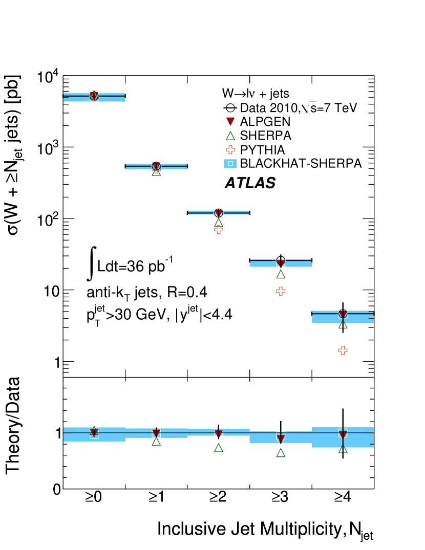
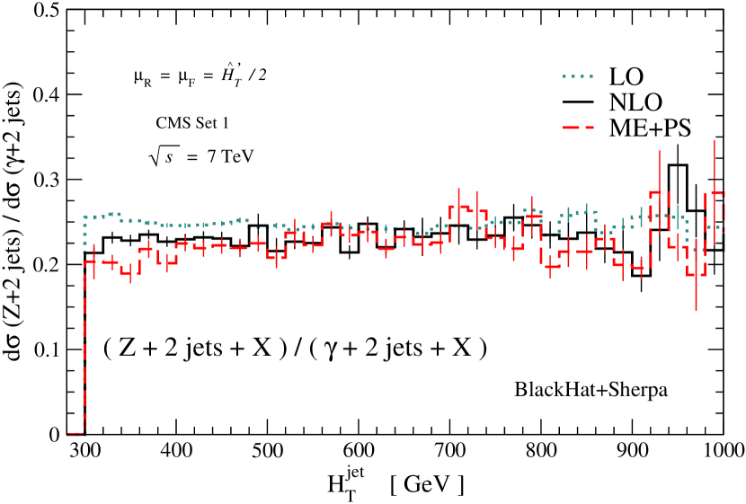
Given this progress, it is natural to ask if it is being used by the experiments. At first sight, when opening one of the many SUSY search papers from ATLAS or CMS one is initially disappointed: nearly all the results rely either on matrix-element (tree-level) calculations supplemented with parton showers (ME+PS) or “data-driven” estimates of backgrounds. Part of the reason is that pure NLO calculations provide information about partons, whereas experiments can only sensibly input hadrons to their detector simulations. Yet, digging deeper, there are cases where cutting-edge NLO results are already having an impact. An example is [27], which compares data both to ME+PS and to data-driven background estimates, relying on the latter for its final SUSY exclusion limits. “Data-driven” sounds as if it is altogether independent of theorists. In this specific case, for estimating the $Z$+jets background the idea is to measure the $\gamma$+jets cross section (instead of a direct measurements of $Z$’s, which suffers from the low $Z\to\ell^{+}\ell^{-}$ branching ratio) and then to use NLO predictions for the ratio of $\gamma$+jets to $Z$+jets to deduce the expected measured $Z$+jets background. Many experimental systematics such as jet-energy scale are common to both and therefore cancel in the ratio; meanwhile the theoretical prediction is extremely stable, Fig. 1 (right). So, the data-driven method here is actually a clever way of exploiting precisely known aspects both theory and experiment, while minimising the impact of their intrinsic limitations. More generally, data-driven methods don’t always (or even often) use NLO, but they do quite often involve this idea of finding a way to combine the best of theory and experiment.

3 Systematically matching showers and NLO

Despite the power of data-driven methods, there remain many cases where the experiments do need a direct, quality prediction of hadron-collider processes. This is crucial in many Higgs searches, which nearly always rely on precise hadron-level predictions of the signal, and also often of the backgrounds. And it was the case also for the analysis that led to the $W$+2-jet anomaly reported by CDF [3], but not found by D0 [28]. One of the standards for collider predictions involves the matching of tree-level matrix-element calculations with parton showers and it is to such predictions, passed through detector simulations, that the CDF and D0 W+2j results were compared.

Combining tree-level (i.e. LO) calculations and parton showers is relatively easy nowadays thanks to automated tools for tree-level predictions of essentially any standard-model process (e.g. MadGraph [29], Alpgen [30], Sherpa [31]) and methods such as MLM [32] and CKKW [33] matching, which address the issue of combining tree-level calculations for different multiplicities, while avoiding the double counting that would be caused by the fact that parton-showers themselves generate extra emissions (for a recent review see [34]).

A concern with any calculation based on tree-level methods is that it is essentially a leading-order calculation, yet we know that NLO corrections can be large. NLO calculations can also be combined with parton showers, through the MC@NLO [35] or POWHEG [36] methods (see also [37]), generally with a significant improvement in precision; this is less straightforward than for tree-level calculations, because of the need for 1-loop matrix-elements and because of extra issues of double counting that arise at NLO. Until recently it had always been done on a case-by-case basis, usually limited to cases with low multiplicities (e.g. just W production, with no jets other than that from the NLO radiation). A major development of the past couple of years has been that a huge number of extra processes has become available. Two approaches have been taken: one is the POWHEG-Box [38], which provides well-documented infrastructure for taking existing NLO calculations and turning them into a POWHEG type calculation (a related approach been taken in Sherpa [39]); the other is the aMC@NLO [40] approach, which builds on MadGraph so as to automatically calculate NLO (loop and tree-level) matrix elements and combine them with parton showers with the MC@NLO method.

x

x

Figure 2: Left: aMC@NLO calculation of the dijet mass spectrum in W+2j events, compared to Alpgen (ME+PS) and pure NLO; also shows are the PDF and scale uncertainties. Right: the CDF data as read from the plots of [3], shown as a ratio to the expected background (also read from the plots), instead of the usual difference between data and background.

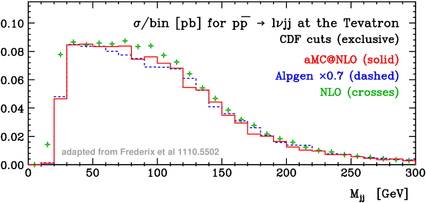
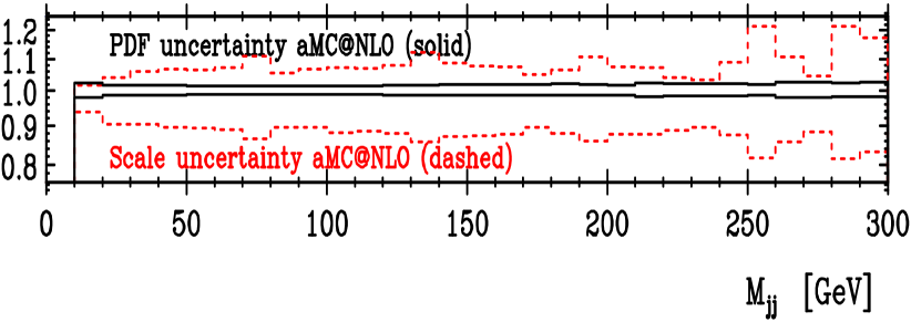
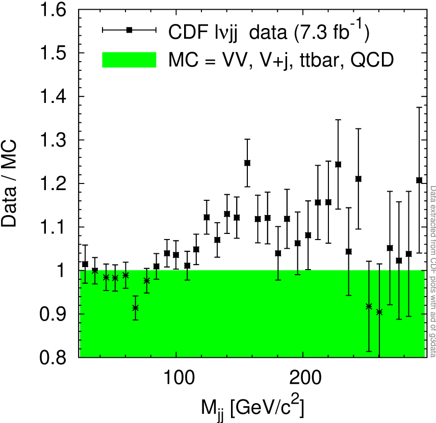
A calculation of the W+2j process with the CDF cuts has been one of the headline applications of the aMC@NLO method, with results shown in Fig. 2 (left). The aMC@NLO and Alpgen results (the latter after a rescaling to account for an overall NLO K-factor) agree remarkably well in this case, suggesting that predictions are relatively stable. Interestingly, aMC@NLO and Alpgen bear more similarity to each other than either does to the pure NLO results, highlighting the importance of showering effects.

One advantage of NLO calculations (whether with a shower or not) is that scale variations can offer a reasonable way of estimating uncertainties. These uncertainties are shown also in Fig. 2 (left) and are of the order of $10-15\%$. For comparison, the right-hand plot of Fig. 2 shows the CDF data as a ratio to the expected background. What appears as a peak around $150\,{\rm GeV}$ in the usual plots of (data$\,-\,$background), here appears as the start of a broad $10\%$ excess starting around $140\,{\rm GeV}$, with only the barest hints of a peak around $150\,{\rm GeV}$. It is not my intention to claim that background uncertainties are responsible for CDF’s anomaly, but simply to provide a reminder that when looking at effects of the order of $10\%$, we enter a region where our ability to predict backgrounds sufficiently accurately can start to become a serious issue. Of course, a number of explanations have been proposed to explain the anomaly (beyond the scope of this talk). Ultimately, however, it is almost certainly impossible for outsiders to resolve this issue, and one can only hope that the CDF and D0 experiments will at some point have the means to bring closure to the question.

4 Going beyond the limitations of NLO

There are at least two avenues to go beyond the limitations of NLO calculations. On one hand one can aim for high precision, for example with NNLO. On the other, in the context of searches, one can try to make signals emerge more clearly.

4.1 Next-to-next-to-leading order

NNLO is available for all processes involving the production of a single vector or Higgs boson, but until recently was mostly inexistent for processes with two bosons or with coloured particles in the final state. It is crucial not just in prediction backgrounds, but also in deriving information from “signals” — for example for extracting parton distribution functions from $W$ and $Z$ production differential cross sections; and, once (if) the Higgs-boson is discovered, for determining its couplings to the rest of the standard model.

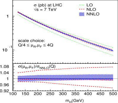
The past couple of years has seen several new NNLO calculations and they can roughly be divided into two classes: one class is that where NNLO delivers its promise of high precision, for example the inclusive calculation of vector-boson fusion Higgs-production [42] or the differential calculation of WH production [43]. The former is shown in Fig. 3 and, for once, the convergence is just as one would expect with a coupling $\sim 0.1$.

Figure 3: Recent NNLO predictions for inclusive vector-boson fusion [42] (left) and differential $\gamma\gamma$ production [44] (right).

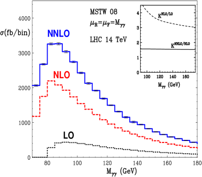
A second class of processes has more sobering results: Fig. 3 (right) shows the recent NNLO $\gamma\gamma$ [44] prediction where one sees $50\%$ corrections in going from NLO to NNLO. Yet another case where NNLO appears to face difficulties and that has seen extensive discussion is for the prediction of the efficiency of jet vetoes in Higgs production [45].

Various physics mechanisms can lead to this poor behaviour of the perturbative series: Sudakov logarithms when one puts excessively stringent cuts on the final state; threshold logarithms when one is limited by the available partonic centre of mass energy; and the appearance of partonic scattering channels at NLO or NNLO that weren’t possible at lower order (e.g. $qq\to qq\gamma\gamma$). Still despite progress on individual aspects (e.g. Higgs Sudakov boson [46, 47] and jet [48, 49, 50, 51] $p_{t}$ resummations, Higgs threshold resummations [52, 53, 54], or the combination of processes with different multiplicities [55]), one cannot help but wonder whether with more insight we might not obtain predictions that just systematically converge better.

I cannot close this section without mentioning a result that appeared only after my talk, the NNLO corrections to $q\bar{q}\to t\bar{t}$ [56]. It’s the first time that a NNLO calculation appears for a process involving coloured particles in both initial and final states and as such is a groundbreaking achievement. It brings significantly improved precision, at the $3\%$ level (roughly a factor of $3$ improvement over NLO), to the prediction of the Tevatron $t\bar{t}$ cross section.

4.2 Rethinking searches

It can be tempting to say that if only we knew collider backgrounds better we would significantly improve the reach of a range of searches. But I believe it’s just as important to ask the question of whether using our understanding of QCD can help us to find better analysis techniques, techniques that improve signal-to-background ($S/B$) ratios (and sometimes also $S/\sqrt{B}$) and so reduce the impact of background uncertainties.

One example of this is in the search for $b\bar{b}$ decays of a light Higgs boson when produced in association with a W or Z. Long thought to be inaccessible due to huge backgrounds, this channel became possible again after the results of [57], which showed how to improve signal to background ratios by going to high $p_{t}$ (backgrounds drop faster than signal) and developing appropriate “boosted-Higgs” jet-substructure reconstruction methods. Since then, the idea of going to high $p_{t}$ has been adopted in [58, 59], though there are insufficient data so far to truly benefit from the new jet substructure methods. In parallel, this and other early work has spurred a whole new field of investigation into event-topologies with boosted tops, vector and Higgs bosons, and BSM particles, together with extensive further developments on the jet-substructure analysis techniques. Several reviews cover this progress in detail [60, 61, 62].

While “boosted-object” searches have garnered much of the attention recently, progress is also being made in better signal detection in other areas too: quark/gluon discrimination has recently seen a renewal of interest [63] and may have applications in many searches; and there is clearly scope for novel methods even in “standard” SUSY searches [64].

A general question that remains open here is whether such improvements will continue to come mainly from an intuitive understanding of QCD v. BSM differences, as has largely been the case so far, or whether there is a benefit to be had also from more quantitative, analytical insight into how signals and backgrounds differ.

5 Conclusions

Figure 4: The papers most frequently cited by the ATLAS and CMS collaborations (excluding citations to ATLAS and CMS), showing the fraction of ATLAS and CMS papers that refer to each one. The lists of ATLAS and CMS papers were taken from their respective websites and the citations data from INSPIRE.

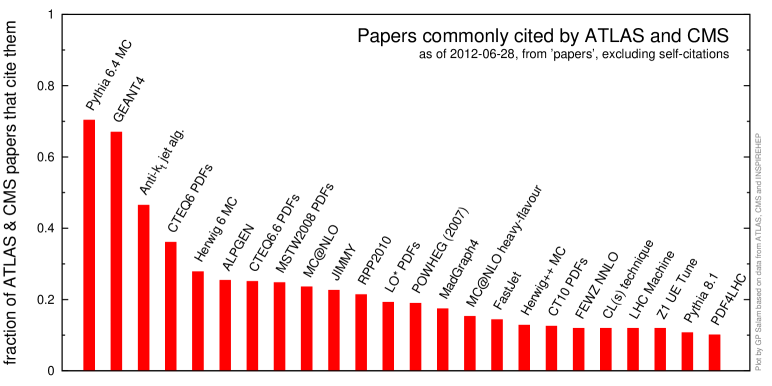
Many of the cutting-edge QCD research results discussed here have come with an initial focus on one or other specific class of search or application. It is interesting to look also at what the LHC experiments use across the board, on a day-to-day basis. Fig. 4 shows the papers most commonly referred to by ATLAS and CMS and, for each, the fraction of the collaborations’ articles that refer to them. Some aspects of this graph are unsurprising, such as the overwhelming role played by Pythia. Other aspects provide a reminder that such citations data should be interpreted with an abundance of caution: one can’t help but notice the position of the “LHC Machine” relative to Pythia. Still, it is striking that of the 24 articles shown (those cited by more than $10\%$ of the collaborations’ papers), 20 stem from the QCD community, a tribute to the key role being played by QCD at the LHC.