Vortex-Bright Soliton Dipoles: Bifurcations, Symmetry Breaking and Soliton Tunneling in a Vortex-Induced Double Well

Abstract

The emergence of vortex-bright soliton dipoles in two-component Bose-Einstein condensates through bifurcations from suitable eigenstates of the underlying linear system is examined. These dipoles can have their bright solitary structures be in phase (symmetric) or out of phase (anti-symmetric). The dynamical robustness of each of these two possibilities is considered and the out-of-phase case is found to exhibit an intriguing symmetry-breaking instability that can in turn lead to tunneling of the bright wavefunction between the two vortex “wells”. We interpret this phenomenon by virtue of a vortex-induced double well system, whose spontaneous symmetry breaking leads to asymmetric vortex-bright dipoles, in addition to the symmetric and anti-symmetric ones. The theoretical prediction of these states is corroborated by detailed numerical computations.

I Introduction

Within the booming field of Bose-Einstein condensation (BEC), the study of coherent nonlinear states has its own considerable history emergent ; revnonlin ; rab ; djf . The original explorations were in the setting of repulsive interatomic interactions, and especially so in the context of one-component settings, starting over a decade ago han1 ; nist ; dutton ; bpa . These works chiefly focused on the dark soliton i.e., the prototypical nonlinear state therein, yet they were considerably hampered by instability effects induced by the dimensionality of the system and/or the presence of thermal effects. Nevertheless, more recent efforts using a variety of techniques have been far more successful in generating robust (dark) solitary wave states. Such techniques include phase-imprinting/density engineering hamburg ; hambcol ; technion , matter-wave interference kip ; kip2 , or dragging localized defects through the BECs engels . The two-dimensional generalization of such (dark) states has as its prototype the vortex waveform, which became possible Matthews99 by using a phase-imprinting method between two hyperfine spin states of a ⁸⁷Rb BEC Williams99 . Subsequent efforts involved the stirring of the BECs Madison00 above a certain critical angular speed Recati01 ; Sinha01 ; corro ; Madison01 which, in turn, led to the production of few vortices Madison01 and even of very robust vortex lattices Raman . Other techniques including dragging obstacles through the BEC kett99 or the nonlinear interference of condensate fragments BPAPRL have been also used for the production of unit-charge vortices. Higher-charged vortex structures were produced S2Ket and their dynamical (in)stability has been examined.

All of the above explorations were developed in the context of one-component BECs. Yet, solitary wave states also exist in multi-component BEC settings. In that context, of growing interest within the past few years has been the study of dark-bright (DB) solitons that are supported in two-component BA and even spinor DDB condensates. These states can be thought of as “symbiotic”, in that the bright second component could not be sustained in the absence of the trapping dark first component. Robust such states were first observed in the experiment of Ref. hamburg by means of a phase-imprinting method.

This, in turn, has led to experimental studies of numerous features of these multi-component waves including the realization of DB soliton trains engels1 , DB soliton oscillations and interactions engels2 ; engels4 , as well as the possibility to create dark-dark breathing counterparts of these states (and multi-wave generalizations thereof) engels3 ; engels5 . In two dimensions, generalizations of these states have been proposed in the form of vortex-bright (VB) solitons, which were introduced about a decade ago (see e.g. skryabin and references therein) and were recently further explored in the work of kody .

It is with the VB waveforms that we will concern ourselves in the present study. Early experiments, such as the one of anderson , have illustrated the feasibility of realization of these states. Additionally, recent studies of dynamical phenomena in two-component condensates with considerable temporal and spatial resolution and control wieman ; mertes ; egorov suggest that the relevant coherent states can be explored further. Our aim here is to explore this potential beyond the level of a single vortex-bright soliton entity. In particular, recently in the one-component setting, we have examined the bifurcation of few-vortex clusters (see bifurcation and references therein), most notably the vortex dipole, but also the vortex tripole, quadrupole, vortex polygons and larger scale crystals stephan_physd . It is then natural to expect that similar bifurcations will arise in the two-component setting and, in fact, that the bright solitons that are “trapped” within the vortex states will potentially bear different relative phases (e.g. in phase or out of phase, as is the case with DB solitons in engels4 ). It is relevant to mention here that particular (in phase) realizations of such states have been very recently proposed as realizable by means of numerical dragging experiments in the immiscible regime of the pseudo-spinor system in gautam . The excitations resulting by dragging a laser beam through the two-component system had earlier been explored in the miscible regime in susanto .

The vortex-bright dipoles, consisting of a vortex pair of opposite circulation and a corresponding trapped bright soliton pair, will be the main theme herein. We will start by providing the background of the relevant model and theoretical setup, as well as a brief review of the properties of a single VB soliton in section II. Then, in section III, we will explain the different types of [in phase (IP), or out of phase (OOP)] VB dipoles that exist and will present their bifurcation from the (nonlinear) continuation of underlying linear states in the form of dark-bright soliton stripes. In section IV, we examine the stability of the VB dipoles and recognize an instability of the OOP states and its symmetry breaking and tunneling implications. These are then theoretically explained in the form of an effective double well theory (as induced by the vortices on the bright components) and its symmetry breaking bifurcations, which gives rise to rather unexpected genuinely asymmetric VB dipole states. We summarize our findings in section V, where we also present some conclusions and possible directions for future studies.

We should mention in passing that although our principal focus herein will stem from BEC and atomic physics considerations, relevant topics and ideas are, in principle, relevant for nonlinear optics as well. In particular, structures such as dark solitons kivshar_luther and vortices yuripismen ; dragomir have been extensively studied in the latter field. In fact, DB-soliton states were also first observed in optics experiments, where they were created in photorefractive crystals seg1 , while their interactions were discussed in Ref. seg2 . It is thus natural to expect that the combination of multi-component and multi-dimensional settings therein would also yield further potential for the realizability and observation of the coherent structures analyzed in the present work.

II Model Setup

Our starting point will be the setting of quasi two-dimensional repulsive binary BECs, whose mean field description is given by the following set of equations:

$$i\partial_{t}\psi_{1}(x,y,t) =\left[-\frac{1}{2}(\partial_{x}^{2}+\partial_{y}^{2})+V(x,y)+g_{1}|\psi_{1}|^{2}+\sigma_{12}|\psi_{2}|^{2}\right]\psi_{1}(x,y,t)$$

$$i\partial_{t}\psi_{2}(x,y,t) =\left[-\frac{1}{2}(\partial_{x}^{2}+\partial_{y}^{2})+V(x,y)+g_{2}|\psi_{2}|^{2}+\sigma_{12}|\psi_{1}|^{2}\right]\psi_{2}(x,y,t)\text{.}$$ (1)

This coupled dimensionless set of Gross-Pitaevskii (GP) equations describes the time evolution of the two components’ order parameters $\psi_{j}$, $j\in\{1,2\}$. Time, length, energy and densities $|\psi_{j}|^{2}$ are measured in units of $\omega_{z}^{-1}$, $a_{z}$, $\hbar\omega_{z}$ and $(2\sqrt{2\pi}|a_{12}|a_{z})^{-1}$, respectively; $\omega_{z}$ and $a_{z}$ denote the oscillator frequency and length in the frozen $z$-direction, while $a_{11}$, $a_{22}$ and $a_{12}$ refer to the intra- and intercomponent scattering lengths. In the resulting dimensionless form of the equation, the coupling constants are $g_{j}=a_{jj}/|a_{12}|$, and $\sigma_{12}$ denotes the sign of $a_{12}$. From here, all equations will be presented in dimensionless units and all the quantities which are plotted are dimensionless as well.

In the following, we will analyze the relevant case of binary condensates composed of ⁸⁷Rb atoms in the two spin states ($F=1$, $m_{F}=-1$) and ($F=2$, $m_{F}=1$), leading to dimensionless coupling constants of approximately $g_{1}=1.03$, $g_{2}=0.97$, $\sigma_{12}=+1$ emergent , and we will exclusively consider isotropic harmonic potentials $V(x,y)=\Omega^{2}(x^{2}+y^{2})/2\equiv\Omega^{2}r^{2}/2$, where $\Omega=\omega_{r}/\omega_{z}$ denotes the ratio of the in-plane and out-of-plane oscillator frequencies and is fixed to $0.2$. This trap strength is only selected for reasons of computational convenience (and experimental realizability), but the phenomenology presented below will not depend in any critical way on this selection for quasi-two-dimensional BECs. Stationary solutions are obtained by factorizing $\psi_{j}(x,y,t)=\exp(-i\mu_{j}t)\phi_{j}(x,y)$, $j\in\{1,2\}$, where $\mu_{1}$ and $\mu_{2}$ are the two components’ chemical potentials.

The prototypical stationary solution of Eq. (1) that will be the building block for our considerations is the single vortex-bright soliton state, whose density and phase profiles are shown in Fig. 1. For such a state, the first component supports a vortex, which acts as an effective potential well for the second component (of course, the alternative arrangement also exists where the role of the components is interchanged). However, we will focus solely on the former case due to its unconditional stability; as discussed e.g. in skryabin ; kody , in the case where the components are interchanged, parametric regimes of instabilities may arise.

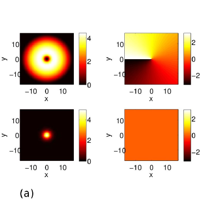
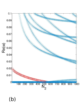
Figure 1: (Color online) (a) Numerically calculated vortex-bright soliton solution to the two-component Gross-Pitaevskii equation obtained for $N_{1}=2000$ and $N_{2}=100$. The density (left) and the phase (right) of the two components is shown. All the other state profiles shown throughout the present work will use the same color coding, with the colorbars ranging from zero to maximum density and $-\pi$ to $+\pi$, respectively. (b) BdG spectrum of the vortex-bright soliton for $\mu_{1}=5.2$ as a function of $N_{2}$. Just the real part of the eigenfrequencies $\omega$ is shown, as the imaginary part is found to be identically zero for all values of $N_{2}$. Negative energy modes are indicated by darker square markers (red in the online version).

The linear stability (so-called Bogolyubov-de Gennes or BdG) analysis is employed in order to consider the fate of small amplitude perturbations and the potential robustness of the solutions. This consists of imposing a perturbation to the stationary solutions $\phi_{j}$ above in the form:

$$\psi_{1}(x,y,t) = \exp(-i\mu_{1}t)\left\{\phi_{1}(x,y)+\varepsilon\left[a(x,y)e^{i\omega t}+b^{\ast}(x,y)e^{-i\omega^{\ast}t}\right]\right\},$$ (2)

$$\psi_{2}(x,y,t) = \exp(-i\mu_{2}t)\left\{\phi_{2}(x,y)+\varepsilon\left[c(x,y)e^{i\omega t}+d^{\ast}(x,y)e^{-i\omega^{\ast}t}\right]\right\}.$$ (3)

This leads at $\mathcal{O}(\varepsilon)$ (where $\varepsilon$ is a formal small parameter) to an eigenvalue problem for the (in principle, complex) frequency of excitations $\omega$ and the corresponding eigenvector $[a(x,y),b(x,y),c(x,y),d(x,y)]^{T}$. Further details about the mathematical structure of the BdG two-component problem can be found in skryabin . For our purposes, it suffices to note that the Hamiltonian structure of the resulting eigenvalue problem enforces that if $\omega$ is an eigenfrequency so are $\omega^{\ast}$, $-\omega$ and $-\omega^{\ast}$. Hence, if eigenfrequencies with Im$(\omega)\neq 0$ exist, then the solution is deemed to be dynamically unstable.

A prototypical example of the BdG spectrum of a VB solitary wave is provided in Fig. 1(a). In this example, the spectrum is offered as a function of the (rescaled) number of atoms in the bright soliton component $N_{2}=\int\text{d}x\text{d}y|\psi_{2}|^{2}$, while the chemical potential of the dark (vortex) component stays fixed at $\mu_{1}=5.2$. One important observation to make here is that there is a single negative energy mode skryabin in the spectrum of the vortex for small (or vanishing) $N_{2}$. This mode is illustrated by the square markers (which are red in the online version) in the relevant panel and is well-known to correspond to the precession of the vortex within the parabolic trap (see e.g. bifurcation and references therein). However, it is noteworthy that this mode decreases in frequency due to the presence of the bright component and ultimately crosses the zero frequency point. Yet, this crossing does not produce an instability; the relevant eigenfrequency pair remains real but now the energy of the mode is positive signaling the transition of the vortex state from a saddle in the energy landscape into a local minimum thereof (this is a setting analogous to what is observed for a vortex in the presence of rotation; see e.g. the relevant discussion of castin ). It is important to note that this observation is in agreement with the results described in anderson , where it was observed that filled vortex cores exhibit slower precessions, and thus a decrease of the precession frequency is expected. It is relevant to note that similar observations have also been obtained in the case of dark-bright solitons, originally through the theoretical analysis of BA and have been experimentally confirmed in the work of engels2 .

III Vortex-Bright Soliton Dipole States

Using the above fundamental building blocks, namely the single VB solitons, we now look for bound states containing multiple such entities. In the same spirit as in the work of bifurcation (see also e.g. komineas and references therein), the prototypical relevant bound state is the VB dipole. We have been able to identify two such states, which are both shown in Fig. 2 for $N_{1}=70$ and $N_{2}=20$. In both cases the first component contains two vortices located symmetrically with respect to the trap center, which are filled by the second component. The difference between the two dipoles is evident in the phase profile: the two bright solitons filling the vortex cores can have either the same phase, or there may be a phase difference of $\pi$ between them.

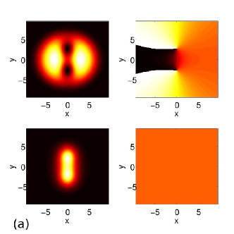
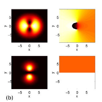
Figure 2: (Color online) (a) Density (first column) and phase (second column) of an in-phase vortex-bright dipole. (b) Density (third column) and phase (fourth column) of the out-of-phase vortex-bright dipole. Both examples are for $N_{1}=70$ and $N_{2}=20$.

The emergence of the dipole state branches can be thought of in terms of a bifurcation picture in an equivalent way to the one described for one-component BECs in bifurcation . The two possible dipole branches, distinguished from the presence or absence of the phase jump of $\pi$ in the bright component, arise at critical values of $N_{1}$ from two states, which can be regarded as generalizations of the dark soliton stripe observed in one-component condensates djf . The density and phase profiles of these two solitonic states are shown in the top panels of Figs. 3(a) and  3(b), where it is evident that the two states are again distinguished by the presence or absence of a $\pi$-phase jump in the bright component.

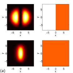
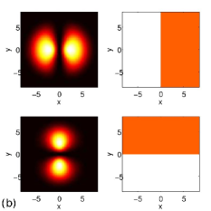
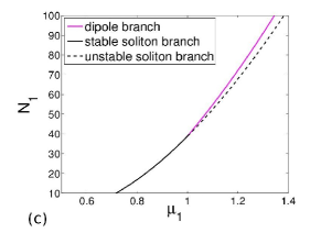
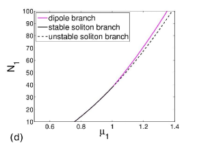
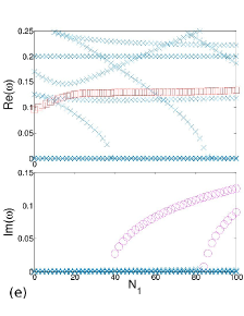
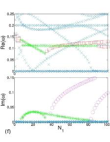
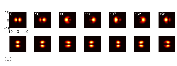
Figure 3: (Color online) (a) Density and phase of the in-phase dark-bright soliton stripe, $N_{1}=38$, $N_{2}=20$. (b) Density and phase of the out-of-phase dark-bright soliton stripe, $N_{1}=38$, $N_{2}=20$. In the second row we see the bifurcation of the IP and OOP ((c) and (d), respectively) vortex-bright soliton dipoles branch from the corresponding parent states (whose density and phase profiles are depicted in (a) and (b)). The third row’s panels contain the BdG analysis of the parent states (in (e) and (f) we see the IP and the OOP case, respectively) of the top panels, illustrating the instability (through an imaginary eigenfrequency, signaled by pink circle markers) that is induced by the emergence of the vortex-bright dipoles. In addition, for the out-of-phase case, the lines formed by “$\ast$“ (green in the online version) markers correspond to the existence of oscillatory instabilities through complex eigenfrequency quartets. In this case there are two anomalous modes (depicted by red square markers), while there is only one such for the in phase stripe. (g) Time evolution of the out-of-phase dark-bright soliton stripe after being perturbed with the eigenvector of one of the oscillatorily unstable modes at $N_{1}=N_{2}=20$. The top and bottom lines depict the density profiles of the dark and bright component, respectively, evaluated at seven moments of the simulated evolution. The elapsed (dimensionless) time is indicated in the panels’ upper left corners.

In the first case of the IP VB dipole, the parent state can be seen to consist of a dark soliton stripe in the first component accompanied by a bright stripe in the second component, which is trapped inside the dark stripe. In the notation of the corresponding linear limit of the two single-particle Hamiltonians, the relevant state of the first component is the $|1,0\rangle$ state (i.e., the first excited state in the x-direction) while that of the second component is the $|0,0\rangle$ ground state of the latter. More generally, the symbolism $|m,n\rangle$ is used to denote the states $H_{m}(\sqrt{\Omega}x)H_{n}(\sqrt{\Omega}y)e^{-\Omega r^{2}/2}$ where $H_{m}$ stands for the m-th Hermite polynomial and normalization constants have been omitted. These are stationary states of the underlying linear problem with eigenvalue $\mu=\Omega(m+n+1)$, from which the soliton stripe solutions arise in the presence of the effective nonlinearity induced by interatomic interactions. It is the nonlinearity and immiscibility of the two components that leads to the $|0,0\rangle$ state of the second component being elongated (as opposed to circularly symmetric) in the dark-bright stripe of Fig. 3(a). Corresponding states in a ring (as well as in diagonal stripes) form have recently been addressed in jan2 . In the case of the OOP VB dipole, shown in Fig. 3(b), the parent state is the $|1,0\rangle$ of the first component coupled to the $|0,1\rangle$ of the second component.

While the bright component remains roughly invariant as the transition point is crossed, the dark component develops two singular points in the phase corresponding to the density vanishings and the opposite circulation characteristic of a vortex dipole bifurcation . The relevant bifurcations occur approximately at the same critical $N_{1}$ ($N_{1}^{cr}\approx 40$, with $N_{2}$ fixed at $20$). This is explicitly depicted in Figs. 3(c) and  3(d) for the two different “stripe” states, where the $N_{1}(\mu_{1})$ bifurcation diagrams are shown. These approximately equal critical values of $N_{1}$ can, arguably, be expected due to the small number of particles of the second component, a statement which becomes exact in the limit of $N_{2}\rightarrow 0$.

The BdG analysis of the two stripe states is shown in Figs. 3(e) and 3(f) and allows to relate the emergence of the dipole state to the changing of stability of the parental branch (the IP and OOP solitonic states).

From the BdG spectra, in fact, one observes the emergence of an imaginary eigenfrequency pair for $N_{1}^{cr}\approx 40$, which is the value of $N_{1}$ at which the bifurcation actually occurs. Imaginary modes are here depicted by circle (pink in the online version) markers. The ”$\ast$” (green in the online version) markers are used to identify complex modes which are related to oscillatory instabilities, resulting from the collision of positive energy modes (associated with the “background” on top of which the coherent solitonic structures exist) with negative energy modes that are associated with the solitonic structures (and the fact that they are not ground states of the system). For detailed discussions of the such instabilities and their origin, see  emergent ,  revnonlin and  skryabin .

The complex nature of such eigenvalues (or eigenfrequencies) leads to a part associated with oscillation (connected to the real part of such eigenfrequencies) and a part associated with growth (the imaginary part of such eigenfrequencies). Hence, what one should expect upon perturbation of such eigenmodes is an oscillatory growth that should lead to a destabilization and eventual destruction of the relevant solitonic structures (of Figs. 3(a) and 3(b)). This effect is evident in Fig. 3(g), where the propagation of the OOP soliton for $N_{1}=20$ and $N_{2}=20$, after the excitation of one of the two complex eigenmodes, is shown. Exciting the other mode, one obtains an equivalent evolution of the system, by interchanging the roles of the two components: the oscillation is observed in the other component. As is evident from the BdG spectra, here an oscillatory instability exists for the OOP solitonic state but not for the IP solitonic state. In this context, let us point out that the IP stripe bears only one negative energy mode, while a second such anomalous mode is present in the OOP state’s spectrum. As a result, the IP configuration is less prone to oscillatory instabilities emerging from collisions of anomalous and background modes than the OOP one. The presence of one anomalous mode for the IP state and of two such modes for the OOP state is intuitively expected by the out-of-phase or excited state nature that the former bears only in the first component, while the latter has that type of structure in both components. I.e., in the second component, the former configuration features a ground state, symmetric waveform, while the latter has an anti-symmetric first excited state waveform. This type of characteristics will be of critical relevance to the considerations that follow below, regarding tunneling effects and symmetry-breaking bifurcations.

IV Tunneling Dynamics and Symmetry-Breaking Bifurcations

Let us now come back to the vortex-bright soliton dipoles and especially their dynamical stability through the BdG analysis. The in-phase VB dipole appears to be stable for arbitrary values of $N_{1}$ and $N_{2}$, while the out-of-phase VB dipole shows purely imaginary modes arising at certain values of $N_{1}$ and $N_{2}$ (when the state is scanned over $N_{1}$ or $N_{2}$, respectively), see Fig. 4(a). Exciting this unstable mode for the OOP dipole with $N_{1}=220$ and $N_{2}=1$ by adding some white noise and letting the perturbed states propagate in time, the evolution shown in Fig. 4(b) is obtained.

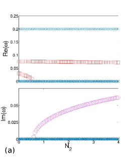
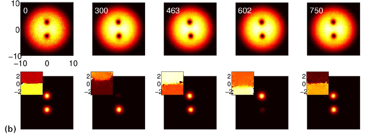
Figure 4: (Color online) (a) BdG spectrum of an out-of-phase vortex-bright soliton dipole for $N_{1}=220$ as a function of $N_{2}$. According to our convention, pink circle markers are related to unstable imaginary modes, while red square markers identify anomalous modes. (b) Time propagation of the same state at $N_{1}=220$ and $N_{2}=1$. Again, the top and bottom lines depict the density profiles of the dark and bright component, respectively. At the upper left corners of the pictures of the second row the phase of the bright component, evaluated at the same time steps as the density profiles, is shown. The substantial addition of white noise (that seeds the instability) can be seen in the pixelization of the corresponding dynamical panels.

The time evolution of the density profiles shows the size of one of the bright solitons increasing while the other one is getting smaller, then the opposite situation is observed and this trend with enlarging and shrinking bright solitons is repeating in the course of the propagation. After an initial transient phase during which the bright component’s asymmetry builds up (first to second time step shown in Fig. 4(b)), we find periodic oscillations. This observed time evolution has an immediate physical interpretation as concerns the bright component. A fraction of the corresponding particles within the second component move from one vortex core to the other during the time propagation of the system. This can be explained by considering the dark component’s density as acting in the form of an effective potential for particles of the bright one. I.e., the particles of the second component can be considered as tunneling within the vortex-induced (i.e., formed by the vortex cores) double well potential. Within this very potential, this suggests the possibility of a spontaneous symmetry breaking bifurcation, as responsible for the observed phenomenology.

In order to validate this assumption, we consider the analytical model, developed in symmetry , based on a two-mode expansion, which is used to determine stationary states and to study the symmetry-breaking bifurcations occuring in one-dimensional, single-component repulsive BECs confined in double-well potentials. The model predicts that for a two-mode decomposition of the equation involving a symmetric ground state and an anti-symmetric first excited state, there exists a symmetry breaking bifurcation both for attractive and for repulsive interactions. The bifurcation emerges from (and destabilizes) the anti-symmetric, first-excited state in our repulsive interaction case (while it stems from and destabilizes the symmetric ground state in the attractive interaction case). This is consonant with the principal observation above of the generic stability of the IP VB, which has a symmetric second component and the symmetry breaking associated destabilization of the OOP VB with the anti-symmetric second component.

The key quantitative observation now is that if we freeze the first component (assuming that it forms the vortex-core double well potential), then the theory of symmetry can be applied directly but for the effective double well potential in the form $V_{\text{eff}}(x,y)=V(x,y)+|\psi_{1}(x,y)|^{2}$, where $V(x,y)$ is the trapping harmonic potential. The equation for the second component can then be rewritten as

$$i\partial_{t}\psi_{2}(x,y,t)=\left[-\frac{1}{2}\Delta_{2D}+V_{\text{eff}}(x,y)+g_{2}|\psi_{2}|^{2}\right]\psi_{2}(x,y,t),$$ (4)

which upon the rescaling $\tilde{\psi}_{2}(x,y)=\sqrt{g_{2}}\psi_{2}(x,y)$ leads to a standard single-component (two-dimensional) double well setting. It should be noted that the potential of the double well clearly depends on $N_{1}$ (through its dependence on $|\psi_{1}(x,y)|^{2}$). For each $N_{1}$ (in multiples of $5$) in the interval $[0,300]$ the density profile of the dark component of the VB dipole state with $N_{2}=0$ has been utilized (to form the corresponding effective potential). For each considered value of $N_{1}$, one can diagonalize the obtained Hamiltonian $H=-\frac{1}{2}\Delta_{2D}+V_{\text{eff}}$, and keep the two lowest energy eigenstates, namely the symmetric ground state and the anti-symmetric first excited state of the single particle operator with the effective potential. These, denoted hereafter as $u_{0}(x,y)$ and $u_{1}(x,y)$, will be used for the two mode reduction in the spirit of symmetry .

The fundamental analytical prediction of the two-mode approximation is that as $N_{2}$ (and $\mu_{2}$) is increased, a critical point will be reached, given by

$$N_{2cr}=\frac{\Delta\omega}{(3B-A_{1})g_{2}},$$ (5)

whereafter the anti-symmetric branch (interpreted here as the OOP VB dipole) will become unstable. Past this critical point, an asymmetric branch (i.e., an asymmetric VB dipole) should emerge as a stable configuration. In the expression of Eq. (5) $A_{1}=\int u_{1}^{4}\text{d}x\text{d}y$ and $B=\int u_{0}^{2}u_{1}^{2}\text{d}x\text{d}y$ are overlap integrals of the two lowest energy eigenstates of the linear Schrödinger problem and $\Delta\omega=\omega_{1}-\omega_{0}$, where $\omega_{0}$ and $\omega_{1}$ are the energy eigenvalues corresponding to $u_{0}$ and $u_{1}$. The presence of the factor $g_{2}$ in the denominator ensures consistency with the scaling of $\psi_{2}$ discussed above.

The critical chemical potential is calculated from the particle number by making use of the expression $\mu_{2cr}=\omega_{0}+3BN_{2cr}$ symmetry .

Repeating this procedure for each considered $N_{1}$, we get the critical values of $\mu_{2}$, which are compared with the numerically obtained data; see Fig. 5(a). These latter are obtained by making a scan within a suitable interval of $N_{2}$ of the OOP VB dipole, and then performing the BdG analysis of the resulting branch of solutions. In the ensuing BdG spectrum, the bifurcation point can be identified as the onset of instability of the anti-symmetric VB dipole. For a relevant example, see again Fig. 4(a), for the scan obtained for $N_{1}=220$, where we can see the imaginary mode emerging at $N_{2}\approx 0.6$ (generally, the relevant critical values $N_{2}^{cr}$ are of order unity). At this critical value of $N_{2}$, for which the antisymmetric dipole becomes unstable (or, equivalently, at the corresponding critical value of $\mu_{2}$), we expect the bifurcation of a stable asymmetric state, which has been actually verified, as will be shown below.

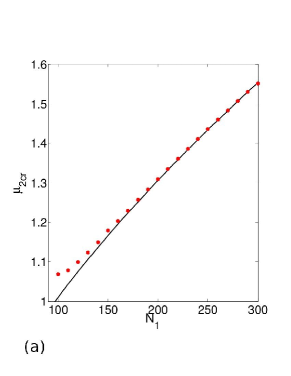
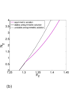
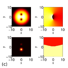
Figure 5: (Color online) (a) The critical points for the bifurcations of asymmetric states from the OOP dipole ($\mu_{2cr}$ for different values of $N_{1}$) are depicted by red circle points and are compared to the corresponding values of the theoretical two-mode prediction (solid black line). (b) The bifurcation diagram demonstrates the existence of an asymmetric vortex-bright dipole, as bifurcating from the out-of-phase one. (c) Example of density and phase profiles of such a symmetry-broken state.

From Fig. 5(a) it is evident that the agreement between analytical predictions and numerical results is very good for what concerns $\mu_{2cr}$ for $N_{1}\gtrsim 120$. For lower values of $N_{1}$ numerics and analytical predictions start to be in disagreement with each other and this has the following explanation: by decreasing $N_{1}$, the height of barrier between the two wells forming the effective potential $V_{\text{eff}}(x,y)=V(x,y)+|\psi_{1}(x,y)|^{2}$, is also decreased. Thus, for low $N_{1}$, the density $|\psi_{1}(x,y)|^{2}$ provides a much lower contribution to the potential, and the effect of the harmonic trap is much more appreciable. This influences the form of the energy spectrum: the gap separating the almost equal lowest energy eigenvalues $\omega_{0}$ and $\omega_{1}$ from the larger eigenvalues $\omega_{2}$, $\omega_{3}$…, which is typically large for a high barrier, if the latter is lowered becomes smaller and smaller, until the spectrum of the harmonic oscillator, formed by equidistant eigenvalues, is reached. But, if this is the case, the two-mode approximation that one makes by projecting the problem on the eigenmodes $u_{0}$ and $u_{1}$ fails as the contribution of the other eigenstates cannot be neglected anymore.

Furthermore, another intuitive argument can be provided to explain the disagreement between predicted and numerical results observed with lowering $N_{1}$: as was already said, the effective potential $V_{\text{eff}}(x,y)=V(x,y)+|\psi_{1}(x,y)|^{2}$ has been calculated deriving the term $|\psi_{1}(x,y)|^{2}$ from the density profile of the dark component of the VB dipole state with $N_{2}=0$ and is considered to be fixed in the whole calculation. Our model looks for the bifurcation to occur at a finite value of $N_{2}$, but neglects that, for this value, in the actual physical system, the density profile for the dark component is different from the one with $N_{2}=0$. Thus, in doing this approximation, we do not take into account the effect of the second component on the first due to the interaction between them. Considering $V_{\text{eff}}$ independent of $N_{2}$ is expected to be valid if $N_{1}$ is large enough, as the dark component will then have a robust configuration with respect to variations due to the intercomponent interaction. But, decreasing $N_{1}$, varying $N_{2}$ will start to influence both components in a sensitive way and, in particular, an evident variation of the density profile of the dark component is expected. Therefore, for low $N_{1}$, the assumption that $|\psi_{1}(x,y)|^{2}$ is independent of $N_{2}$ is no longer appropriate and the model described above cannot be expected to be valid anymore. Therefore, in Fig. 5(a), values of $N_{1}$ smaller than $100$ are not taken into account.

Let us now come back to the expected bifurcation from the anti-symmetric branch, once its destabilization occurs, towards an asymmetric VB dipole solution. Indeed, an example of this bifurcation has been illustrated in Fig. 5(b). Note that this diagram is the direct analog of Fig. 4 in symmetry , where symmetry-breaking bifurcations in a one-dimensional static double well were studied. Fig. 5(c) illustrates a prototypical example of the daughter state in the form of an asymmetric vortex-bright dipole.

The robustness of an asymmetric VB dipole of the type shown in Fig. 5(c), combined with the Hamiltonian dynamics of the system, is what gives rise to the tunneling observations of Fig. 4(b). Naturally, there are two such asymmetric states, depending on which vortex-induced well picks up part of the bright mass of the other, justifying the pitchfork character of the bifurcation. The BdG spectrum of the asymmetric state (not shown here) reveals the complete stability of the latter, in accordance with the expectations from the above bifurcation theoretic arguments.

Let us in the following further explore the analogy between the bright component effectively trapped by the dark vortex dipole and a single species BEC in an external double well potential. The possible types of dynamics in such a double well setting (sometimes called a bosonic Josephson junction) have attracted a lot of attention and have been studied both theoretically and experimentally in great detail, see e.g. oberthaler and references therein. The existence of asymmetric (“self-trapped”) solutions in such a setting was first studied in BJJ1 ; BJJ . We have performed a number of numerical simulations to show that starting from suitable initial conditions for the bright component in the VB dipole, all types of characteristic dynamics in such a bosonic Josephson junction can be recovered. In particular, in the parameter regime where asymmetric states have bifurcated from the antisymmetric solution, three profoundly different types of dynamics are possible, namely: oscillations around the self-trapped, asymmetric configurations, tunneling oscillations between the two wells with a mean relative phase of 0 (“plasma oscillations” around the in-phase fixed point) and such with a mean relative phase of $\pi$, the so-called “$\pi$ oscillations” around the $z$-symmetric out-of-phase fixed point, see e.g. oberthaler . These three types of trajectories are most easily distinguished in phase space of the conjugate variables $(z,\phi)$, where $z$ denotes the population imbalance between the two wells and $\phi$ is the corresponding phase difference. More formally, these two quantities can be extracted from the full wavefunction within the two-mode approximation introduced above, taking into account only the ground and first excited states of the double well. Starting from the known lowest symmetric and antisymmetric eigenfunctions $u_{0}$ and $u_{1}$, modes which are localized in one of the wells can be formed, namely $u_{D,U}=(u_{0}\pm u_{1})/\sqrt{2}$. Expanding the full wavefunction in this basis, $\psi_{2}=\sqrt{\rho_{U}}\exp(i\phi_{U})u_{U}+\sqrt{\rho_{D}}\exp(i\phi_{D})u_{D}$, where both $\rho_{U,D}$ and $\phi_{U,D}$ are real, the phase space variables are calculated as $\phi=\phi_{U}-\phi_{D}$, $z=(\rho_{U}-\rho_{D})/(\rho_{U}+\rho_{D})$. A number of different trajectories of the bright component in the vortex-induced double well, presented in terms of these $(z,\phi)$ variables, are shown in Fig. 6(a) for parameter values $N_{1}=220$, $N_{2}=1$. In Fig. 6(b), the $z(t)$ dependence for three different trajectories is shown.

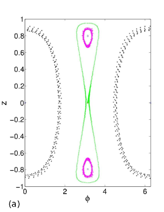
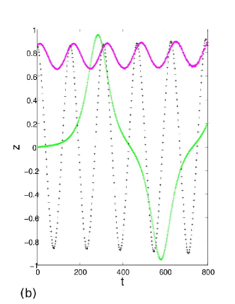
Figure 6: (Color online) (a) The three types of trajectories of the bright component in the vortex-induced double well at $N_{1}=220$, $N_{2}=1$. The conjugate variables $z$, $\phi$ denote the population imbalance and phase difference between the two wells, respectively. All three types of expected trajectories can be seen to exist: oscillations around the asymmetric, stable fixed points (magenta, $\ast$ markers), plasma oscillations between the wells around an average phase of 0 (black, $+$ markers) and $\pi$ oscillations, i.e. tunneling oscillations with an average phase difference of $\pi$ between the two vortex cores (green, $\times$ markers, same data as in Fig. 4). The plot also shows the in-phase, out-of-phase and asymmetric fixed points of the system. (b) $z(t)$ dependence for the three trajectories, presented in the same color-markers code.

There is full agreement of this phase portrait with the one obtained for a single species bosonic Josephson junction e.g. in oberthaler , indicating that for the small populations in the bright component we are considering here, the approximation of “freezing” the dark component into an effective double well potential is a very good one. Finally, Fig. 7 collects density and phase profiles of the two remaining trajectories included in the phase portrait, namely the one revolving around one of the self-trapped, asymmetric states (Fig. 7(a)) and a “plasma oscillation” (Fig. 7(b)) around the symmetric, in-phase configuration (while the “$\pi$ oscillation” around the antisymmetric fixed point was already shown in Fig. 4(b)).

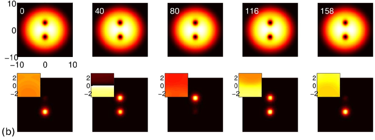
Figure 7: (Color online) Simulated density profiles of both components and phase profiles of the bright component during an oscillation around one of the self-trapped states (a) and during a plasma oscillation (b), same data as included in the phase portrait Fig. 6.

So far, we have concentrated this section’s discussion of the tunneling dynamics on the regime of small $N_{2}$, close to the linear limit of the effective Hamiltonian introduced by assuming the dark component to be frozen. While this is essential for the simplified semi-analytical model introduced above to make the connection to symmetry-breaking in a double well potential, we have found direct numerical evidence that the out-of-phase VB dipole is unstable towards tunneling dynamics in the bright component even in parameter regimes where $N_{2}$ is considerably larger, see Fig. 8 for an example. In this case the larger population of the bright component now leads to a stronger back-coupling to the dark component. In particular, it can now be clearly observed that the vortex cores forming the dipole in the dark component change size following the trend of the bright solitons filling them. While in Fig. 4(b) the tunneling oscillations, past the initial transient of asymmetry build-up, directly turn periodic, this is no longer the case here. Instead, in the run shown in Fig. 8, the bright component first almost completely tunnels to the lower well, but then oscillates between this asymmetric and a more symmetric occupation of the two wells (see the first four timesteps shown). Only after that, a majority of bright component atoms enters the upper well (second to last timestep), and then directly oscillates back to approximately equal occupation of the vortex cores (last timestep). The conclusion of this first period is followed by a series of nearly equal period similar oscillation steps.

Figure 8: (Color online) Time propagation of an out-of-phase vortex-bright soliton dipole, perturbed with white noise at $N_{1}=390$ and $N_{2}=50$.

Another relevant difference to Fig. 4(b) is that the tunneling dynamics is accompanied by a rotational motion of the vortices, while for smaller $N_{2}$ the dipole essentially stayed aligned along the trap’s axis during the propagation. This may be taken as a hint that for a larger $N_{2}/N_{1}$ ratio the interspecies interaction may induce a coupling between the unstable tunneling-type mode of the bright component and the precessional degrees of freedom of the vortices in the dark component.

V Conclusions and Future Challenges

In the present work, we have revisited the vortex-bright solitary wave states and have illustrated their prototypical generalization to vortex-bright soliton dipoles. This is a first step towards the realization of two-component clusters of such entities. In the process, we have explored a number of interesting features. Firstly, even a single vortex-bright soliton was found to exhibit a transition from a saddle point in the energy to a local minimum, as its bright component becomes more significant. Secondly, two types of VB dipoles were identified, in analogy with their dark-bright one-dimensional counterparts. The first of them had the bright pulses (trapped inside the vortex cores) be in phase, while the other one had them as out of phase. We have identified the bifurcation of these states, as stemming from the corresponding dark-bright stripe states, one of which has the bright second component in phase (stemming from the ground symmetric state) and one of which has it out of phase (stemming from the first excited anti-symmetric state). Subsequently, the dynamical stability of the daughter VB dipole states emerging from these bifurcations was quantified. It was found that the in-phase one is generically stable, while the out of phase structure suffers an exponential instability (past a relevant critical point). The latter gave rise to tunneling dynamics and spontaneous symmetry breaking manifestations. This phenomenology was understood on the basis of an effective double well model, where the vortex cores played the role of the wells and led to asymmetric VB dipoles.

This study paves the way for a more detailed understanding of multi-component structures. One of the key items that remain open concerns the effective description of such states. In particular, it is remarkable that these states have both a solitonic character through their bright component and a vortex character through their dark one. It is then particularly interesting to examine how the effective equations characterizing the interactions of such entities look and what the corresponding interplay is between the vortex and the solitonic character. Another natural direction concerns generalizing the ideas presented herein to a setting with more vortex-bright dipoles e.g. three such, which might naturally be observable in two-component generalizations of the experiments of bagnato . In fact, careful inspection of the figures presented herein (see e.g. the second pair of imaginary eigenfrequencies stemming from the stripe states’ BdG analysis in the bottom panel of Fig.  3) already suggests the bifurcation of such states. Furthermore, extending the present considerations to three-dimensions and towards a more detailed understanding of bound states of vortex rings pantoflas (and two-component generalization thereof) would also constitute an important theme for future explorations. Such studies are presently in progress and will be reported in future works.

References

- (1) P. G. Kevrekidis, D. J. Frantzeskakis, and R. Carretero-González, Emergent Nonlinear Phenomena in Bose-Einstein Condensates: Theory and Experiment (Springer-Verlag, Heidelberg, 2008).
- (2) R. Carretero-González, D. J. Frantzeskakis, and P. G. Kevrekidis, Nonlinearity 21, R139 (2008).
- (3) F. Kh. Abdullaev, A. Gammal, A. M. Kamchatnov, and L. Tomio, Int. J. Mod. Phys. B 19, 3415 (2005).
- (4) D. J. Frantzeskakis, J. Phys. A: Math. Theor. 43, 213001 (2010).
- (5) S. Burger, K. Bongs, S. Dettmer, W. Ertmer, K. Sengstock, A. Sanpera, G. V. Shlyapnikov, and M. Lewenstein, Phys. Rev. Lett. 83, 5198 (1999).
- (6) J. Denschlag, J. E. Simsarian, D. L. Feder, C. W. Clark, L. A. Collins, J. Cubizolles, L. Deng, E. W. Hagley, K. Helmerson, W. P. Reinhardt, S. L. Rolston, B. I. Schneider, and W. D. Phillips, Science 287, 97 (2000).
- (7) Z. Dutton, M. Budde, C. Slowe, and L. V. Hau, Science 293, 663 (2001).
- (8) B. P. Anderson, P. C. Haljan, C. A. Regal, D. L. Feder, L. A. Collins, C. W. Clark, and E. A. Cornell, Phys. Rev. Lett. 86, 2926 (2001).
- (9) K. Bongs, S. Burger, S. Dettmer, D. Hellweg, J. Arlt, W. Ertmer, and K. Sengstock, C.R. Acad. Sci. Paris 2, 671 (2001).
- (10) C. Becker, S. Stellmer, P. Soltan-Panahi, S. Dörscher, M. Baumert, E.-M. Richter, J. Kronjäger, K. Bongs, and K. Sengstock, Nature Phys. 4, 496 (2008).
- (11) S. Stellmer, C. Becker, P. Soltan-Panahi, E.-M. Richter, S. Dörscher, M. Baumert, J. Kronjäger, K. Bongs, and K. Sengstock, Phys. Rev. Lett. 101, 120406 (2008).
- (12) I. Shomroni, E. Lahoud, S. Levy, and J. Steinhauer, Nature Phys. 5, 193 (2009).
- (13) A. Weller, J. P. Ronzheimer, C. Gross, J. Esteve, M. K. Oberthaler, D. J. Frantzeskakis, G. Theocharis, and P. G. Kevrekidis, Phys. Rev. Lett. 101, 130401 (2008).
- (14) G. Theocharis, A. Weller, J. P. Ronzheimer, C. Gross, M. K. Oberthaler, P. G. Kevrekidis, and D. J. Frantzeskakis, Phys. Rev. A 81, 063604 (2010).
- (15) P. Engels and C. Atherton, Phys. Rev. Lett. 99, 160405 (2007).
- (16) M. R. Matthews et al., Phys. Rev. Lett. 83, 2498 (1999).
- (17) J. E. Williams and M. J. Holland, Nature 401, 568 (1999).
- (18) K. W. Madison et al., Phys. Rev. Lett. 84, 806 (2000).
- (19) A. Recati, F. Zambelli, and S. Stringari, Phys. Rev. Lett. 86, 377 (2001).
- (20) S. Sinha and Y. Castin, Phys. Rev. Lett. 87, 190402 (2001).
- (21) I. Corro et al. PRA 80, 033609 (2009).
- (22) K. W. Madison et al., Phys. Rev. Lett. 86, 4443 (2001).
- (23) C. Raman et al., Phys. Rev. Lett. 87, 210402 (2001).
- (24) R. Onofrio et al., Phys. Rev. Lett. 85, 2228 (2000).
- (25) D. R. Scherer et al., Phys. Rev. Lett. 98, 110402 (2007).
- (26) A.E. Leanhardt et al., Phys. Rev. Lett. 89, 190403 (2002); Y. Shin et al., Phys. Rev. Lett. 93, 160406 (2004).
- (27) Th. Busch and J. R. Anglin, Phys. Rev. Lett. 87, 010401 (2001).
- (28) H. E. Nistazakis, D. J. Frantzeskakis, P. G. Kevrekidis, B. A. Malomed, and R. Carretero-González, Phys. Rev. A 77, 033612 (2008).
- (29) C. Hamner, J.J. Chang, P. Engels, M. A. Hoefer, Phys. Rev. Lett. 106, 065302 (2011).
- (30) S. Middelkamp, J. J. Chang, C. Hamner, R. Carretero-González, P. G. Kevrekidis, V. Achilleos, D. J. Frantzeskakis, P. Schmelcher, and P. Engels, Phys. Lett. A 375, 642 (2011).
- (31) D. Yan, J. J. Chang, C. Hamner, P. G. Kevrekidis, P. Engels, V. Achilleos, D. J. Frantzeskakis, R. Carretero-González, and P. Schmelcher, Phys. Rev. A 84, 053630 (2011).
- (32) M. A. Hoefer, J. J. Chang, C. Hamner and P. Engels, Phys. Rev. A 84, 041605 (2011).
- (33) D. Yan, J. J. Chang, C. Hamner, M. Hoefer, P. G. Kevrekidis, P. Engels, V. Achilleos, D. J. Frantzeskakis, J. Cuevas, J. Phys. B 45 115301 (2012).
- (34) D.V. Skryabin, Phys. Rev. A 63, 013602 (2000).
- (35) K. J. H. Law, P. G. Kevrekidis and and L. S. Tuckerman, Phys. Rev. Lett. 105, 160405, 2010; see also Phys. Rev. Lett. 106, 199903(E) (2011).
- (36) B. P. Anderson, P. C. Haljan, C. E. Wieman and E. A. Cornell, Phys. Rev. Lett. 85, 2857-2860 (2000).
- (37) S. B. Papp, J. M. Pino, and C. E. Wieman Phys. Rev. Lett. 101, 040402 (2008).
- (38) K. M. Mertes, J. W. Merrill, R. Carretero-González, D. J. Frantzeskakis, P. G. Kevrekidis, and D. S. Hall, Phys. Rev. Lett. 99, 190402 (2007).
- (39) M. Egorov, B. Opanchuk, P. Drummond, B.V. Hall, P. Hannaford, and A. I. Sidorov, arXiv:1204.1591.
- (40) S. Middelkamp, P.G. Kevrekidis, D. J. Frantzeskakis, R. Carretero-Gonzalez and P. Schmelcher, Phys Rev. A 82, 013646 (2010).
- (41) S. Middelkamp, P.G. Kevrekidis, D.J. Frantzeskakis, R. Carretero-Gonz lez, and P. Schmelcher, Physica D, 240, 1449 (2011).
- (42) S. Gautam, P. Muruganandam and D. Angom, J. Phys. B 45, 055303 (2012).
- (43) H. Susanto, P. G. Kevrekidis, R. Carretero-González, B. A. Malomed, D. J. Frantzeskakis, and A. R. Bishop Phys. Rev. A 75, 055601 (2007).
- (44) Yu.S. Kivshar and B. Luther-Davies, Phys. Rep. 298, 81 (1998).
- (45) Yu. S. Kivshar et al., Opt. Commun. 152, 198 (1998).
- (46) A. Dreischuh et al., J. Opt. Soc. Am. B 19, 550 (2002).
- (47) Z. Chen, M. Segev, T. H. Coskun, D. N. Christodoulides, Yu. S. Kivshar, and V. V. Afanasjev, Opt. Lett. 21, 1821 (1996).
- (48) E. A. Ostrovskaya, Yu. S. Kivshar, Z. Chen, and M. Segev, Opt. Lett. 24, 327 (1999).
- (49) Y. Castin and R. Dum, Eur. Phys. J. D 7, 399 (1999).
- (50) W. Li, M. Haque and S. Komineas, Phys. Rev. A 77, 053610 (2008).
- (51) J. Stockhofe, P.G. Kevrekidis, D.J. Frantzeskakis and P. Schmelcher, J. Phys. B 44, 191003 (2011).
- (52) G. Theocharis, P. G. Kevrekidis, D. J. Frantzeskakis and P. Schmelcher, Phys. Rev. E 74, 056608, 2006.
- (53) J. A. Seman, E.A.L. Henn, M. Haque, R. F. Shiozaki, E. R. F. Ramos, M. Caracanhas, P. Castilho, C. Castelo Branco, P. E. S. Tavares, F. J. Poveda-Cuevas, G. Roati, K. M. F. Magalhaes, and V. S. Bagnato, Phys. Rev. A 82, 033616 (2010).
- (54) N.S. Ginsberg, J. Brand, and L.V. Hau, Phys. Rev. Lett. 94, 040403 (2005).
- (55) T. Zibold, E. Nicklas, C. Gross, and M. K. Oberthaler, Phys. Rev. Lett. 105, 204101 (2010).
- (56) A. Smerzi, S. Fantoni, S. Giovanazzi, and S. R. Shenoy, Phys. Rev. Lett 79, 4950 (1997).
- (57) S. Raghavan, A. Smerzi, S. Fantoni, and S. R. Shenoy, Phys. Rev. A 59, 620 (1999).