IPPP/12/46
DCPT/12/92
MCnet-12-08
Investigation of Monte Carlo Uncertainties on Higgs Boson searches using Jet Substructure
Peter Richardson, David Winn
Institute of Particle Physics Phenomenology,
Department of Physics
University of Durham,
DH1 3LE, UK;
Email:
peter.richardson@durham.ac.uk,
d.e.winn@durham.ac.uk
Abstract
We present an investigation of the dependence of searches for boosted Higgs bosons using jet substructure on the perturbative and non-perturbative parameters of the Herwig++ Monte Carlo event generator. Values are presented for a new tune of the parameters of the event generator, together with the an estimate of the uncertainties based on varying the parameters around the best-fit values.
———————————————————————————————————
1 Introduction
Monte Carlo simulations are an essential tool in the analysis of modern collider experiments. These event generators contain a large number of both perturbative and non-perturbative parameters which are tuned to a wide range of experimental data. While significant effort has been devoted to the tuning of the parameters to produce a best fit there has been much less effort understanding the uncertainties in these results. Historically a best fit result, or at best a small number of tunes, are produced and used to predict observables making it difficult to assess the uncertainty on any prediction. The “Perugia” tunes[1, 2] have addressed this by producing a range of tunes by varying specific parameters in the Pythia [3] event generator to produce an uncertainty.
Here we make use of the Professor Monte Carlo tuning system [4] to give an assessment of the uncertainty by varying all the parameters simultaneously about the best-fit values by diagonalizing the error matrix. This then allows us to systematically estimate the uncertainty on any Monte Carlo prediction from the tuning of the event generator. We will illustrate this by considering the uncertainty on jet substructure searches for the Higgs boson at the LHC.
As the LHC takes increasing amounts of data the discovery of the Higgs boson is likely in the near future. Once we have discovered the Higgs boson, most likely in the diphoton channel, it will be vital to explore other channels and determine if the properties of the observed Higgs boson are consistent with the Standard Model. For many years it was believed that it would be difficult, if not impossible, to observe the dominant decay mode of a light Higgs boson. However, in recent years the use of jet substructure [5, 6, 7, 8, 9, 10, 11, 12, 13, 14, 15, 16, 17, 18, 19, 20] offers the possibility of observing this mode. Jet substructure for as a Higgs boson search channel, was first studied in Ref. [5] building on previous work of a heavy Higgs boson decaying to bosons [16], high-energy scattering [21] and SUSY decay chains [22], and subsequently reexamined in Refs. [8, 15]. Recent studies at the LHC [23, 24, 25] have also shown this approach to be promising.
The study in Ref. [5] was carried out using the (FORTRAN) HERWIG 6.510 event generator [26, 27] together with the simulation of the underlying event using JIMMY 4.31 [28]. In order to allow the inclusion of new theoretical developments and improvements in non-perturbative modelling a new simulation based on the same physics philosophy Herwig++, currently version 2.6 [29, 30], is now preferred for the simulation of hadron–hadron collisions.
Herwig++ includes both an improved theoretical description of perturbative QCD radiation, in particular for radiation from heavy quarks, such as bottom, together with improved non-perturbative modeling, especially of multiple parton–parton scattering and the underlying event. In FORTRAN HERWIG a crude implementation of the dead-cone effect [31] meant that there was no radiation from heavy quarks for evolution scales below the quark mass, rather than a smooth suppression of soft collinear radiation. In Herwig++ an improved choice of evolution variable [32] allows evolution down to zero transverse momentum for radiation from heavy particles and reproduces the correct soft limit. There have also been significant developments of the multiple-parton scattering model of the underlying event [33, 34], including colour reconnections [35] and tuning to LHC data [36].
The background to jet substructure searches for the Higgs boson comes from QCD jets which mimic the decay of a boosted heavy particle. Although Herwig++ has performed well in some early studies of jet substructure [25, 37, 38], it is important that we understand the uncertainties in our modelling of the background jets which lie at the tail of the jet mass distribution.
In addition we improve the simulation of Higgs boson decay by implementing the next-to-leading-order (NLO) corrections to Higgs boson decay to heavy quarks in the POWHEG [39, 40] formalism.
In the next section we present our approach for the tuning of the parameters, which effect QCD radiation and hadronization, in Herwig++ together with the results of our new tune. We then recap the key features of the Butterworth, Davison, Rubin and Salam (BDRS) jet substructure technique of Ref. [5]. This is followed by our results using both the leading and next-to-leading-order matrix elements in Herwig++ with implementation of the next-to-leading-order Higgs boson decays and our estimate on the uncertainties.
2 Tuning Herwig++
Any jet substructure analysis is sensitive to changes in the simulation of initial- and final-state radiation, and hadronization. In particular the non-perturbative nature of the phenomenological hadronization model means there are a number of parameters which are tuned to experimental results. Herwig++ uses an improved angular-ordered parton shower algorithm [32, 29] to describe perturbative QCD radiation together with a cluster hadronization model [41, 29].
The Herwig++ cluster model is based on the concept of preconfinement [42]. At the end of the parton-shower evolution all gluons are non-perturbatively split into quark-antiquark pairs. All the partons can then be formed into colour-singlet clusters which are assumed to be hadron precursors and decay according to phase space into the observed hadrons. There is a small fraction of heavy clusters for which this is not a reasonable approximation which are therefore first fissioned into lighter clusters. The main advantage of this model, when coupled with the angular-ordered parton shower is that it has fewer parameters than the string model as implemented in the Pythia [3] event generator yet still gives a reasonable description of collider observables [43].
To tune Herwig++, and investigate the dependency of observables on the shower and hadronization parameters, the Professor Monte Carlo tuning system [4] was used. Professor uses the Rivet analysis framework [44] and a number of simulated event samples, with different Monte Carlo parameters, to parameterise the dependence of each observable111Normally this is either an observation such as a multiplicity or a bin in a measured distribution. used in the tuning on the parameters of the Monte Carlo event generator. A heuristic chi-squared function
| (1) |
is constructed where is the set of parameters being tuned, are the observables used each with weight , are the different bins in each observable distribution with associated experimental measurement , error and Monte Carlo prediction . Weighting of those observables for which a good description of the experimental result is important is used in most cases. The parameterisation of the event generator response, , is then used to minimize the and find the optimum parameter values.
There are ten main free parameters which affect the shower and hadronization in Herwig++. These are shown in Table 1 along with their default values and allowed ranges.
The gluon mass, GluonMass, is required to allow the non-perturbative decay of gluons into pairs and controls the energy release in this process. PSplitLight, ClPowLight and ClMaxLight control the mass distributions of the clusters produced during the fission of heavy clusters. ClSmrLight controls the smearing of the direction of hadrons containing a (anti)quark from the perturbative evolution about the direction of the (anti)quark. AlphaMZ is strong coupling at the boson mass and controls the amount of QCD radiation in the parton shower, while Qmin controls the infrared behaviour of the strong coupling. pTmin is the minimum allowed transverse momentum in the parton shower and controls the amount of radiation and the scale at which the perturbative evolution terminates. PwtDIquark and PwtSquark are the probabilities of selecting a diquark-antidiquark or quark pair from the vacuum during cluster splitting, and affect the production of baryons and strange hadrons respectively.
Previous experience of tuning Herwig++ has found that Qmin, GluonMass, ClSmrLight and ClPowLight to be flat, and so it was chosen to fix these at their default values [29].
| Parameter | Default Value | Allowed Range | Scanned Range | Optimum Value |
|---|---|---|---|---|
| Qmin | 0.935 | Fixed at default | ||
| GluonMass | 0.95 | Fixed at default | ||
| ClSmrLight | 0.78 | Fixed at default | ||
| ClPowLight | 1.28 | Fixed at default | ||
| pTmin | 1.00 | |||
| AlphaMZ | 0.12 | |||
| ClMaxLight | 3.25 | |||
| PSplitLight | 1.20 | |||
| PwtDIquark | 0.49 | |||
| PwtSquark | 0.68 |
To determine the allowed variation of these parameters Professor was used to tune the variables in Table 1 to the observables and weights found in Appendix A in Tables 5, 7, 7 and 8. The dependence of on the various parameters, about the minimum value, is then diagonalized.
The variation of the parameters along the eigenvectors in parameter space obtained corresponding to a certain change, , in can then be used to predict the uncertainty in the Monte Carlo predictions for specific observables.
In theory, if the measure for the parameterised generator response is actually distributed as a true , then a change in the goodness of fit of one will correspond to a one sigma deviation from the minima, i.e. the best tune. In practice, even the best tune does not fit the data ideally and nor is the measure actually distributed according to a true distribution. This means that one cannot just use Professor to vary the parameters about the minima to a given deviation in the measure without using some subjective opinion on the quality of the results.
We simulated one thousand event samples with different randomly selected values of the parameters we were tuning. Six hundred of these were used to interpolate the generator response. All the event samples were used to select two hundred samples randomly two hundred times in order to assess the systematics of the interpolation and tuning procedure. A cubic interpolation of the generator response was used as this has been shown to give a good description of the Monte Carlo behaviour in the region of best generator response [4]. The parameters were varied between values shown in Table 1. The quality of the interpolation was checked by comparing the , where is the number of observable bins used in the tune, in the allowed parameter range on a parameter by parameter basis for the observables by comparing the interpolation response with actual generator response at the simulated parameter values. Bad regions were removed and the interpolation repeated leaving a volume in the 5-dimensional parameter space where the interpolation worked well.
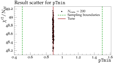
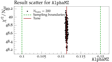
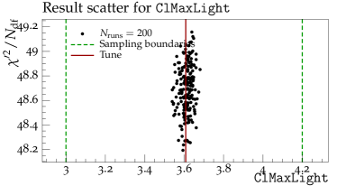
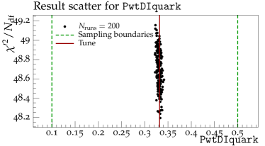
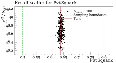
Fig. 1 shows the distributions for two hundred tunes based on two hundred randomly selected event samples points for the cubic interpolation. The spread of these values gives an idea of the systematics of the tuning process showing that we have obtained a good fit for our parameterisation of the generator response.
The line indicates the tune which is based on a cubic interpolation from six hundred event samples. It is this interpolation which was used to vary about the minimum to assess the uncertainty on the measured distributions. During the tune it was discovered that PSplitLight was relatively insensitive to the observables used in the tune. As such, PSplitLight was fixed at the default value of 1.20 during the tune and subsequent variation.
Professor was used to vary about the minimum value, as described above, determining the allowed range for the parameters. As five parameters were eventually varied, there are 10 new sample points - one for each of the parameters and one “+” and one “-” along each eigenvector direction in parameter space.
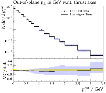
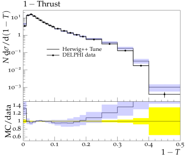
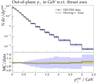
Various changes in were examined. A variation of keeps the LEP data within reasonable limits while a variation of is too large. The values for both and are shown in are shown in Tables 3 and Tables 3 respectively.
| Parameter | Direction | |||||||||
|---|---|---|---|---|---|---|---|---|---|---|
| 1 | 2 | 3 | 4 | 5 | ||||||
| + | - | + | - | + | - | + | - | + | - | |
| pTmin | 0.88 | 0.88 | 0.88 | 0.88 | 0.84 | 0.93 | 0.87 | 0.90 | 0.89 | 0.87 |
| AlphaMZ | 0.11 | 0.11 | 0.10 | 0.12 | 0.12 | 0.11 | 0.12 | 0.11 | 0.12 | 0.11 |
| ClMaxLight | 3.61 | 3.61 | 3.61 | 3.61 | 3.60 | 3.62 | 3.66 | 3.55 | 3.54 | 3.67 |
| PwtDIquark | 0.46 | 0.23 | 0.33 | 0.33 | 0.33 | 0.33 | 0.33 | 0.33 | 0.33 | 0.33 |
| PwtSquark | 0.64 | 0.64 | 0.64 | 0.64 | 0.64 | 0.64 | 0.62 | 0.67 | 0.51 | 0.78 |
| Parameter | Direction | |||||||||
|---|---|---|---|---|---|---|---|---|---|---|
| 1 | 2 | 3 | 4 | 5 | ||||||
| + | - | + | - | + | - | + | - | + | - | |
| pTmin | 0.88 | 0.88 | 0.88 | 0.88 | 0.82 | 0.95 | 0.86 | 0.90 | 0.89 | 0.87 |
| AlphaMZ | 0.11 | 0.11 | 0.10 | 0.12 | 0.12 | 0.10 | 0.12 | 0.10 | 0.12 | 0.11 |
| ClMaxLight | 3.61 | 3.61 | 3.61 | 3.61 | 3.59 | 3.63 | 3.68 | 3.52 | 3.52 | 3.70 |
| PwtDIquark | 0.51 | 0.19 | 0.33 | 0.33 | 0.33 | 0.33 | 0.33 | 0.33 | 0.33 | 0.33 |
| PwtSquark | 0.64 | 0.64 | 0.64 | 0.64 | 0.65 | 0.64 | 0.61 | 0.68 | 0.46 | 0.84 |
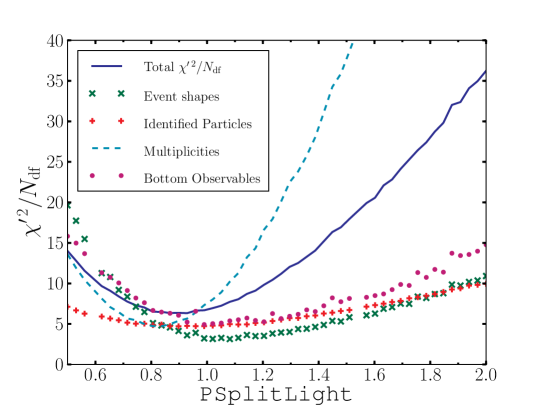
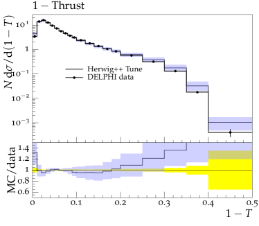
The Professor tune was then compared with the internal Herwig++ tuning procedure [29] as not all analyses that are in the internal Herwig++ tuning system are available in Rivet and subsequently accessible to Professor. Looking at Fig. 4 it is found that PSplitLight at a value of is favoured and gives a significant reduction in the . It was therefore decided to use the values obtained from minimisation procedure, but using the value of for PSplitLight to maintain a good overall description of the data. The new minima for the QCD parameters are summarized in the Table 1. Examples of the new tune and the uncertainty band are shown in Figs. 3 and 3 for the out-of-plane transverse momentum and thrust measured by DELPHI [45].
These error tune values can now be used to predict the uncertainty from the tuning of the shower parameters on any observable. In the next section we will present an example of using these tunes to estimate the uncertainty on the predictions for searches for the Higgs boson using the BDRS jet substructure method.
3 Jet Substructure Boosted Higgs
The analysis of Ref. [5] uses a number of different channels for the production of the Higgs boson decaying to in association with an electroweak gauge boson, i.e. the production of and . Ref. [5] uses the fact that the Higgs boson predominantly decays to in a jet substructure analysis to extract the signal of a boosted Higgs boson above the various backgrounds. Their study found that the Cambridge-Aachen algorithm [46, 47] with radius parameter gave the best results when combined with their jet substructure technique. For our study, we used the Cambridge-Aachen algorithm as implemented in the FastJet package [48]. Three different event selection criteria are used:
-
(a)
a lepton pair with and to select events for ;
-
(b)
missing transverse momentum to select events with ;
-
(c)
missing transverse momentum and a lepton with consistent with the presence of a boson with to select events with ;
where .
| Significance | |||
|---|---|---|---|
| Process | Order | ||
| Herwig++ default | Herwig++ tune | ||
| LO | 1.17 | ||
| NLO | 1.57 | ||
| LO | 2.18 | ||
| NLO | 2.95 | ||
| LO | 1.88 | ||
| NLO | 2.63 | ||
| Total | LO | 2.98 | |
| NLO | 4.09 | ||
In addition the presence of a hard jet with with substructure is required. The substructure analysis of Ref. [5] proceeds with the hard jet with some radius , a mass and in a mass-drop algorithm:
-
1.
the two subjets which were merged to form the jet, ordered such that the mass of the first jet is greater than that of the second jet , are obtained;
-
2.
if and
(2) where , and , , are the transverse momenta, rapidities and azimuthal angles of jets 1 and 2, respectively, then is in the heavy particle region. If the jet is not in the heavy particle region the procedure is repeated using the first jet.
This algorithm requires that are -tagged and takes and . A uniform -tagging efficiency of 60% was used with a uniform mistagging probability of 2%. The heavy jet selected by this procedure is considered to be the Higgs boson candidate jet. Finally, there is a filtering procedure on the Higgs boson candidate jet, . The jet, , is resolved on a finer scale by setting a new radius , where from the previous mass-drop condition, . The three hardest subjects of this filtering process are taken to be the Higgs boson decay products, where the two hardest are required to be -tagged.
All three analyses require that:
-
•
after the reconstruction of the vector boson, there are no additional leptons with pseudorapidity and ;
-
•
other than the Higgs boson candidate, there are no additional -tagged jets with pseudorapidity and .
In addition, due to top contamination, criterion (c) requires that other than the Higgs boson candidate, there are no additional -tagged jets with and . For all events, the candidate Higgs boson jet should have . The analyses were implemented using the Rivet system [44].
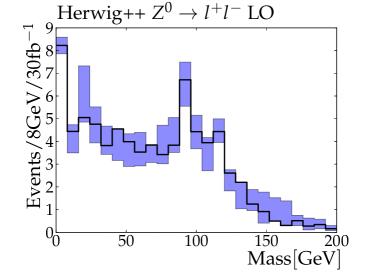
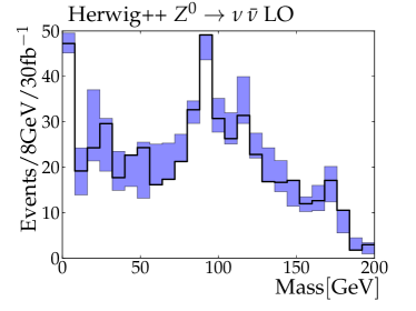
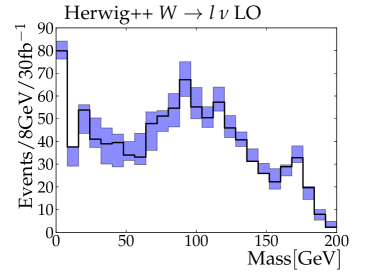
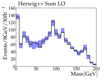
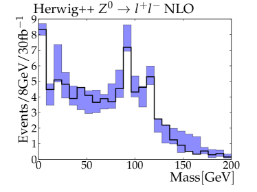
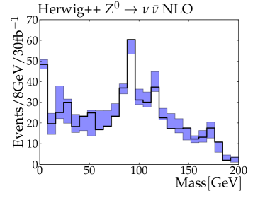
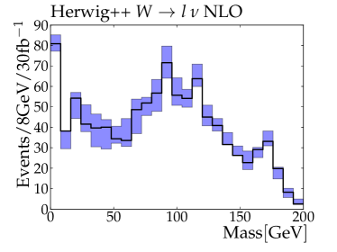
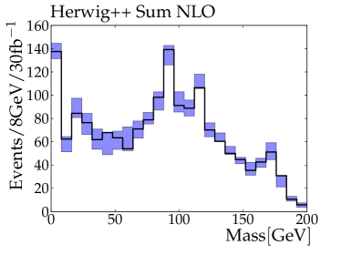
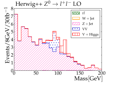
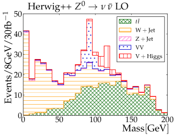
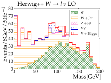
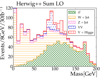
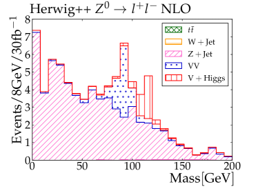
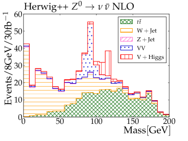
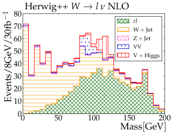
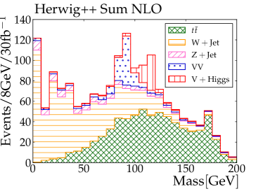
The plots shown in Fig. 5 use the leading-order matrix elements for the production and decay of Higgs boson but the , and top [49] have matrix element corrections for their decays. The plots shown in Fig. 6 have leading-order production, leading-order vector boson plus jet production (with the same matrix element corrections as the LO matrix elements) but the NLO vector boson pair production [50] and NLO vector and Higgs boson associated production [51]. In addition we have implemented the corrections to the decay in the POWHEG scheme, as described in Appendix B. The signal significances are outlined in Table 4.
The uncertainties due to the Monte Carlo simulation are shown as bands in Figs. 7 and 8. As there are correlations between the different processes the uncertainty is determined for the sum of all processes. Whilst it would be possible to show the envelope for the individual processes, this would not offer any information on the envelope for the sum of the processes which is the result of interest. In addition the uncertainty on the significance is shown in Table 4.
4 Conclusions
Monte Carlo simulations are an essential tool in the analysis of modern collider experiments. While significant effort has been devoted to the tuning of the parameters to produce a best fit there has been much less effort understanding the uncertainties in these results. In this paper we have produced a set of tunes which can be used to assess this uncertainty using the Herwig++ Monte Carlo event generator.
We then used these tunes to assess the uncertainties on the mass-drop analysis of Ref. [5] using Herwig++ with both leading- and next-to-leading-order matrix elements including a POWHEG simulation of the decay .
We find that while the jet substructure technique has significant potential as a Higgs boson discovery channel, we need to be confident of our tunes to investigate this with Monte Carlo simulations.
The error tunes and procedure here can now be used in other analyses where the uncertainty due to the Monte Carlo simulation is important.
5 Acknowledgements
We are grateful to all the other members of the Herwig++ collaboration and Hendrik Hoeth for valuable discussions and the authors of Ref. [5] for help in reproducing their results. We acknowledge the use of the UK Grid for Particle Physics in producing the results. This work was supported by the Science and Technology Facilities Council. DW acknowledges support by the STFC studentship ST/F007299/1.
Appendix A Observables and weights used to tune Herwig++
The weights and observables used in the Professor tuning system are outlined in the tables below.
| Observable | Weight | Observable | Weight |
|---|---|---|---|
| spectrum | 1.0 | spectrum | 1.0 |
| spectrum | 1.0 | spectrum | 1.0 |
| spectrum | 1.0 | spectrum | 1.0 |
| spectrum | 1.0 | spectrum | 1.0 |
| spectrum | 1.0 | spectrum | 1.0 |
| spectrum | 1.0 | spectrum | 1.0 |
| spectrum | 1.0 | spectrum | 1.0 |
| spectrum | 1.0 | spectrum | 1.0 |
| spectrum | 1.0 |
| Observable | Weight |
|---|---|
| Sphericity, | 1.0 |
| Energy-energy correlation, EEC | 1.0 |
| Aplanarity, | 2.0 |
| Mean out-of-plane in GeV w.r.t. thrust axes vs. | 1.0 |
| Mean charged multiplicity | 150.0 |
| Mean in GeV vs. | 1.0 |
| Planarity, | 1.0 |
| Thrust major, | 1.0 |
| Oblateness = | 1.0 |
| Out-of-plane in GeV w.r.t. sphericity axes | 1.0 |
| parameter | 1.0 |
| 1.0 | |
| Out-of-plane in GeV w.r.t. thrust axes | 1.0 |
| Log of scaled momentum, | 1.0 |
| In-plane in GeV w.r.t. sphericity axes | 1.0 |
| In-plane in GeV w.r.t. thrust axes | 1.0 |
| Thrust minor, | 2.0 |
| parameter | 1.0 |
| Scaled momentum, | 1.0 |
| Observable | Weight | Observable | Weight |
|---|---|---|---|
| Mean multiplicity | 10.0 | Mean multiplicity | 10.0 |
| Mean multiplicity | 10.0 | Mean multiplicity | 10.0 |
| Mean multiplicity | 10.0 | Mean multiplicity | 10.0 |
| Mean multiplicity | 10.0 | Mean multiplicity | 10.0 |
| Mean multiplicity | 10.0 | Mean multiplicity | 10.0 |
| Mean multiplicity | 10.0 | Mean multiplicity | 10.0 |
| Mean multiplicity | 10.0 | Mean multiplicity | 10.0 |
| Mean multiplicity | 10.0 | Mean multiplicity | 10.0 |
| Mean multiplicity | 10.0 | Mean multiplicity | 10.0 |
| Mean multiplicity | 10.0 | Mean multiplicity | 10.0 |
| Mean multiplicity | 10.0 | Mean multiplicity | 10.0 |
| Mean multiplicity | 10.0 | Mean multiplicity | 10.0 |
| Mean multiplicity | 10.0 | Mean multiplicity | 10.0 |
| Mean multiplicity | 10.0 | Mean multiplicity | 10.0 |
| Mean multiplicity | 10.0 | Mean multiplicity | 10.0 |
| Mean multiplicity | 10.0 | Mean multiplicity | 10.0 |
| Mean multiplicity | 10.0 | Mean multiplicity | 10.0 |
| Mean multiplicity | 10.0 | Mean multiplicity | 10.0 |
| Mean multiplicity | 10.0 | Mean multiplicity | 10.0 |
| Mean multiplicity | 10.0 | Mean multiplicity | 10.0 |
| Mean multiplicity | 10.0 | Mean multiplicity | 10.0 |
| Mean multiplicity | 10.0 | Mean multiplicity | 10.0 |
| Mean multiplicity | 10.0 | Mean multiplicity | 10.0 |
| Mean multiplicity | 10.0 | Mean multiplicity | 10.0 |
| Mean multiplicity | 10.0 | Mean multiplicity | 10.0 |
| Mean multiplicity | 10.0 |
| Observable | Weight |
|---|---|
| quark fragmentation function | 7.0 |
| Mean of quark fragmentation function | 3.0 |
Appendix B Simulation of using the POWHEG Method
The NLO differential decay rate in the POWHEG [39] approach is
| (3) |
where
| (4) |
Here is the leading-order Born differential decay rate, the regularized virtual contribution, the counter terms regularizing the real emission and the real emission contribution. The leading-order process has outgoing partons, with associated phase space . The virtual and Born contributions depend only on this -body phase space. The real emission phase space, , is factorised into the -body phase space and the phase space, , describing the radiation of an extra parton.
The Sudakov form factor in the POWHEG method is
| (5) |
where is the transverse momentum of the emitted parton.
In order to implement the decay of the Higgs boson in the POWHEG scheme in Herwig++ we need to generate the Born configuration according to Eq. 4 and the subsequent hardest emission according to Eq. 5. The generation of the truncated and vetoed parton showers from these configurations then proceeds as described in Refs.[29, 55, 51, 56].


The virtual contribution for was calculated in Ref. [57]. The corresponding real emission contribution, see Fig. 9, is
| (6) |
where is the leading-order matrix element, , is the mass of the bottom quark, is the mass of the Higgs boson, and . We use the Catani-Seymour subtraction scheme [58] where the counter terms are
| (7) |
where for , is the emitting parton and is the spectator parton. In practice, as the counter terms can become negative in some regions, we use
| (8) |
We have also regulated singularities in the virtual term with the integrated counter terms from the Catani-Seymour subtraction scheme allowing us to generate the Born configuration according to .
The hardest emission for each leg is generated according to
| (9) |
However this form is not suitable for the generation of the hardest emission. Instead we perform a Jacobian transformation and use the transverse momentum, , rapidity, , and azimuthal angle, , of the radiated gluon to define the phase space .
The momenta of the Higgs boson decay products are
| (10a) | ||||
| (10b) | ||||
| (10c) | ||||
where partons are the radiating bottom quark, spectator antibottom quark and radiated gluon, respectively. The energy fractions and. Using the conservation of momentum in the -direction and gives
| (11) |
Together with the definition, , we obtain the Jacobian
| (12) |
for the transformation of the radiation variables.
We can then generate the additional radiation according to Eq. B using the veto algorithm [3]. To achieve this we use an overestimate of the integrand in the Sudakov form factor, , where is a suitable constant. We first generate an emission according to
| (13) |
using this overestimate, where , , is the maximum possible transverse momentum of the gluon and is a parameter set in the model, taken to be .
The trial value of the transverse momentum is obtained by solving , where is a random number in , i.e.
| (14) |
Once the trial has been generated, and are also generated uniformly between and , respectively. The energy fractions of the partons are obtained using the definition ,
| (15) |
and using energy conservation. As there are two solutions for both solutions must be kept and used to calculate the weight for a particular trial . The signs of the -components of the momenta are fixed by the sign of the rapidity and momentum conservation. Any momentum configurations outside of the physically allowed phase space are rejected and a new set of variables generated. The momentum configuration is accepted with a probability given by the ratio of the true integrand to the overestimated value. If the configuration is rejected, the procedure continues with set to the rejected until the trial value of is accepted or falls below the minimum allowed value, . This procedure generates the radiation variables correctly as shown in Ref. [3].
This procedure is used to generate a trial emission from both the bottom and antibottom. The hardest potential emission is then selected which correctly generates events according to Eq. B using this competition algorithm.
References
- [1] P. Z. Skands, Tuning Monte Carlo Generators: The Perugia Tunes, Phys.Rev. D82 (2010) 074018, [arXiv:1005.3457].
- [2] B. Cooper, J. Katzy, M. Mangano, A. Messina, L. Mijovic, et. al., Monte Carlo tuning in the presence of Matching, arXiv:1109.5295.
- [3] T. Sjöstrand, S. Mrenna, and P. Skands, PYTHIA 6.4 Physics and Manual, JHEP 05 (2006) 026, [hep-ph/0603175].
- [4] A. Buckley, H. Hoeth, H. Lacker, H. Schulz, and J. E. von Seggern, Systematic event generator tuning for the LHC, Eur. Phys. J. C65 (2010) 331–357, [arXiv:0907.2973].
- [5] J. M. Butterworth, A. R. Davison, M. Rubin, and G. P. Salam, Jet substructure as a new Higgs search channel at the LHC, Phys. Rev. Lett. 100 (2008) 242001, [arXiv:0802.2470].
- [6] S. D. Ellis, C. K. Vermilion, and J. R. Walsh, Techniques for improved heavy particle searches with jet substructure, Phys. Rev. D80 (2009) 051501, [arXiv:0903.5081].
- [7] S. D. Ellis, C. K. Vermilion, and J. R. Walsh, Recombination Algorithms and Jet Substructure: Pruning as a Tool for Heavy Particle Searches, Phys. Rev. D81 (2010) 094023, [arXiv:0912.0033].
- [8] G. D. Kribs, A. Martin, T. S. Roy, and M. Spannowsky, Discovering the Higgs Boson in New Physics Events using Jet Substructure, Phys. Rev. D81 (2010) 111501, [arXiv:0912.4731].
- [9] G. D. Kribs, A. Martin, T. S. Roy, and M. Spannowsky, Discovering Higgs Bosons of the MSSM using Jet Substructure, Phys. Rev. D82 (2010) 095012, [arXiv:1006.1656].
- [10] G. D. Kribs, A. Martin, and T. S. Roy, Higgs Discovery through Top-Partners using Jet Substructure, arXiv:1012.2866.
- [11] J. M. Butterworth, J. R. Ellis, A. R. Raklev, and G. P. Salam, Discovering baryon-number violating neutralino decays at the LHC, Phys.Rev.Lett. 103 (2009) 241803, [arXiv:0906.0728].
- [12] CDF Collaboration Collaboration, T. Aaltonen et. al., Study of Substructure of High Transverse Momentum Jets Produced in Proton-Antiproton Collisions at TeV, arXiv:1106.5952.
- [13] Y. Bai and J. Shelton, Composite Octet Searches with Jet Substructure, arXiv:1107.3563.
- [14] C. K. Vermilion, Jet Substructure at the Large Hadron Collider: Harder, Better, Faster, Stronger, arXiv:1101.1335. Ph.D.Thesis.
- [15] T. Plehn, G. P. Salam, and M. Spannowsky, Fat Jets for a Light Higgs, Phys.Rev.Lett. 104 (2010) 111801, [arXiv:0910.5472].
- [16] M. H. Seymour, Searches for new particles using cone and cluster jet algorithms: A Comparative study, Z.Phys. C62 (1994) 127–138.
- [17] A. Abdesselam, E. B. Kuutmann, U. Bitenc, G. Brooijmans, J. Butterworth, et. al., Boosted objects: A Probe of beyond the Standard Model physics, Eur.Phys.J. C71 (2011) 1661, [arXiv:1012.5412].
- [18] I. Feige, M. Schwartz, I. Stewart, and J. Thaler, Precision Jet Substructure from Boosted Event Shapes, arXiv:1204.3898.
- [19] A. Altheimer, S. Arora, L. Asquith, G. Brooijmans, J. Butterworth, et. al., Jet Substructure at the Tevatron and LHC: New results, new tools, new benchmarks, J.Phys.G G39 (2012) 063001, [arXiv:1201.0008].
- [20] S. Yang and Q.-S. Yan, Searching for Heavy Charged Higgs Boson with Jet Substructure at the LHC, JHEP 1202 (2012) 074, [arXiv:1111.4530].
- [21] J. M. Butterworth, B. E. Cox, and J. R. Forshaw, WW scattering at the CERN LHC, Phys. Rev. D65 (2002) 096014, [hep-ph/0201098].
- [22] J. M. Butterworth, J. R. Ellis, and A. R. Raklev, Reconstructing sparticle mass spectra using hadronic decays, JHEP 05 (2007) 033, [hep-ph/0702150].
- [23] Measurement of jet mass and substructure for inclusive jets in √s = 7 tev pp collisions with the atlas experiment, Tech. Rep. ATLAS-CONF-2011-073, CERN, Geneva, May, 2011.
- [24] Atlas sensitivity to the standard model higgs in the hw and hz channels at high transverse momenta, Tech. Rep. ATL-PHYS-PUB-2009-088, CERN, Geneva, Aug, 2009.
- [25] Study of jet substructure in pp collisions at 7 tev in cms, Tech. Rep. CMS PAS JME 10-013, CERN, Geneva, March, 2011.
- [26] G. Corcella et. al., HERWIG 6: An event generator for Hadron Emission Reactions with Interfering Gluons (including supersymmetric processes), JHEP 01 (2001) 010, [hep-ph/0011363].
- [27] G. Corcella et. al., HERWIG 6.5 Release Note, hep-ph/0210213.
- [28] J. M. Butterworth, J. R. Forshaw, and M. H. Seymour, Multi-Parton Interactions in Photoproduction at HERA, Z. Phys. C72 (1996) 637–646, [hep-ph/9601371].
- [29] M. Bähr et. al., Herwig++ Physics and Manual, Eur. Phys. J. C58 (2008) 639–707, [arXiv:0803.0883].
- [30] K. Arnold, L. d’Errico, S. Gieseke, D. Grellscheid, K. Hamilton, et. al., Herwig++ 2.6 Release Note, arXiv:1205.4902.
- [31] G. Marchesini and B. R. Webber, Simulation of QCD Coherence in Heavy Quark Production and Decay, Nucl. Phys. B330 (1990) 261.
- [32] S. Gieseke, P. Stephens, and B. Webber, New Formalism for QCD Parton Showers, JHEP 12 (2003) 045, [hep-ph/0310083].
- [33] M. Bähr, S. Gieseke, and M. H. Seymour, Simulation of multiple partonic interactions in Herwig++, 0803.3633.
- [34] M. Bähr, J. M. Butterworth, and M. H. Seymour, The Underlying Event and the Total Cross Section from Tevatron to the LHC, arXiv:0806.2949.
- [35] S. Gieseke, C. Röhr, and A. Siodmok, Colour reconnections in Herwig++, arXiv:1206.0041.
- [36] S. Gieseke, C. Röhr, and A. Siodmok, Multiple Partonic Interaction Developments in Herwig++, arXiv:1110.2675.
- [37] ATLAS Collaboration Collaboration, G. Aad et. al., Jet mass and substructure of inclusive jets in sqrt(s) = 7 TeV pp collisions with the ATLAS experiment, JHEP 1205 (2012) 128, [arXiv:1203.4606].
- [38] ATLAS Collaboration Collaboration, G. Aad et. al., ATLAS measurements of the properties of jets for boosted particle searches, arXiv:1206.5369.
- [39] P. Nason, A new method for combining NLO QCD with shower Monte Carlo algorithms, JHEP 11 (2004) 040, [hep-ph/0409146].
- [40] S. Frixione, P. Nason, and C. Oleari, Matching NLO QCD computations with Parton Shower simulations: the POWHEG method, JHEP 11 (2007) 070, [0709.2092].
- [41] B. R. Webber, A QCD Model for Jet Fragmentation including Soft Gluon Interference, Nucl. Phys. B238 (1984) 492.
- [42] D. Amati and G. Veneziano, Preconfinement as a Property of Perturbative QCD, Phys. Lett. B83 (1979) 87.
- [43] A. Buckley et. al., General-purpose event generators for LHC physics, arXiv:1101.2599.
- [44] A. Buckley, J. Butterworth, L. Lönnblad, H. Hoeth, J. Monk, et. al., Rivet user manual, arXiv:1003.0694.
- [45] DELPHI Collaboration, P. Abreu et. al., Tuning and Test of Fragmentation Models based on Identified Particles and Precision Event Shape Data, Z. Phys. C73 (1996) 11–60.
- [46] Y. L. Dokshitzer, G. D. Leder, S. Moretti, and B. R. Webber, Better Jet Clustering Algorithms, JHEP 08 (1997) 001, [hep-ph/9707323].
- [47] M. Wobisch, Measurement and QCD analysis of jet cross sections in deep-inelastic positron proton collisions at s**(1/2) = 300-GeV, . DESY-THESIS-2000-049.
- [48] M. Cacciari and G. P. Salam, Dispelling the myth for the jet-finder, Phys. Lett. B641 (2006) 57–61, [hep-ph/0512210].
- [49] K. Hamilton and P. Richardson, A Simulation of QCD Radiation in Top Quark Decays, JHEP 02 (2007) 069, [hep-ph/0612236].
- [50] K. Hamilton, A positive-weight next-to-leading order simulation of weak boson pair production, JHEP 1101 (2011) 009, [arXiv:1009.5391].
- [51] K. Hamilton, P. Richardson, and J. Tully, A Positive-Weight Next-to-Leading Order Monte Carlo Simulation for Higgs Boson Production, JHEP 04 (2009) 116, [arXiv:0903.4345].
- [52] ALEPH Collaboration, R. Barate et. al., Studies of Quantum Chromodynamics with the ALEPH detector, Phys. Rept. 294 (1998) 1–165.
- [53] Particle Data Group Collaboration, C. Amsler et. al., Review of Particle Physics, Phys.Lett. B667 (2008) 1–1340.
- [54] G. Barker, E. Ben-Haim, M. Feindt, U. Kerzel, P. Roudeau, L. Ramler, and A. Savoy-Navarro, A study of the b-quark fragmentation function with the delphi detector at lep i. oai:cds.cern.ch:994376, Tech. Rep. DELPHI-2002-069-CONF-603. CERN-DELPHI-2002-069-CONF-603, CERN, Geneva, Jul, 2002.
- [55] K. Hamilton, P. Richardson, and J. Tully, A Positive-Weight Next-to-Leading Order Monte Carlo Simulation of Drell-Yan Vector Boson Production, arXiv:0806.0290.
- [56] L. D’Errico and P. Richardson, A Positive-Weight Next-to-Leading-Order Monte Carlo Simulation of Deep Inelastic Scattering and Higgs Boson Production via Vector Boson Fusion in Herwig++, arXiv:1106.2983.
- [57] E. Braaten and J. P. Leveille, Higgs Boson Decay and the Running Mass, Phys. Rev. D22 (1980) 715.
- [58] S. Catani, S. Dittmaier, M. H. Seymour, and Z. Trócsányi, The Dipole Formalism for Next-to-Leading Order QCD Calculations with Massive Partons, Nucl. Phys. B627 (2002) 189–265, [hep-ph/0201036].