The properties of the local spiral arms from RAVE data: two-dimensional density wave approach

Abstract

Using the RAVE survey, we recently brought to light a gradient in the mean galactocentric radial velocity of stars in the extended solar neighbourhood. This gradient likely originates from non-axisymmetric perturbations of the potential, among which a perturbation by spiral arms is a possible explanation. Here, we apply the traditional density wave theory and analytically model the radial component of the two-dimensional velocity field. Provided that the radial velocity gradient is caused by relatively long-lived spiral arms that can affect stars substantially above the plane, this analytic model provides new independent estimates for the parameters of the Milky Way spiral structure. Our analysis favours a two-armed perturbation with the Sun close to the inner ultra-harmonic 4:1 resonance, with a pattern speed $\Omega_{p}=18.6^{+0.3}_{-0.2}\,\mathrm{km\,s}^{-1}\,\mathrm{kpc}^{-1}\,$ and a small amplitude $A=0.55^{+0.02}_{-0.02}\%$ of the background potential (14% of the background density). This model can serve as a basis for numerical simulations in three dimensions, additionally including a possible influence of the galactic bar and/or other non-axisymmetric modes.

1 Introduction

It has long been recognized that internal secular evolution processes should play a major role in shaping galaxy disks. Among the main drivers of this secular evolution are the disc instabilities and associated non-axisymmetric perturbations, including the bar and spiral arms. Questions about their nature – transient or quasi-stationary (e.g., Sellwood 2010a; Quillen et al. 2011; Grand et al. 2012a) – , about their detailed structure and dynamics such as their amplitude, pattern speed, pitch angle or number of arms, as well as questions about their detailed influence on secular processes like stellar migration (Sellwood & Binney 2002; Minchev & Famaey 2010), are all essential elements for a better understanding of galactic evolution. The Milky Way provides a unique laboratory in which a snapshot of the dynamical effect of present-day disc non-axisymmetries can be studied in great detail, and help answering the above questions.

Current knowledge of the structure and dynamics of the bar and the spiral arms of the Milky Way relies both on the gas, and notably on its observed longitude-velocity diagram (Binney et al. 1991; Bissantz et al. 2003; Englmaier et al. 2011) or masers in high mass star forming regions (Reid et al. 2009, and references therein), and on the stars (e.g., Georgelin & Georgelin 1976; Binney, Gerhard & Spergel 1997; Stanek et al. 1997; Benjamin et al. 2005; Lépine et al. 2011b). For the spiral arms, both types of constraints are combined in a recent study by Vallée (2008), whose model predicts the location in space and velocity for the spiral arms.

With the advent of new spectroscopic and astrometric surveys, six-dimensional phase-space information for stars in an increasingly large volume around the Sun allow us to set new dynamical constraints on the non-axisymmetric perturbations of the Galactic potential. An example of such new detailed kinematical information on stellar motions in the extended solar neighbourhood is the recently detected (galactocentric) radial velocity gradient of $\sim 4\,\mathrm{km\,s}^{-1}\,\mathrm{kpc}^{-1}\,$ by Siebert et al. (2011a), making use of more than 200 thousand stars from the RAVE survey. If this result is not owing to systematic distance errors (which the geometry of the radial velocity flow seems to exclude by not depending on distance and longitude in any systematically biased way), and more importantly, if one assumes that, at first order, what is seen above the plane is a reflection of what would happen in a razor-thin disc, and that the spiral arms are long-lived, one can apply the analytic density wave description of spiral arms proposed by Lin & Shu (1964) to constrain the shape, amplitude and dynamics of spiral arms.

Whether long-lived density waves are the correct description of spiral patterns in galaxies remains heavily debated. From a theoretical point of view, while it seems that the radial velocity dispersion profile needed to support long-lived spiral waves in barless discs (e.g., Bertin & Lin 1996) would be heavily unstable (Sellwood 2010a), the situation is much less clear in the presence of a central bar, where nonlinear mode coupling between the bar and spiral could sustain a long-lived spiral pattern (Voglis et al. 2006; Salo et al. 2010; Quillen et al. 2011; Minchev et al. 2012), while Grand et al. (2012b) however find that spiral arms are transient even in the presence of a central bar. On the other hand, D’Onghia et al. (2012) find locally long-lived self-perpetuating spiral arms which could be locally consistent with density waves, but fluctuating in amplitude with time. Furthermore, long-lived spirals can also develop as being sustained by coherent oscillations due to a flyby galaxy encounter (Struck et al. 2011), a process we know to be ongoing for the Milky Way, and cosmologically simulated disk galaxies exhibit a distribution of young stars consistent with the predictions of classical density wave theory for long-lived spirals (Pilkington et al. 2012). Finally, let us note that both long-lived and transient spirals can coexist in a galaxy, which adds complexity to the picture.

On the observational side the situation is also unclear. Evidence seems to exist for both transient and long-lived spiral arms: e.g., M81 apparently contains long-lived spiral arms consistent with the classical density wave theory (Lowe et al. 1994; Adler & Wefstpfahl 1996; Kendall et al. 2008) while in M51, even if its disc streaming motion appears consistent with the density wave description, the mass fluxes are inconsistent with a steady flow (Shetty 2007). Studying observational tracers for different stages of the star-formation sequence in 12 nearby spiral galaxies, Foyle et al. (2011) also found that they do not show the expected spatial ordering for long-lived spiral arms, from upstream to downstream in the corotating frame. In the Milky Way, many of the dynamical constraints on spiral arms currently come from local constraints provided by velocity space substructures also known as moving groups (Dehnen 1998; Famaey et al. 2005). For instance, examining the local stellar distribution in action space, Sellwood (2010b) found that stars from the Hyades moving group were concentrated along a resonance line in action space, which was interpreted as a signature of scattering at the inner Lindblad resonance of a transient spiral pattern (see also McMillan 2011, who found that this feature could also be associated with an outer Lindblad resonance). However, in this picture, only the Hyades moving group is accounted for, and the remaining substructures observed in the local phase space distribution must be explained by invoking other origins. Models based only on transient spiral arms (e.g., De Simone et al. 2004) were actually unable to reproduce the precise location of the various other prominent moving groups, such as Sirius. On the other hand, models based on long-lived spiral arms, locating the 4:1 inner resonance close to the Sun, were able to reproduce both the position of the Hyades and Sirius moving groups at the same time (Quillen & Minchev 2005; Pompéia et al. 2011) as well as other moving groups (Antoja et al. 2011). Other observational arguments based on the step-like metallicity gradient in the Galactic disc also argue in favor of long-lived spirals (Lépine et al. 2011).

Given this theoretical and observational situation, we here make the conservative assumption that interesting information can be retrieved from the classical analytic treatment of spiral arms as long-lived density waves. This analytic model could then serve as a basis for numerical simulations in a three-dimensional disc. The paper is structured as follows. In Section 2, we review the data, as well as the analytic density wave model we are using. We present and discuss our results in Section 3, and conclude in Section 4.

2 Data & Method

2.1 Two-dimensional velocity field

Our analysis is based on data from the RAVE survey (Steinmetz et al. 2006; Zwitter et al. 2008; Siebert et al. 2011b) which provides line-of-sight velocities with a precision of 2 $\mathrm{km\,s}^{-1}$for a large number of bright stars in the southern hemisphere with $9<I<12$. RAVE selects its targets randomly in the I-band interval, and so its properties are similar to a magnitude limited survey. The RAVE catalogue is cross-matched with astrometric (PPMX, UCAC2, Tycho-2) and photometric catalogues (2MASS, DENIS) to provide additional proper motions and magnitudes. In this study, we use the internal version of the catalogue which contains data for 434,807 spectra (393,903 stars). To compute the galactocentric velocities, knowledge of the distance to the star is required. For RAVE stars, distances to 30% are available in three studies: Breddels et al. (2010), Zwitter et al. (2010) and Burnett et al. (2011). All catalogues provide compatible distance estimators and the velocity maps generated using the different catalogues are similar.

Our final sample consists of 213,713 stars from this survey limited to a distance of 2 kpc from the Sun and to a height of 1 kpc above and below the plane. We demonstrated the existence of a velocity gradient of disc stars in the fourth quadrant, directed radially from the Galactic centre (Siebert et al. 2011a). The two-dimensional mean galactocentric radial velocity field in the Galactic plane is presented in Fig. 1 where we use a box $4\times 4$ kpc in size, centered on the Sun, sampled using 60 bins in each directions. For this analysis, we restrict ourselves to bins containing more than 5 stars and the mean velocity is computed using a median function. Note that converting velocities in the heliocentric reference frame into the $(V_{R},V_{\theta})$ galactocentric coordinates requires the galactocentric radius of the Sun $R_{0}$, the Sun’s peculiar velocity $\textbf{v}_{\odot}$ with respect to the Local Standard of Rest (LSR), and the motion of the LSR with respect to the Galactic center $\textbf{v}_{\mathrm{LSR}}$. We assume $R_{0}=8\,$kpc for the distance of the Sun to the Galactic centre and $V_{\mathrm{LSR}}=220\,\mathrm{km\,s}^{-1}\,$ to match the values used for the mass model (see Section 2.2). We use the latest determination of the value of the solar motion by Schönrich et al. (2010): $(U_{\odot},V_{\odot})=(11.1,12.24)\,\mathrm{km\,s}^{-1}\,$.

The gradient affects a sample dominated at large distances by red giants, with a typical velocity dispersion $\sigma_{R}\sim$ 30–40$\mathrm{km\,s}^{-1}$, and affects stars substantially above the plane, keeping in mind that RAVE lines of sight are typically at $|b|>\sim 20^{\circ}$. The zone where the gradient is the steepest is populated with stars with typically $|z|\sim 500\,$pc. However, if $U_{\mathrm{LSR}}$ is positive (a local mean motion towards the inner Galaxy), then $\,\langle V_{R}\rangle\,$would be by construction negative in the Sun’s neighbourhood and reach $0$ at larger distances and larger heights. In the modelling procedure hereafter, we let $\,\langle V_{R}\rangle_{R_{0}}\,\equiv-U_{\mathrm{LSR}}$ be a parameter of the model to allow us to account for uncertainties on this quantity.

Ideally one would also use the tangential velocity field $\langle V_{\theta}\rangle$ in combination to the $\,\langle V_{R}\rangle\,$field. However, as stated above, our sample reaches distances to the Galactic plane of 1 kpc, avoiding the regions close to the plane. The RAVE survey mimicking a magnitude limited survey in fields 6$\,\deg$ in diameter on the sky, each field containing a different number of stars, the stellar population mixture varies from point to point on the maps. Therefore, the contribution of the asymmetric drift is difficult to estimate while it enters the calculation of the $V_{\theta}$ component. Hence, we chose to restrict our analysis to the $\,\langle V_{R}\rangle\,$field, although we give the full set of equations, including this component, in the next section.

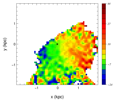
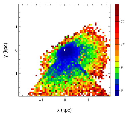
Figure 1: Left: velocity field for the radial component of the velocity vector $\,\langle V_{R}\rangle\,$as a function of location in the Galactic plane. Right: associated random error on the mean velocity. In both panels, the location of the Sun is marked by a star, the Galactic centre is towards positive x and the y-axis is oriented towards the Galactic rotation. The colour coding follows the mean velocity and mean velocity error in $\mathrm{km\,s}^{-1}$.

2.2 Density Wave model

To model the velocity field, we use the density wave description of spiral arms proposed by Lin & Shu (1964) and further developed in Lin, Yuan & Shu (1969) and Shu, Stachnik & Yost (1971). This model is based on an asymptotic analysis of the WKBJ type of the Euler/Boltzmann equations, valid only in the regime of weak, long-lived and tightly wound spirals (small pitch angle). This model being well known and documented (see for example Binney & Tremaine 2008), we restrict its description to the main results used in this study.

The perturbation to the potential considered is of the form

$$\Phi_{1}=A(R)\exp\big{[}i(\omega t-m\theta+\Phi(R))\big{]}\,,$$ (1)

where $A(R)$ is the amplitude of the perturbation, $m$ is the number of arms and $\Phi(R)$ is a monotonic function. The perturbation rotates at an angular frequency given by

$$\Omega_{\mathrm{p}}=\omega/m\,.$$ (2)

The perturbations in the components of the mean velocities $\,\langle V_{R}\rangle\,$and $\langle V_{\theta}\rangle$, where $(R,\theta)$ are the coordinates in the cylindrical coordinate system centered on the Galaxy, are given by

$$\langle V_{R}\rangle = \frac{kA}{\kappa}\frac{\nu}{1-\nu^{2}}{\cal F}_{\nu}^{(1)}(x)\cos(\chi)$$

$$\langle V_{\theta}\rangle = -\frac{1}{2}\frac{kA}{\Omega}\frac{1}{1-\nu^{2}}{\cal F}_{\nu}^{(2)}(x)\sin(\chi)$$ (3)

where

$$x=\frac{k^{2}\sigma^{2}_{R}}{\kappa^{2}}\,,$$ (4)

$k$ being the radial wave number, $\sigma_{R}$ the velocity dispersion, $\kappa$ the epicyclic frequency and $\nu$ is defined by $\nu=m(\Omega_{\mathrm{p}}-\Omega)/\kappa$.

The functions ${\cal F}_{\nu}^{(1)}$ and ${\cal F}_{\nu}^{(2)}$ are the “reduction factors” that correct the mean velocities for the effect of velocity dispersion, lowering the effect of the spiral perturbation on the velocity field as the velocity dispersion increases. In the limit of a zero velocity dispersion (${\cal F}_{\nu}^{(1)}={\cal F}_{\nu}^{(2)}=1$) we recover the velocity field of the gas while if $\sigma_{R}$ becomes large, ${\cal F}_{\nu}^{(1)}={\cal F}_{\nu}^{(2)}\rightarrow 0$ and the velocity field becomes unaffected by the spiral perturbation. The two functions are given in Appendix B of Lin, Yuan & Shu (1969).

The phase of the spiral pattern $\chi$ is defined by

$$\chi=\omega t-m\theta+\Phi(R)$$ (5)

which, in the case of logarithmic spirals with $\Phi(R)=m\,\mathrm{cotg}\,i\,\ln R$ in Eq. 1 ($i$ being the pitch angle), can be written in a more convenient form

$$\chi=\chi_{0}+m(\mathrm{cotg}\,i\,\ln(R/R_{0})-(\theta-\theta_{0}))\,.$$ (6)

The subscripts $0$ in the previous equation refer to the value at the Sun’s location. The radial wave number $k$ is then given by

$$k(R)=\Phi^{\prime}(R)=m\,\mathrm{cotg\,}i/R\,,$$ (7)

with $k(R)<0$ for trailing waves and $k(R)>0$ for leading waves.

The mean velocities of Eq. 3 vary in the Galactic plane as a function of $R$ and $\theta$, the modulation depending on the mass model via $\Omega$ and $\kappa$, the velocity dispersion in the radial direction $\sigma_{R}$ via the reduction factors and on the parameters of the spiral perturbation. These parameters are the number of arms $m$, the amplitude of the perturbation $A$, its pattern speed $\Omega_{\mathrm{p}}$, the pitch angle $i$ and the phase $\chi_{0}$. In addition we chose to include $\,\langle V_{R}\rangle_{R_{0}}\,$ as a free parameter while computing the model to account for possible uncertainties on $U_{\mathrm{LSR}}$. While this parameter is usually taken into account while computing the velocities ($V_{R},V_{\theta}$) of the observations, here we include it as a correction to the predicted $\,\langle V_{R}\rangle\,$and $\langle V_{\theta}\rangle\,$ in the model to avoid the computation of the velocity field at each step which is time consumming. In the remainder of the paper, we will denote $\mathbf{P}$ the vector of model parameters $\mathbf{P}=(m,A,\Omega_{\mathrm{p}},i,\chi_{0},\sigma_{R},\,\langle V_{R}\rangle_{R_{0}}\,)$.

For the rotation curve of the Milky Way, we use the models I and II of Binney & Tremaine (2008) Table 2.3, based on the mass models of Dehnen & Binney (1998). These models reproduce equally well the circular-speed curve and other observationally constrained quantities such as the Oort constants, the surface mass density within 1.1 kpc or the total mass within 100 kpc of the Milky Way. The two models correspond to two limiting cases where either the disc or the halo dominates the rotation curve (model I and II respectively). The models being computed for $R_{0}=8$ kpc and $V_{co}\sim 220$ $\mathrm{km\,s}^{-1}$, we use the same values for these two parameters when computing the galactocentric velocities in Fig. 1.

In practice, our tests showed that all our solutions converged on approximately the same value for $\sigma_{R}$. This is due to our sample being dominated by the old thin disc population and we chose to fix $\sigma_{R}$ to the best fit value, $\sigma_{R}=34.2\,\mathrm{km\,s}^{-1}\,$, to reduce the dimension of our parameter space. This value of the dispersion fits very well the observed dispersion from the RAVE sample, excluding the tails representative of the thick disc population and of large proper motion errors. Hence, the model parameters we consider in the remainder of the paper is $\mathbf{P}=(m,A,\Omega_{\mathrm{p}},i,\chi_{0},\,\langle V_{R}\rangle_{R_{0}}\,)$.

The mean velocities of Eq. 3 are compared to the two dimensional velocity field of Section 2.1. The comparison is done using a chi–square estimator

$$\chi^{2}=\sum_{i}\frac{(\,\langle V_{R}\rangle_{i,obs}\,-\langle V_{R}\rangle_{i,model}\,)^{2}}{\sigma^{2}_{i,obs}}\,,$$ (8)

where the sum is on all bins containing at least 5 stars and $\sigma_{i,obs}$ is the error on the mean velocity shown in Fig. 1 right panel. We restrict the analysis to the mean velocity in the radial direction, the tangential velocities being affected by the asymmetric drift which can not be properly taken into account in the model, our sample being a mixture of stellar populations of different ages, even though it is dominated by the old thin disc (see Section 2.1).

We note also that systematic distance errors would affect the results presented below. As shown in the first paper (Siebert et al. 2011a), a systematic error in the distances affects the measured gradient in $\,\langle V_{R}\rangle\,$by approximately the same factor: a 20% overestimate/underestimate of the distances induces a $\sim 20$% overestimate/understimate of the amplitude of the velocity gradient in $\,\langle V_{R}\rangle\,$, which to first order, results in a higher/lower amplitude $A$ of the spiral perturbation by the same amount. However, as shown in the same paper, an independent estimate of the velocity field using red clump stars, for which an unbiased distance estimate can be obtained, shows a good agreement of the velocity fields, giving us confidence that our distances can not be strongly affected by an unknown bias and we will not consider this possibility in the remainder in this paper.

3 Results and discussion

3.1 Parameter space sampling

The number of arms in the Milky Way is not known with certainty. Both 2-armed and 4-armed spiral pattern are considered in the literature although an $m=2$ mode in the stars seems to be favoured. In the analysis we will consider both cases and look for the best matching solution for either number of spiral arms.

Also, some recent works have suggested that the local standard of rest is not on a circular orbit, eg. $U_{\mathrm{LSR}}$ might not be 0 $\mathrm{km\,s}^{-1}$(Smith et al. 2009; Smith, Whiteoak & Evans 2012; Moni-Bidin, Carraro & Mendez 2012). Therefore, we include the possibility for a non-null $U$ component of the LSR in the model.

For the minimisation, we considered the standard value of $U_{\mathrm{LSR}}=0\,\mathrm{km\,s}^{-1}\,$ as well as values of $\pm 5$ $\mathrm{km\,s}^{-1}$whose amplitude correspond to the finding of Smith, Whiteoak & Evans (2012). Finally we left $\,\langle V_{R}\rangle_{R_{0}}\,$ as a free parameter in the fit. However, we note that our sample reaches only 2 kpc away from the Sun, not deep enough in the plane to disentangle the effect of a radial motion of the LSR from uncertainties in the $U$ component of the solar motion with respect to the LSR. Therefore we should keep in mind that a non-null best fit value of the $\,\langle V_{R}\rangle_{R_{0}}\,$ parameter does not necessarily imply a radial motion of the LSR.

The summary of the chi-square analysis is presented in Table 1 and the chi-square contours for the best models are presented in Fig. 2. In this figure, the two panels show the 1, 2 and 3-$\sigma$ contours, fixing all the other parameters to the best fit solution, in the $\Omega_{p}$ versus amplitude plane (left panel) and pitch angle $i$ versus phase $\chi_{0}$ (right panel). The plain lines are for the mass model I, the red dashed lines for model II.

Table 1: Chi-square results. Parameters with error bars were kept free in the minimisation. The error bars correspond to the 1-$\sigma$ internal errors obtained from the chi-square contour. Models marked with (*) have a large pitch angle (open arms) and do not satisfy the tight-winding approximation. The number of pixels used in the minimisation procedure is 1595.

Mass	$m$	$\,\langle V_{R}\rangle_{R_{0}}\,$	$\Omega_{p}$	$A$	$i$	$\chi_{0}$	$\chi^{2}$
model		$\mathrm{km\,s}^{-1}$	$\,\mathrm{km\,s}^{-1}\,\mathrm{kpc}^{-1}\,$	% (total, disc)	deg	deg
I	2	$0.9^{+0.1}_{-0.1}$	$18.9^{+0.3}_{-0.2}$	$(0.50^{+0.02}_{-0.02},2.27^{+0.08}_{-0.07})$	$-10.0^{+0.4}_{-0.4}$	$76.9^{+1.1}_{-1.2}$	1829.00
I	2	-5	$16.1^{+0.1}_{-0.1}$	$(0.78^{+0.01}_{-0.01},3.50^{+0.07}_{-0.06})$	$-23.2^{+0.3}_{-0.5}$	$57.3^{+0.6}_{-0.5}$	1943.14	(*)
I	2	0	$18.8^{+0.2}_{-0.3}$	$(0.49^{+0.02}_{-0.02},2.21^{+0.08}_{-0.09})$	$-9.1^{+0.3}_{-0.4}$	$65.8^{+1.5}_{-1.0}$	1831.99
I	2	5	$19.3^{+0.1}_{-0.2}$	$(0.69^{+0.02}_{-0.01},3.12^{+0.09}_{-0.05})$	$-15.6^{+0.7}_{-0.6}$	$112.1^{+1.0}_{-0.9}$	1853.04
II	2	$0.9^{+0.3}_{-0.2}$	$18.6^{+0.3}_{-0.2}$	$(0.55^{+0.02}_{-0.02},3.09^{+0.10}_{-0.13})$	$-10.0^{+0.4}_{-0.4}$	$76.0^{+1.3}_{-1.0}$	1828.46
II	2	-5	$15.1^{+0.1}_{-0.1}$	$(0.71^{+0.01}_{-0.01},3.93^{+0.06}_{-0.07})$	$-22.3^{+0.3}_{-0.6}$	$55.7^{+0.7}_{-0.4}$	1940.75	(*)
II	2	0	$18.5^{+0.3}_{-0.2}$	$(0.54^{+0.02}_{-0.03},3.03^{+0.09}_{-0.15})$	$-9.3^{+0.4}_{-0.3}$	$66.6^{+1.3}_{-1.1}$	1830.17
II	2	5	$16.2^{+0.1}_{-0.1}$	$(0.51^{+0.01}_{-0.01},2.84^{+0.07}_{-0.05})$	$-16.3^{+0.7}_{-0.6}$	$111.3^{+0.9}_{-0.8}$	1859.98
I	4	$4.9^{+0.1}_{-0.1}$	$25.8^{+0.1}_{-0.1}$	$(0.71^{+0.02}_{-0.01},3.22^{+0.08}_{-0.06})$	$-26.0^{+0.6}_{-0.5}$	$132.8^{+1.8}_{-1.7}$	1833.52	(*)
II	4	$4.9^{+0.1}_{-0.1}$	$25.9^{+0.1}_{-0.1}$	$(0.91^{+0.03}_{-0.02},5.09^{+0.16}_{-0.09})$	$-26.7^{+1.0}_{-0.4}$	$135.0^{+2.3}_{-1.7}$	1829.55	(*)

The best fit model is obtained for a two armed spiral mode with the mass model II. The best fit solution for model I is equally good with a chi-square difference of 0.5. Generally, the difference between the two mass models is low. This is expected as within the region sampled by the RAVE data, the models are comparable with $\Omega_{\mathrm{mI}}-\Omega_{\mathrm{mII}}\approx 0.35\,\mathrm{km\,s}^{-1}\,\mathrm{kpc}^{-1}\,$. The density wave model being not sensitive to the details of the mass model – the latter entering the equations only through $\Omega(R)$ and $\kappa$– the two models can only be distinguished in regions where they are significantly different (for example closer to the Galactic centre).

The chi-square value of the best $m=4$ solution is also close to the best $m=2$ solution. However, for $m=4$ the pitch angle $i$ is found to be $\approx-26$ degrees, out of the bounds of the tight-winding approximation upon which the density wave model relies ($max(|i|)\approx 15-20$ degrees, Lin, Yuan & Shu (1969)). Hence, for a four-armed pattern, we conclude that no satisfactory solution is found and we will discard four armed patterns in the following discussion.

Focusing on the $m=2$ mode, a strong correlation is observed between the amplitude and the pattern speed while the correlation is weaker between the pitch angle and the phase (Fig. 2). If the phase and pitch angle are well determined, the shape of the contours in amplitude versus $\Omega_{p}$ indicate a large range in possible solutions at the 3-$\sigma$ level: $\Omega_{p}$ varies from 12 to 22 $\mathrm{km\,s}^{-1}\,\mathrm{kpc}^{-1}$and the amplitude from 0.1 to 0.9% of the background potential. The amplitude of the best fit model is $A=0.55\%$ of the background potential. This value translates to 14% of the background density which is close to the value proposed by Minchev & Famaey (2010) and consistent with earlier determinations summarized in Antoja et al. (2011) for the local spiral amplitude. We also note that corotating waves ($\Omega_{p}\sim 27.5\,\mathrm{km\,s}^{-1}\,\mathrm{kpc}^{-1}\,$) seem to be excluded.

Finally, among the $m=2$ solutions, a low radial component of the LSR velocity is prefered. The best fit model converges to $\,\langle V_{R}\rangle_{R_{0}}\,=0.9\,\mathrm{km\,s}^{-1}\,$ while a zero radial component can not be ruled out when comparing the chi-quare values. On the other hand, a more pronounced outwards motion of the LSR ($\,\langle V_{R}\rangle_{R_{0}}\,=5\,\mathrm{km\,s}^{-1}\,$) shows significantly larger chi-square values while an inwards motion of $-5\,\mathrm{km\,s}^{-1}\,$ as suggested by Smith, Whiteoak & Evans (2012) is even less consistent. However in the latter case, the model converges outside of the range of allowed values for the pitch angle which limits the conclusions one can draw from this result. We note that our best fit value is consistent with the Schönrich et al. (2010) errors at the 2-$\sigma$ level when considering the error bars on the determination of $U$ (e.g. $U=11.1^{0.69}_{-0.75}\,\mathrm{km\,s}^{-1}\,$). In the next section, we will concentrate on the best $m=2$ models and their implications for the structure of the Galactic disc.

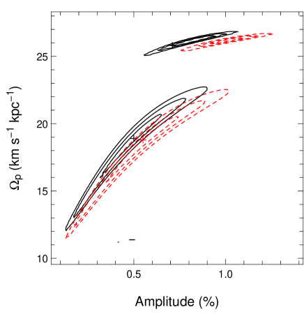
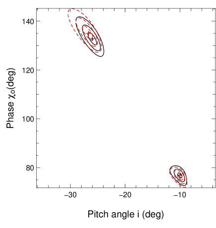
Figure 2: Cuts through the chi-square space around the best fit models in the amplitude vs pattern speed plane (left panel) and phase vs pitch angle plane (right panel). The crosses mark the location of the best fit while the contours are the 1, 2 and 3 $\sigma$ limits. The amplitude in the left panel is given as a percentage of the background potential at the Sun’s location. The plain lines are for the mass model I and the dashed lines for the mass model II. In both panels the top contours are for $m=4$, the bottom contours for $m=2$.

3.2 Resonances and spiral structure

The best fit $\,\langle V_{R}\rangle\,$velocity fields for the $m=2$ solutions using the mass models II is presented in Fig. 3. Although both reproduce equally well the structure of the velocity field between $y=\pm 1$ kpc, a small difference between the two solutions exists, model I predicting larger velocities in the top right and lower left corners of our sample (bottom right panel). However the velocity difference reaches only 0.2 $\mathrm{km\,s}^{-1}$, a level that lies below the capabilities of our data. The region below $y=-1$ kpc and at $0<x<1$ kpc is apprently poorly reproduced, however the lower left panel of Fig. 3 indicates that our solution stays well within the observational errors. The right panel of Fig. 1 indicates that this region suffers from large velocity errors and has therefore a lower weight in the solution. In the regions where our data are of the best quality (mostly $|y|<1$ kpc), our models reproduce adequately the observed velocity field.

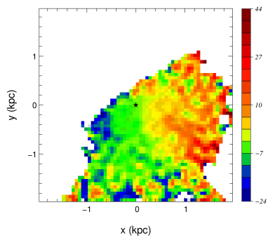
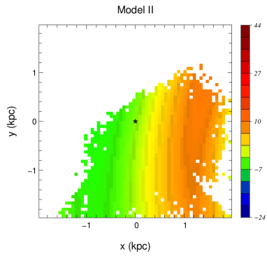
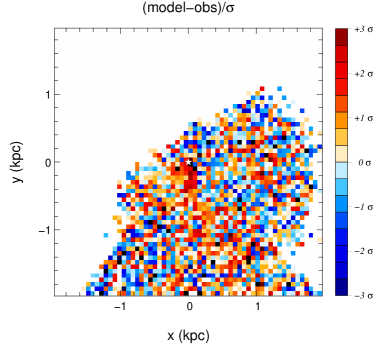
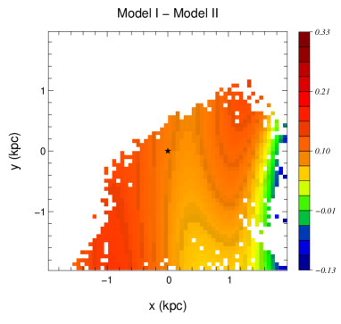
Figure 3: Top panels: observed velocity field (left) and model velocity field for the best fit solution using the mass model II (right). Bottom right: velocity field difference between the best fit solutions using the mass model I and II. The colour coding follows the median galactocentric radial velocity in $\mathrm{km\,s}^{-1}$in the three panels. Bottom left : difference $\langle V_{R,mII}\rangle-\langle V_{R,observed}\rangle$ normalised by the observational errors showing that all velocities on the 2 dimentional map are well recovered within the observational uncertainties. On all panels, the Sun’s location is at (0,0) and is marked by the black or white star.

Focusing on the pattern speed, our best models suggest that the Sun is located $\sim 200\,$pc inside the inner 4:1 resonance (ultra-harmonic renonance or UHR) of the spiral pattern (Fig. 4). Our finding for the pattern speed $\Omega_{p}=$18–19$\mathrm{km\,s}^{-1}\,\mathrm{kpc}^{-1}$is in agreement with recent studies that also place the Sun close to the UHR: $\Omega_{p}=17\,\mathrm{km\,s}^{-1}\,\mathrm{kpc}^{-1}\,$ by Antoja et al. (2011), $\Omega_{p}=18\,\mathrm{km\,s}^{-1}\,\mathrm{kpc}^{-1}\,$ by Quillen & Minchev (2005) or $\Omega_{p}/\Omega_{0}=0.65$ by Pompéia et al. (2011) to be compared to $\Omega_{p}/\Omega_{0}\sim 0.68$ in our study. However, as shown by Gerhard (2011), determinations of the spiral arms’ pattern speed range from 17 to 28 $\mathrm{km\,s}^{-1}\,\mathrm{kpc}^{-1}$, the higher values being prefered by open cluster birthplaces while hydrodynamical simulations and phase space substructures favour slower pattern speeds. It is interesting to note that the pattern speeds found from velocity space substructures (Quillen & Minchev 2005; Antoja et al. 2011; Pompéia et al. 2011) are close to our value. This would indicate a similar origin for the velocity gradient and the velocity substructures, reinforcing our assumption that the velocity gradient we observed is due to spiral arms. However this statement must be put in perspective as both types of study rely on the same assumptions that the spiral pattern is long-lived and tightly wound.

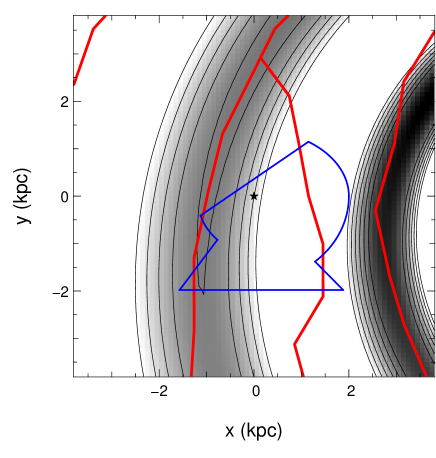
Figure 4: Left: circular frequency as a function of galactocentric distance for the mass model I of Binney & Tremaine (thick lines). The dotted and dashed lines are respectively the relations $\Omega\pm\kappa/4$ and $\Omega\pm\kappa/2$ versus R. The location of the Sun is marked by the vertical dotted line at $R_{0}=8\,\mathrm{kpc}\,$. The horizontal lines are the pattern speed corresponding to the best fit models for $m=2$ (plain lines) and $m=4$ (dash-dotted lines). Right: Density associated to the best model. The grey shading and contours represent the overdensity associated to the spiral perturbation. The contours are evenly spaced by $0.1\Sigma_{0}$, the background column density, from 0.1 to 0.5$\Sigma_{0}$. The blue contour depicts the footprint of the RAVE data. The red lines mark the location of the spiral arms in the gas from Englmaier et al. (2011). From left to right we have Cygnus arm (top left corner), the Perseus arm, the Sagittarius-Carina arm and the Scutum-Centaurus arm. The results for the mass model II are almost identical and are therefore not presented.

Comparing the predicted density pattern to the location of the spiral arms obtained by Englmaier et al. (2011) in the gas, we find a good agreement (Fig. 4 right panel). Both the Perseus arm and the Centaurus arm are recovered at the proper location. The Sagittarius-Carina arm is not recovered in our models. This indicates that this feature is not a dominant feature in the Solar neighborhood, reinforcing the view that the Milky Way spiral arm pattern is dominated by two main arms, Perseus and Centaurus (Drimmel 2000; Drimmel & Spergel 2001; Benjamin et al. 2005; Churchwell et al. 2009). Contrary to the $m=2$ models, our best fit $m=4$ solution does not reproduce any of the known spiral arms, in addition to being invalidated by its large pitch angle, hence an $m=2$ mode for the spiral pattern in the Milky Way is preferred within the Lin-Shu regime.

4 Conclusion

We have analysed the velocity gradient detected by Siebert et al. (2011a) using the RAVE data in the framework of the density wave model of Lin & Shu (1964), assuming that the velocity gradient we detected is due only to spiral arms and that the spiral arms in the Milky Way are long-lived.

Our model converges properly for an $m=2$ pattern, while if the chi-square of the $m=4$ solutions are comparable, the predicted pitch angle is too large, invalidating the solution.

The best fit solutions for $m=2$ reproduce adequately the observed velocity field for $\,\langle V_{R}\rangle\,$in the region $|y|<1$ kpc where our data are the most reliable. Outside of this region, the difference between the model and the observations is still within the observational errors although the agreement is less clear.

The predicted pattern speed places the Sun about 200 pc outside the inner UHR of the spiral arms. Such a location of the Sun is consistent with previous works based on velocity space substructures, suggesting a similar origin for the velocity space substructures and the $\,\langle V_{R}\rangle\,$gradient. Our best fit value for the amplitude of the spiral perturbation, $A=0.55^{+0.02}_{-0.02}\%$ of the background potential or 14% of the background density, is consistent with the value proposed by, e.g., Minchev & Famaey (2010) and is also in the range of earlier measurements as summarized in Antoja et al. (2011).

Comparing our model to the location of spiral arms in the gas, we find a good agreement with the location of the major spiral arms given by Englmaier et al. (2011). The density enhancement predicted by our best model matches the location of the Perseus and Centaurus arms. The Sagittarius arm is not reproduced by our solution which tends to reinforce previous studies concluding that the Milky Way spiral potential is dominated by a two-armed mode, the Sagittarius-Carina arm being a minor feature for the dynamics of the disc.

Our study relies on the density wave model of Lin & Shu (1964) and we assumed no vertical variation of the $\,\langle V_{R}\rangle\,$field within the limit of our data. RAVE data do contain the 3-dimensional spatial information which we will use in further studies. However, going from 2D to 3D requires an upgrade of our modeling technique taking properly into account the asymmetric drift and the vertical variation of the spiral potential. Moreover, vertical perturbations leading to possible variations of $\langle V_{z}\rangle(R,z)$ (Smith, Whiteoak & Evans 2012; Widrow et al. 2012; Williams et al. in prep.) are intrinsically not taken into account in our analysis. Future 3D simulations of such perturbations and their possible influence on the $\,\langle V_{R}\rangle\,$field will be necessary to disentangle their possible effects from the velocity gradient modeled here. Finally we note that our model is local as a result of the tight-winding approximation (see for example discussion in Binney 2012, Section 1.4.2). Ongoing surveys like Gaia-ESO (GES) or SDSS/SEGUE will provide data in the Galactic plane that can be used to test our models further in towards the Galactic centre (GES) or further out (SDSS/SEGUE). It will be interesting to test whether these two surveys predict the same pattern speed for the spiral arms.

References

- Adler & Wefstpfahl (1996) Adler D., Wefstpfahl D., 1996, AJ, 111, 735
- Antoja et al. (2011) Antoja T. et al., 2011, MNRAS, 418, 1423
- Benjamin et al. (2005) Benjamin R.A. et al., 2005, ApJ, 630, 149
- Bertin & Lin (1996) Bertin G., Lin C.C., 1996, Spiral Structure in Galaxies, Cambridge: The MIT Press
- Breddels et al. (2010) Breddels M.A. et al., 2010, A&A, 511, A90
- Binney et al. (1991) Binney J., Gerhard O., Stark A.A., Bally J., Uchida K.I., 1991, MNRAS, 252, 210
- Binney, Gerhard & Spergel (1997) Binney J., Gerhard O., Spergel D., 1997, MNRAS, 288, 365
- Binney (2012) Binney J., 2012, to appear in Falcon-Barroso J., Knapen J.H., eds, Secular Evolution of Galaxies (arXiv:1202.3403)
- Binney & Tremaine (2008) Binney J., Tremaine S., 2008, Galactic Dynamics, Princeton University Press.
- Bissantz et al. (2003) Bissantz N., Englmaier P., Gerhard O., 2003, MNRAS, 340, 949
- Burnett et al. (2011) Burnett B. et al., 2011, A&A, 532, A113
- Churchwell et al. (2009) Churchwell E. et al., 2009, PASP, 121, 213
- Dehnen (1998) Dehnen W., 1998, AJ, 115, 2384
- Dehnen & Binney (1998) Dehnen W., Binney J., 1998, MNRAS, 294, 429
- De Simone et al. (2004) De Simone R., Wu X., Tremaine S., 2004, MNRAS, 350, 627
- D’Onghia et al. (2012) D’Onghia E., et al., 2012, arXiv:1204.0513
- Drimmel (2000) Drimmel R., 2000, A&A, 358L, 13
- Drimmel & Spergel (2001) Drimmel R., Spergel D.N., 2001, ApJ, 556, 181
- Englmaier et al. (2011) Englmaier P., Pohl M., Bissantz N., 2011, Memorie della Societa Astronomica Italiana Supplement, 18,199
- Famaey et al. (2005) Famaey B., et al., 2005, A&A, 430, 165
- Foyle et al. (2011) Foyle K., et al., 2011, ApJ, 735, 101
- Georgelin & Georgelin (1976) Georgelin Y.M., Georgelin Y.P., 1976, A&A, 49, 57
- Gerhard (2011) Gerhard O., 2011, Mem. S.A.It. Suppl., 18, 185
- Grand et al. (2012a) Grand R.J.J., Kawata D., Cropper M., 2012, MNRAS, 421, 1529
- Grand et al. (2012b) Grand R.J.J., Kawata D., Cropper M., 2012, arXiv:1202.6387
- Kendall et al. (2008) Kendall S., et al., 2008, MNRAS, 387, 1007
- Lépine et al. (2011) Lépine J.R.D. et al., 2011, MNRAS, 417, 698
- Lépine et al. (2011b) Lépine J.R.D., Roman-Lopes A., Abraham Z., Junqueira T.C., Mishurov Y.N., 2011, MNRAS, 414, 1607
- Lin & Shu (1964) Lin C.C., Shu F.H., 1964, ApJ, 140, 646
- Lin, Yuan & Shu (1969) Lin C.C., Yuan C., Shu F.H., 1969, ApJ, 155, 721
- Lowe et al. (1994) Lowe S.A., et al., 1994, ApJ, 427, 184
- McMillan (2011) McMillan P. J., 2011, MNRAS, 418, 1565
- Minchev & Famaey (2010) Minchev I., Famaey B., 2010, ApJ, 722, 112
- Minchev et al. (2012) Minchev I., et al., 2012, arXiv:1203.2621
- Moni-Bidin, Carraro & Mendez (2012) Moni-Bidin C., Carraro G., Mendez R.A., 2012, ApJ, 747, 101
- Pilkington et al. (2012) Pilkington K., Gibson B. K., Jones D. H., 2012, arXiv1203.1996
- Pompéia et al. (2011) Pompéia L., et al., 2011, MNRAS, 415, 1138
- Quillen & Minchev (2005) Quillen A.C., Minchev I., 2005, AJ, 130, 576
- Quillen et al. (2011) Quillen A.C., Dougherty J., Bagley M. B., Minchev I., Comparetta J., 2011, MNRAS, 417, 762
- Reid et al. (2009) Reid M.J., et al., 2009, ApJ, 700, 137
- Salo et al. (2010) Salo H., et al., 2010, ApJ, 715, 56
- Schönrich et al. (2010) Schönrich R., Binney J., Dehnen W., 2010, MNRAS, 403, 1829
- Sellwood & Binney (2002) Sellwood J., Binney J., 2002, MNRAS, 336, 785
- Sellwood (2010a) Sellwood J., 2010, MNRAS, 410, 1637
- Sellwood (2010b) Sellwood, J., 2010, MNRAS, 409, 145
- Shaviv (2003) ShavivN.J., 2003, NewA, 8, 39
- Shetty (2007) Shetty R., et al., 2007, ApJ, 665, 1138
- Shu, Stachnik & Yost (1971) Shu F.H., Stachnik R.V., Yost J.C., 1971, ApJ 166, 465
- Siebert et al. (2008) Siebert A. et al., 2008, MNRAS, 391,793
- Siebert et al. (2011a) Siebert A. et al., 2011, MNRAS, 412,2026
- Siebert et al. (2011b) Siebert A. et al., 2011, AJ, 141,187
- Smith et al. (2009) Smith M.C. et al., 2009, MNRAS, 399, 1223
- Smith, Whiteoak & Evans (2012) Smith M.C., Whiteoak S. H., Evans N.W., 2012, ApJ, 746, 181
- Stanek et al. (1997) Stanek K.Z. et al., 1997, ApJ, 477, 163
- Steinmetz et al. (2006) Steinmetz M. et al., 2006, AJ, 132, 1645
- Struck et al. (2011) Struck C., Dobbs C.L., Hwang J.-S., 2011, MNRAS, 414, 2498
- Vallée (2008) Vallée J.P., 2008, AJ, 135, 1301
- Voglis et al. (2006) Voglis N., Stavropoulos I., Kalapotharakos C., 2006, MNRAS, 372, 901
- Widrow et al. (2012) Widrow L.M. et al., 2012, arXiv:1203.6861
- Williams et al. (in prep.) Williams M.E.K. et al., in preparation
- Zwitter et al. (2008) Zwitter T. et al., 2008, AJ, 136, 421
- Zwitter et al. (2010) Zwitter T. et al., 2010, A&A, 522A, 54