Abstract

We consider the integrable minimal models ${\cal M}(m,m^{\prime};t)$, corresponding to the $\varphi_{1,3}$ perturbation off-criticality, in the logarithmic limit  $m,m^{\prime}\to\infty$, $m/m^{\prime}\to p/p^{\prime}$ where $p,p^{\prime}$ are coprime and the limit is taken through coprime values of $m,m^{\prime}$. We view these off-critical minimal models ${\cal M}(m,m^{\prime};t)$ as the continuum scaling limit of the Forrester-Baxter Restricted Solid-On-Solid (RSOS) models on the square lattice. Applying Corner Transfer Matrices to the Forrester-Baxter RSOS models in Regime III, we argue that taking first the thermodynamic limit and second the logarithmic limit  yields off-critical logarithmic minimal models ${\cal LM}(p,p^{\prime};t)$ corresponding to the $\varphi_{1,3}$ perturbation of the critical logarithmic minimal models ${\cal LM}(p,p^{\prime})$. Specifically, in accord with the Kyoto correspondence principle, we show that the logarithmic limit of the one-dimensional configurational sums yields finitized quasi-rational characters of the Kac representations of the critical logarithmic minimal models ${\cal LM}(p,p^{\prime})$. We also calculate the logarithmic limit of certain off-critical observables ${\cal O}_{r,s}$ related to One Point Functions and show that the associated critical exponents $\beta_{r,s}=(2-\alpha)\,\Delta_{r,s}^{p,p^{\prime}}$ produce all conformal dimensions $\Delta_{r,s}^{p,p^{\prime}}<{(p^{\prime}-p)(9p-p^{\prime})\over 4pp^{\prime}}$ in the infinitely extended Kac table. The corresponding Kac labels $(r,s)$ satisfy $(ps-p^{\prime}r)^{2}<8p(p^{\prime}-p)$. The exponent $2-\alpha={p^{\prime}\over 2(p^{\prime}-p)}$ is obtained from the logarithmic limit of the free energy giving the conformal dimension $\Delta_{t}={1-\alpha\over 2-\alpha}={2p-p^{\prime}\over p^{\prime}}=\Delta_{1,3}^{p,p^{\prime}}$ for the perturbing field $t$. As befits a non-unitary theory, some observables ${\cal O}_{r,s}$ diverge at criticality.

1 Introduction

Consider the minimal models ${\cal M}(m,m^{\prime})$ [1] with coprime integers satisfying $2\leq m<m^{\prime}$. These are rational Conformal Field Theories (CFTs) with central charges

$$c=1-{6(m-m^{\prime})^{2}\over mm^{\prime}},\qquad 2\leq m<m^{\prime},\quad\mbox{$m,m^{\prime}$ coprime}$$ (1.1)

The conformal weights and their associated Virasoro characters are

$$\Delta_{r,s}^{m,m^{\prime}} ={(rm^{\prime}-sm)^{2}-(m-m^{\prime})^{2}\over 4mm^{\prime}},\quad 1\leq r\leq m-1,\ 1\leq s\leq m^{\prime}-1$$ (1.2)

$$\mbox{ch}^{m,m^{\prime}}_{r,s}(q) ={q^{-c/24+\Delta_{r,s}^{m,m^{\prime}}}\over(q)_{\infty}}\!\!\!\sum_{k=-\infty}^{\infty}\big{[}q^{k(kmm^{\prime}+rm^{\prime}-sm)}-q^{(km+r)(km^{\prime}+s)}\big{]}$$ (1.3)

where

$$(q)_{n}=\prod_{k=1}^{n}(1-q^{k}),\qquad(q)_{0}=1,\qquad(q)_{\infty}=\prod_{k=1}^{\infty}(1-q^{k})$$ (1.4)

In these expressions, $q=e^{\pi i\tau}$ is the modular nome.

The “logarithmic limit” [2] of the minimal CFTs is given symbolically by

$$\lim_{m,m^{\prime}\to\infty,\ {m\over m^{\prime}}\to{p\over p^{\prime}}}{\cal M}(m,m^{\prime})={\cal LM}(p,p^{\prime}),\qquad 1\leq p<p^{\prime},\quad\mbox{$p,p^{\prime}$ coprime}$$ (1.5)

where the limit is taken through coprime pairs $(m,m^{\prime})$. Since $p\geq 1$, the limit must ultimately be taken through a sequence of non-unitary models with $m\neq m^{\prime}-1$. Here ${\cal LM}(p,p^{\prime})$ denotes the logarithmic minimal models [3]. The limit is taken directly in the continuum scaling limit, after the thermodynamic limit. The equality indicates the identification of the spectra of these CFTs. In principle, the Jordan cells appearing in the reducible yet indecomposable representations of the logarithmic minimal models should emerge in this limit but there are subtleties [2]. Here we only consider the limit of spectra for which purpose the logarithmic limit is robust in the sense that it is independent of the choice of the sequence.

Taking the logarithmic limit of the conformal data of the rational minimal models ${\cal M}(m,m^{\prime})$ yields directly [2] the conformal data of the logarithmic minimal models ${\cal LM}(p,p^{\prime})$

$$\begin{array}[]{rcll}\displaystyle c&\!\!=\!\!&\displaystyle 1-{6(p-p^{\prime})^{2}\over pp^{\prime}},&1\leq p<p^{\prime},\quad\ \ \mbox{$p,p^{\prime}$ coprime}\\[12.0pt] \displaystyle\Delta_{r,s}^{p,p^{\prime}}&\!\!=\!\!&\displaystyle{(rp^{\prime}-sp)^{2}-(p-p^{\prime})^{2}\over 4pp^{\prime}},&r=1,2,\ldots;\ s=1,2,\ldots\\[12.0pt] \chi^{p,p^{\prime}}_{r,s}(q)&\!\!=\!\!&\displaystyle q^{-c/24+\Delta_{r,s}^{p,p^{\prime}}}{(1-q^{rs})\over(q)_{\infty}},&r=1,2,\ldots;\ s=1,2,\ldots\end{array}$$ (1.9)

The logarithmic characters are the quasi-rational characters of the so-called Kac representations which are organized into infinitely extended Kac tables. The Kac tables of conformal weights for critical dense polymers ${\cal LM}(1,2)$ and critical percolation ${\cal LM}(2,3)$ are shown in Table 1.

Table 1: Infinitely extended Kac tables of conformal weights $\Delta_{r,s}^{p,p^{\prime}}$ for critical dense polymers ${\cal LM}(1,2)$ and critical percolation ${\cal LM}(2,3)$. The positions corresponding to irreducible representations are marked with a quadrant in the top-right corner. The boxes of the conformal dimensions $\Delta_{r,s}<{(p^{\prime}-p)(9p-p^{\prime})\over 4pp^{\prime}}$ that are accessible, using Corner Transfer Matrices to calculate off-critical observables, are shaded in pink and occur in the band where $(r,s)$ satisfy $(ps-p^{\prime}r)^{2}<8p(p^{\prime}-p)$.

Figure 1: Commutative diagram of the logarithmic limit and $\varphi_{1,3}$ off-critical perturbation.

In this paper, we consider the logarithmic limit of the off-critical minimal models and argue that it provides an integrable off-critical perturbation of the logarithmic minimal models. We denote the off-critical models by ${\cal M}(m,m^{\prime};t)$ or ${\cal M}(m,m^{\prime};q)$ where $t=e^{-\epsilon}$ and $q=e^{-4\pi^{2}(m^{\prime}-m)/m^{\prime}\epsilon}$ are conjugate off-critical nomes measuring the temperature. Symbolically, as in Figure 1, we write

$$\lim_{m,m^{\prime}\to\infty,\ {m\over m^{\prime}}\to{p\over p^{\prime}}}{\cal M}(m,m^{\prime};t)={\cal LM}(p,p^{\prime};t),\qquad 1\leq p<p^{\prime},\quad\mbox{$p,p^{\prime}$ coprime}$$ (1.10)

where now $t$ is an elliptic nome measuring the departure from criticality. Since degeneracies necessary for the formation of Jordan cells are lifted off-criticality, the off-critical logarithmic minimal models are not expected to exhibit the logarithmic structures, such as reducible yet indecomposable representations, associated with logarithmic CFTs. Nevertheless, we call these models off-critical logarithmic minimal models to emphasize their relation to their logarithmic critical counterparts. Notice that although ${\cal LM}(2,3)={\cal LM}(2,3;0)$ is critical bond percolation, the integrable off-critical percolation model ${\cal LM}(2,3;t)$ does not coincide with the off-critical bond percolation model. To put it another way, as shown in Appendix A, the off-critical model ${\cal LM}(2,3;t)$ is the integrable $\varphi_{1,3}$ perturbation of critical bond percolation

$$\Delta_{t}=\frac{1-\alpha}{2-\alpha}=\frac{1}{3}=\Delta_{1,3}^{2,3},\qquad t\sim\varphi_{1,3}$$ (1.11)

In contrast, the usual off-critical bond percolation model [4] corresponds to a $\varphi_{2,1}$ perturbation. The (mean cluster number) critical exponent is $\alpha_{p}=-\frac{2}{3}$ corresponding to the off-critical $\varphi_{2,1}$ perturbation

$$\Delta_{p}=\frac{1-\alpha_{p}}{2-\alpha_{p}}=\frac{5}{8}=\Delta_{2,1}^{2,3},\qquad p\sim\varphi_{2,1}$$ (1.12)

where here $p$ is the bond occupation probability with $p_{c}=\mbox{$\textstyle\frac{1}{2}$}$ [5].

The content of the paper is as follows. It is known that the rational minimal models are described by the continuum scaling limit of the Forrester-Baxter RSOS models [6, 7] in Regime III. In Section 2, we use Corner Transfer Matrix (CTM) techniques to study the logarithmic limit of the one-dimensional configurational sums of the Forrester-Baxter RSOS models in Regime III. We show that, up to the leading terms involving the central charges and conformal dimensions, the one-dimensional configurational sums reproduce the finitized quasi-rational Kac character formulas. This observation is in agreement with the general correspondence principle of the Kyoto school [8] which is valid in Regime III. In Section 3, we obtain general expressions for the One Point Functions (OPFs), first for the Forrester-Baxter models and then in the logarithmic limit. We extract critical exponents from the behaviour of suitably defined Generalized Order Parameters near the critical point $t\to 0$. In the logarithmic limit, these exponents are simply related to conformal dimensions in the infinitely extended Kac table. In Appendix A, we look at the behaviour of the logarithmic limit of the free energy as $t\to 0$ and argue that the relevant perturbation, away from the critical logarithmic minimal models, is the thermal $\varphi_{1,3}$ perturbation. In Appendix B, we collect relevant properties of elliptic functions.

2 1-$d$ Configurational Sums of Limiting Forrester-Baxter Models

2.1 Forrester-Baxter models

The Forrester-Baxter RSOS lattice models [7] are defined on a square lattice with heights $a=1,2,\ldots,m^{\prime}-1$ restricted so that nearest neighbour heights differ by $\pm 1$. The heights thus live on the $A_{m^{\prime}-1}$ Dynkin diagram. The Boltzmann weights are

$$W\!\!\left.\left(\begin{matrix}a\pm 1&a\\ a&a\mp 1\end{matrix}\right|u\right)=\frac{s(\lambda-u)}{s(\lambda)}\ \ \ \ \begin{pspicture}[missing](0.0pt,-7.0pt)(28.0pt,35.0pt){\psset{linewidth=0.5pt,fillstyle=solid,fillcolor=lightlightblue}\pspolygon(0.0pt,0.0pt)(28.0pt,0.0pt)(28.0pt,28.0pt)(0.0pt,28.0pt)(0.0pt,0.0pt)}\rput[tr](0.0pt,0.0pt){\scriptsize$a$}\rput[tl](28.0pt,0.0pt){\scriptsize$a\!\mp\!1$}\rput[bl](28.0pt,28.0pt){\scriptsize$a$}\rput[br](0.0pt,28.0pt){\scriptsize$a\!\pm\!1$}\end{pspicture}\ \;=\ \;\frac{s(\lambda-u)}{s(\lambda)}\ \ \ \ \begin{pspicture}[missing](0.0pt,-7.0pt)(28.0pt,35.0pt){\psset{linewidth=0.5pt,fillstyle=solid,fillcolor=lightlightblue}\pspolygon(0.0pt,0.0pt)(28.0pt,0.0pt)(28.0pt,28.0pt)(0.0pt,28.0pt)(0.0pt,0.0pt)}\rput[tr](0.0pt,0.0pt){\scriptsize$a$}\rput[tl](28.0pt,0.0pt){\scriptsize$a\!\mp\!1$}\rput[bl](28.0pt,28.0pt){\scriptsize$a$}\rput[br](0.0pt,28.0pt){\scriptsize$a\!\pm\!1$}{\psset{linewidth=0.5pt}\psarc(0.0pt,28.0pt){14.0pt}{270.0}{0.0}}{\psset{linewidth=0.5pt}\psarc(28.0pt,0.0pt){14.0pt}{90.0}{180.0}}{\psset{linewidth=1.0pt,linecolor=blue}\psline(0.0pt,0.0pt)(28.0pt,28.0pt)}\end{pspicture}$$ (2.1)

$$W\!\!\left.\left(\begin{matrix}a&a\pm 1\\ a\mp 1&a\end{matrix}\right|u\right)={g_{a\mp 1}\over g_{a\pm 1}}\,\frac{s((a\pm 1)\lambda)}{s(a\lambda)}\,\frac{s(u)}{s(\lambda)}\ \ \ \ \ \begin{pspicture}[missing](0.0pt,-7.0pt)(28.0pt,35.0pt){\psset{linewidth=0.5pt,fillstyle=solid,fillcolor=lightlightblue}\pspolygon(0.0pt,0.0pt)(28.0pt,0.0pt)(28.0pt,28.0pt)(0.0pt,28.0pt)(0.0pt,0.0pt)}\rput[tr](0.0pt,0.0pt){\scriptsize$a\!\mp\!1$}\rput[tl](28.0pt,0.0pt){\scriptsize$a$}\rput[bl](28.0pt,28.0pt){\scriptsize$a\!\pm\!1$}\rput[br](0.0pt,28.0pt){\scriptsize$a$}\end{pspicture}\ \;=\ \;{g_{a\mp 1}\over g_{a\pm 1}}\,\frac{s((a\pm 1)\lambda)}{s(a\lambda)}\,\frac{s(u)}{s(\lambda)}\ \ \;\ \ \begin{pspicture}[missing](0.0pt,-7.0pt)(28.0pt,35.0pt){\psset{linewidth=0.5pt,fillstyle=solid,fillcolor=lightlightblue}\pspolygon(0.0pt,0.0pt)(28.0pt,0.0pt)(28.0pt,28.0pt)(0.0pt,28.0pt)(0.0pt,0.0pt)}\rput[tr](0.0pt,0.0pt){\scriptsize$a\!\mp\!1$}\rput[tl](28.0pt,0.0pt){\scriptsize$a$}\rput[bl](28.0pt,28.0pt){\scriptsize$a\!\pm\!1$}\rput[br](0.0pt,28.0pt){\scriptsize$a$}{\psset{linewidth=0.5pt}\psarc(0.0pt,0.0pt){14.0pt}{0.0}{90.0}}{\psset{linewidth=0.5pt}\psarc(28.0pt,28.0pt){14.0pt}{180.0}{270.0}}{\psset{linewidth=1.0pt,linecolor=blue}\psline(0.0pt,28.0pt)(28.0pt,0.0pt)}\end{pspicture}$$ (2.2)

$$W\!\!\left.\left(\begin{matrix}a&a\pm 1\\ a\pm 1&a\end{matrix}\right|u\right)=\frac{s(a\lambda\pm u)}{s(a\lambda)}\ \;\ \ \begin{pspicture}[missing](0.0pt,-7.0pt)(28.0pt,35.0pt){\psset{linewidth=0.5pt,fillstyle=solid,fillcolor=lightlightblue}\pspolygon(0.0pt,0.0pt)(28.0pt,0.0pt)(28.0pt,28.0pt)(0.0pt,28.0pt)(0.0pt,0.0pt)}\rput[tr](0.0pt,0.0pt){\scriptsize$a\!\pm\!1$}\rput[tl](28.0pt,0.0pt){\scriptsize$a$}\rput[bl](28.0pt,28.0pt){\scriptsize$a\!\pm\!1$}\rput[br](0.0pt,28.0pt){\scriptsize$a$}\end{pspicture}$$

$$\quad=\;{c(0)c((a\!\pm\!1)\lambda\!\pm\!u)\over c((a\!\pm\!1)\lambda)c(u)}{s(\lambda\!-\!u)\over s(\lambda)}\ \;\ \ \begin{pspicture}[missing](0.0pt,-7.0pt)(28.0pt,35.0pt){\psset{linewidth=0.5pt,fillstyle=solid,fillcolor=lightlightblue}\pspolygon(0.0pt,0.0pt)(28.0pt,0.0pt)(28.0pt,28.0pt)(0.0pt,28.0pt)(0.0pt,0.0pt)}\rput[tr](0.0pt,0.0pt){\scriptsize$a\!\pm\!1$}\rput[tl](28.0pt,0.0pt){\scriptsize$a$}\rput[bl](28.0pt,28.0pt){\scriptsize$a\!\pm\!1$}\rput[br](0.0pt,28.0pt){\scriptsize$a$}{\psset{linewidth=0.5pt}\psarc(0.0pt,28.0pt){14.0pt}{270.0}{0.0}}{\psset{linewidth=0.5pt}\psarc(28.0pt,0.0pt){14.0pt}{90.0}{180.0}}{\psset{linewidth=1.0pt,linecolor=blue}\psline(0.0pt,0.0pt)(28.0pt,28.0pt)}\end{pspicture}\ \;+{c(\lambda)c(a\lambda\!\pm\!u)\over c((a\!\pm\!1)\lambda)c(u)}{s((a\!\pm\!1)\lambda)\over s(a\lambda)}\,{s(u)\over s(\lambda)}\ \ \;\ \ \begin{pspicture}[missing](0.0pt,-7.0pt)(28.0pt,35.0pt){\psset{linewidth=0.5pt,fillstyle=solid,fillcolor=lightlightblue}\pspolygon(0.0pt,0.0pt)(28.0pt,0.0pt)(28.0pt,28.0pt)(0.0pt,28.0pt)(0.0pt,0.0pt)}\rput[tr](0.0pt,0.0pt){\scriptsize$a\!\pm\!1$}\rput[tl](28.0pt,0.0pt){\scriptsize$a$}\rput[bl](28.0pt,28.0pt){\scriptsize$a\!\pm\!1$}\rput[br](0.0pt,28.0pt){\scriptsize$a$}{\psset{linewidth=0.5pt}\psarc(0.0pt,0.0pt){14.0pt}{0.0}{90.0}}{\psset{linewidth=0.5pt}\psarc(28.0pt,28.0pt){14.0pt}{180.0}{270.0}}{\psset{linewidth=1.0pt,linecolor=blue}\psline(0.0pt,28.0pt)(28.0pt,0.0pt)}\end{pspicture}$$ (2.3)

Here $s(u)=\vartheta_{1}(u,t)$ and $c(u)=\vartheta_{4}(u,t)$ are standard elliptic theta functions [9] as in Appendix B, $u$ is the spectral parameter and the elliptic nome $t=e^{-\epsilon}$ is a temperature-like variable, with $t^{2}$ measuring the departure from criticality corresponding to the $\varphi_{1,3}$ integrable perturbation. The gauge factors $g_{a}$ are inessential and can be set either to $1$ or $g_{a}=\sqrt{s(a\lambda)}$, as in [7], to restore reflection symmetry. The crossing parameter $\lambda$ is

$$\lambda={(m^{\prime}-m)\pi\over m^{\prime}},\qquad 2\leq m<m^{\prime},\qquad\mbox{$m,m^{\prime}$ coprime}$$ (2.4)

The RSOS faces are decomposed into decorated faces or tiles (2-tangles) of the planar algebra [10] having height degrees of freedom at the corners and twofold internal degrees of freedom associated with the direction of the loop segments, or equivalently, the diagonal bonds. These models can be viewed as generalized models of polymers and percolation with percolation properties described in terms of percolating loops or percolating bond clusters. Sites in a common bond cluster share a common height $a$. Integrability derives from the fact that the local face weights satisfy the Yang-Baxter equation [11]. In the symmetric gauge, the face weights also obey the crossing symmetry

$$W\!\!\left.\left(\begin{matrix}d&c\\ a&b\end{matrix}\right|\lambda-u\right)=\sqrt{\frac{s(a\lambda)s(c\lambda)}{s(b\lambda)s(d\lambda)}}\,W\!\!\left.\left(\begin{matrix}c&b\\ d&a\end{matrix}\right|u\right)$$ (2.5)

At criticality and in the symmetric gauge, the Boltzmann weights reduce to

$$W\!\!\left.\left(\begin{matrix}d&c\\ a&b\end{matrix}\right|u\right)=\;{s(\lambda\!-\!u)\over s(\lambda)}\,\delta_{a,c}\;+\sqrt{{s(a\lambda)s(c\lambda)\over s(b\lambda)s(d\lambda)}}\,{s(u)\over s(\lambda)}\,\delta_{b,d}$$ (2.6)

with $s(u)=\sin u$. The height dependent square root factors give rise to a matrix representation [12] of the Temperley-Lieb [13] generators $e_{j}$ acting on paths built on the graph $A_{m^{\prime}-1}$. It follows that the associated face operators are

$$X_{j}(u)={s(\lambda\!-\!u)\over s(\lambda)}\,I+{s(u)\over s(\lambda)}\,e_{j}$$ (2.7)

where $I$ is the identity matrix. The Temperley-Lieb generators satisfy $e_{j}^{2}=\beta e_{j}$ where the loop fugacity $\beta=2\cos{(m^{\prime}-m)\pi\over m^{\prime}}\to 2\cos{(p^{\prime}-p)\pi\over p^{\prime}}$ in the logarithmic limit. The face operators (2.7) thus coincide with those of the logarithmic minimal models ${\cal LM}(p,p^{\prime})$ except that in [3] the loop representation is used as opposed to the height representation of the Temperley-Lieb algebra used in this paper. On the strip, it is possible to construct a Markov trace [14] on the Temperley-Lieb algebra such that the traces of words in the algebra are independent of the choice of representation. It follows that, if we use this Markov trace on the strip, the resulting partition functions for the logarithmic theories ${\cal LM}(p,p^{\prime})$ will agree with the logarithmic limit of the partition functions of the RSOS theories (2.6).

It does not make sense to take the logarithmic limit (1.10) of the face weights directly because the factors $s(a\lambda)$ vanish whenever $a$ is a multiple of $p^{\prime}$ causing some weights to vanish and others to diverge. To avoid this problem, we take the logarithmic limit after the thermodynamic limit. In practice, however, quantities for ${\cal LM}(p,p^{\prime};t)$ can be obtained within arbitrary precision by considering a non-unitary minimal model with Boltzmann weights (2.1)–(2.3) and judiciously choosing the crossing parameter, say $\lambda=2,000,000\,\pi/3,000,001$ for off-critical percolation.

Figure 2: Square lattice geometry for Corner Transfer Matrices $A,B,C,D$. The half-row configurations are given by $\sigma=\{\sigma_{0},\sigma_{1},\sigma_{2},\ldots,\sigma_{N},\sigma_{N+1}\}$ with the boundary conditions $\sigma_{N}=\tilde{b}$ and $\sigma_{N+1}=\tilde{c}$ with $\tilde{b},\tilde{c}=1,2,\ldots,m^{\prime}-1$ and $\tilde{b}-\tilde{c}=\pm 1$. The center height $\sigma_{0}=1,2,\ldots,m^{\prime}-1$ is fixed to the value $s$ by the diagonal matrix $S$ with entries $\langle\sigma|S|\sigma^{\prime}\rangle=\delta(\sigma_{0},s)\prod_{j=0}^{N+1}\delta(\sigma_{j},\sigma_{j}^{\prime})$. The condition $N+s-\tilde{b}=0$ mod 2 ensures that it is possible to get from $s$ to $\tilde{b}$ in $N$ steps. Internal heights, shown with a solid disk, are summed over. The groundstate boundary conditions are labelled by $r=1,2,\ldots,m-1$. If $N+s-b=0$ mod 2, the boundary heights are fixed as shown with $\tilde{b}=b=b(r)=\lfloor{rm^{\prime}\over m}\rfloor$ and $\tilde{c}=b+1$. Otherwise, if $N+s-b=1$ mod 2, the boundary heights are $\tilde{b}=b+1$ and $\tilde{c}=b=b(r)$. In both cases, $b=b(r)=\mbox{Min}[\tilde{b},\tilde{c}]$.

2.2 Corner transfer matrices and 1-dimensional configurational sums

The one-dimensional configurational sums [11] arise from the diagonalization of the Corner Transfer Matrices (CTMs) of Figure 2. Allowing for translations, the Forrester-Baxter models admit $2(m-1)$ groundstates in Regime III wherein the heights outside of the finite region shown in Figure 2 alternate between $b$ and $b+1$ on the two sublattices of the square lattice. The allowed values of $b$ are

$$b=b(r)=\big{\lfloor}{rm^{\prime}\over m}\big{\rfloor},\qquad r=1,2,\ldots,m-1$$ (2.8)

with inverse

$$r=r(b)=\big{\lfloor}{b\,m\over m^{\prime}}\big{\rfloor}+1$$ (2.9)

In a given sector, specified by the boundary conditions $(\sigma_{0},\sigma_{N},\sigma_{N+1})$, the eigenvalues of the CTMs are labelled by paths $\sigma$ on the $A_{m^{\prime}-1}$ diagram that start at $\sigma_{0}=a$ and end with either $\sigma_{N}=b$, $\sigma_{N+1}=b+1$ or $\sigma_{N}=b+1$, $\sigma_{N+1}=b$. We denote this set of paths by ${\cal P}_{a\tilde{b}\tilde{c}}^{m^{\prime}}(N)$ or just ${\cal P}_{abc}^{m^{\prime}}(N)$ when $b,c$ are generic dummy heights which should not cause confusion with the groundstate labels $b=b(r)$. A typical path with the groundstate bands $(b,b+1)$ shaded is shown in Figure 3. More precisely, the one-dimensional configurational sums are given by

$$X_{abc}^{(N)}(q)\!=\!\displaystyle\sum_{\sigma}q^{\sum_{j=1}^{N}jH(\sigma_{j-1},\sigma_{j},\sigma_{j+1})-E_{0}},\quad\sigma\!=\!\{\sigma_{0},\sigma_{1},\ldots,\sigma_{N},\sigma_{N+1}\}\in{\cal P}_{abc}^{m^{\prime}}(N)$$ (2.10)

subject to the boundary conditions

$$(\sigma_{0},\sigma_{N},\sigma_{N+1})\!=\!(a,b,c)$$ (2.11)

where the local energy function is

$$H(a,a\mp 1,a)=\pm\big{\lfloor}{a(m^{\prime}-m)\over m^{\prime}}\big{\rfloor},\qquad H(a-1,a,a+1)=H(a+1,a,a-1)=\mbox{$\textstyle\frac{1}{2}$}$$ (2.12)

As a consequence of the crossing symmetry (2.5), the conjugate nome in the one-dimensional configurational sums (2.10) is $q=e^{-4\pi\lambda/\epsilon}$ with the original nome of the face weights given by $t=e^{-\epsilon}$. The constant $E_{0}$ is the energy of the path with minimum energy. Its presence ensures that the $q$-series begins as $1+O(q)$. Explicitly, the ground state energy for boundary conditions (2.11) is

$$E_{0}={1\over 4}(a-b)(a-c)+{1\over 2}\big{[}(a-c)+(c-b)(N+1)\big{]}\big{\lfloor}\frac{c(m^{\prime}-m)}{m^{\prime}}\big{\rfloor}$$ (2.13)

The one-dimensional configurational sums are purely combinatorial objects [15]. They are the energy generating functions for the CTM eigenvalues.

Figure 3: The path $\sigma=\{1,2,3,4,5,4,5,4,5,4,5\}$ of ${\cal M}(5,8;q)$ on $A_{7}$ with length $N=9$ and boundary condition $(\sigma_{0},\sigma_{N},\sigma_{N+1})=(1,4,5)=(s,b,b+1)$. The groundstate bands $(b,b+1)$ at $b=b(r)=\big{\lfloor}{rm^{\prime}\over m}\big{\rfloor}=1,3,4,6$ are shown shaded. This is the path with minimum energy $E_{0}=6$ in the $(r,s)=(3,1)$ sector since $b(3)=4$.

The one-dimensional configurational sums can be evaluated [7] by solving recursion equations subject to appropriate initial conditions. Explicitly, for the Forrester-Baxter models, the solutions are

$$\begin{array}[]{rcl}X_{ab\{b+1\}}^{(N)}(q)&\!\!\!\!=\!\!\!\!&\displaystyle\sum_{k=-\infty}^{\infty}\!\!\Big{(}q^{k(kmm^{\prime}+rm^{\prime}-am)}\Big{[}\!\!\begin{array}[]{c}{N}\\ {{N+a-b\over 2}-km^{\prime}}\end{array}\!\!\Big{]}-q^{(km+r)(km^{\prime}+a)}\Big{[}\!\!\begin{array}[]{c}{N}\\ {{N-a-b\over 2}-km^{\prime}}\end{array}\!\!\Big{]}\Big{)}\\[18.0pt] X_{a\{b+1\}b}^{(N)}(q)&\!\!\!\!=\!\!\!\!&\displaystyle\sum_{k=-\infty}^{\infty}\!\!\!\Big{(}q^{k(kmm^{\prime}+rm^{\prime}-am)}\Big{[}\!\!\begin{array}[]{c}{N}\\ {{N+a-b-1\over 2}-km^{\prime}}\end{array}\!\!\Big{]}-q^{(km+r)(km^{\prime}+a)}\Big{[}\!\!\begin{array}[]{c}{N}\\ {{N-a-b-1\over 2}-km^{\prime}}\end{array}\!\!\Big{]}\Big{)}\end{array}$$ (2.24)

for the two mod $2$ parities of $N+a-b$ where $b=1,2,\ldots,m-2$. The $q$-binomials appearing in these formulas are defined by

$$\Big{[}\!\!\begin{array}[]{c}{m+n}\\ {m}\end{array}\!\!\Big{]}=\begin{cases}\dfrac{(q)_{m+n}}{(q)_{m}(q)_{n}},&\quad m,n\geq 0\\[4.0pt] 0,&\quad\text{otherwise}\\ \end{cases}$$ (2.27)

The one-dimensional configurational sums coincide with finitized Virasoro characters

$$\mbox{ch}^{(N)}_{r,s}(q)=\begin{cases}q^{-c/24+\Delta_{r,s}^{m,m^{\prime}}}X_{sb\{b+1\}}^{(N)}(q),&b=b(r),\quad N+s-b=0\ \mbox{mod 2}\\[6.0pt] q^{-c/24+\Delta_{r,s}^{m,m^{\prime}}}X_{s\{b+1\}b}^{(N)}(q),&b=b(r),\quad N+s-b=1\ \mbox{mod 2}\end{cases}$$ (2.28)

where $q$ is now the modular nome and

$$\lim_{N\to\infty}\mbox{ch}^{(N)}_{r,s}(q)=\mbox{ch}^{m,m^{\prime}}_{r,s}(q),\qquad r=1,2,\ldots,m-1;\quad s=1,2,\ldots,m^{\prime}-1$$ (2.29)

2.3 Logarithmic limit of Forrester-Baxter models

In the logarithmic limit, the heights $\sigma_{j}$ are unrestricted and live on the (one-sided) $A_{\infty}$ diagram. Notice however that, for given boundary conditions and any fixed $N$, the heights can only assume a finite range of values. In this limit, the banding pattern is repeated periodically with period $p^{\prime}$. Explicitly, the groundstate bands $(b,b+1)$ are given by

$$b=b(r)=\big{\lfloor}{rp^{\prime}\over p}\big{\rfloor},\qquad r=1,2,3,\ldots$$ (2.30)

For the ${\cal LM}(1,p^{\prime};q)$ theories, the groundstate bands are simply $b(r)=p^{\prime}r$. For off-critical logarithmic dense polymers ${\cal LM}(1,2;q)$, percolation ${\cal LM}(2,3;q)$ and Lee-Yang ${\cal LM}(2,5;q)$ the groundstate bands are located at

$$b(r)=\begin{cases}2,4,6,8,10,12,\ldots&(p,p^{\prime})=(1,2)\\ 1,3,4,6,7,9,10,12\ldots&(p,p^{\prime})=(2,3)\\ 2,5,7,10,12,15,17,20,\ldots&(p,p^{\prime})=(2,5)\end{cases}\qquad r=1,2,3,\ldots$$ (2.31)

The one-dimensional configurational sums give a finite set of eigenvalues of the infinite system. The $N$ in these formulas is a truncation size and not the system size which has already been taken to infinity. We can therefore apply the logarithmic limit directly to the one-dimensional configurational sums.

The unrestricted one-dimensional configurational sums are given by

$$Y_{abc}^{(N)}(q)\!=\!\sum_{\sigma}q^{\sum_{j=1}^{N}jH^{\infty}(\sigma_{j-1},\sigma_{j},\sigma_{j+1})-E_{0}^{\infty}},\quad\sigma\!=\!\{\sigma_{0},\sigma_{1},\ldots,\sigma_{N},\sigma_{N+1}\}\in{\cal P}_{abc}^{\infty}(N)$$ (2.32)

subject to the boundary conditions (2.11) with local energy function

$$H^{\infty}(a,a\mp 1,a)=\pm\big{\lfloor}{a(p^{\prime}-p)\over p^{\prime}}\big{\rfloor},\qquad H^{\infty}(a-1,a,a+1)=H^{\infty}(a+1,a,a-1)=\mbox{$\textstyle\frac{1}{2}$}$$ (2.33)

Taking the logarithmic limit of the Forrester-Baxter results (2.24), gives

$$\begin{array}[]{rcl}Y_{ab\{b+1\}}^{(N)}(q)&\!\!=\!\!&\displaystyle\Big{[}\!\!\begin{array}[]{c}{N}\\ {{N+a-b\over 2}}\end{array}\!\!\Big{]}-q^{ra}\Big{[}\!\!\begin{array}[]{c}{N}\\ {{N-a-b\over 2}}\end{array}\!\!\Big{]},\qquad\qquad N+a-b=0\ \mbox{mod 2}\\[10.0pt] Y_{a\{b+1\}b}^{(N)}(q)&\!\!=\!\!&\displaystyle\Big{[}\!\!\begin{array}[]{c}{N}\\ {{N+a-b-1\over 2}}\end{array}\!\!\Big{]}-q^{ra}\Big{[}\!\!\begin{array}[]{c}{N}\\ {{N-a-b-1\over 2}}\end{array}\!\!\Big{]},\qquad N+a-b=1\ \mbox{mod 2}\end{array}$$ (2.44)

In accord with the Kyoto correspondence principle [8], these one-dimensional configurational sums coincide with finitized quasi-rational characters of the Kac representations of the critical ${\cal LM}(p,p^{\prime})$ models

$$\chi^{(N)}_{r,s}(q)=\begin{cases}q^{-c/24+\Delta_{r,s}^{p,p^{\prime}}}Y_{sb\{b+1\}}^{(N)}(q),&b=b(r),\quad N+s-b=0\ \mbox{mod 2}\\[6.0pt] q^{-c/24+\Delta_{r,s}^{p,p^{\prime}}}Y_{s\{b+1\}b}^{(N)}(q),&b=b(r),\quad N+s-b=1\ \mbox{mod 2}\end{cases}$$ (2.45)

with

$$\lim_{N\to\infty}\chi^{(N)}_{r,s}(q)=\chi^{p,p^{\prime}}_{r,s}(q),\qquad r,s=1,2,3,\ldots$$ (2.46)

Again $q$ is the modular nome in these character formulas. An alternative view is that, in Regime III, the massive-conformal renormalization group flow is uninteresting. In the words of Melzer [16], there exists a simple massive-conformal dictionary between eigenstates. This is not the case in Regime IV.

We note that the one-dimensional configurational sums of the logarithmic theory

$$\bar{Y}_{abc}^{(N)}(q)=q^{E_{0}^{\infty}}Y_{abc}^{(N)}(q)$$ (2.47)

satisfy [17] CTM recursions of the usual form

$$\begin{array}[]{rcl}\bar{Y}_{ab\{b+1\}}^{(N)}(q)\!\!&=&\!\!q^{N\lfloor{(b+1)(p^{\prime}-p)\over p^{\prime}}\rfloor}\bar{Y}_{a\{b+1\}b}^{(N-1)}(q)+q^{N\over 2}\bar{Y}_{a\{b-1\}b}^{(N-1)}(q)\\[6.0pt] \bar{Y}_{ab\{b-1\}}^{(N)}(q)\!\!&=&\!\!q^{N\over 2}\bar{Y}_{a\{b+1\}b}^{(N-1)}(q)+q^{-N\lfloor{(b-1)(p^{\prime}-p)\over p^{\prime}}\rfloor}\bar{Y}_{a\{b-1\}b}^{(N-1)}(q)\end{array}$$ (2.50)

subject to the initial and boundary conditions

$$\bar{Y}_{abc}^{(0)}(q)=\delta_{a,b},\qquad\bar{Y}_{a\{0\}1}^{(N)}(q)=0$$ (2.51)

Here the groundstate energy $E_{0}^{\infty}$ for walks on $A^{\infty}$ is the logarithmic limit of the expression for $E_{0}$

$$E_{0}^{\infty}={1\over 4}(a-b)(a-c)+{1\over 2}\big{[}(a-c)+(c-b)(N+1)\big{]}\big{\lfloor}\frac{c(p^{\prime}-p)}{p^{\prime}}\big{\rfloor},\quad(\sigma_{0},\sigma_{N},\sigma_{N+1})=(a,b,c)$$ (2.52)

3 One-Point Functions of the Forrester-Baxter Models

In this section we discuss the One Point Functions (OPFs) and Generalized Order Parameters (GOPs) of the non-unitary Forrester-Baxter models [7] with $m^{\prime}-m>1$. For these lattice models, some face weights are negative and so there is no probabilistic interpretation of the Gibbs distribution. This is in contrast to the unitary Andrews-Baxter-Forrester models [6] with $m^{\prime}-m=1$ for which the face weights are all positive, so there is a good probabilistic interpretation and the OPFs correspond to Local Height Probabilities (LHPs). The non-unitary Forrester-Baxter models and the interpretation of their OPFs have been further discussed by various authors [18].

3.1 Results of Forrester-Baxter

The one point functions $\langle\delta(\sigma_{0},s)\rangle_{b}$ of the Forrester-Baxter models are related to derivatives, with respect to the conjugate thermodynamic fields, of the logarithm of the free energy. In practice, however, it is better to calculate these quantities as thermodynamic averages

$$P_{r,s}=\langle\delta(\sigma_{0},s)\rangle_{b}=\lim_{N\to\infty}{\mathop{\mbox{Tr}}SABCD\over\mathop{\mbox{Tr}}ABCD}$$ (3.1)

These quantities can be calculated [7] using Corner Transfer Matrices (CTMs) [11]. The geometry for the CTM calculation is shown in Figure 2. The corner transfer matrices are

$$A=A(u),\quad B=A(\lambda-u),\quad C=A(u),\quad D=A(\lambda-u)$$ (3.2)

and the center height is fixed to the value $s$ by the constant diagonal matrix $S$. Since nearest neighbour heights differ by $\pm 1$, the parity of $N$ through which the limit is taken in (3.1) must be such that it is possible to get from $\sigma_{0}=s$ to $\sigma_{N}=b$ in $N$ steps with $\sigma_{N+1}=b+1$. By the $\mathbb{Z}_{2}$ sublattice symmetry, for groundstate OPFs with $b=b(r)$, it makes no difference if the other parity of $N$ is taken with $\sigma_{N}=b+1$ and $\sigma_{N+1}=b$.

Explicitly, the groundstate OPFs of the Forrester-Baxter models are given by (2.4.13) of [7]

$$\begin{array}[]{rcl}P_{r,s}(q)=\langle\delta(\sigma_{0},s)\rangle_{b}&=&\displaystyle\frac{q^{(s-r)(s-r-1)/4}X_{r,s}(q)E(q^{s\over 2},q^{\frac{m^{\prime}}{2(m^{\prime}-m)}})}{\sum_{a}q^{(a-r)(a-r-1)/4}X_{r,a}(q)E(q^{a\over 2},q^{\frac{m^{\prime}}{2(m^{\prime}-m)}})}\\[16.0pt] &=&\displaystyle\frac{q^{(s-r)(s-r-1)/4}(q)_{\infty}\,X_{r,s}(q)E\big{(}q^{s/2},q^{\frac{m^{\prime}}{2(m^{\prime}-m)}}\big{)}}{E(\!-q^{\frac{1}{2}},q^{2})E\big{(}q^{r/2},q^{\frac{m}{2(m^{\prime}-m)}}\big{)}},\qquad b=b(r)\end{array}$$ (3.5)

where the (low-temperature) nome is $q=e^{-4\pi\lambda/\epsilon}$ and the sum in the denominator is restricted to $a=s$ mod 2. The second form follows from a denominator identity [7]. The thermodynamic limit $N\to\infty$ is taken through values with parity $N=a-b$ mod 2 so that

$$\begin{array}[]{rcl}X_{r,a}(q)\!\!&=&\!\!\displaystyle{\lim_{N\to\infty}X^{(N)}_{ab\{b+1\}}(q)}=q^{\frac{c}{24}-\Delta^{m,m^{\prime}}_{r,a}}\mbox{ch}^{m,m^{\prime}}_{r,a}(q)\\[8.0pt] \!\!&=&\!\!\displaystyle\frac{1}{(q)_{\infty}}[E(\!-q^{mm^{\prime}+rm^{\prime}-am},q^{2mm^{\prime}})-q^{ra}E(\!-q^{mm^{\prime}+rm^{\prime}+am},q^{2mm^{\prime}})]\end{array}$$ (3.8)

where the elliptic function $E(x,q)$ is given in Appendix B. The low-temperature limit is given by

$$\lim_{q\to 0}P_{r,s}(q)=\lim_{q\to 0}\langle\delta(\sigma_{0},s)\rangle_{b}=\delta(r,s)+\delta(r+1,s),\qquad b=b(r)$$ (3.9)

Alternatively, the OPFs can be expressed in terms of the original nome $t=e^{-\epsilon}$ by taking a conjugate modulus transformation. Explicitly, from Forrester-Baxter [7] (3.1.18c)

$$P_{r,s}(t)=\frac{\vartheta_{1}(s\lambda,t)\big{[}\vartheta_{3}(\frac{\pi}{2}(\frac{r}{m}-\frac{s}{m^{\prime}}),t^{\frac{1}{4m(m^{\prime}-m)}})-\vartheta_{3}(\frac{\pi}{2}(\frac{r}{m}+\frac{s}{m^{\prime}}),t^{\frac{1}{4m(m^{\prime}-m)}})\big{]}}{m^{\prime}\vartheta_{4}(0,t^{\frac{m^{\prime}}{m^{\prime}-m}})\vartheta_{1}(\frac{\pi r(m^{\prime}-m)}{m},t^{\frac{m^{\prime}}{m}})}$$ (3.10)

where the elliptic functions $\vartheta_{3}$ and $\vartheta_{4}$ are given in Appendix B.

There are $\frac{1}{2}(m-1)(m^{\prime}-1)$ independent OPFs $P_{r,s}$ because they satisfy the Kac table symmetry $P_{m-r,m^{\prime}-s}=P_{r,s}$. Here it is convenient to restrict $(r,s)$ to the fundamental domain

$$\mathcal{J}=\{(r,s)\,|\,1\leqslant r\leqslant m-1,1\leqslant s\leqslant m^{\prime}-1,m^{\prime}r+ms\leqslant mm^{\prime}\}$$ (3.11)

By Bezout’s lemma, there always exists a unique index pair $(r_{0},s_{0})\in\mathcal{J}$ such that

$$\Delta^{m,m^{\prime}}_{r_{0},s_{0}}=\frac{1-(m^{\prime}-m)^{2}}{4mm^{\prime}}=\mathop{\mbox{Min}}_{(r,s)\in{\cal J}}\Delta^{m,m^{\prime}}_{r,s}$$ (3.12)

which is the minimum conformal dimension in the Kac table of the minimal model. Following Forrester-Baxter, we note that the non-unitary OPFs (3.10) all diverge at criticality $t\to 0$

$$P_{r,s}(t)\sim(t^{\frac{\pi}{\lambda}})^{\Delta_{r_{0},s_{0}}^{m,m^{\prime}}},\qquad\Delta_{r_{0},s_{0}}^{m,m^{\prime}}={\frac{1-(m^{\prime}-m)^{2}}{4mm^{\prime}}}<0,\qquad m^{\prime}-m>1$$ (3.13)

As pointed out by Forrester-Baxter, this divergence cannot happen for a probabilistic distribution but can occur for the non-unitary minimal models because these models are unphysical in the sense that some Boltzmann weights are negative. By contrast, for the unitary cases with $m^{\prime}-m=1$, the $P_{r,s}$ are (normalized) probabilities bounded between 0 and 1. Forrester-Baxter remark that, since the $P_{r,s}$ diverge at criticality, it is not possible to define exponents of the order parameters in the usual sense. Nonetheless, we will define new observables simply related to Generalized Order Parameters (GOPs) which will exhibit well-defined critical exponents.

3.2 Generalized order parameters and critical exponents

To define GOPs, we will make use of the modular properties of the Virasoro characters. The Forrester-Baxter OPFs can be rewritten as

$$P_{r,s}(q)=\frac{q^{\frac{c}{24}-\Delta^{m,m^{\prime}}_{r,s}+\frac{(s-r)(s-r-1)}{4}}E(q^{\frac{s}{2}},q^{\frac{m^{\prime}}{2(m^{\prime}-m)}})(q)_{\infty}}{E(-q^{\frac{1}{2}},q^{2})E(q^{\frac{r}{2}},q^{\frac{m}{2(m^{\prime}-m)}})}\ \mbox{ch}^{m,m^{\prime}}_{r,s}(q)$$ (3.14)

To carry out the conjugate modulus transformation, we can use the conjugate modulus transformations of Appendix B and the modular matrix $\mathcal{S}$ of the minimal models [19]

$$\mathcal{S}_{rs;r^{\prime}s^{\prime}}=\sqrt{\frac{8}{mm^{\prime}}}\,(-1)^{(r^{\prime}+s^{\prime})(r+s)}\sin\frac{\pi(m^{\prime}-m)rr^{\prime}}{m}\sin\frac{\pi(m^{\prime}-m)ss^{\prime}}{m^{\prime}}$$ (3.15)

to obtain

$$P_{r,s}(t) =\sqrt{\dfrac{2m}{m^{\prime}}}\dfrac{\eta(t^{\frac{m^{\prime}}{m^{\prime}-m}})\vartheta_{1}(\frac{s\pi(m^{\prime}-m)}{m^{\prime}},t)}{\vartheta_{4}(0,t^{\frac{m^{\prime}}{m^{\prime}-m}})\vartheta_{1}(\frac{\pi r(m^{\prime}-m)}{m},t^{\frac{m^{\prime}}{m}})}\sum_{(r^{\prime}s^{\prime})\in\mathcal{J}}\mathcal{S}_{rs;r^{\prime}s^{\prime}}\,\mbox{ch}_{r^{\prime},s^{\prime}}^{m,m^{\prime}}(t^{\frac{m^{\prime}}{m^{\prime}-m}})$$ (3.16)

where the Dedekind eta function is $\eta(q)=q^{\frac{1}{24}}(q)_{\infty}$. The modular matrix $\mathcal{S}$ is real orthogonal and has the conjugation matrix ${\cal C}=\mathcal{S}^{2}=I$.

Generalizing Huse [20], we introduce Generalized Order Parameters (GOPs) as linear combinations of the OPFs

$$R_{r^{\prime\prime},s^{\prime\prime}}=\sum_{(r,s)\in\mathcal{J}}\mathcal{S}_{r^{\prime\prime}s^{\prime\prime};rs}\;\frac{\sin\frac{\pi r(m^{\prime}-m)}{m}}{\sin\frac{\pi s(m^{\prime}-m)}{m^{\prime}}}\;P_{r,s}$$ (3.17)

The modular matrix coefficients are introduced to effectively counteract the coefficients resulting from the modular matrix transformation to the critical nome $t$ in (3.16), at least to leading orders. In substituting (3.16) into (3.17) we observe that the $(r,s)$-dependent elliptic prefactors can be rewritten as

$$\frac{\eta(t^{\frac{m^{\prime}}{m^{\prime}-m}})}{\vartheta_{4}(0,t^{\frac{m^{\prime}}{m^{\prime}-m}})}\frac{\vartheta_{1}(\frac{\pi s(m^{\prime}-m)}{m^{\prime}},t)}{\vartheta_{1}(\frac{\pi r(m^{\prime}-m)}{m},t^{\frac{m^{\prime}}{m}})}=(t^{\frac{\pi}{\lambda}})^{c\over 24}\,\frac{\sin\frac{\pi s(m^{\prime}-m)}{m^{\prime}}}{\sin\frac{\pi r(m^{\prime}-m)}{m}}\,\frac{\hat{\vartheta}_{1}(\frac{\pi s(m^{\prime}-m)}{m^{\prime}},t)}{\hat{\vartheta}_{1}(\frac{\pi r(m^{\prime}-m)}{m},t^{\frac{m^{\prime}}{m}})}\,\frac{(t^{2})_{\infty}(t^{\frac{2m^{\prime}}{m^{\prime}-m}})_{\infty}}{(t^{\frac{2m^{\prime}}{m}})_{\infty}(t^{\frac{m^{\prime}}{m^{\prime}-m}})_{\infty}}$$ (3.18)

where

$$\hat{\vartheta}_{1}(u,t)=\frac{\vartheta_{1}(u,t)}{2t^{\frac{1}{4}}(t^{2})_{\infty}\sin u}=\prod_{n=1}^{\infty}(1-2t^{2n}\cos 2u+t^{4n})$$ (3.19)

and we have used the relation $\vartheta_{4}(0,t)=(t)_{\infty}(t)_{\infty}/(t^{2})_{\infty}$. It is now apparent that the ratio of trigonometric functions cancels out of the expression for the GOPs $R_{r^{\prime\prime},s^{\prime\prime}}$. As a consequence of the involution property $\mathcal{S}^{2}=I$, the coefficients of the modular matrix combine in such a way as to leave a contribution from a single character, up to the correction term arising from

$$\frac{\hat{\vartheta}_{1}(\frac{\pi s(m^{\prime}-m)}{m^{\prime}},t)}{\hat{\vartheta}_{1}(\frac{\pi r(m^{\prime}-m)}{m},t^{\frac{m^{\prime}}{m}})}\sim 1+O(t^{2})$$ (3.20)

Clearly, $P_{r,s}$ and $R_{r,s}$ have convergent Taylor expansions about $t=0$ in the variable $t^{1\over m(m^{\prime}-m)}$. Defining new observables ${\cal O}_{r,s}$ as ratios of the GOPs yields the Taylor expansions

$${\cal O}_{r,s}=\frac{R_{r,s}}{R_{1,1}}\sim(t^{\frac{\pi}{\lambda}})^{\Delta_{r,s}^{m,m^{\prime}}}+(t^{\frac{\pi}{\lambda}})^{\Delta_{r_{0},s_{0}}^{m,m^{\prime}}}O(t^{2})$$ (3.21)

where $t^{2}$ measures the departure from criticality. The coefficient of the leading term is precisely 1 and the second term is the correction relative to $R_{1,1}$. We conclude that the associated critical exponents are

$${\cal O}_{r,s}\sim(t^{2})^{\beta_{r,s}},\qquad\beta_{r,s}=(2-\alpha)\Delta_{r,s}^{m,m^{\prime}}=\frac{(rm^{\prime}-sm)^{2}-(m^{\prime}-m)^{2}}{8m(m^{\prime}-m)}$$ (3.22)

where the free energy exponent is given [7] by $2-\alpha={\pi\over 2\lambda}=\frac{m^{\prime}}{2(m^{\prime}-m)}$ corresponding to the $\varphi_{1,3}$ perturbation off-criticality as in Appendix A. A plot of the observables ${\cal O}_{r,s}$ is shown in Figure 4 for the minimal model ${\cal M}(4,7)$.

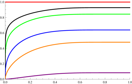
Figure 4: Plot of the observables ${\cal O}_{r,s}$, as a function of $t$, for the minimal model ${\cal M}(4,7)$. Reading from top to bottom, we plot ${\cal O}_{1,1},{1\over{\cal O}_{2,3}},{1\over{\cal O}_{1,2}},{\cal O}_{1,3},{\cal O}_{2,2},{\cal O}_{1,4}$ corresponding to $|\Delta_{r,s}^{4,7}|=0,{5\over 112},{1\over 14},{1\over 7},{27\over 112},{9\over 14}$ in increasing order with critical exponents $\beta_{r,s}={7\over 6}\,\Delta_{r,s}^{4,7}$. As expected for order parameters, these observables are nonegative, vanish at criticality and are increasing functions of $t$.

In this way, we have constructed observables with associated critical exponents for all conformal weights satisfying

$$\Delta_{r,s}^{m,m^{\prime}}<\Delta_{r_{0},s_{0}}^{m,m^{\prime}}+\frac{2(m^{\prime}-m)}{m^{\prime}}={1+(m^{\prime}-m)(9m-m^{\prime})\over 4mm^{\prime}}$$ (3.23)

These occur for $(r,s)$ in the Kac table satisfying $(m^{\prime}r-ms)^{2}<1+8m(m^{\prime}-m)$. In fact, we have constructed one such observable for each position $(r,s)$ in the Kac table but the conformal weights not satisfying (3.23) are masked because the correction terms are of lower order in the Taylor series expansion of (3.21). Some Kac tables showing the relevant exponents are shown in Table 2.

Table 2: Kac tables of conformal weights $\Delta_{r,s}^{m,m^{\prime}}$ for the minimal models ${\cal M}(2,5)$, ${\cal M}(4,7)$, ${\cal M}(5,7)$ respectively. The boxes of the conformal dimensions $\Delta_{r,s}<{1+(m^{\prime}-m)(9m-m^{\prime})\over 4mm^{\prime}}$ that are accessible, using Corner Transfer Matrices to calculate off-critical observables, are shaded in pink and occur in the band where $(r,s)$ satisfy $(m^{\prime}r-ms)^{2}<1+8m(m^{\prime}-m)$.

3.3 One point functions of the logarithmic minimal models

In this section, we apply the logarithmic limit (1.10) to the OPFs and GOPs of the Forrester-Baxter models. This is straightforward in the low-temperature nome. From (3.14), we find the limiting OPFs

$$P_{r,s}^{\infty}(q)=\frac{q^{\frac{c}{24}-\Delta^{p,p^{\prime}}_{r,s}+\frac{(s-r)(s-r-1)}{4}}E(q^{\frac{s}{2}},q^{\frac{m^{\prime}}{2(p^{\prime}-p)}})(q)_{\infty}}{E(-q^{\frac{1}{2}},q^{2})E(q^{\frac{r}{2}},q^{\frac{p}{2(p^{\prime}-p)}})}\ \chi^{p,p^{\prime}}_{r,s}(q),\qquad r,s=1,2,3,\ldots$$ (3.24)

The difficulty is in implementing a conjugate modulus transformation to the critical nome $t$ which is necessary to obtain the critical exponents. The problem derives from the fact that there is no simple conjugate modulus transformation on the infinity of the quasi-rational Kac characters $\chi_{r,s}^{p,p^{\prime}}(q)$. Indeed, it is easily seen that all of the entries (3.15) of the ${\cal S}$ matrix have a common prefactor $\sqrt{8/mm^{\prime}}$ which vanishes in the logarithmic limit. As a consequence, the conjugate modulus form (3.16) of the OPFs and the GOPs (3.17) (which both involve infinite sums) are not well behaved in the logarithmic limit. Nevertheless, the logarithmic limit of the observables ${\cal O}_{r,s}$ (3.21) (in which the problematic prefactors cancel out in the ratio) are well defined and admit a Taylor expansion about $t=0$

$${\cal O}_{r,s}^{\infty}=\lim_{m,m^{\prime}\to\infty,\ {m\over m^{\prime}}\to{p\over p^{\prime}}}\frac{R_{r,s}}{R_{1,1}}\sim(t^{\frac{\pi}{\lambda}})^{\Delta_{r,s}^{p,p^{\prime}}}+(t^{\frac{\pi}{\lambda}})^{\Delta_{r_{0},s_{0}}^{p,p^{\prime}}}O(t^{2}),\qquad\lambda={(p^{\prime}-p)\pi\over p^{\prime}}$$ (3.25)

This is just the logarithmic limit of the Taylor expansion (3.21) for the Forrester-Baxter observables. The limits of these Taylor expansions were checked using Mathematica [21].

We conclude that the associated logarithmic critical exponents are

$${\cal O}_{r,s}^{\infty}\sim(t^{2})^{\beta_{r,s}},\qquad\beta_{r,s}=(2-\alpha)\Delta_{r,s}^{p,p^{\prime}}=\frac{(rp^{\prime}-sp)^{2}-(p^{\prime}-p)^{2}}{8p(p^{\prime}-p)}$$ (3.26)

where the free energy exponent of the off-critical logarithmic minimal models $2-\alpha={\pi\over 2\lambda}=\frac{p^{\prime}}{2(p^{\prime}-p)}$, corresponding to the $\varphi_{1,3}$ perturbation off-criticality, is obtained in Appendix A. In this way, we have constructed limiting observables with associated critical exponents for all conformal weights satisfying

$$\Delta_{r,s}^{p,p^{\prime}}<\Delta_{r_{0},s_{0}}^{p,p^{\prime}}+\frac{2(p^{\prime}-p)}{p^{\prime}}={(p^{\prime}-p)(9p-p^{\prime})\over 4pp^{\prime}}$$ (3.27)

These occur for $(r,s)$ in the infinitely extended Kac tables satisfying $(p^{\prime}r-ps)^{2}<8p(p^{\prime}-p)$. The Kac tables of critical dense polymers ${\cal LM}(1,2)$ and critical percolation ${\cal LM}(2,3)$ showing the relevant exponents are presented in Table 1.

4 Conclusion

The face weights of the Forrester-Baxter models (associated with the non-unitary minimal models) can be decomposed by incorporating internal degrees of freedom, in the form of loop segments or bonds, that are suitable to describe generalized percolation or cluster properties. In this paper, we have used Corner Transfer Matrices to argue that the logarithmic limit (1.10) of the non-unitary minimal models ${\cal M}(m,m^{\prime};t)$ provides the integrable $\varphi_{1,3}$ off-critical perturbation of the logarithmic minimal models ${\cal LM}(p,p^{\prime})$. Generalized models of polymers and percolation can thus be solved exactly off-criticality. To support this assertion we have shown that, in accordance with the Kyoto correspondence principle [8], the limiting one-dimensional configurational sums yield the finitized quasi-rational Kac characters of the logarithmic theories. In addition, we have identified off-critical observables (3.21) in the minimal models that, in the logarithmic limit, exhibit critical exponents associated with conformal weights $\Delta_{r,s}^{p,p^{\prime}}$ in the infinitely extended Kac table of the logarithmic theory for all Kac labels $(r,s)$ satisfying $(ps-p^{\prime}r)^{2}<8p(p^{\prime}-p)$. We emphasize again that, although we call these limiting models off-critical logarithmic minimal models, these off-critical models are not expected to exhibit the indecomposable structures associated with critical logarithmic CFTs.

We believe that the evidence supporting our assertion is strong even though it is in a sense indirect. Perhaps our results could be obtained more directly by considering the unrestricted SOS models [11] with generic crossing parameter $\lambda$. If $\lambda$ is taken to be a rational fraction of $\pi$, this lattice model truncates to an RSOS model. However, we expect that the same off-critical logarithmic minimal models can be obtained if the logarithmic limit to a crossing parameter which is a rational fraction of $\pi$ is taken (through irrational fractions of $\pi$) after the thermodynamic limit.

The prototypical example of the logarithmic minimal models is percolation ${\cal LM}(2,3;t)$. The traditional approach to percolation [4] is to take either the limit $n\to 0$ [22] of the $n$-vector models or the limit $Q\to 1$ [23] of the $Q$-state Potts models. The drawback of these approaches is that they require an analytic continuation to non-integer $n$ or $Q$. A benefit of the current approach is that the logarithmic limit is completely under control since it is taken through a sequence of well-defined integrable lattice models.

The universal amplitude ratio $f_{\text{sing}}/M^{2}$ for the $\varphi_{1,3}$ perturbation of the minimal models ${\cal M}(m,m^{\prime})$ has been obtained from field theory by Lukyanov and Zamolodchikov [24]. Here the mass $M$ is proportional to the inverse correlation length. Universal amplitude ratios [25], for either the $\varphi_{1,3}$, $\varphi_{2,1}$ or $\varphi_{1,2}$ perturbations of the minimal models, can also be obtained from the lattice following [26]. It is then possible to obtain the universal amplitude ratios for the $\varphi_{1,3}$ perturbation of logarithmic minimal models, such as percolation ${\cal LM}(2,3)$. This is properly achieved by taking the logarithmic limit ($m\to\infty,m^{\prime}\to\infty,m/m^{\prime}\to p/p^{\prime}$). Previously, this step would have been taken by formally replacing $(m,m^{\prime})$ with $(p,p^{\prime})$ without justification. Using the logarithmic limit gives the same results but avoids the problem that, for example in the case $(p,p^{\prime})=(2,3)$, the naive replacement ${\cal M}(2,3)$ corresponds to a trivial theory rather than the correct percolation theory ${\cal LM}(2,3)$.

Figure 5: A link state of the logarithmic minimal model ${\cal LM}(p,p^{\prime})$ in the $(r,s)=(1,1)$ vacuum sector and the corresponding Dyck path $\sigma=\{1,2,1,2,3,2,3,2,1\}$ of length $N=8$ on (one-sided) $A_{\infty}$ with the boundary conditions $(\sigma_{0},\sigma_{N})=(1,1)$. The height $\sigma_{j}$ of the path at position $j=0,1,\ldots,N$ is equal to 1 plus the number of loops segments directly above position $j$ in the link state. The total number of such link states or Dyck paths under this bijection for $N$ even is given by the Catalan numbers $C_{N}={N!\over(N/2)!(N/2+1)!}$.

This paper opens up several directions for future research. First, rather than work with CTMs, it would be informative to apply the logarithmic limit (1.10) to the double-row transfer matrices of the minimal models on a strip both at criticality and off-criticality. The $(r,s)$ integrable boundary conditions for the non-unitary minimal models have not been studied in depth. Nevertheless at criticality, in the vacuum $(r,s)=(1,1)$ sector in which the boundary heights alternate between 1 and 2 on the left and right boundary edges of the strip, it is easy to see that the logarithmic limit of the conformal partition function is

$$Z^{m,m^{\prime}}_{(1,1)|(1,1)}(q)=\mbox{ch}^{m,m^{\prime}}_{r,s}(q)\to\chi_{r,s}^{p,p^{\prime}}(q)=q^{-c/24+\Delta_{r,s}^{p,p^{\prime}}}{(1-q)\over(q)_{\infty}}=Z^{p,p^{\prime}}_{(1,1)|(1,1)}(q)$$ (4.1)

We observe that, for these boundary conditions, the finite-size double-row transfer matrices have the same dimension in the sense that there is a bijection between the unrestricted SOS or Dyck paths on (one-sided) $A_{\infty}$ and the link states of the critical logarithmic minimal models as shown in Figure 5. It is therefore natural to expect that the logarithmic limit maps the finitized minimal Virasoro characters (2.28) onto the finitized quasi-rational Kac characters (2.45). More explicitly, for the non-unitary minimal models with Yang-Baxter integrable $(r,s)$ boundary conditions, we expect

$$Z^{m,m^{\prime},(N)}_{(1,1)|(r,s)}(q)=\mbox{ch}^{(N)}_{r,s}(q)\to\chi^{(N)}_{r,s}(q)=Z^{p,p^{\prime},(N)}_{(1,1)|(r,s)}(q)$$ (4.2)

where the characters implicitly depend on $b=b(r)$ given by (2.8) and the dependence of these characters on $m,m^{\prime}$ and $p,p^{\prime}$ is suppressed.

Likewise, it would be of interest to study the logarithmic limit of the periodic row transfer matrices of the minimal models both at criticality and off-criticality. At criticality, this could shed some light on the conjectured torus modular invariant partition functions [27, 28] of the logarithmic minimal models. The study of the logarithmic limit of the transfer matrices of the non-unitary models also opens up the possibility to obtain functional equations in the form of $T$- and $Y$-systems [29]. In particular, the off-critical functional relations could give a means to derive massive Thermodynamic Bethe Ansatz [30] equations for the logarithmic minimal models. Lastly, it would be of interest to study the logarithmic limit of the $\varphi_{2,1}$ and $\varphi_{1,2}$ off-critical integrable perturbations of the minimal models. This would involve further study of the non-unitary dilute $A$ lattice models [31]. We hope to come back to some of these problems later.

Appendix A Logarithmic Limit of the Forrester-Baxter Free Energy

The inversion relation method [32] has been used [7] to find the bulk partition function per site $\kappa(u)$, or equivalently, the free energy $f(u)=-\log\kappa(u)$ of the Forrester-Baxter models. In the notation of this paper,

$$\log\kappa(u)=u(\lambda-u)/\epsilon+2\sum_{n=1}^{\infty}\frac{\cosh((2\lambda-\pi)\pi n/\epsilon)\sinh(n\pi u/\epsilon)\sinh((\lambda-u)\pi n/\epsilon)}{n\sinh(\pi^{2}n/\epsilon)\cosh(\lambda\pi n/\epsilon)}$$ (A.1)

Using the Poisson summation formula, it can be shown that when $m^{\prime}-m\neq 1$ and $m^{\prime}$ is odd,

$$\log\kappa(u)=c(u,\lambda)-4\sum_{n=1}^{\infty}\frac{t^{2n}}{n(1-t^{2n})}\frac{\sin(nu)\sin((\lambda-u)n)\cos(2\lambda n)}{\cos(\lambda n)}\\ -4\sum_{n=1}^{\infty}\frac{t^{(2n-1)\pi/\lambda}}{(2n-1)(1-t^{(2n-1)\pi/\lambda})}\ \sin\frac{(2n-1)\pi u}{\lambda}\cot\frac{(2n-1)\pi^{2}}{2\lambda}$$ (A.2)

where $c(u,\lambda)$ is independent of the thermal deviation $t=e^{-\epsilon}$. This also gives the correct leading-order singularity and amplitude when $m^{\prime}-m\neq 1$ and $m^{\prime}$ is even, but the higher order terms in equation (A.2) are modified. At the isotropic point $u=\frac{\lambda}{2}$, the singular part $f_{\text{sing}}(u)$ of the free energy is

$$f_{\text{sing}}(\tfrac{\lambda}{2})\sim 4\,t^{\pi/\lambda}\cot\frac{\pi^{2}}{2\lambda}$$ (A.3)

with the critical exponent as given in [7].

This confirms that the deviation from criticality $t^{2}$ corresponds to the field $\varphi_{1,3}$ since, using the scaling relation on the associated critical exponent,

$$2-\alpha=\frac{m^{\prime}}{2(m^{\prime}-m)},\qquad\Delta_{t}=\frac{1-\alpha}{2-\alpha}=\frac{2m-m^{\prime}}{m^{\prime}}=\Delta_{1,3}^{m,m^{\prime}}$$ (A.4)

Since the amplitude and exponent depend on $m,m^{\prime}$ only through the ratio $\lambda$, these results (A.3) and (A.4) also apply in the logarithmic limit with $\lambda={(p^{\prime}-p)\pi\over p^{\prime}}$ and

$$\Delta_{t}=\frac{2p-p^{\prime}}{p^{\prime}}=\Delta_{1,3}^{p,p^{\prime}}$$ (A.5)

The amplitude of the leading singular term of the free energy

$$\mathcal{A}_{f}=4\cot\frac{\pi^{2}}{2\lambda}=-4\tan\frac{\pi m}{2(m^{\prime}-m)}$$ (A.6)

is used in the determination of the universal amplitude ratio $R_{\xi}^{+}$, or its equivalent in perturbed conformal field theory $f_{\text{sing}}/M^{2}$. The mass $M$ is proportional to the inverse correlation length, but it appears the correlation length $\xi$ of the Forrester-Baxter models has not yet been calculated. Nevertheless, (A.6) is consistent (at least in its dependence on $m$ and $m^{\prime}$) with the expression given by (14) of [24] for the $\varphi_{1,3}$ perturbation of $\mathcal{M}(m,m^{\prime})$

$${f_{\text{sing}}\over M^{2}}=-\frac{1}{4}\tan\frac{\pi m}{2(m^{\prime}-m)}$$ (A.7)

Appendix B Elliptic Functions

For convenience we summarize the definitions and properties of the elliptic functions used throughout this paper. The standard elliptic theta functions [9] are

$$\vartheta_{1}(u,t) =2t^{1/4}\sin u\prod_{n=1}^{\infty}(1-2t^{2n}\cos 2u+t^{4n})(1-t^{2n})$$ (B.1)

$$\vartheta_{4}(u,t) =\prod_{n=1}^{\infty}(1-2t^{2n-1}\cos 2u+t^{4n-2})(1-t^{2n})$$ (B.2)

with $\vartheta_{1}(u,t)=\vartheta_{2}(\tfrac{\pi}{2}-u,t)$ and $\vartheta_{3}(u,t)=\vartheta_{4}(\tfrac{\pi}{2}-u,t)$. We make use of the following identity (15.4.26) of [11] in writing the two forms of (2.3)

$$\vartheta_{4}(u)\vartheta_{4}(a\!-\!u)\vartheta_{1}(v)\vartheta_{1}(a\!-\!v)-\vartheta_{4}(v)\vartheta_{4}(a\!-\!v)\vartheta_{1}(u)\vartheta_{1}(a\!-\!u)=\vartheta_{4}(0)\vartheta_{4}(a)\vartheta_{1}(v\!-\!u)\vartheta_{1}(a\!-\!u\!-\!v)$$ (B.3)

The conjugate modulus transformations of the elliptic $\vartheta$-functions are

$$\vartheta_{1}(u,e^{-\epsilon}) =\sqrt{\frac{\pi}{\epsilon}}\,e^{-(u-\pi/2)^{2}/\epsilon}E(e^{-2\pi u/\epsilon},e^{-2\pi^{2}/\epsilon})$$ (B.4)

$$\vartheta_{4}(u,e^{-\epsilon}) =\sqrt{\frac{\pi}{\epsilon}}\,e^{-(u-\pi/2)^{2}/\epsilon}E(-e^{-2\pi u/\epsilon},e^{-2\pi^{2}/\epsilon})$$ (B.5)

where

$$E(x,q)=\sum_{k=-\infty}^{\infty}(-1)^{k}q^{k(k-1)/2}x^{k}=\prod_{n=1}^{\infty}(1-q^{n-1}x)(1-q^{n}x^{-1})(1-q^{n})$$ (B.6)

The elliptic $\vartheta$ functions also have infinite sum representations but we do not use them in this paper.

References

-
[1]
A.A. Belavin, A.M. Polyakov and A.B. Zamolodchikov,
Infinite conformal symmetry in two-dimensional quantum field theory,
Nucl. Phys. B241 (1984) 333–380;
Infinite conformal symmetry of critical fluctuations in two dimensions, J. Stat. Phys. 34 (1984) 763–774. -
[2]
J. Rasmussen,
Logarithmic limits of minimal models,
Nucl. Phys. B701 (2004) 516–528;
Jordan cells in logarithmic limits of conformal field theory, Int. J. Mod. Phys. A22 (2007) 67–82. - [3] P.A. Pearce, J. Rasmussen and J.-B. Zuber, Logarithmic minimal models, J. Stat. Mech. 0611 (2006) P017, arXiv:hep-th/0607232.
- [4] D. Stauffer and A. Aharony, Introduction to Percolation Theory, 2nd edition, London: Taylor and Francis, 1994.
- [5] H. Kesten, The critical probability of bond percolation on the square lattice equals 1/2, Commun. Math. Phys. 74 (1980) 41–59.
- [6] G.E. Andrews, R.J. Baxter and P.J. Forrester, Eight-vertex SOS model and generalised Rogers-Ramanujan-type identities, J. Stat. Phys. 35 (1984) 193–266.
- [7] P.J. Forrester and R.J. Baxter, Further exact solutions of the eight-vertex SOS model and generalizations of the Rogers-Ramanujan identities, J. Stat. Phys. 38 (1985) 435-472.
-
[8]
M. Jimbo, T. Miwa and M. Okado,
Solvable lattice models with broken symmetry and Hecke’s indefinite modular forms
Nucl. Phys. B275 (1986) 517–545;
E. Date, M. Jimbo, T. Miwa and M. Okado, Fusion of the eight vertex SOS model, Lett. Math. Phys. 12 (1986) 209–215; Automorphic properties of local height probabilities for integrable solid-on-solid models, Phys. Rev. B35 (1987) 2105–2107;
E. Date, M. Jimbo, A. Kuniba, T. Miwa and M. Okado, Exactly solvable SOS models: local height probabilities and theta function identities Nucl. Phys. B290 (1987) 231–273. - [9] I. S. Gradshteyn and I. M. Ryzhik, Tables of Integrals, Series and Products, New York; Sydney: Academic Press, 1980.
- [10] V.F.R. Jones, Planar algebras I (1999) math.QA/9909027.
- [11] R.J. Baxter, Exactly Solved Models in Statistical Mechanics, London: Academic Press, 1982.
-
[12]
A.L. Owczarek and R.J. Baxter,
A class of interaction-round-a-face models and its equivalence with an ice-type model,
J. Stat. Phys. 49 (1987) 1093–1115;
P.A. Pearce, Temperley-Lieb operators and critical -- lattice models, Int. J. Mod. Phys. B4 (1990) 715–734. - [13] H.N.V. Temperley and E.H. Lieb, Relations between the ‘percolation’ and ‘colouring’ problem and other graph-theoretical problems associated with regular planar lattices: some exact results for the ‘percolation’ problem, Proc. R. Soc. Lon. A322 (1971) 251–280.
- [14] V.F.R. Jones, Index for subfactors, Inventiones Math. 72 (1983) 1–25.
- [15] O. Foda and T.A. Welsh, On the combinatorics of Forrester-Baxter models, Physical Combinatorics (Kyoto, 1999), Progress in Mathematics 191 (2000) 49–103, Birkhauser, Boston, MA.
- [16] E. Melzer, Massive-conformal dictionary, Int. J. Mod Phys. A9 (1994) 5753–5768.
- [17] T. Trott, Summer Vacation Research Scholarship Project, University of Melbourne (2012), unpublished.
-
[18]
H. Riggs,
Solvable lattice models with minimal and nonunitary critical behaviour in two dimensions,
Nucl. Phys. B326 (1989) 673–688;
T. Nakanishi, Non-unitary minimal models and RSOS models, Nucl. Phys. B334 (1990) 745–766;
C. Itzykson, H. Saleur and J.-B. Zuber, Conformal invariance of nonunitary 2d-models, Europhys. Lett. 2 (1986) 91–96.
M. Lashkevich, Notes on scaling limits in SOS models, local operators and form factors, arXiv:hep-th/0510058 (2005). - [19] P. Di Francesco, P. Mathieu and D. Sénéchal, Conformal Field Theory, New York: Springer, 1997.
- [20] D.A. Huse, Exact exponents for infinitely many new multicritical points, Phys. Rev. B30 (1984) 3908–3915.
- [21] Mathematica 8, Wolfram Research, Inc., Champaign IL (2010).
- [22] P.G. de Gennes, Scaling Concepts in Polymer Physics, Ithaca, NY: Cornell University, 1979.
-
[23]
P.W. Kasteleyn and C.M. Fortuin,
Phase transitions in lattice systems with random local impurities,
J. Phys. Soc. Japan 26 Supp (1969) 11–14;
G. Delfino and J.L. Cardy, Universal amplitude ratios in the two-dimensional -state Potts model and percolation from quantum field theory, Nucl.Phys. B519 (1998) 551-578;
G. Delfino, J. Viti and J.L. Cardy Universal amplitude ratios of two-dimensional percolation from field theory, J. Phys. A: Math. Theor. 43 (2010) 152001 (7pp). - [24] S. Lukyanov and A. Zamolodchikov, Exact expectation values of local fields in quantum sine-Gordon model, Nucl.Phys. B493 (1997) 571–587.
-
[25]
G. Delfino,
Field theory of Ising percolating clusters,
Nucl. Phys. B818 (2009) 196–211;
G. Delfino and J. Viti, Universal properties of Ising clusters and droplets near criticality, Nucl. Phys. B840 (2010) 513–533. -
[26]
K.A. Seaton,
An exact universal amplitude ratio for percolation,
J. Phys. A: Math. Gen. 34 (2001) L759-L762;
A universal amplitude ratio for the Potts model from a solvable lattice model, J. Stat. Phys. 107 (2002) 1255-1265. - [27] M.R. Gaberdiel, I. Runkel and S. Wood, A modular invariant bulk theory for the triplet model, J. Phys. A44 (2011) 015204.
- [28] P.A. Pearce and J. Rasmussen, Coset graphs in bulk and boundary logarithmic minimal models, Nucl. Phys. B846 (2011) 616–649.
-
[29]
A. Klümper and P.A. Pearce,
Conformal weights of RSOS lattice models and their fusion hierarchies,
Physica A183 (1992) 304–350;
A. Kuniba, T. Nakanishi and J. Suzuki, Functional relations in solvable lattice models: I Functional relations and representation theory, Int. J. Mod. Phys. A9 (1994) 5215–5266;
-systems and -systems in integrable systems, J. Phys. A44 (2011) 103001. -
[30]
A.B. Zamolodchikov,
On the reflectionless Bethe ansatz equations for reflectionless scattering theories,
Phys. Lett. B253 (1991) 391–394;
Thermodynamic Bethe ansatz for RSOS scattering theories, Nucl. Phys. B358 (1991) 497–523;
TBA equations for integrable perturbed coset models, Nucl. Phys. B366 (1991) 122–132. -
[31]
S.O. Warnaar, B. Nienhuis and K.A. Seaton,
New construction of solvable lattice models including an Ising model in a field,
Phys. Rev. Lett. 69 (1992) 710–712.
S.O. Warnaar, P.A. Pearce, K.A. Seaton and B. Nienhuis, Order parameters of the dilute models, J. Stat. Phys. 74 (1994) 469–531. - [32] R. J. Baxter, The inversion relation method for some two-dimensional exactly solved models in lattice statistics, J. Stat. Phys. 28 (1982) 1–41.