Non-asymptotic fractional order differentiators via an algebraic parametric method

Abstract

Recently, Mboup, Join and Fliess [27, 28] introduced non-asymptotic integer order differentiators by using an algebraic parametric estimation method [7, 8]. In this paper, in order to obtain non-asymptotic fractional order differentiators we apply this algebraic parametric method to truncated expansions of fractional Taylor series based on the Jumarie’s modified Riemann-Liouville derivative [14]. Exact and simple formulae for these differentiators are given where a sliding integration window of a noisy signal involving Jacobi polynomials is used without complex mathematical deduction. The efficiency and the stability with respect to corrupting noises of the proposed fractional order differentiators are shown in numerical simulations.

I INTRODUCTION

Fractional models arise in many practical situations ([3, 37] for example). Such fractional order systems may also be used for control purposes: CRONE control is known to have good robustness properties (see [33, 34, 35, 37]). In order to implement such controller one needs to have a good digital fractional order differentiator from noisy signals, which is the scope of this paper.

The fractional derivative has a long history and has often appeared in science, engineering and finance (see, e.g., [32, 36, 12, 4]). Different from classical integer order derivative, there are several kinds of definitions for the fractional derivative which are generally not equivalent with each other [36, 17]. Among these definitions, the Riemann-Liouville derivative and the Caputo derivative are often used [36]. Recently, a new modified Riemann-Liouville derivative is proposed by Jumarie [14]. This new definition of fractional derivative has two main advantages: firstly comparing with the Caputo derivative, the function to be differentiated is not necessarily differentiable, secondly different from the Riemann-Liouville derivative the Jumarie’s modified Riemann-Liouville derivative of a constant is defined to zero. Moreover, a fractional Taylor series expansion [13] was invented by using this new definition. Thanks to these merits, the Jumarie’s modified Riemann-Liouville derivative was successfully applied (see, e.g., [15, 16, 43]). The fractional order differentiator is concerned with estimating the fractional order derivatives of an unknown signal from its noisy observed data. Because of its importance, various methods have been developed during the last years ([2, 25] for example). However, the obtained fractional order differentiators were usually based on the Riemann-Liouville derivative and the Caputo derivative. To our knowledge, there is no one based on the Jumarie’s modified Riemann-Liouville derivative.

Recent algebraic parametric estimation method for linear systems [7, 8, 44] has been extended to various problems in signal processing (see, e.g., [9, 10, 26, 30, 31, 42, 41, 19, 18]). Let us emphasize that this method is algebraic and non-asymptotic, which provides explicit formulae and finite-time estimates. Moreover, it exhibits good robustness properties with respect to corrupting noises, without the need of knowing their statistical properties (see [5, 6] for more theoretical details). The robustness properties have already been confirmed by numerous computer simulations and several laboratory experiments. Very recently, this method was used to solve the ill-posed numerical differentiation problem in [27, 28]. The main idea is to apply a differentiator called integral-annihilator to a truncated Taylor series expansion which is a local approximation of the signal to be differentiated. Stable non-asymptotic differentiators of integer order were exactly given by the integrals of noisy signals involving the Jacobi orthogonal polynomials. The associated estimation errors were studied in [20, 22, 23]. An extension of these differentiators for multivariate numerical differentiation were proposed in [38, 39, 40]. However, this method has not been used to estimate fractional order derivatives.

The aim of this paper is to introduce non-asymptotic fractional order differentiators for the Jumarie’s modified Riemann-Liouville derivative by using the algebraic parametric method. In Section II, we recall how to apply the algebraic parametric method to obtain an integer order differentiator from a truncated Taylor series expansion. Section III begins with the definition of the Jumarie’s modified Riemann-Liouville derivative. Then, two fractional order differentiators are obtained by applying integral-annihilators to truncated fractional Taylor series expansions with different truncated orders. Moreover, it is shown that the differentiator obtained from higher order truncated expansion can be expressed as an affine combination of the ones obtained from lower order truncated expansion. Numerical tests are given in Section IV. They help us to show the efficiency and the stability of the proposed fractional order differentiators. Finally, we give some conclusions and perspectives for our future work in Section V.

II METHODOLOGY

Let $y=x+\varpi$ be a noisy signal observed in an open interval $I\subset\mathbb{R}$, where $x\in\mathcal{C}^{n}(I)$ with $n\in\mathbb{N}$ and the noise $\varpi$ is bounded and integrable. In this section, we are going to recall how to use an algebraic parametric method to estimate the integer order derivatives of $x$ [27, 28].

For any $t_{0}\in I$, we introduce the set $D_{t_{0}}:=\{t\in\mathbb{R}_{+};\,t_{0}+t\in I\}$. By using the famous Taylor’s formula formulated by Hardy ([11] p. 293), we obtain that $\forall\,t_{0}\in I,\ t\in D_{t_{0}},$

$$x(t_{0}+t) =\sum_{j=0}^{n}\frac{t^{j}}{j!}x^{(j)}(t_{0})+\mathcal{O}(t^{n}),\ \text{ as }t\rightarrow 0.$$ (1)

In a similar way to classical numerical differentiation methods, the algebraic parametric method uses the $n^{th}$ order derivative of a polynomial to estimate the one of $x$. Here, we consider the following truncated Taylor series expansion of $x$ on $\mathbb{R}_{+}$

$$\forall\,t\in\mathbb{R}_{+},\ x_{n}(t_{0}+t):=\sum_{j=0}^{n}\frac{t^{j}}{j!}x^{(j)}(t_{0}).$$ (2)

Different from the other methods, the $n^{th}$ order derivative of the approximation polynomial $x_{n}$ is calculated by applying algebraic manipulations to $x_{n}$ in the operational domain. Precisely, we apply a differential operator with the following form [22]

$$\Pi^{n}_{k,\mu}=\frac{1}{s^{n+1+\mu}}\cdot\frac{d^{n+k}}{ds^{n+k}}\cdot{s^{n}},$$ (3)

where $-1<\mu\in\mathbb{R}$ and $k\in\mathbb{N}$. This differential operator was introduced in [28] with $\mu\in\mathbb{N}$.

Let us mention that the operation $\frac{d^{n+k}}{ds^{n+k}}\cdot{s^{n}}$ is used to annihilate all the terms containing $x^{(j)}(t_{0})$ with $0\leq j\leq n-1$ in $x_{n}$ in the operational domain, and the rational term $\frac{1}{s^{n+1+\mu}}$ permits to obtain a Riemann-Liouville integral [24] expression for $x^{(n)}(t_{0})$ in the time domain (see the next section for more details). Thus, the differential operator $\Pi^{n}_{k,\mu}$ is called integral-annihilator for $x^{(n)}(t_{0})$ via $x_{n}$ [28]. Finally, if we replace $x_{n}$ by $y$ in the obtained integral expression, then we can obtain the following estimator for $x^{(n)}(t_{0})$ (see [22] and [28] for more details)

$$\begin{split}&\forall\,t_{0}\in I,\ \tilde{y}^{(n)}_{{t_{0}}}(k,\mu,T):=\\ &\quad\ \ \frac{n!}{T^{n}}\gamma_{n,k,\mu}\int_{0}^{1}w_{\mu,k}(\tau)P^{(\mu,k)}_{n}(\tau)\,y(t_{0}+T\tau)\,d\tau,\end{split}$$ (4)

where $T\in D_{t_{0}}$, $\gamma_{n,k,\mu}=\frac{1}{\mathrm{B}(n+k+1,n+\mu+1)}$, $\mathrm{B}(\cdot,\cdot)$ is the classical beta function ([1], p. 258), $P^{(\mu,k)}_{n}$ is the $n^{th}$ order Jacobi polynomial ([1] p. 775) defined on $[0,1]$ as follows

$${P}_{n}^{(\mu,k)}(\tau)=\displaystyle\sum_{j=0}^{n}\binom{n+\mu}{j}\binom{n+k}{n-j}\left({\tau-1}\right)^{n-j}\left(\tau\right)^{j},$$ (5)

and $w_{\mu,k}(\tau)=(1-\tau)^{\mu}\tau^{k}$ is the associated weight function. Hence, this differentiator depends on three parameters $k$, $\mu$, $T$. Moreover, it is a non-asymptotic pointwise differentiator using the sliding integration window $[t_{0},t_{0}+T]$. Since $\tilde{y}^{(n)}_{{t_{0}}}(k,\mu,T)$ is obtained by taking an $n^{th}$ order polynomial where $n$ is the order of the derivative estimated, we call it minimal Jacobi differentiator.

III NON-ASYMPTOTIC FRACTIONAL ORDER DIFFERENTIATOR

In this section, we are going to propose two fractional order differentiators by applying the algebraic parametric method to different truncated expansions of the fractional Taylor series based on the Jumarie’s modified Riemann-Liouville derivative [14, 13].

III-A The Jumarie’s modified Riemann-Liouville derivative

Let $f$ be a continuous function defined on $\mathbb{R}$, then the Jumarie’s modified Riemann-Liouville derivative of $f$ is defined as follows [14]

$$f^{(\alpha)}(t):=\frac{1}{\Gamma(l-\alpha)}\frac{d^{l}}{dt^{l}}\int_{0}^{t}\frac{f(\tau)-f(0)}{\left(t-\tau\right)^{\alpha+1-l}}\,d\tau,$$ (6)

where $0\leq l-1\leq\alpha<l$ with $l\in\mathbb{N}^{\ast}$. This fractional order derivative is in fact defined through the fractional difference [14]

$$f^{(\alpha)}(t):=\lim_{h\rightarrow 0}\frac{\Delta^{\alpha}\left[f(t)-f(0)\right]}{h^{\alpha}},$$ (7)

where $h>0$, $FW\,f(t)=f(t+h)$ and

$$\begin{split}\Delta^{\alpha}f(t)&=\left(FW-1\right)^{\alpha}f(t)\\ &=\sum^{\infty}_{i=0}(-1)^{i}\binom{\alpha}{i}f\left[t+(\alpha-i)h\right].\end{split}$$ (8)

Let us recall that the Riemann-Liouville derivative is defined as follows ([36] p. 62)

$${}_{0}{D}_{t}^{\alpha}f(t):=\frac{1}{\Gamma(l-\alpha)}\frac{d^{l}}{dt^{l}}\int_{0}^{t}\frac{f(\tau)}{\left(t-\tau\right)^{\alpha+1-l}}\,d\tau,$$ (9)

where $0\leq l-1\leq\alpha<l$ with $l\in\mathbb{N}^{\ast}$. If we take $f(t)=t^{n}$ with $n\in\mathbb{N}$ and $t\in\mathbb{R}_{+}^{\ast}$, then we obtain (see [36] p. 72)

$${}_{0}{D}_{t}^{\alpha}t^{n}=\frac{\Gamma(n+1)}{\Gamma(n+1-\alpha)}\,t^{n-\alpha},\ \text{ with }\alpha\in\mathbb{R}_{+}.$$ (10)

Consequently, the Jumarie’s modified Riemann-Liouville derivative can be expressed as follows

$$\forall\,t\in\mathbb{R}_{+}^{\ast},\ f^{(\alpha)}(t)={}_{0}{D}_{t}^{\alpha}f(t)-\frac{t^{-\alpha}}{\Gamma(1-\alpha)}\,f(0).$$ (11)

One of some useful properties of the Jumarie’s modified Riemann-Liouville derivative is the fractional Leibniz derivative rule [14]

$$\left(f\,g\right)^{(\alpha)}=f^{(\alpha)}g+g^{(\alpha)}f.$$ (12)

Moreover, since $x\in\mathcal{C}^{n}(I)$, a generalized Taylor series expansion based on the Jumarie’s modified Riemann-Liouville derivative of $x$ is given as follows [14, 13]: $\forall\,t_{0}\in I$, $t\in D_{t_{0}}$,

$$x(t_{0}+t)=\sum_{j=0}^{n}\frac{t^{j}}{j!}x^{(j)}(t_{0})+\sum_{j=1}^{+\infty}\frac{t^{j\gamma+n}}{\Gamma(j\gamma+n+1)}x^{(j\gamma+n)}(t_{0}),$$ (13)

where $\gamma=\alpha-n$ with $n<\alpha\leq n+1$.

Let us remark that the fractional order derivative $x^{(j\gamma+n)}$ in (13) should be understood as $(x^{(n)})^{(j\gamma)}$ which is different from $(x^{(j\gamma)})^{(n)}$ [14].

III-B Minimal Jacobi fractional differentiator

By using (13), we take the following truncated fractional Taylor series expansion of $x$ on $\mathbb{R}^{+}$: $\forall\,t_{0}\in I$, $t\in\mathbb{R}^{+}$,

$$x_{\alpha}(t_{0}+t):=\sum_{j=0}^{n}\frac{t^{j}}{j!}x^{(j)}(t_{0})+\frac{t^{\alpha}}{\Gamma(\alpha+1)}x^{(\alpha)}(t_{0}).$$ (14)

Then, by using the algebraic parametric method we can give the following proposition.

Proposition 1

Let $y=x+\varpi$ be a noisy signal observed on an open interval $I\subset\mathbb{R}$, where $x\in\mathcal{C}^{n}(I)$ with $n<\alpha\leq n+1$, $n\in\mathbb{N}$, and $\varpi$ be a bounded and integrable noise. Then an estimator for the $\alpha^{th}$ order derivative value $x^{(\alpha)}(t_{0})$ is given by: $\forall\,t_{0}\in I$,

$$\begin{split}&\tilde{y}^{(\alpha)}_{{t_{0}}}(k,\mu,T):=\\ &\frac{(n+1)!}{T^{\alpha}}\gamma_{n,k,\mu,\alpha}\int_{0}^{1}w_{\mu,k}(\tau)P^{(\mu,k)}_{n+1}(\tau)\,y(t_{0}+T\tau)\,d\tau,\end{split}$$ (15)

where $T\in D_{t_{0}}$, $\gamma_{n,k,\mu,\alpha}=\frac{\Gamma(\alpha-n)}{\mathrm{B}(\alpha+1+k,n+\mu+2)}$, and $P^{(\mu,k)}_{n+1}$ is the Jacobi polynomial defined by (5) with $k\in\mathbb{N}$ and $-1<\mu\in\mathbb{R}$.

Proof. By applying the Laplace transform to $(\ref{Eq_Taylor_series_fractional_truncated})$, we get

$$\hat{x}_{\alpha}(s)=\sum_{j=0}^{n}s^{-(j+1)}x^{(j)}(t_{0})+s^{-(\alpha+1)}x^{(\alpha)}(t_{0}),$$ (16)

where $\hat{x}_{\alpha}(s)$ is the Laplace transform of $x_{\alpha}(t_{0}+t)$, and $s$ is the Laplace variable.

We are going to apply some algebraic manipulations to (16). Firstly, we apply the operation $\frac{d^{n+1+k}}{ds^{n+1+k}}\cdot s^{n+1}$ to (16) so as to annihilate the terms containing $x^{(j)}(t_{0})$ with $0\leq j\leq n$ in $\hat{x}_{\alpha}$. Thus, we get

$$\begin{split}&\frac{d^{n+1+k}}{ds^{n+1+k}}s^{n+1}\left(\sum_{j=0}^{n}s^{-(j+1)}x^{(j)}(t_{0})+s^{-(\alpha+1)}x^{(\alpha)}(t_{0})\right)\\ =&(-1)^{n+1+k}\frac{\Gamma(\alpha+1+k)}{\Gamma(\alpha-n)}\frac{1}{s^{\alpha+k+1}}x^{(\alpha)}(t_{0}).\end{split}$$

Secondly, if we apply the Leibniz derivative rule to $\frac{d^{n+1+k}}{ds^{n+1+k}}s^{n+1}\hat{x}_{\alpha}(s)$, then the highest order of $s$ in the obtained sum is $n+1$. Hence, we choose the rational term $\frac{1}{s^{n+2+\mu}}$ with $\mu>-1$ such that $\frac{1}{s^{n+2+\mu}}\cdot s^{n+1}=\frac{1}{s^{1+\mu}}$ with $\mu+1>0$. This permits to obtain a Riemann-Liouville integral [24] expression of $x_{\alpha}$ in the time domain. Consequently, we construct an integral-annihilator for $x^{(\alpha)}(t_{0})$ via $x_{\alpha}$ which corresponds to the operator $\Pi^{n+1}_{k,\mu}$ defined by (3).

Consequently, by applying the inverse Laplace transform and the classical rules of operational calculus, we get

$$\begin{split}&\mathcal{L}^{-1}\left\{\Pi^{n+1}_{k,\mu}\left(\sum_{j=0}^{n}s^{-(j+1)}x^{(j)}(t_{0})+s^{-(\alpha+1)}x^{(\alpha)}(t_{0})\right)\right\}(T)=\\ &\quad\quad\quad(-1)^{n+1+k}\frac{\Gamma(\alpha+1+k)}{\Gamma(\alpha-n)}\frac{T^{n+\alpha+2+k+\mu}}{\Gamma(n+\alpha+k+\mu+3)}x^{(\alpha)}(t_{0}),\\ &\mathcal{L}^{-1}\left\{\Pi^{n+1}_{k,\mu}\hat{x}_{\alpha}(s)\right\}(T)=\\ &\quad\frac{(-1)^{n+1+k}}{\Gamma(n+\mu+2)}\int_{0}^{T}(T-\tau)^{n+\mu+1}\tau^{n+k+1}x^{(n+1)}_{\alpha}(t_{0}+\tau)d\tau.\end{split}$$ (17)

By applying a change of variable $\tau\rightarrow T\tau$ and $n+1$ times integrations by parts, we get

$$\begin{split}&\frac{(-1)^{(n+1)}T^{\alpha}}{\gamma_{n,k,\mu,\alpha}}\,x^{(\alpha)}(t_{0})=\\ &\int_{0}^{1}\frac{d^{n+1}}{d\tau^{n+1}}\left\{(1-\tau)^{n+\mu+1}\tau^{n+k+1}\right\}x_{\alpha}(t_{0}+T\tau)\,d\tau.\end{split}$$ (18)

Finally, this proof can be completed by substituting $x_{\alpha}$ in (LABEL:Eq_estimator_fractional0) by $y$ and applying the Rodrigues formula ([1] p. 785) to the right side of (LABEL:Eq_estimator_fractional0). $\Box$

Since the differentiator $\tilde{y}^{(\alpha)}_{{t_{0}}}(k,\mu,T)$ involves a Jacobi polynomial, and it is obtained by taking the minimal order ($j=1$) truncated fractional Taylor series expansion in (13), we call it minimal Jacobi fractional differentiator. The corresponding truncated error part comes from the truncated term $\displaystyle\sum_{j=2}^{+\infty}\frac{t^{(j\gamma+n)}}{\Gamma(j\gamma+n+1)}x^{(j\gamma+n)}(t_{0})$. If we take $\alpha=n+1$ in (LABEL:Eq_estimator_fractional), then it is easy to obtain that

$$\tilde{y}^{(\alpha)}_{{t_{0}}}(k,\mu,T)=\tilde{y}^{(n+1)}_{{t_{0}}}(k,\mu,T),$$ (19)

where $\tilde{y}^{(n+1)}_{{t_{0}}}(k,\mu,T)$ is the minimal Jacobi differentiator for $x^{(n+1)}(t_{0})$ given in (LABEL:Eq_minimal_estimator). Moreover, in a similar way to the minimal Jacobi differentiator method, the minimal Jacobi fractional differentiator $\tilde{y}^{(\alpha)}_{{t_{0}}}(k,\mu,T)$ can also be obtained by using the classical orthogonal properties of the Jacobi polynomials to (14) (see [21] for more details). Consequently, as done in [22], the parameter $k$ which is defined on $\mathbb{N}$ can also be extended to $]-1,+\infty[$.

Finally, let us recall that the affine Jacobi differentiator being an affine combination of the minimal Jacobi differentiators was introduced in [27, 28] by applying the algebraic parametric method to a higher order truncated Taylor series expansion than (2). Hence, the convergence rate for the Jacobi differentiator was improved. Similarly to the integer derivative case, we are going to introduce an Affine Jacobi fractional differentiator in the next subsection.

III-C Affine Jacobi fractional differentiator

In this subsection, we take a new truncated fractional Taylor series expansion in (13) up to $j=2$: $\forall\,t_{0}\in I$, $t\in\mathbb{R}^{+}$,

$$\begin{split}&x_{2\alpha-n}(t_{0}+t)=\sum_{j=0}^{n}\frac{t^{j}}{j!}x^{(j)}(t_{0})\\ &+\frac{t^{\alpha}}{\Gamma(\alpha+1)}x^{(\alpha)}(t_{0})+\frac{t^{2\alpha-n}}{\Gamma(2\alpha-n+1)}x^{(2\alpha-n)}(t_{0}).\end{split}$$ (20)

In order to obtain an estimator for $x^{(\alpha)}(t_{0})$ from this truncated expansion, we introduce the following differential operator

$$\Pi^{n+1}_{k,\mu,\alpha}=\frac{1}{s^{2\alpha+k+\mu+3}}\cdot\frac{d}{ds}\cdot s^{2\alpha-n+1+k}\cdot\frac{d^{n+k+1}}{ds^{n+k+1}}\cdot s^{n+1},$$ (21)

where $-1<\mu\in\mathbb{R}$, $k\in\mathbb{N}$ and $n<\alpha\leq n+1$ with $n\in\mathbb{N}$. Then, we give the following proposition.

Proposition 2

The differential operator $\Pi^{n+1}_{k,\mu,\alpha}$ defined in (21) is an integral-annihilator for $x^{(\alpha)}(t_{0})$ via $x_{2\alpha-n}$ defined in (20).

Proof. Applying the Laplace transform to $(\ref{Eq_Taylor_series_fractional_truncated2})$, we get

$$\begin{split}&\hat{x}_{2\alpha-n}(s)=\sum_{j=0}^{n}s^{-(j+1)}x^{(j)}(t_{0})\\ &\quad\quad+s^{-(\alpha+1)}x^{(\alpha)}(t_{0})+s^{-(2\alpha-n+1)}x^{(2\alpha-n)}(t_{0}),\end{split}$$ (22)

where $\hat{x}_{2\alpha-n}(s)$ is the Laplace transform of $x_{2\alpha-n}(t_{0}+t)$.

We are going to apply $\Pi^{n+1}_{k,\mu,\alpha}$ to (22). Firstly, we apply the operation $\frac{d^{n+1+k}}{ds^{n+1+k}}\cdot s^{n+1}$ to (22) so as to annihilate the terms containing $x^{(j)}(t_{0})$ with $0\leq j\leq n$ in $\hat{x}_{2\alpha-n}$. Thus, we obtain

$$\begin{split}&\frac{d^{n+1+k}}{ds^{n+1+k}}s^{n+1}\left(\hat{x}_{2\alpha-n}(s)\right)=\\ &\quad(-1)^{n+1+k}\frac{\Gamma(\alpha+1+k)}{\Gamma(\alpha-n)}\frac{1}{s^{\alpha+k+1}}x^{(\alpha)}(t_{0})\\ +&(-1)^{n+1+k}\frac{\Gamma(2\alpha-n+1+k)}{\Gamma(2\alpha-2n)}\frac{x^{(2\alpha-n)}(t_{0})}{s^{2\alpha-n+k+1}}.\end{split}$$ (23)

Secondly, we apply the operator $\frac{d}{ds}\cdot s^{2\alpha-n+1+k}$ to (LABEL:Eq_Taylor_series_fractional_laplace3) so as to annihilate the term containing $x^{(2\alpha-n)}(t_{0})$ in $\hat{x}_{2\alpha-n}$. This yields

$$\begin{split}&\frac{d}{ds}s^{2\alpha-n+1+k}\frac{d^{n+1+k}}{ds^{n+1+k}}s^{n+1}\left(\hat{x}_{2\alpha-n}(s)\right)=\\ &\quad(-1)^{n+1+k}\frac{\Gamma(\alpha+1+k)}{\Gamma(\alpha-n)}(\alpha-n)s^{\alpha-n-1}x^{(\alpha)}(t_{0}).\end{split}$$ (24)

Thirdly, if we apply the Leibniz derivative rule to $\frac{d}{ds}s^{2\alpha-n+1+k}\frac{d^{n+1+k}}{ds^{n+1+k}}s^{n+1}\hat{x}_{2\alpha-n}(s)$, then the highest order of $s$ in the obtained sum is $2\alpha+n+k+2$. Hence, we apply the rational term $\frac{1}{s^{2\alpha+n+k+3+\mu}}$ with $\mu>-1$ such that $\frac{1}{s^{2\alpha+n+k+3+\mu}}\cdot s^{2\alpha+n+k+2}=\frac{1}{s^{1+\mu}}$ with $\mu+1>0$. This allows us to obtain a Riemann-Liouville integral expression of $x_{2\alpha-n}$ in the time domain. Consequently, $\Pi^{n+1}_{k,\mu,\alpha}$ is an integral-annihilator for $x^{(\alpha)}(t_{0})$ via $x_{2\alpha-n}$. Moreover, we have

$$\begin{split}&(-1)^{n+1+k}\,\mathcal{L}^{-1}\left\{\Pi^{n+1}_{k,\mu,\alpha}\hat{x}_{2\alpha-n}(s)\right\}(T)=\\ &\frac{\Gamma(\alpha+1+k)}{\Gamma(\alpha-n)}\frac{(\alpha-n)\,T^{n+\alpha+3+k+\mu}}{\Gamma(n+\alpha+k+\mu+4)}x^{(\alpha)}(t_{0}),\end{split}$$ (25)

where $T\in D_{t_{0}}$. $\Box$

Similarly to Proposition 1, by substituting $x_{2\alpha-n}$ by $y$ in the obtained Riemann-Liouville integral $\mathcal{L}^{-1}\left\{\Pi^{n+1}_{k,\mu,\alpha}\hat{x}_{2\alpha-n}\right\}(T)$, we obtain a new estimator for $x^{(\alpha)}(t_{0})$. We denote it by $\tilde{y}^{(\alpha)}_{{t_{0}}}(k,\mu,T,\alpha)$. Then, we get the following proposition.

Proposition 3

Let $y$ be a noisy signal defined as in Proposition 1, then we have the following affine relation

$$\begin{split}\tilde{y}^{(\alpha)}_{{t_{0}}}(k,\mu,T,\alpha)&=\lambda_{\alpha,k,n}\,\tilde{y}^{(\alpha)}_{{t_{0}}}(k,\mu+1,T)\\ &+(1-\lambda_{\alpha,k,n})\,\tilde{y}^{(\alpha)}_{{t_{0}}}(k+1,\mu,T),\end{split}$$ (26)

where $\lambda_{\alpha,k,n}=\frac{2\alpha-n+1+k}{\alpha-n}$. The differentiator $\tilde{y}^{(\alpha)}_{{t_{0}}}(k,\mu,T,\alpha)$ is thus called affine Jacobi fractional differentiator.

In order to prove the above proposition, we need the following lemma.

Lemma 1

Let $\hat{f}$ be the Laplace transform of an analytic function $f$ defined on $I$, $\Pi^{n+1}_{k,\mu,\alpha}$ and $\Pi^{n+1}_{k,\mu}$ be the integral-annihilators defined in (21) and (3) respectively, then we have

$$\begin{split}&\Pi^{n+1}_{k,\mu,\alpha}\hat{f}(s)=\\ &\quad\quad(2\alpha-n+1+k)\,\Pi^{n+1}_{k,\mu+1}\hat{f}(s)+\Pi^{n+1}_{k+1,\mu}\hat{f}(s).\end{split}$$ (27)

Proof. By applying the Leibniz derivative rule, we get

$$\Pi^{n+1}_{k,\mu,\alpha}\hat{f}(s)$$

$$= \frac{1}{s^{2\alpha+k+\mu+3}}\left((2\alpha-n+1+k)s^{2\alpha-n+k}\frac{d^{n+k+1}}{ds^{n+k+1}}s^{n+1}\hat{f}(s)\right)$$

$$+\frac{1}{s^{2\alpha+k+\mu+3}}\left(s^{2\alpha-n+k+1}\frac{d^{n+k+2}}{ds^{n+k+2}}s^{n+1}\hat{f}(s)\right)$$

$$= (2\alpha-n+1+k)\Pi^{n+1}_{k,\mu+1}\hat{f}(s)+\Pi^{n+1}_{k+1,\mu}\hat{f}(s).$$

$\Box$

Proof of Proposition 3. According to (LABEL:Eq_2), we obtain

$$\begin{split}&\mathcal{L}^{-1}\left\{\Pi^{n+1}_{k,\mu,\alpha}\hat{x}_{2\alpha-n}(s)\right\}(T)\\ =&\mathcal{L}^{-1}\left\{\Pi^{n+1}_{k,\mu,\alpha}\left(\sum_{j=0}^{n}s^{-(j+1)}x^{(j)}(t_{0})+s^{-(\alpha+1)}x^{(\alpha)}(t_{0})\right)\right\}(T)\\ =&\mathcal{L}^{-1}\left\{\Pi^{n+1}_{k,\mu,\alpha}\hat{x}_{\alpha}(s)\right\}(T)\\ =&(-1)^{n+1+k}\frac{\Gamma(\alpha+1+k)}{\Gamma(\alpha-n)}\frac{(\alpha-n)T^{n+\alpha+3+k+\mu}}{\Gamma(n+\alpha+k+\mu+4)}x^{(\alpha)}(t_{0}).\end{split}$$ (28)

By substituting $x_{\alpha}$ by $x$ in the Riemann-Liouville integrals $\mathcal{L}^{-1}\left\{\Pi^{n+1}_{k,\mu,\alpha}\hat{x}_{\alpha}(s)\right\}(T)$ and $\mathcal{L}^{-1}\left\{\Pi^{n+1}_{k,\mu}\hat{x}_{\alpha}(s)\right\}(T)$ given in (LABEL:Eq_3) and (17) respectively, we get

$$\begin{split}\tilde{x}^{(\alpha)}_{{t_{0}}}(k,\mu,T,\alpha):=&\frac{c_{n,k,\mu,\alpha,T}}{\alpha-n}\mathcal{L}^{-1}\left\{\Pi^{n+1}_{k,\mu,\alpha}\hat{x}(s)\right\}(T)\\ \tilde{x}^{(\alpha)}_{{t_{0}}}(k,\mu+1,T):=&c_{n,k,\mu,\alpha,T}\mathcal{L}^{-1}\left\{\Pi^{n+1}_{k,\mu+1}\hat{x}(s)\right\}(T)\\ \tilde{x}^{(\alpha)}_{{t_{0}}}(k+1,\mu,T):=&-\frac{c_{n,k,\mu,\alpha,T}}{\alpha+1+k}\mathcal{L}^{-1}\left\{\Pi^{n+1}_{k+1,\mu}\hat{x}(s)\right\}(T),\end{split}$$ (29)

where $c_{n,k,\mu,\alpha,T}=(-1)^{n+1+k}\frac{\Gamma(\alpha-n)}{\Gamma(\alpha+1+k)}\frac{\Gamma(n+\alpha+k+\mu+4)}{T^{n+\alpha+3+k+\mu}}$. Hence, by using Lemma 1 we obtain

$$\begin{split}\tilde{x}^{(\alpha)}_{{t_{0}}}(k,\mu,T,\alpha)&=\lambda_{\alpha,k,n}\,\tilde{x}^{(\alpha)}_{{t_{0}}}(k,\mu+1,T)\\ &+(1-\lambda_{\alpha,k,n})\,\tilde{x}^{(\alpha)}_{{t_{0}}}(k+1,\mu,T).\end{split}$$ (30)

Finally, this proof can be completed by substituting $x$ by $y$ in $\tilde{x}^{(\alpha)}_{{t_{0}}}(k,\mu,T,\alpha)$, $\tilde{x}^{(\alpha)}_{{t_{0}}}(k+1,\mu,T,\alpha)$ and $\tilde{x}^{(\alpha)}_{{t_{0}}}(k,\mu+1,T,\alpha)$.

$\Box$

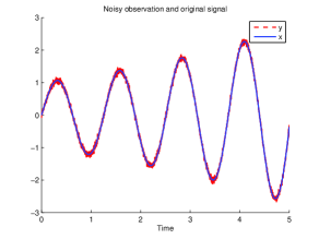
Figure 1: Signal $x$ and noisy signal $y$.

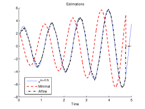
Figure 2: $\tilde{y}^{(0.5)}_{{t_{0}}}(0,0,T)$ with $T=0.25$ and $\tilde{y}^{(0.5)}_{{t_{0}}}(0,0,T,0.5)$ with $T=0.26$.

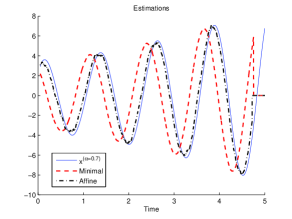
Figure 3: $\tilde{y}^{(0.7)}_{{t_{0}}}(0,0,T)$ with $T=0.25$ and $\tilde{y}^{(0.7)}_{{t_{0}}}(0,0,T,0.7)$ with $T=0.28$.

IV NUMERICAL SIMULATIONS

In order to show the efficiency and the stability of the proposed fractional order differentiators, we give some numerical results in this section.

We assume that $y(t_{i})=x(t_{i})+\varpi(t_{i})$ is the discrete noisy observation of $x$ on $I=[0,4]$ where $x(t_{i})=\exp(0.2t_{i})\sin(5t_{i})$, $\varpi$ is a zero-mean white Gaussian noise, and $t_{i}=T_{s}i$ for $i=0,\cdots,4\times 10^{3}$ with $T_{s}=\frac{1}{10^{3}}$. The variance of $\varpi$ is adjusted in such a way that the signal-to-noise ratio $SNR=10\log_{10}\left(\frac{\sum|y(t_{i})|^{2}}{\sum|\varpi(t_{i})|^{2}}\right)$ is equal to $SNR=28.07\text{dB}$. We can see the original signal $x$ and its noisy observation $y$ in Figure 1. The exact Jumarie’s modified Riemann-Liouville derivative of $x$ can be calculated by using (12), (11) and the Riemann-Liouville derivative of the functions $\sin(\cdot)$ and $\exp(\cdot)$ (see [29], p. 83). We estimate the derivatives $x^{(\alpha)}$ with $\alpha=0.5$ and $0.7$ respectively. We apply the trapezoidal numerical integration method to approximate the integrals in our differentiators where we use $m+1$ ($T=mT_{s}$) discrete observation values in each sliding integration window.

The formal derivatives and their estimated values are shown in Figure 2 and Figure 3, where the parameters $k$ and $\mu$ are set to zero for the Jacobi fractional differentiators. On one hand, the error due to the noise for the minimal Jacobi fractional differentiator can be negligible with respect to the truncated error part which produces a time-shift in the estimate. On the other hand, the noise error for the affine Jacobi fractional differentiator is larger than the one for the minimal Jacobi fractional differentiator, but the truncated error part is much smaller. Hence, the time-shift is significant reduced.

V CONCLUSION

In this paper, two non-asymptotic fractional order differentiators called minimal and affine Jacobi fractional differentiators are proposed by applying an algebraic parametric method to truncated expansions of fractional Taylor series. They can be used to estimate the recently invented Jumarie’s modified Riemann-Liouville derivative. Numerical simulations are given so as to show their efficiency and stability with respect to corrupting noises. It is shown that these differentiators can also be obtained by using the classical orthogonal properties of the Jacobi polynomials [21]. By using this method, a generalized affine Jacobi fractional differentiator will be obtained from a truncated fractional Taylor series expansion with an arbitrary truncated order in the future work. Moreover, in a similar way to [21] and [22], the noise errors and the truncated errors in these differentiators will be analyzed. In particular, we will study the influence of the parameters $k$, $\mu$ and $T$ to these errors so as to give a guideline for choosing the optimal parameters.

References

- [1] M. Abramowitz and I.A. Stegun, editeurs. Handbook of mathematical functions. GPO, 1965.
- [2] D.L. Chen, Y.Q. Chen and D.Y. Xue: Digital Fractional Order Savitzky-Golay Differentiator, IEEE Transactions on Circuits and Systems II: Express Briefs, 58, 11, pp. 758-762, 2011.
- [3] M. Cugnet, J. Sabatier, S. Laruelle, S. Grugeon, B. Sahut, A. Oustaloup and J.M. Tarascon: On Lead-acid battery resistance and cranking capability estimation, IEEE Transactions on Industrial Electronics, 57, 3, pp. 909-917, 2010.
- [4] M. Fliess and R. Hotzel: Sur les systèmes linéaires à dérivation non entière. C.R. Acad. Sci. Paris Ser. IIb, (signal, informatique), 324, pp. 99-105, 1997.
- [5] M. Fliess: Analyse non standard du bruit, C.R. Acad. Sci. Paris Ser. I, 342, pp. 797-802, 2006.
- [6] M. Fliess: Critique du rapport signal à bruit en communications numériques – Questioning the signal to noise ratio in digital communications, International Conference in Honor of Claude Lobry, Revue africaine d’informatique et de Mathématiques appliquées, 9, pp. 419-429, 2008.
- [7] M. Fliess and H. Sira-Ramírez: An algebraic framework for linear identification, ESAIM Control Optim. Calc. Variat., 9, pp. 151-168, 2003.
- [8] M. Fliess and H. Sira-Ramírez: Closed-loop parametric identification for continuous-time linear systems via new algebraic techniques, in H. Garnier, L. Wang (Eds): Identification of Continuous-time Models from Sampled Data, pp. 363-391, Springer, 2008.
- [9] M. Fliess, M. Mboup, H. Mounier and H. Sira-Ramírez: Questioning some paradigms of signal processing via concrete examples, in Algebraic Methods in Flatness, Signal Processing and State Estimation, H. Sira-Ramírez, G. Silva-Navarro (Eds.), Editiorial Lagares, México, pp. 1-21, 2003.
- [10] M. Fliess, C. Join, M. Mboup and H. Sira-Ramírez: Compression différentielle de transitoires bruités. C.R. Acad. Sci., I(339), pp. 821-826, Paris, 2004.
- [11] G.H. Hardy: A course of pure mathematics. Cambridge University Press, tenth edition, 1952.
- [12] R. Hotzel and M. Fliess: On linear systems with a fractional derivation: Introductory theory with examples. Mathematics and computers in Simulation, 45, pp. 385-395, 1998.
- [13] G. Jumarie: Modified Riemann-Liouville derivative and fractional Taylor series of nondifferentiable functions further results, Comput. Math. Appl. 51, pp. 1367-1376, 2006.
- [14] G. Jumarie: Table of some basic fractional calculus formulae derived from a modified Riemann-Liouville derivative for non-differentiable functions, Appl. Math. Lett. 22, pp. 378-385 2009.
- [15] G. Jumarie: Fourier’s transform of fractional order via Mittag-Leffler function and modified Riemann-Liouville derivative, J. Appl. Math. Inform. 26, pp. 1101-1121, 2008.
- [16] G. Jumarie: Laplac’s transform of fractional order via the Mittag-Leffler function and modified Riemann-Liouville derivative, Appl. Math. Lett. 22, pp. 1659-1664, 2009.
- [17] A.A. Kilbas, H.M. Srivastava, and J.J. Trujillo: Theory and Applications of Fractional Differential Equations, vol. 204 of North-Holland Mathematics Studies, Elsevier, Amsterdam, The Netherlands, 2006.
- [18] D.Y. Liu, O. Gibaru, W. Perruquetti, M. Fliess and M. Mboup: An error analysis in the algebraic estimation of a noisy sinusoidal signal. In: 16th Mediterranean conference on Control and automation (MED’08), Ajaccio, France, 2008.
- [19] D.Y. Liu, O. Gibaru and W. Perruquetti: Parameters estimation of a noisy sinusoidal signal with time-varying amplitude. In: 19th Mediterranean conference on Control and automation (MED’11), Corfu, Greece, 2011.
- [20] D.Y. Liu, O. Gibaru and W. Perruquetti: Error analysis for a class of numerical differentiator: application to state observation, 48th IEEE Conference on Decision and Control, Shanghai, China, 2009.
- [21] D.Y. Liu, O. Gibaru and W. Perruquetti: Differentiation by integration with Jacobi polynomials. J. Comput. Appl. Math., 235, 9, pp. 3015-3032, 2011.
- [22] D.Y. Liu, O. Gibaru and W. Perruquetti: Error analysis of Jacobi derivative estimators for noisy signals. Numerical Algorithms, 58, 1, pp. 53-83, 2011.
- [23] D.Y. Liu, O. Gibaru and W. Perruquetti: Convergence Rate of the Causal Jacobi Derivative Estimator. Curves and Surfaces 2011, LNCS 6920 proceedings, pp. 45-55, 2011.
- [24] A. Loverro: Fractional calculus, history, definitions and applications for the engineer. Rapport technique, Univeristy of Notre Dame: Department of Aerospace and Mechanical Engineering, May 2004.
- [25] J.A.T. Machado: Calculation of fractional derivatives of noisy data with genetic algorithms, Nonlinear Dyn., 57, 1/2, pp. 253-260, Jul. 2009.
- [26] M. Mboup: Parameter estimation for signals described by differential equations, Applicable Analysis, 88, pp. 29-52, 2009.
- [27] M. Mboup, C. Join and M. Fliess: A revised look at numerical differentiation with an application to nonlinear feedback control. In: 15th Mediterranean conference on Control and automation (MED’07). Athenes, Greece, 2007.
- [28] M. Mboup, C. Join and M. Fliess: Numerical differentiation with annihilators in noisy environment, Numerical Algorithms 50, 4, pp. 439-467, 2009.
- [29] K.S. Miller and B. Ross, An Introduction to the Fractional Calculus and Fractional Differential Equations, Wiley, New York, 1933.
- [30] A. Neves, M. Mboup and M. Fliess: An Algebraic Receiver for Full Response CPM Demodulation, VI International Telecommunications Symposium (ITS2006), September 3-6, Fortaleza-ce, Brazil, 2006.
- [31] A. Neves, M.D. Miranda and M. Mboup: Algebraic parameter estimation of damped exponentials, Proc. 15th Europ. Signal Processing Conf. - EUSIPCO 2007, Poznań, 2007.
- [32] K.B. Oldham and J. Spanier: The Fractional Calculus, Academic Press, New York 1974.
- [33] A. Oustaloup, B. Mathieu and P. Lanusse: The CRONE control of resonant plants : application to a flexible transmission, European Journal of Control, 1, 2, pp. 113-121, 1995.
- [34] A. Oustaloup, J. Sabatier and X. Moreau: From fractal robustness to the CRONE approach, ESAIM: Proceedings, pp. 177-192, Dec. 1998.
- [35] A. Oustaloup, J. Sabatier and P. Lanusse: From fractal robustness to the CRONE control, FCAA, 1, 2, pp. 1-30, Jan. 1999.
- [36] I. Podlubny: Fractional Differential Equations, vol. 198 of Mathematics in Science and Engineering, Academic Press, New York, NY, USA, 1999.
- [37] V. Pommier, J. Sabatier, P. Lanusse and A. Oustaloup: CRONE control of a nonlinear hydraulic actuator, Control Engineering Practice, 10, pp. 391-402, Jan. 2002.
- [38] S. Riachy, M. Mboup and J.P. Richard: Multivariate numerical differentiation. J. Comput. Appl. Math., 236, 6, pp. 1069-1089, 2011.
- [39] S. Riachy, Y. Bachalany, M. Mboup, and J.P. Richard: An algebraic method for multi-dimensional derivative estimation. In: 16th Mediterranean conference on Control and automation (MED’08), Ajaccio, France, 2008.
- [40] S. Riachy, Y. Bachalany, M. Mboup and J.P. Richard: Différenciation numérique multivariable I: estimateurs algébriques et structure, in: 6ieme Confrence Internationale Francophone d’Automatique, 2010.
- [41] J.R. Trapero, H. Sira-Ramírez and V.F. Battle: An algebraic frequency estimator for a biased and noisy sinusoidal signal, Signal Processing, 87, pp. 1188-1201, 2007.
- [42] R. Ushirobira, W. Perruquetti, M. Mboup and M. Fliess: Estimation algébrique des paramètres intrinsèques d’un signal sinusoïdal biaisé en environnement bruité, XXIIIe Colloque Gretsi, Bordeaux, France, 2011.
- [43] G.C. Wu and E.W.M. Lee: Fractional Variational Iteration method and Its Appliation, Phys. Lett. A 374, pp. 2506- 2509, 2010.
- [44] Y. Tian, T. Floquet and W. Perruquetti, Fast state estimation in linear time-varying systems: an algebraic approach, 47th IEEE Conference on Decision and Control, Cancun, Mexique, 2008.