Vector coherent state representations and their inner products

Abstract

Several advances have extended the power and versatility of coherent state theory to the extent that it has become a vital tool in the representation theory of Lie groups and their Lie algebras. Representative applications are reviewed and some new developments are introduced. The examples given are chosen to illustrate special features of the scalar and vector coherent state constructions and how they work in practical situations. Comparisons are made with Mackey’s theory of induced representations. For simplicity, we focus on square integrable (discrete series) unitary representations although many of the techniques apply more generally, with minor adjustment.

PACS numbers: 02.20.–a, 02.20.Sv, 21.60.Fw, 21.60.Ev

Published in J. Phys. A: Math, Theor. 45 (2012) 24003

1 Introduction

Coherent state theory is known to reveal classical behaviour in quantum mechanics. Thus, it has been used extensively in studying the relationship between classical and quantum mechanics and in the development of quantization techniques [1, 2, 3, 4, 5]. The applications of coherent state theory outlined in this paper facilitate the quantisation of an algebraic system by construction of the unitary representations of its spectrum generating algebra.

Standard coherent state representations, which we refer to as scalar coherent state representations, were introduced by Bargmann [6] and Segal [7] and defined more generally by Perelomov [8], Onofri [9], and others. They were subsequently extended to vector-valued coherent state (VCS) representations [10, 11, 12] and used widely in the construction of explicit representations of many Lie algebras and Lie groups [13, 14, 15, 16, 17]. Early applications were reviewed in a book by Hecht [18]. A new class of representations was introduced for representations on functions of SO(3) [19, 20, 21, 22] which were later used in the construction of shift tensors [23], and for the computation of Clebsch-Gordan coefficients for reducing tensor product representations [24, 25, 26]. VCS theory was, in fact, designed for the specific purpose of inducing the harmonic series of irreps (irrreducible representations) of the non-compact symplectic Lie algebra $\mbox{\lfrak sp}(3,\mathbb{R})$ from those of its maximal compact u(3) subalgebra [27, 11, 12, 10]. These irreps are needed in applications of the microscopic nuclear collective model [28, 29, 30].

It has been shown [31] that VCS theory is a physically intuitive theory of induced representations [32] with the advantage that the representations it induces are irreducible. It is also known [33, 34] that scalar and VCS representations relate closely to those of geometric quantization [35, 36, 37] and, in some respects, extend them.

In this review, we restrict consideration to applications of scalar and VCS theory to the construction of unitary irreps of Lie algebras. Several examples are used to illustrate the different ways and the much larger variety of representations that can be induced by the extension to vector-valued wave functions. The construction of a VCS representation is straightforward. The more challenging part is to determine an orthonormal basis for its Hilbert space and calculate the matrix elements required for the application of spectrum generating algebras in quantum physics. For this purpose, VCS theory relies on K-matrix theory [10, 31, 38]. K-matrix theory (distinct from K-theory as used in mathematics) provides practical procedures for determining the inner products of coherent state and VCS representations as shown, in the context in which it is used, in this review. It is an essential component of VCS theory, although it can be used more generally. It could be used, for example, to compute matrix elements of a unitary representation from those obtained by the partial-coherent-state methods of Deenen and Quesne [39]. K-matrix theory is developed in Sect. 6.

In approaching coherent-state representation theory as a theory of quantisation, it is useful to recognise that a Schrödinger representation of state vectors in quantum mechanics by wave functions is, in fact, a coherent state representation. This is explained in Section 7.

2 Scalar coherent state representation

Many definitions of coherent states and coherent state representations have been given [40, 8, 41] and are described in several reviews [1, 42, 43]. Following Perelomov [42], we start with a basic definition but quickly adjust it to one that is more useful.

2.1 Basic coherent state representations

Let $\hat{T}$ denote a unitary irrep of a Lie group $G$ on a Hilbert space $\mathbf{H}$ with inner product of two vectors $|\psi\rangle$ and $|\varphi\rangle$ denoted by $\langle\psi|\varphi\rangle$. Then, for any normalised vector $|\phi\rangle\in\mathbf{H}$ (known as a fiducial vector), a system of coherent state vectors for the irrep is defined as the set

$$\mathfrak{M}_{\phi}:=\{|\phi(g)\rangle=\hat{T}(g)|\phi\rangle;g\in G\}.$$ (1)

The vectors in $\mathfrak{M}_{\phi}$ span the Hilbert space $\mathbf{H}$. Thus, in a coherent-state representation, an arbitrary vector $|\psi\rangle\in\mathbf{H}$ can be assigned a wave function, $\Psi$, defined on the group $G$ by the overlaps

$$\Psi(g):=\langle\phi|\hat{T}(g)|\psi\rangle,\quad g\in G.$$ (2)

The space spanned by these wave functions, $\mathcal{H}$, carries a coherent-state irrep $\hat{\Gamma}$, that is isomorphic to $\hat{T}$ and defined by

$$\hat{\Gamma}(g)\Psi(g^{\prime}):=\langle\phi|\hat{T}(g^{\prime})\hat{T}(g)|\psi\rangle=\Psi(g^{\prime}g),\quad\forall\,g,g^{\prime}\in G.$$ (3)

Thus, $\mathcal{H}$ is a Hilbert space with inner product inherited from the map $\mathbf{H}\to\mathcal{H};|\psi\rangle\mapsto\Psi$.

When $G$ is compact, and for some (e.g., discrete series) representations when $G$ is non-compact, the inner product for $\mathcal{H}$ is is defined by the so-called resolution of the identity operator

$$\hat{\mathcal{I}}:=\int_{G}T^{\dagger}(g)|\phi\rangle\langle\phi|T(g)\,dV(g),$$ (4)

where $dV(g)$ is a right $G$-invariant volume element. Because $\hat{T}$ is unitary, we have the equality

$$\hat{\mathcal{I}}\,\hat{T}(\alpha)=\hat{T}(\alpha)\,\hat{\mathcal{I}},\quad\forall\,\alpha\in G.$$ (5)

Therefore, by Schur’s lemma, $\hat{\mathcal{I}}$ is a multiple of the identity and, with a suitable normalisation of the volume element $dV$,

$$\int_{G}\Psi^{*}(g)\Phi(g)\,dV(g)=\int_{G}\langle\phi|\hat{T}^{\dagger}(g)|\phi\rangle\langle\phi|\hat{T}(g)|\psi\rangle\,dV(g)=\langle\psi|\varphi\rangle.$$ (6)

2.2 More general coherent state representations

The above coherent state representations are defined on Hilbert spaces of complex-valued functions for any choice of fiducial vector, $|\phi\rangle$. However, a judicious choice of $|\phi\rangle$ can result in major simplifications. In particular, it is known [42, 1] that, for some choices, it is possible to identify systems of coherent states vectors with simpler properties, that also span the Hilbert space and give rise to more useful coherent state realisations of a given irrep. Moreover, as we illustrate, evaluation of the inner products for the corresponding coherent state wave functions by algebraic K-matrix methods can also become much easier and apply more generally (particularly for irreps of non-compact groups for which the above resolution of the identity does not satisfy the required convergence conditions).

Assume that the representation $\hat{T}$ has an extension to a representation of $G^{\mathbb{C}}$, the complex extension of $G$, defined by the natural complex extension of the Lie algebra of $G$. Let $|\phi\rangle$ be a fiducial vector and let $N$ be a subset of $G^{c}$ such that the coherent-state vectors

$$\{\hat{T}^{\dagger}(z)|\phi\rangle;z\in N\}$$ (7)

span $\mathbf{H}$. Then, any vector $|\psi\rangle\in\mathbf{H}$ is uniquely defined by the coherent state wave functions

$$\Psi(z):=\langle\phi|\hat{T}(z)|\psi\rangle,\quad\forall\,z\in N,$$ (8)

and a coherent state representation of $G$ is defined by

$$\hat{\Gamma}(g)\Psi(z):=\langle\phi|\hat{T}(z)\hat{T}(g)|\psi\rangle,\quad\forall\,g\in G.$$ (9)

Such a coherent state representation is an induced representation. For, if $H\subset G$ denotes the isotropy subgroup of all elements $h\in G$ for which

$$\hat{T}(h)|\phi\rangle=\sigma(h)|\phi\rangle,\quad{\rm with}\;\sigma(h)\in\mathbb{C}.$$ (10)

the map $\sigma:H\to\mathbb{C};h\mapsto\sigma(h)$ is the one-dimensional unitary representation of $H$ from which the coherent state irrep $\hat{\Gamma}$ is induced. And, as in standard induced representation theory [32], the wave functions of the induced representation satisfy the symmetry condition

$$\Psi(hz):=\langle\phi|\hat{T}(h)\hat{T}(z)|\psi\rangle=\sigma(h)\Psi(z),\quad\forall\,z\in N,\;h\in H.$$ (11)

2.3 Holomorphic coherent state representations of su(1,1)

Holomorphic coherent state representations can be constructed for both compact and non-compact semi-simple Lie groups and their Lie algebras. However, the unitary irreps of non-compact groups are usually of infinite dimension, for which extra considerations apply. For example, whereas the irreps of compact semi-simple and reductive Lie groups have both highest and lowest weights, those of a non-compact group may have a highest or a lowest weight but, generally, not both. A more essential distinction is that if $\{\hat{X}^{+}_{i}\}$ is a set of raising operators, relative to a lowest weight state $|\phi\rangle$ for an irrep of a non-compact Lie group, the values of $\{z_{i}\}$ required to define a set of coherent state vectors

$$\{|\phi(z)\rangle:=\exp(\sum_{i}z_{i}^{*}\hat{X}^{+}_{i})|\phi\rangle,z_{i}\in\mathbb{C}\},$$ (12)

that span the Hilbert space for the irrep, can be restricted to a subset. For a compact Lie group no such restriction is necessary because the expansion of the exponential for $|\phi(z)\rangle$ in this set terminates when a highest weight vector is reached. However, when there is no highest weight state, the expansion does not terminate. Then, for some values of the $z_{i}$ variables, $|\phi(z)\rangle$ may not converge to a normalisable vector in the Hilbert space. Thus, the domains of the complex variables $\{z_{i}\}$ are appropriately restricted to give subsets of normalisable vectors, i.e., subsets for which

$$\langle\phi(z)|\phi(z)\rangle<\infty.$$ (13)

As we now find, this complication is not much in evidence in the construction of the coherent state representation of the Lie algebra, but it has important consequences for the inner product for the Hilbert space of coherent state wave functions and their inner products (see Sect. 6).

We consider a unitary irrep $\hat{T}$ of su(1,1) with lowest weight. The su(1,1)^C Lie algebra, is spanned by a Cartan element $S_{0}$ and a pair of raising and lowering operators $S_{\pm}$ that satisfy the commutation relations

$$[S_{0},S_{\pm}]=\pm S_{\pm},\quad[S_{-},S_{+}]=2S_{0}.$$ (14)

Let $|\lambda 0\rangle$ denote a lowest weight state for an su(1,1) irrep that is annihilated by $\hat{S}_{-}:=\hat{T}(S_{-})$ and is an eigenstate of $\hat{S}_{0}:=\hat{T}(S_{0})$, so that

$$\hat{S}_{-}|\lambda 0\rangle=0,\quad 2\hat{S}_{0}|\lambda 0\rangle=\lambda|\lambda 0\rangle.$$ (15)

A state $|\psi\rangle$ in the Hilbert space of this irrep then has a holomorphic coherent state wave function with values

$$\Psi^{(\lambda)}(z)=\langle\lambda 0|e^{z\hat{S}_{-}}|\psi\rangle,$$ (16)

with $z$ restricted to values for which Eqn. (13) is satisfied. The coherent state representation $\hat{\Gamma}^{(\lambda)}$ of the su(1,1) algebra on these wave functions is then defined by

$$\hat{\Gamma}^{(\lambda)}(X)\Psi^{(\lambda)}(z):=\langle\lambda 0|e^{z\hat{S}_{-}}\hat{X}|\psi\rangle,\quad{\rm for}\;X\in\mbox{\lfrak su}(1,1)^{\mathbb{C}}.$$ (17)

Thus, if $\hat{\mathcal{S}}^{(\lambda)}_{0}:=\hat{\Gamma}^{(\lambda)}(S_{0})$ and $\hat{\mathcal{S}}^{(\lambda)}_{\pm}:=\hat{\Gamma}^{(\lambda)}(S_{\pm})$, we obtain

$$\hat{\mathcal{S}}^{(\lambda)}_{-}\Psi(z)=\langle\lambda 0|e^{z\hat{S}_{-}}\hat{S}_{-}|\psi\rangle=\langle\lambda 0|\hat{S}_{-}e^{z\hat{S}_{-}}|\psi\rangle,$$ (18)

$$\hat{\mathcal{S}}^{(\lambda)}_{0}\Psi(z)=\langle\lambda 0|e^{z\hat{S}_{-}}\hat{S}_{0}|\psi\rangle=\langle\lambda 0|\big{[}\hat{S}_{0}+z\hat{S}_{-}\big{]}e^{z\hat{S}_{-}}|\psi\rangle,$$ (19)

$$\hat{\mathcal{S}}^{(\lambda)}_{+}\Psi(z)=\langle\lambda 0|e^{z\hat{S}_{-}}\hat{S}_{+}|\psi\rangle=\langle\lambda 0|\big{[}\hat{S}_{+}+2z\hat{S}_{0}+z^{2}\hat{S}_{-}\big{]}e^{z\hat{S}_{-}}|\psi\rangle,$$ (20)

and the coherent state representation

$$\hat{\mathcal{S}}^{(\lambda)}_{-}=\frac{\partial}{\partial z},\quad\hat{\mathcal{S}}^{(\lambda)}_{0}=\frac{1}{2}\lambda+z\frac{\partial}{\partial z},\quad\hat{\mathcal{S}}^{(\lambda)}_{+}=z\Big{(}\lambda+z\frac{\partial}{\partial z}\Big{)}.$$ (21)

It is seen that the coherent state wave function for the lowest weight state is the constant function $\Psi_{\lambda 0}(z)=1$ and that the raising operator increases the degree of a wave function by one. Thus, in an elementary application of K-matrix methods, an orthonormal basis of coherent-state wave functions, $\{\Psi_{\lambda n}\}$, is given for the irrep $T^{(\lambda)}$ by

$$\Psi_{\lambda n}(z):=K_{\lambda n}\,z^{n},\quad n=0,1,2,\dots$$ (22)

with norm factors that remain to be determined. It follows that

$$\displaystyle\hat{\mathcal{S}}^{(\lambda)}_{+}\Psi_{\lambda n}(z)=K_{\lambda n}(\lambda+n)z^{n+1}=(\lambda+n)\frac{K_{\lambda n}}{K_{\lambda,n+1}}\,\Psi_{\lambda,n+1}(z),$$ (23)

$$\displaystyle\hat{\mathcal{S}}^{\lambda)}_{-}\Psi_{\lambda,n+1}(z)=(n+1)\frac{K_{\lambda,n+1}}{K_{\lambda n}}\Psi_{\lambda n}(z),$$ (24)

$$\displaystyle\hat{\mathcal{S}}^{(\lambda)}_{0}\Psi_{\lambda n}(z)=\textstyle\big{(}\frac{1}{2}\lambda+n\big{)}\Psi_{\lambda n}(z).$$ (25)

The norm factors are then determined in K-matrix theory by requiring the matrices of the su(1,1) representation to satisfy the Hermiticity relationships,

$$\langle{\lambda,n+1}|\hat{{S}}_{+}|{\lambda n}\rangle=\langle{\lambda n}|\hat{{S}}_{-}|{\lambda,n+1})^{*},$$ (26)

$$\langle{\lambda n}|\hat{{S}}_{0}|{\lambda n}\rangle=\langle{\lambda n}|\hat{{S}}_{0}|{\lambda n}\rangle^{*},$$ (27)

required of a unitary irrep. To satisfy Eqn. (26), it is required that

$$\left|\frac{K_{\lambda,n+1}}{K_{\lambda n}}\right|^{2}=\frac{\lambda+n}{n+1}.$$ (28)

Equation (27) is then also satisfied and we obtain the standard expressions

$$\hat{\mathcal{S}}_{0}\Psi_{\lambda n}(z)=\textstyle\big{(}\frac{1}{2}\lambda+n\big{)}\Psi_{\lambda n}(z),$$ (29)

$$\hat{\mathcal{S}}_{+}\Psi_{\lambda n}=\sqrt{(\lambda+n)(n+1)}\,\Psi_{\lambda,n+1},$$ (30)

$$\hat{\mathcal{S}}_{-}\Psi_{\lambda,n+1}=\sqrt{(\lambda+n)(n+1))}\,\Psi_{\lambda n}.$$ (31)

If needed, the recursion relation (28) for $K_{\lambda n}$ is easily solved with $K_{\lambda 0}=1$ to give

$$K_{\lambda n}=\sqrt{\frac{(\lambda+n-1)!}{(\lambda-1)!\,n!}}$$ (32)

and the orthonormal basis of coherent-state wave functions

$$\Psi_{\lambda n}(z)=\sqrt{\frac{(\lambda+n-1)!}{(\lambda-1)!\,n!}}\,z^{n},\quad n=0,1,2,\dots\,.$$ (33)

2.4 An SO(3) coherent state representations of su(3)

The scalar holomorphic coherent state representations of reductive and semi-simple Lie groups and algebras, considered above, have proved to be useful and insightful in numerous applications. However, there are other possibilities and, for practical purposes, some that are more useful. For SU(3), for example, the scalar holomorphic representations are limited to a subset of irreps in a canonical SU(2) basis, whereas in physical applications, especially in nuclear physics, one needs the full set of irreps in an SO(3)-coupled basis. Such coherent state irreps are readily constructed [19, 20] from the observation that, provided a highest weight state $|\lambda\mu\rangle$ for the desired SU(3) irrep $\hat{T}^{(\lambda\mu)}$ is not an eigenstate of any component of the so(3) angular momentum algebra, a complete set of SO(3) coherent states, i.e., a set that spans the SU(3) irrep of highest weight $(\lambda\mu)$, is given by the set

$$\{\hat{T}^{(\lambda\mu)}(\Omega)|\lambda\mu\rangle,\;\Omega\in{\rm SO}(3)\}.$$ (34)

We show in the following sections that complete sets of SU(3) irreps, in both canonical SU(2) and SO(3) bases, are given more usefully in VCS theory.

3 Vector coherent state (VCS) representation

A VCS irrep is an irrep of a Lie group $G$ that is induced from a multi-dimensional irrep of a subgroup by generalising the coherent state construction to vector-valued wave functions. Vector-valued coherent state methods [27, 10, 11] and related partial coherent-state methods [39] were introduced for the non-compact Sp$(n,\mathbb{R})$ symplectic groups in 1984. In fact, holomorphic vector-valued representations of the Sp$(n,\mathbb{R})$ groups had been constructed many years previously by Harish-Chandra [44]. However, they were not used in physics because of the intractable nature of their inner products. This obstacle was resolved, within the framework of VCS theory, by algebraic K-matrix methods [10, 38] which by-pass the need for carrying out the computationally intensive integrals of the Harish-Chandra inner products [45, 46]. They were nevertheless shown [12] to give the same results. An early review of VCS theory and its applications was given by Hecht [18].

Basic VCS irreps are defined as follows. Let $\hat{\sigma}$ denote a unitary irrep of a subgroup $H\subset G$ and suppose that this irrep is realised in the restriction of a unitary irrep $\hat{T}$ of $G$ to $H$. This means that the Hilbert space, $\mathbf{H}$, for the irrep $\hat{T}$ of $G$, contains a subspace $\mathbf{H}_{0}\subset\mathbf{H}$ that is $H$-invariant, i.e.,

$$\hat{T}(h)|\phi\rangle\in\mathbf{H}_{0},\quad\forall\,h\in H\;{\rm and}\;\forall|\phi\rangle\in\mathbf{H}_{0},$$ (35)

and that this subspace is irreducible and equivalent to $\hat{\sigma}$ under the restriction of $\hat{T}$ to $H$. Moreover, it is possible to choose an orthonormal basis, $\{|\nu\rangle\}$ for $\mathbf{H}_{0}$ in such a way that the operator

$$\hat{\Pi}:=\sum_{\nu}\xi_{\nu}\langle\nu|$$ (36)

intertwines the representation $\hat{\sigma}$ and the irrep $\hat{T}(H)$ on $\mathbf{H}_{0}$, i.e.,

$$\hat{\Pi}\hat{T}(h)=\hat{\sigma}(h)\hat{\Pi},\quad\forall\,h\in H,$$ (37)

A vector $|\psi\rangle\in\mathbf{H}$ can now be represented by a vector-valued wave function

$$\Psi(g):=\hat{\Pi}\hat{T}(g)|\psi\rangle=\sum_{\nu}\xi_{\nu}\langle\nu|\hat{T}(g)|\psi\rangle,\quad g\in G,$$ (38)

which satisfies the identity

$$\Psi(hg)=\hat{\sigma}(h)\Psi(g),\quad\forall\,h\in H,\;{\rm and}\;\forall\,g\in G.$$ (39)

The Hilbert space of such VCS wave functions, $\mathcal{H}$, carries a coherent-state irrep $\hat{\Gamma}$, induced from the irrep $\hat{\sigma}$ of $H$, which is isomorphic to $\hat{T}$ and defined by

$$\hat{\Gamma}(g)\Psi(g^{\prime}):=\Psi(g^{\prime}g),\quad\forall\,g,g^{\prime}\in G.$$ (40)

Thus, $\mathcal{H}$ has an inner product inherited from the map $\mathbf{H}\to\mathcal{H};|\psi\rangle\mapsto\Psi$. When $G$ is compact, and for some (e.g., discrete series) representations when $G$ is non-compact, the inner product for $\mathcal{H}$ is defined by the resolution of the identity operator

$$\hat{\mathcal{I}}:=\int_{G}\sum_{\mu\nu}T^{\dagger}(g)|\mu\rangle\xi_{\mu}^{\dagger}\cdot\xi_{\nu}\langle\nu|T(g)\,dV(g),$$ (41)

where $dV(g)$ is a right $G$-invariant volume element. Because $\hat{T}$ is unitary, we then have the equality

$$\hat{\mathcal{I}}\,\hat{T}(\alpha)=\hat{T}(\alpha)\,\hat{\mathcal{I}},\quad\forall\,\alpha\in G.$$ (42)

Therefore, by Schur’s lemma, $\hat{\mathcal{I}}$ is a multiple of the identity. Thus, if $\Psi$ and $\Phi$ are, respectively, VCS wave functions for vectors $|\psi\rangle$ and $|\phi\rangle$ in $\mathbf{H}$, defined as vector-valued functions over $G$ by Eqn. (38), it follows that, with a suitable normalisation of the volume element $dV$,

$$\int_{G}\Psi^{\dagger}(g)\cdot\Phi(g)\,dV(g) = \int_{G}\sum_{\mu\nu}\langle\psi|T^{\dagger}(g)|\mu\rangle\xi_{\mu}^{\dagger}\cdot\xi_{\nu}\langle\nu|T(g)|\phi\rangle\,dV(g)$$ (43)

$$= \langle\psi|\varphi\rangle.$$

The above definition of a VCS irrep is useful for formal purposes, but in practice VCS wave function are defined more usefully and more generally in terms of a subgroup or subset $N\subset G^{\mathbb{C}}$ such that, if the subspace $\mathbf{H}_{0}\subset\mathbf{H}$ is of dimension $d$, the coherent state vectors

$$\{\hat{T}^{\dagger}(z)|\nu_{i}\rangle;z\in N,\;i=1,\dots,d\}$$ (44)

span $\mathbf{H}$. The construction then parallels that given above except that K-matrix methods are required, as for scalar coherent state representations, to evaluate inner products.

4 Holomorphic VCS irreps of the u(3) Lie algebra

The construction of holomorphic irreps of the u(3) Lie algebra by VCS methods serves as a prototype for parallel constructions for other semi-simple and reductive Lie algebras. A simple application of the holomorphic VCS construction to a Lie algebra g, requires that the complex extension, $\mbox{\lfrak g}^{\mathbb{C}}$, of g can be expressed as a vector space sum of the complex extension of a compact subalgebra $\mbox{\lfrak h}\subset\mbox{\lfrak g}$ plus Abelian subalgebras, $\mbox{\lfrak n}_{\pm}$, of raising and lowering operators, i.e.,

$$\mbox{\lfrak g}^{\mathbb{C}}=\mbox{\lfrak h}^{\mathbb{C}}\oplus\mbox{\lfrak n}_{+}\oplus\mbox{\lfrak n}_{-}.$$ (45)

The only classical Lie algebras for which this is not always possible are those of the odd orthogonal groups SO$(2n+1)$, for which more general VCS constructions [14] are required. A practical limitation in the application of holomorphic VCS irreps arises because the expressions it gives for orthonormal bases and matrix elements are in terms of Clebsch-Gordan and Racah coefficients of the subalgebra h; these are currently only available for the semi-simple Lie algebras su(2), su(3) and so(4), and their reductive extensions, e.g., u(2) and u(3). Fortunately, this limitation did not exclude their application to the discrete series irreps of the non-compact symplectic Lie algebra $\mbox{\lfrak sp}(3,\mathbb{R})$, induced from those of its maximal compact subalgebra u(3) [27, 11, 10].

The complex extension, $\mbox{\lfrak u}(3)^{\mathbb{C}}$, of u(3) is the Lie algebra of all complex $3\times 3$ matrices. It is spanned by 9 matrices $\{C_{ij}\}$ with elements

$$(C_{ij})_{kl}=\delta_{i,k}\delta_{j,l}$$ (46)

and commutation relations

$$[C_{ij},C_{kl}]=\delta_{k,j}C_{il}-\delta_{i,l}C_{kj}.$$ (47)

The subset $\{C_{ii};i=1,2,3\}$ spans a Cartan subalgebra and the subsets $\{C_{ik};i<k\}$ and $\{C_{ik};i>k\}$ are, respectively, raising and lowering operators.

We consider a generic u(3) irrep, $\hat{T}^{(\lambda)}$, in which the matrices $\{C_{ij}\}$ are represented by operators, $\{\hat{C}_{ij}\}$, on a Hilbert space, $\mathbf{H}^{(\lambda)}$, with highest-weight $\lambda:=\{\lambda_{1}\lambda_{2}\lambda_{3}\}$, where $\lambda_{1}$, $\lambda_{2}$, and $\lambda_{3}$ differ by integers and satisfy the inequality $\lambda_{1}\geq\lambda_{2}\geq\lambda_{3}$. We then define a subspace $\mathbf{H}^{(\lambda)}_{0}\subset\mathbf{H}^{(\lambda)}$ of so-called highest-grade states, defined by

$$\mathbf{H}^{(\lambda)}_{0}:=\big{\{}|\psi\rangle\in\ \mathbf{H}^{(\lambda)}\,\big{|}\,\hat{C}_{12}|\psi\rangle=\hat{C}_{13}|\psi\rangle=0\big{\}}.$$ (48)

The isotropy subgroup, $H$, of all U(3) elements that leave $\mathbf{H}^{(\lambda)}_{0}$ invariant is then a group with Lie algebra, $\mbox{\lfrak h}=\mbox{\lfrak u}(1)\oplus\mbox{\lfrak u}(2)$, for which the complex extension is spanned by the zero and horizontal root vectors, $\{C_{11},C_{ik},i,k=2,3\}$, of the u(3) root diagram, shown in Fig. 1(a).

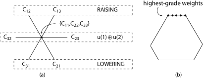
Figure 1: The root diagram for u(3), Fig. (a), and the boundary of the weight diagram for an irrep $\lambda:=\{\lambda_{1}\lambda_{2}\lambda_{3}\}$, Fig. (b). The Hermitian combinations of the horizontal root vectors span the isotropy subalgebra, $\mbox{\ftfrak h}=\mbox{\ftfrak u}(1)\!\,\oplus\!\,\mbox{\ftfrak u}(2)\!\subset\!\mbox{\ftfrak u}(3)$, of elements that leave invariant the space, $\mathbf{H}^{(\lambda)}_{0}$, spanned by the highest-grade vectors whose weights are shown.

The Hilbert space, $\mathbf{H}^{(\lambda)}_{0}$, carries a known irrep of the Lie algebra h. The elements

$$2S_{0}:=C_{22}-C_{33},\quad S_{+}:=C_{23},\quad S_{-}:=C_{32},$$ (49)

are standard basis elements for the complex extension of an su(2) subalgebra of h. Thus, $\mathbf{H}^{(\lambda)}_{0}$ is spanned by orthonormal basis vectors, $\{|(\lambda)sm\rangle\}$, for which

$$\hat{C}_{11}|(\lambda)sm\rangle=\lambda_{1}|(\lambda)sm\rangle,\quad\big{(}\hat{C}_{22}+\hat{C}_{33}\big{)}|(\lambda)sm\rangle=\big{(}\lambda_{2}+\lambda_{3}\big{)}|(\lambda)sm\rangle,$$ (50)

$$\hat{S}_{0}|(\lambda)sm\rangle=m|(\lambda)sm\rangle,$$ (51)

$$\hat{S}_{\pm}|(\lambda)sm\rangle=\sqrt{(s\mp m)(s\pm m+1)}|(\lambda)s,m\pm 1\rangle,$$ (52)

$$s=\textstyle\frac{1}{2}(\lambda_{2}-\lambda_{3}),\quad m=-s,-s+1,\dots,s.$$ (53)

Thus, the irrep of h carried by the highest-grade subspace $\mathbf{H}^{(\lambda)}_{0}\subset\mathbf{H}^{(\lambda)}$ is completely defined by the highest-weight $\lambda$.

In accordance with the principles outlined in Sect. 3, we now introduce intrinsic wave functions, $\{\xi^{(\lambda)}_{sm}\}$, for the states $\{|(\lambda)sm\rangle\}$ and a corresponding irrep, $\hat{\sigma}$, of the operators of h by intrinsic operators $\{\hat{\sigma}_{11},\hat{\sigma}_{ik},i,k=2,3\}$. Eqns. (50) - (53) then define corresponding transformations of these intrinsic wave functions:

$$\hat{\sigma}_{11}\xi^{(\lambda)}_{sm}=\lambda_{1}\xi^{(\lambda)}_{sm},\quad\big{(}\hat{\sigma}_{22}+\hat{\sigma}_{33}\big{)}\xi^{(\lambda)}_{sm}=\big{(}\lambda_{2}+\lambda_{3}\big{)}\xi^{(\lambda)}_{sm},$$ (54)

$$\hat{s}_{0}\xi^{(\lambda)}_{sm}=m\xi^{(\lambda)}_{sm},\quad\hat{s}_{\pm}\xi^{(\lambda)}_{sm}=\sqrt{(s\mp m)(s\pm m+1)}\xi^{(\lambda)}_{s,m\pm 1},$$ (55)

where

$$2\hat{s}_{0}:=\hat{\sigma}_{22}-\hat{\sigma}_{33},\quad\hat{s}_{+}:=\hat{\sigma}_{23},\quad\hat{s}_{-}:=\hat{\sigma}_{32},$$ (56)

A VCS irrep of u(3) of highest weight $\lambda$ is now induced from the irrep $\hat{\sigma}$ of h in parallel with the construction of a holomorphic scalar coherent state irrep. In this irrep, a vector $|\psi\rangle\in\mathbf{H}^{(\lambda)}$ is represented by a holomorphic vector-valued wave function

$$\Psi(z):=\sum_{m}\xi^{(\lambda)}_{sm}\langle{(\lambda)}sm|e^{\hat{Z}}|\psi\rangle,\quad\hat{Z}:=\sum_{k}z_{k}\hat{C}_{1k}.$$ (57)

The corresponding representation, $C_{\mu\nu}\to\hat{\mathcal{C}}^{(\lambda)}_{\mu\nu}\equiv\hat{\Gamma}^{(\lambda)}(C_{\mu\nu})$, of the u(3) Lie algebra, is then defined in the standard way by

$$\hat{\mathcal{C}}^{(\lambda)}_{\mu\nu}\Psi(z):=\sum_{m}\xi^{(\lambda)}_{sm}\langle{(\lambda)}sm|e^{\hat{Z}}\hat{C}^{(\lambda)}_{\mu\nu}|\psi\rangle.$$ (58)

Thus, with $i,k>1$ and the expansions

$$\hat{\mathcal{C}}^{(\lambda)}_{1i}\Psi(z)=\sum_{m}\xi{(\lambda)}_{sm}\langle{(\lambda)}{sm}|\hat{C}_{1i}e^{\hat{Z}}|\psi\rangle,$$ (59)

$$\hat{\mathcal{C}}^{(\lambda)}_{11}\Psi(z)=\sum_{m}\xi^{(\lambda)}_{sm}\langle{(\lambda)}{sm}|\big{[}\hat{C}_{11}-\!\sum_{k=2}^{3}z_{k}\hat{C}_{1k}\big{]}e^{\hat{Z}}|\psi\rangle,$$ (60)

$$\hat{\mathcal{C}}^{(\lambda)}_{ik}\Psi(z)=\sum_{m}\xi^{(\lambda)}_{sm}\langle{(\lambda)}{sm}|\big{[}\hat{C}_{ik}+z_{i}\hat{C}_{1k}\big{]}e^{\hat{Z}}|\psi\rangle,$$ (61)

$$\hat{\mathcal{C}}^{(\lambda)}_{i1}\Psi(z)=\sum_{m}\xi^{(\lambda)}_{sm}\langle{(\lambda)}{sm}|\big{[}z_{i}\hat{C}_{11}-\!\sum_{k=2}^{3}z_{k}\hat{C}_{ik}-z_{i}\sum_{k=2}^{3}z_{k}\hat{C}_{1k}\big{]}e^{\hat{Z}}|\psi\rangle,$$ (62)

we obtain

$$\hat{\mathcal{C}}^{(\lambda)}_{1i}=\partial_{i}:=\partial/\partial z_{i},$$ (63)

$$\hat{\mathcal{C}}^{(\lambda)}_{11}=\lambda_{1}-\!\sum_{k=2}^{3}z_{k}\partial_{k},\quad\hat{\mathcal{C}}^{(\lambda)}_{ik}=\hat{\sigma}_{ik}+z_{i}\partial_{k},$$ (64)

$$\hat{\mathcal{C}}^{(\lambda)}_{i1}=\lambda_{1}z_{i}-\sum_{k=2}^{3}\hat{\sigma}_{ik}z_{k}-z_{i}\sum_{k=2}^{3}z_{k}\partial_{k}.$$ (65)

Derivation of the operators of a VCS representation of any classical Lie algebra, except for the odd orthogonal algebras, is equally straightforward.

We now consider the determination of u(3) matrix elements in an orthonormal basis. This is simplified by use of SU(2) tensorial methods. With su(2) spin operators defined in terms of the VCS operators of Eqn. (64) by

$$2\hat{\mathcal{S}}^{(\lambda)}_{0}=\hat{\mathcal{C}}^{(\lambda)}_{22}-\hat{\mathcal{C}}^{(\lambda)}_{33},\quad\hat{\mathcal{S}}^{(\lambda)}_{+}=\hat{\mathcal{C}}^{(\lambda)}_{23},\quad\hat{\mathcal{S}}^{(\lambda)}_{-}=\hat{\mathcal{C}}^{(\lambda)}_{32},$$ (66)

it is determined that the $z_{2}$ and $z_{3}$ variables obey the commutation relations

$$[\hat{\mathcal{S}}^{(\lambda)}_{0},z_{2}]=\textstyle\frac{1}{2}z_{2},\quad[\hat{\mathcal{S}}^{(\lambda)}_{0},z_{3}]=\textstyle-\frac{1}{2}z_{3},$$ (67)

$${[}\hat{\mathcal{S}}^{(\lambda)}_{+},z_{3}]=\textstyle\frac{1}{2}z_{2},\quad[\hat{\mathcal{S}}^{(\lambda)}_{-},z_{2}]=\textstyle\frac{1}{2}z_{3},.$$ (68)

Thus, they transform, respectively, as the $\pm\leavevmode\kern 1.00006pt\raise 2.15277pt\hbox{\sevenrm1}\kern-1.00006pt/\kern-1.49994pt\lower 1.07639pt\hbox{\sevenrm2}$ components of an SU(2) spin-$\leavevmode\kern 1.00006pt\raise 2.15277pt\hbox{\sevenrm1}\kern-1.00006pt/\kern-1.49994pt\lower 1.07639pt\hbox{\sevenrm2}$ tensor. The intrinsic vectors $\{\xi^{(\lambda)}_{sm}\}$ transform as basis vectors of a spin-$s$ irrep. Thus, it is appropriate to define an orthonormal SU(2)-coupled basis of VCS wave functions in the form

$$\Psi^{(\lambda)}_{jSM}(z):=K^{(\lambda)}_{jS}\big{[}\varphi_{j}(z)\otimes\xi_{s}\big{]}_{SM},$$ (69)

where

$$\varphi_{jm}(z):=\frac{z_{2}^{j+m}z_{3}^{j-m}}{\sqrt{(j+m)!(j-m)!}}\,,\quad m=-j,-j+1,\dots,+j,$$ (70)

$[\varphi_{j}(z)\otimes\xi_{s}]_{SM}:=\textstyle\sum_{m\nu}(s\nu,jm|SM)\,\varphi_{jm}(z)\otimes\xi_{s\nu}$, where $(s\nu,jm|SM)$ is an SU(2) Clebsch-Gordan coefficient, and $\{K^{(\lambda)}_{jS}\}$ is a set of norm factors to be determined. These basis wave functions then span subsets of su(2) irreps for which

$$\hat{\mathcal{S}}^{(\lambda)}_{0}\Psi^{(\lambda)}_{jSM}=M\Psi^{(\lambda)}_{jSM},$$ (71)

$$\hat{\mathcal{S}}^{(\lambda)}_{\pm}\Psi^{(\lambda)}_{jSM}=\sqrt{(S\mp M)(S\pm M+1)}\,\Psi^{(\lambda)}_{jS,M\pm 1}.$$ (72)

The actions of elements of h are similarly given by

$$\hat{\mathcal{C}}^{(\lambda)}_{11}\Psi^{(\lambda)}_{jSM}=\big{(}\lambda_{1}-2j\big{)}\Psi^{(\lambda)}_{jSM},$$ (73)

$$(\hat{\mathcal{C}}^{(\lambda)}_{22}+\hat{\mathcal{C}}^{(\lambda)}_{33})\Psi^{(\lambda)}_{jSM},=\big{(}\lambda_{2}+\lambda_{3}+2j\big{)}\Psi^{(\lambda)}_{jSM}.$$ (74)

It remains to determine the matrix elements of the raising and lowering operators, $\{\hat{C}_{1i}\}$ and $\{\hat{C}_{i1}\}$, between bases of different $j$ and $S$. These operators are components of SU(2) spin-$\leavevmode\kern 1.00006pt\raise 2.15277pt\hbox{\sevenrm1}\kern-1.00006pt/\kern-1.49994pt\lower 1.07639pt\hbox{\sevenrm2}$ tensors:

$$\hat{e}_{\leavevmode\kern 0.70004pt\raise 0.75346pt\hbox{\fiverm1}\kern-0.70004pt/\kern-1.04996pt\lower 0.75346pt\hbox{\fiverm2}}:=\hat{C}_{13}, \hat{e}_{-\leavevmode\kern 0.70004pt\raise 0.75346pt\hbox{\fiverm1}\kern-0.70004pt/\kern-1.04996pt\lower 0.75346pt\hbox{\fiverm2}}:=-\hat{C}_{12},$$ (75)

$$\hat{f}_{\leavevmode\kern 0.70004pt\raise 0.75346pt\hbox{\fiverm1}\kern-0.70004pt/\kern-1.04996pt\lower 0.75346pt\hbox{\fiverm2}}:=\hat{C}_{21}, \hat{f}_{-\leavevmode\kern 0.70004pt\raise 0.75346pt\hbox{\fiverm1}\kern-0.70004pt/\kern-1.04996pt\lower 0.75346pt\hbox{\fiverm2}}:=\hat{C}_{31},$$ (76)

consistent with the relationship $\big{(}\hat{e}_{m}\big{)}^{\dagger}=(-1)^{\leavevmode\kern 0.70004pt\raise 0.75346pt\hbox{\fiverm1}\kern-0.70004pt/\kern-1.04996pt\lower 0.75346pt\hbox{\fiverm2}-m}\hat{f}_{-m}$. In the VCS representation, given by Eqns. (63) - (65), the raising operators are mapped to spin-$\leavevmode\kern 1.00006pt\raise 2.15277pt\hbox{\sevenrm1}\kern-1.00006pt/\kern-1.49994pt\lower 1.07639pt\hbox{\sevenrm2}$ differential operators:

$$\hat{e}_{\pm\!\leavevmode\kern 0.70004pt\raise 0.75346pt\hbox{\fiverm1}\kern-0.70004pt/\kern-1.04996pt\lower 0.75346pt\hbox{\fiverm2}}\to\hat{d}_{\pm\!\leavevmode\kern 0.70004pt\raise 0.75346pt\hbox{\fiverm1}\kern-0.70004pt/\kern-1.04996pt\lower 0.75346pt\hbox{\fiverm2}},$$ (77)

where $\hat{d}_{\leavevmode\kern 0.70004pt\raise 0.75346pt\hbox{\fiverm1}\kern-0.70004pt/\kern-1.04996pt\lower 0.75346pt\hbox{\fiverm2}}:=\partial_{3}$ and $\hat{d}_{-\leavevmode\kern 0.70004pt\raise 0.75346pt\hbox{\fiverm1}\kern-0.70004pt/\kern-1.04996pt\lower 0.75346pt\hbox{\fiverm2}}:=-\partial_{2}$. Thus, their SU(2)-reduced matrix elements are easily derived. The VCS expressions for the lowering operators, given by Eqn. (65), are seemingly more complicated. In fact, their VCS representation is expressed almost as simply in the form

$$\hat{f}_{\pm\!\leavevmode\kern 0.70004pt\raise 0.75346pt\hbox{\fiverm1}\kern-0.70004pt/\kern-1.04996pt\lower 0.75346pt\hbox{\fiverm2}}\to[\hat{\Lambda},\hat{z}_{\pm\!\leavevmode\kern 0.70004pt\raise 0.75346pt\hbox{\fiverm1}\kern-0.70004pt/\kern-1.04996pt\lower 0.75346pt\hbox{\fiverm2}}],$$ (78)

where $\hat{z}_{\leavevmode\kern 0.70004pt\raise 0.75346pt\hbox{\fiverm1}\kern-0.70004pt/\kern-1.04996pt\lower 0.75346pt\hbox{\fiverm2}}:=z_{2}$, $\hat{z}_{-\!\leavevmode\kern 0.70004pt\raise 0.75346pt\hbox{\fiverm1}\kern-0.70004pt/\kern-1.04996pt\lower 0.75346pt\hbox{\fiverm2}}:=z_{3}$, and $\hat{\Lambda}$ is the U(2)-scalar operator

$$\hat{\Lambda}:=\lambda_{1}\sum_{i=2}^{3}z_{i}\partial_{i}-\sum_{i,k=2}^{3}\hat{\sigma}_{ik}z_{k}\partial_{i}-{\textstyle\frac{1}{2}}\sum_{i,k=2}^{3}z_{i}z_{k}\partial_{k}\partial_{i}.$$ (79)

Expressing the lowering operators in this way (which is standard in VCS theory [10]) greatly facilitates the calculation of their matrix elements because the operator $\hat{\Lambda}$ is a multiple of the identity within a U(2) irrep. Consequently, it is diagonal in the above-defined SU(2)-coupled VCS basis, i.e.,

$$\hat{\Lambda}\Psi^{(\lambda)}_{jSM}=\Omega^{(\lambda)}_{jS}\Psi^{(\lambda)}_{jSM},$$ (80)

with eigenvalues given for an irrep with highest weight $\lambda\equiv\{\lambda_{1}\lambda_{2}\lambda_{3}\}$ by

$$\Omega^{(\lambda)}_{jS}=\big{(}2\lambda_{1}-\lambda_{2}-\lambda_{3}\big{)}j-S(S+1)+s(s+1)-j(j-2).$$ (81)

Matrix elements of the $\hat{f}$ operators are now calculated as follows. With $\Psi^{(\lambda)}_{jSM}$ defined by Eqn. (69), it follows that

$$\big{[}\hat{z}\otimes\Psi^{(\lambda)}_{jS}\big{]}_{S^{\prime}M^{\prime}}=K^{(\lambda)}_{jS}\big{[}\hat{z}\otimes[\varphi_{j}\otimes\xi_{s}]_{S}\big{]}_{S^{\prime}M^{\prime}}$$ (82)

and, with some Racah recoupling, we obtain

$$\big{[}\hat{z}\otimes\Psi^{(\lambda)}_{jS}\big{]}_{S^{\prime}M^{\prime}}=\sum_{j^{\prime}}K^{(\lambda)}_{jS}\,U(sjS^{\prime}\leavevmode\kern 1.00006pt\raise 2.15277pt\hbox{\sevenrm1}\kern-1.00006pt/\kern-1.49994pt\lower 1.07639pt\hbox{\sevenrm2}:Sj^{\prime})\big{[}[\hat{z}\otimes\varphi_{j}]_{j^{\prime}}\otimes\xi_{s}\big{]}_{S^{\prime}M^{\prime}}.$$ (83)

From the explicit expression for $\varphi_{jm}$, given by Eqn. (70), it is then determined that

$$[\hat{z}\otimes\varphi_{j}]_{j^{\prime}m^{\prime}}=\delta_{j^{\prime},j+\!\leavevmode\kern 0.70004pt\raise 0.75346pt\hbox{\fiverm1}\kern-0.70004pt/\kern-1.04996pt\lower 0.75346pt\hbox{\fiverm2}}\sqrt{2j+1}\,\varphi_{j+\!\leavevmode\kern 0.70004pt\raise 0.75346pt\hbox{\fiverm1}\kern-0.70004pt/\kern-1.04996pt\lower 0.75346pt\hbox{\fiverm2},m^{\prime}}$$ (84)

and, hence, that

$$\big{[}\hat{z}\otimes\Psi^{(\lambda)}_{jS}\big{]}_{S^{\prime}M^{\prime}}=\frac{K^{(\lambda)}_{jS}}{K^{(\lambda)}_{j+\!\leavevmode\kern 0.70004pt\raise 0.75346pt\hbox{\fiverm1}\kern-0.70004pt/\kern-1.04996pt\lower 0.75346pt\hbox{\fiverm2},S^{\prime}}}\,\sqrt{2j+1}\,U(sjS^{\prime}\leavevmode\kern 1.00006pt\raise 2.15277pt\hbox{\sevenrm1}\kern-1.00006pt/\kern-1.49994pt\lower 1.07639pt\hbox{\sevenrm2}:S,j+\!\leavevmode\kern 1.00006pt\raise 2.15277pt\hbox{\sevenrm1}\kern-1.00006pt/\kern-1.49994pt\lower 1.07639pt\hbox{\sevenrm2})\Psi^{(\lambda)}_{j+\!\leavevmode\kern 0.70004pt\raise 0.75346pt\hbox{\fiverm1}\kern-0.70004pt/\kern-1.04996pt\lower 0.75346pt\hbox{\fiverm2},S^{\prime}M^{\prime}}.$$ (85)

Now, from the expression of the Wigner-Eckart theorem, in the form

$$\big{[}\hat{z}\otimes\Psi^{(\lambda)}_{jS}\big{]}_{S^{\prime}M^{\prime}}=\sum_{j^{\prime}}\Psi^{(\lambda)}_{j^{\prime}S^{\prime}M^{\prime}}\frac{\langle\Psi^{(\lambda)}_{j^{\prime}S^{\prime}}\|\hat{z}\|\Psi^{(\lambda)}_{jS}\rangle}{\sqrt{2S^{\prime}+1}},$$ (86)

it follows that

$$\langle\Psi^{(\lambda)}_{j^{\prime}S^{\prime}}\|\hat{z}\|\Psi^{(\lambda)}_{jS}\rangle = \delta_{j^{\prime},j+\leavevmode\kern 0.70004pt\raise 0.75346pt\hbox{\fiverm1}\kern-0.70004pt/\kern-1.04996pt\lower 0.75346pt\hbox{\fiverm2}}\frac{K^{(\lambda)}_{jS}}{K^{(\lambda)}_{j+\leavevmode\kern 0.70004pt\raise 0.75346pt\hbox{\fiverm1}\kern-0.70004pt/\kern-1.04996pt\lower 0.75346pt\hbox{\fiverm2},S^{\prime}}}\,\sqrt{(2j+1)(2S^{\prime}+1)}$$ (87)

$$\times U(sjS^{\prime}\leavevmode\kern 1.00006pt\raise 2.15277pt\hbox{\sevenrm1}\kern-1.00006pt/\kern-1.49994pt\lower 1.07639pt\hbox{\sevenrm2}:S,j\!+\!\leavevmode\kern 1.00006pt\raise 2.15277pt\hbox{\sevenrm1}\kern-1.00006pt/\kern-1.49994pt\lower 1.07639pt\hbox{\sevenrm2})$$

and that

$$\langle{(\lambda)j^{\prime}S^{\prime}}\|\hat{f}\|(\lambda){jS}) = \langle\Psi^{(\lambda)}_{j^{\prime}S^{\prime}}\|[\hat{\Lambda},\hat{z}]\|\Psi^{(\lambda)}_{jS}\rangle$$ (88)

$$= \big{(}\Omega_{j^{\prime}S^{\prime}}-\Omega_{jS}\big{)}\langle\Psi^{(\lambda)}_{j^{\prime}S^{\prime}}\|\hat{z}\|\Psi^{(\lambda)}_{jS}\rangle.$$

Thus, we obtain the reduced matrix elements

$$\langle{(\lambda)j^{\prime}S^{\prime}}\|\hat{f}\|(\lambda){jS}\rangle=\delta_{j^{\prime},j+\!\leavevmode\kern 0.70004pt\raise 0.75346pt\hbox{\fiverm1}\kern-0.70004pt/\kern-1.04996pt\lower 0.75346pt\hbox{\fiverm2}}\frac{K^{(\lambda)}_{jS}}{K^{(\lambda)}_{j+\!\leavevmode\kern 0.70004pt\raise 0.75346pt\hbox{\fiverm1}\kern-0.70004pt/\kern-1.04996pt\lower 0.75346pt\hbox{\fiverm2},S^{\prime}}}\big{(}\Omega_{j+\!\leavevmode\kern 0.70004pt\raise 0.75346pt\hbox{\fiverm1}\kern-0.70004pt/\kern-1.04996pt\lower 0.75346pt\hbox{\fiverm2},S^{\prime}}-\Omega_{jS}\big{)}\,$$

$$\qquad\qquad\qquad\times\sqrt{(2j+1)(2S^{\prime}+1)}\ U(sjS^{\prime}\leavevmode\kern 1.00006pt\raise 2.15277pt\hbox{\sevenrm1}\kern-1.00006pt/\kern-1.49994pt\lower 1.07639pt\hbox{\sevenrm2}:S,j\!+\!\leavevmode\kern 1.00006pt\raise 2.15277pt\hbox{\sevenrm1}\kern-1.00006pt/\kern-1.49994pt\lower 1.07639pt\hbox{\sevenrm2}).$$ (89)

Starting from the equation

$$\big{(}\hat{d}\otimes\varphi_{j}\big{)}_{j^{\prime}}=-\delta_{j^{\prime},j-\!\leavevmode\kern 0.70004pt\raise 0.75346pt\hbox{\fiverm1}\kern-0.70004pt/\kern-1.04996pt\lower 0.75346pt\hbox{\fiverm2}}\sqrt{2j+1}\,\varphi_{j-\!\leavevmode\kern 0.70004pt\raise 0.75346pt\hbox{\fiverm1}\kern-0.70004pt/\kern-1.04996pt\lower 0.75346pt\hbox{\fiverm2}},$$ (90)

reduced matrix elements of the raising operator tensor, $\hat{e}$, are similarly determined to be given by

$$\langle{(\lambda)jS}\|\hat{e}\|(\lambda){j^{\prime}S^{\prime}}\rangle=(-1)^{S^{\prime}-S+\leavevmode\kern 0.70004pt\raise 0.75346pt\hbox{\fiverm1}\kern-0.70004pt/\kern-1.04996pt\lower 0.75346pt\hbox{\fiverm2}}\frac{K^{(\lambda)}_{j+\!\leavevmode\kern 0.70004pt\raise 0.75346pt\hbox{\fiverm1}\kern-0.70004pt/\kern-1.04996pt\lower 0.75346pt\hbox{\fiverm2},S^{\prime}}}{K^{(\lambda)}_{jS}}\delta_{j^{\prime},j+\!\leavevmode\kern 0.70004pt\raise 0.75346pt\hbox{\fiverm1}\kern-0.70004pt/\kern-1.04996pt\lower 0.75346pt\hbox{\fiverm2}}\,$$

$$\qquad\qquad\qquad\times\sqrt{(2j+1)(2S^{\prime}+1)}\ U(sjS^{\prime}\leavevmode\kern 1.00006pt\raise 2.15277pt\hbox{\sevenrm1}\kern-1.00006pt/\kern-1.49994pt\lower 1.07639pt\hbox{\sevenrm2}:S,j\!+\!\leavevmode\kern 1.00006pt\raise 2.15277pt\hbox{\sevenrm1}\kern-1.00006pt/\kern-1.49994pt\lower 1.07639pt\hbox{\sevenrm2}).$$ (91)

Finally, the norm ratios are determined from the Hermiticity condition

$${\langle(\lambda)j\!+\!\leavevmode\kern 1.00006pt\raise 2.15277pt\hbox{\sevenrm1}\kern-1.00006pt/\kern-1.49994pt\lower 1.07639pt\hbox{\sevenrm2},\!S^{\prime}\!,\!M\!+\!\leavevmode\kern 1.00006pt\raise 2.15277pt\hbox{\sevenrm1}\kern-1.00006pt/\kern-1.49994pt\lower 1.07639pt\hbox{\sevenrm2}|\hat{f}_{\!\leavevmode\kern 0.70004pt\raise 0.75346pt\hbox{\fiverm1}\kern-0.70004pt/\kern-1.04996pt\lower 0.75346pt\hbox{\fiverm2}}|(\lambda)jSM\rangle^{*}}$$

$$\qquad\quad=-\langle(\lambda)jSM|\hat{e}_{-\!\leavevmode\kern 0.70004pt\raise 0.75346pt\hbox{\fiverm1}\kern-0.70004pt/\kern-1.04996pt\lower 0.75346pt\hbox{\fiverm2}}|(\lambda){j\!+\!\leavevmode\kern 1.00006pt\raise 2.15277pt\hbox{\sevenrm1}\kern-1.00006pt/\kern-1.49994pt\lower 1.07639pt\hbox{\sevenrm2},\!S^{\prime}\!,\!M\!+\!\leavevmode\kern 1.00006pt\raise 2.15277pt\hbox{\sevenrm1}\kern-1.00006pt/\kern-1.49994pt\lower 1.07639pt\hbox{\sevenrm2}})$$ (92)

which must be satisfied for the irrep to be unitary. In terms of reduced matrix elements, this condition becomes

$$\langle(\lambda){j\!+\!\leavevmode\kern 1.00006pt\raise 2.15277pt\hbox{\sevenrm1}\kern-1.00006pt/\kern-1.49994pt\lower 1.07639pt\hbox{\sevenrm2},\!S^{\prime}}\|\hat{f}\|(\lambda){jS}\rangle^{*}=(-1)^{S^{\prime}-S+\!\leavevmode\kern 0.70004pt\raise 1.50694pt\hbox{\sevenrm1}\kern-0.70004pt/\kern-1.04996pt\lower 0.75346pt\hbox{\sevenrm2}}\langle(\lambda){jS}\|\hat{e}\|(\lambda){j\!+\!\leavevmode\kern 1.00006pt\raise 2.15277pt\hbox{\sevenrm1}\kern-1.00006pt/\kern-1.49994pt\lower 1.07639pt\hbox{\sevenrm2},\!S^{\prime}}).$$ (93)

Together with Eqns. (78), (89), and (91), this condition implies that the norm factors must satisfy the identity

$$\left|\frac{K^{(\lambda)}_{j+\!\leavevmode\kern 0.70004pt\raise 0.75346pt\hbox{\fiverm1}\kern-0.70004pt/\kern-1.04996pt\lower 0.75346pt\hbox{\fiverm2},S^{\prime}}}{K^{(\lambda)}_{jS}}\right|^{2} = \big{(}\Omega^{(\lambda)}_{j+\!\leavevmode\kern 0.70004pt\raise 0.75346pt\hbox{\fiverm1}\kern-0.70004pt/\kern-1.04996pt\lower 0.75346pt\hbox{\fiverm2},S^{\prime}}-\Omega^{(\lambda)}_{jS}\big{)}$$ (94)

$$= {\textstyle\frac{1}{2}}(2\lambda_{1}-\lambda_{2}-\lambda_{3})+S(S+1)-S^{\prime}(S^{\prime}+1)-j+{\textstyle\frac{3}{4}}.$$

Thus, we obtain the explicit expression for the matrix elements of a generic su(3) irrep:

$$\langle(\lambda){j\!+\!\leavevmode\kern 1.00006pt\raise 2.15277pt\hbox{\sevenrm1}\kern-1.00006pt/\kern-1.49994pt\lower 1.07639pt\hbox{\sevenrm2},\!S^{\prime}}\|\hat{f}\|(\lambda){jS}\rangle=(-1)^{S^{\prime}-S+\leavevmode\kern 0.70004pt\raise 1.50694pt\hbox{\sevenrm1}\kern-0.70004pt/\kern-1.04996pt\lower 0.75346pt\hbox{\sevenrm2}}\,\langle(\lambda){jS}\|\hat{e}\|(\lambda){j+\!\leavevmode\kern 1.00006pt\raise 2.15277pt\hbox{\sevenrm1}\kern-1.00006pt/\kern-1.49994pt\lower 1.07639pt\hbox{\sevenrm2},\!S^{\prime}}\rangle\$$

$$\qquad\quad=\sqrt{(2j+1)(2S^{\prime}+1)}\,U(sjS^{\prime}\leavevmode\kern 1.00006pt\raise 2.15277pt\hbox{\sevenrm1}\kern-1.00006pt/\kern-1.49994pt\lower 1.07639pt\hbox{\sevenrm2}:S,\!j\!+\!\leavevmode\kern 1.00006pt\raise 2.15277pt\hbox{\sevenrm1}\kern-1.00006pt/\kern-1.49994pt\lower 1.07639pt\hbox{\sevenrm2})$$

$$\qquad\quad\phantom{=}\times\left[{\textstyle\frac{1}{2}}(2\lambda_{1}-\lambda_{2}-\lambda_{3})+S(S+1)-S^{\prime}(S^{\prime}+1)-j+{\textstyle\frac{3}{4}}\right]^{\frac{1}{2}},$$ (95)

with $s=\frac{1}{2}(\lambda_{2}-\lambda_{3})$.

Note that the above VCS construction gives analytical expressions for the matrix elements of the u(3) Lie algebra in a basis for any U(3) irrep that reduces the subgroup chain with the associated representation labels

$$\begin{array}[]{cccccccccc}&{\rm U(3)}&\supset&{\rm SU(3)}&\quad\supset&{\rm U(2)}&\quad\supset&{\rm U(1)}&\\ &\{\lambda_{1}\lambda_{2}\lambda_{3}\}&&(\lambda\mu)&&j\;S&&M&\end{array},$$ (96)

where the SU(3) irrep labels are given by $\lambda=\lambda_{1}-\lambda_{2}$, $\mu=\lambda_{2}-\lambda_{3}=2s$. The irreps of the subgroup ${\rm U(2)}\subset{\rm SU(3)}$ in the chain are labelled by the eigenvalues of the U(1) operator $2\hat{C}_{11}-\hat{C}_{22}-\hat{C}_{33}$ which in the VCS representation are given by $(2\lambda_{1}-\lambda_{2}-\lambda_{3}-6j)$, and by the SU(2) spin quantum number $S$. A notable property of this construction is that the extra label $j$ is algebraically defined and, because of Eqn. (74), it defines a canonical basis for U(3) labelled by well-defined quantum numbers that take integer, or half-odd integer, values. Such a basis is, in fact, a Gelfand-Tsetlin basis [47].

5 VCS irreps of su(3) in an SO(3) basis

A different class of coherent state representation to those of the holomorphic kind was introduced in 1989 [19, 20]. Its purpose was to construct the irreps of su(3) in an SO(3)-coupled basis, which is the basis appropriate for application to rotationally-invariant systems such as nuclei. A secondary purpose was to elucidate the relationship of Elliott’s SU(3) model [48, 49] to the non-compact nuclear rotor model that is obtained from the SU(3) model in a contraction limit.

The algebraic structure underlying the rotor model [50] is that of a semi-direct product group with an Abelian normal subgroup. The irreps of such a group can be induced, in an SO(3) basis, from one-dimensional irreps of the normal subgroup by scalar coherent state methods that parallel those of Mackey’s theory of induced representations [32]. Thus, it was natural to induce scalar coherent state representations of su(3) in an SO(3) basis. Such a construction was subsequently applied to induce a subset of irreps of SO(5) in an SO(3) basis [21] and later extended to generic VCS irreps of SO(5) [22].

In this section we give the VCS irreps of su(3) in an SO(3) basis which are, in many respects, simpler than their scalar counterparts and raise the possibility of other similar constructions. In particular, we give a construction in a canonical SO(3) basis; i.e., a basis labelled by a complete set of well-defined quantum numbers.

In an SO(3) angular-momentum coupled basis, the su(3)^C algebra is spanned by three components of angular momentum

$$L_{0}=-{\rm i}(C_{23}-C_{32}),\quad L_{\pm}={\rm i}(C_{13}-C_{31})\pm(C_{12}-C_{21}),$$ (97)

and five quadrupole moments

$${\cal Q}^{(2)}_{0}=2h_{1}+h_{2},$$ (98)

$${\cal Q}^{(2)}_{\pm 1}=\mp\sqrt{\textstyle\frac{3}{2}}\,[C_{12}+C_{21}\pm{\rm i}(C_{13}+C_{31})],$$ (99)

$${\cal Q}^{(2)}_{\pm 2}=\sqrt{\textstyle\frac{3}{2}}\,[h_{2}\pm{\rm i}(C_{23}+C_{32})],$$ (100)

where $h_{1}=C_{11}-C_{22}$ and $h_{2}=C_{22}-C_{33}$.

5.1 Irreps of an intrinsic u(2) subalgebra

The above expressions show that the su(3) elements $L_{0}$ and ${\cal Q}^{(2)}_{\pm 2}$ involve only $\{C_{23},C_{32},C_{22}-C_{33}\}$. It follows that they span an $\mbox{\lfrak su}(2)^{\mathbb{C}}\subset\mbox{\lfrak su}(3)^{\mathbb{C}}$ subalgebra with commutation relations

$$[L_{0},{\cal Q}^{(2)}_{\pm 2}]=\pm 2{\cal Q}^{(2)}_{\pm 2},\quad[{\cal Q}^{(2)}_{2},{\cal Q}^{(2)}_{-2}]=6L_{0}.$$ (101)

In addition, ${\cal Q}^{(2)}_{0}=2h_{1}+h_{2}$ commutes with all elements of this su(2)^C subalgebra and with them spans a u(2)^C subalgebra of su(3)^C and a corresponding su(2) $\subset$ su(3) subalgebra.

The following will show that a desired su(3) irrep $\hat{T}^{(\lambda\mu)}$, of highest weight $(\lambda\mu)$, can be induced from an irrep $\hat{\sigma}$ of this $\mbox{\lfrak u}(2)$ subalgebra, provided $\hat{\sigma}$ is the irrep carried by a space of highest grade states, e.g., states, in the Hilbert space of the irrep $\hat{T}^{(\lambda\mu)}$, that are annihilated by the $\hat{C}_{12}$ and $\hat{C}_{13}$ raising operators, where $\hat{C}_{ij}:=\hat{T}^{(\lambda\mu)}(C_{ij})$. Thus, we seek a basis of highest grade states that satisfy the equations

$$\hat{C}_{12}|(\lambda\mu)K\rangle=\hat{C}_{13}|(\lambda\mu)K\rangle=0,\quad\hat{L}_{0}|(\lambda\mu)K\rangle=K|(\lambda\mu)K\rangle,$$ (102)

$$\hat{\cal Q}^{(2)}_{0}|(\lambda\mu)K\rangle=(2\hat{h}_{1}+\hat{h}_{2})|(\lambda\mu)K\rangle=(2\lambda+\mu)|(\lambda\mu)K\rangle.$$ (103)

Comparison of the commutation relations of Eqn. (101) with the standard su(2) relations

$$[\hat{\sigma}_{0},\hat{\sigma}_{\pm}]=\pm\hat{\sigma}_{\pm},\quad[\hat{\sigma}_{+},\hat{\sigma}_{-}]=2\hat{\sigma}_{0}.$$ (104)

and a knowledge of the su(2) representations, implies that

$$\hat{\cal Q}^{(2)}_{\pm 2}|(\lambda\mu)K\rangle=\textstyle\sqrt{{3\over 2}(\mu\mp K)(\mu\pm K+2)}\,|(\lambda\mu)K\pm 2\rangle$$ (105)

with $K$ running over the range $-\mu,-\mu+2,\dots,+\mu$. Thus, it is convenient to define wave functions $\{\xi^{(\lambda\mu)}_{K}\}$ for the highest grade states $\{|(\lambda\mu)K\rangle\}$ and a corresponding representation of the su(2) algebra

$$L_{0}\to\hat{\sigma}(L_{0}):=2\hat{s}_{0},\quad{\cal Q}^{(2)}_{\pm 2}\to\hat{\sigma}(Q^{(2)}_{\pm 2}):=\sqrt{6}\,\hat{s}_{\pm}$$ (106)

such that

$$\hat{s}_{0}\xi^{(\lambda\mu)}_{K}=\textstyle\frac{1}{2}K\,\xi^{(\lambda\mu)}_{K},\quad\hat{s}_{\pm}\xi^{(\lambda\mu)}_{K}=\frac{1}{2}\sqrt{(\mu\mp K)(\mu\pm K+2)}\,\xi^{(\lambda\mu)}_{K\pm 2}.$$ (107)

We refer to the wave functions $\{\xi^{(\lambda\mu)}_{K}\}$ as intrinsic spin wave functions and to $\{\hat{s}_{k}\}$ as intrinsic spin operators.

5.2 The VCS irrep of su(3)

The VCS irrep under construction depends critically on the following observation. Because the angular momentum operators $\hat{L}_{\pm}$ are linear combinations of $\hat{C}_{13}-\hat{C}_{31}$ and $\hat{C}_{12}-\hat{C}_{21}$, their repeated application to the highest grade vectors of an su(3) irrep, as defined above, generates a complete basis for the irrep. Thus, if $\hat{R}(\Omega)=\hat{T}^{(\lambda\mu)}(\Omega)$ denotes the representation of an SO(3) element $\Omega\in{\rm SU(3)}$, the set of SO(3) coherent states

$$\{\hat{R}(\Omega)|(\lambda\mu)K\rangle,\Omega\in{\rm SO(3)},K=-\mu,-\mu+2,\dots,+\mu\}$$ (108)

spans the Hilbert space for the SU(3) irrep $\hat{T}^{(\lambda\mu)}$.

It follows that, if $\mathbf{H}^{(\lambda\mu)}$ is the Hilbert space for the irrep $\hat{T}^{(\lambda\mu)}$, any vector $|\psi\rangle\in\mathbf{H}^{(\lambda\mu)}$ is defined by the overlaps $\{\langle(\lambda\mu)K|\hat{R}(\Omega)|\psi\rangle,\Omega\in{\rm SO(3)}\}$. Also a VCS wave function $\Psi$ for the vector $|\psi\rangle$ is defined by

$$\Psi(\Omega):=\sum_{K}\xi^{(\lambda\mu)}_{K}\langle(\lambda\mu)K|\hat{R}(\Omega)|\psi\rangle,\quad\Omega\in{\rm SO}(3).$$ (109)

The representation of an element $X$ of the su(3) algebra as an operator on these wave functions is then defined by

$$[\hat{\Gamma}(X)\Psi](\Omega):=\sum_{K}\xi^{(\lambda\mu)}_{K}\langle(\lambda\mu)K|\hat{R}(\Omega)\hat{X}|\psi\rangle,\quad\Omega\in{\rm SO}(3).$$ (110)

The transformation of an angular-momentum coupled vector under a rotation is expressed in the standard way by

$$\hat{R}(\Omega)|(\lambda\mu)\alpha LM\rangle=\sum_{N}|(\lambda\mu)\alpha LN\rangle\mathscr{D}^{L}_{NM}(\Omega),\quad\Omega\in{\rm SO}(3).$$ (111)

where $\mathscr{D}^{L}_{NM}(\Omega)$ is a  Wigner rotation matrix. Thus, the VCS wave function of the vector $|(\lambda\mu)\alpha LM\rangle$ is given by

$$\Psi^{(\lambda\mu)}_{\alpha LM}(\Omega)=\sum_{K}\xi^{(\lambda\mu)}_{K}\langle(\lambda\mu)K|(\lambda\mu)\alpha LK\rangle\,\mathscr{D}^{L}_{KM}(\Omega),\quad\Omega\in{\rm SO}(3).$$ (112)

The angular momentum operators of the VCS representation act on such wave functions in the standard way

$$[\Gamma(L_{0})\Psi^{(\lambda\mu)}_{\alpha LM}](\Omega)=M\Psi^{(\lambda\mu)}_{\alpha LM}(\Omega),$$ (113)

$${[}\Gamma(L_{\pm})\Psi^{(\lambda\mu)}_{\alpha LM}](\Omega)=\sqrt{(L\mp M)(L\pm M+1)}\,\Psi^{(\lambda\mu)}_{\alpha L,M\pm 1}(\Omega).$$ (114)

For the quadrupole operators,

$$[\Gamma({\cal Q}^{(2)}_{\nu})\Psi^{(\lambda\mu)}_{\alpha LM}](\Omega)=\sum_{K}\xi^{(\lambda\mu)}_{K}\langle(\lambda\mu)K|\hat{R}(\Omega)\hat{\cal Q}^{(2)}_{\nu}|(\lambda\mu)\alpha LM\rangle,$$

$$\qquad\qquad\quad=\sum_{K\nu^{\prime}}\xi^{(\lambda\mu)}_{K}\langle(\lambda\mu)K|\hat{\cal Q}^{(2)}_{\nu^{\prime}}\hat{R}(\Omega)|(\lambda\mu)\alpha LK\rangle\,\mathscr{D}^{2}_{\nu^{\prime}\nu}(\Omega).$$ (115)

Equations (97)-(103) and (106) then let us make the substitutions

$$\langle(\lambda\mu)K|\hat{\cal Q}^{(2)}_{0}=\langle(\lambda\mu)K|(2\hat{h}_{i}+\hat{h}_{2})=(2\lambda+\mu)\langle(\lambda\mu)K|,$$ (116)

$$\langle(\lambda\mu)K|\hat{\cal Q}^{(2)}_{\pm 1}=\textstyle-\sqrt{3\over 2}\langle(\lambda\mu)K|\hat{L}_{\pm},$$ (117)

$$\sum_{K}\xi^{(\lambda\mu)}_{K}\langle(\lambda\mu)K|\hat{\cal Q}^{(2)}_{\pm 2}=\sqrt{6}\,\hat{\sigma}_{\pm}\sum_{K}\xi^{(\lambda\mu)}_{K}\langle(\lambda\mu)K|,$$ (118)

and obtain

$$\sum_{K}\xi^{(\lambda\mu)}_{K}\langle(\lambda\mu)K|\hat{\cal Q}^{(2)}_{0}\hat{R}(\Omega)|(\lambda\mu)\alpha LM\rangle=(2\lambda+\mu)\Psi_{\alpha LM}(\Omega),$$ (119)

$$\sum_{K}\xi^{(\lambda\mu)}_{K}\langle(\lambda\mu)K|\hat{\cal Q}^{(2)}_{\pm 1}\hat{R}(\Omega)|(\lambda\mu)\alpha LM\rangle=\textstyle-\sqrt{3\over 2}\,\big{[}\bar{L}_{\pm}\Psi_{\alpha LM}\big{]}(\Omega),$$ (120)

$$\sum_{K}\xi^{(\lambda\mu)}_{K}\langle(\lambda\mu)K|\hat{\cal Q}^{(2)}_{\pm 2}\hat{R}(\Omega)|\alpha LM\rangle=\sqrt{6}\,\hat{\sigma}_{\pm}\Psi_{\alpha LM}(\Omega),$$ (121)

where $\bar{L}_{\pm}$ are infinitesimal generators of left rotations. Their actions, defined by

$$\big{[}\bar{L}_{k}\mathscr{D}^{L}_{KM}\big{]}(\Omega)=\langle LK|\hat{L}_{k}\hat{R}(\Omega)|LM\rangle=\sum_{N}\langle LK|\hat{L}_{k}|LN\rangle{\cal D}^{L}_{NM}(\Omega)$$ (122)

give the expressions, familiar in the nuclear rotor model,

$$\bar{L}_{0}\mathscr{D}^{L}_{KM}=K\mathscr{D}^{L}_{KM},$$ (123)

$$\bar{L}_{\pm}\mathscr{D}^{L}_{KM}=\sqrt{(L\pm K)(L\mp K+1)}\,\mathscr{D}^{L}_{K\mp 1,M}.$$ (124)

We conclude from Eqns. (115) and (119)-(121) that $\hat{\Gamma}({\cal Q}_{\nu}^{(2)})$ can be expressed

$$\hat{\Gamma}({\cal Q}_{\nu}^{(2)}) = (2\lambda+\mu)\hat{}\mathscr{D}^{2}_{0\nu}-\textstyle\sqrt{3\over 2}\,\big{(}\hat{}\mathscr{D}^{2}_{1\nu}\bar{L}_{+}+\hat{}\mathscr{D}^{2}_{-1\nu}\bar{L}_{-}\big{)}$$ (125)

$$+\sqrt{6}\big{[}\hat{\sigma}_{+}\hat{}\mathscr{D}^{2}_{2\nu}+\hat{\sigma}_{-}\hat{}\mathscr{D}^{2}_{-2\nu}\big{]},$$

with the understanding that, as an operator $\hat{}\mathscr{D}^{2}_{\mu\nu}$ acts multiplicatively;

$$[\hat{}\mathscr{D}^{2}_{\mu\nu}\Psi](\Omega)=\mathscr{D}^{2}_{\mu\nu}(\Omega)\,\Psi(\Omega).$$ (126)

Equation (125) can be simplified by means of the identity

$$\big{[}\hat{\bf L}^{2},\hat{}\mathscr{D}^{2}_{0\nu}\big{]}=6\hat{}\mathscr{D}^{2}_{0\nu}+\textstyle 2\sqrt{3\over 2}\,\big{[}\hat{}\mathscr{D}^{2}_{1\nu}\bar{L}_{+}+\hat{}\mathscr{D}^{2}_{-1\nu}\bar{L}_{-}\big{]}$$ (127)

to the more useful expression

$$\hat{\Gamma}({\cal Q}_{\nu}^{(2)})=(2\lambda+\mu+3)\hat{}\mathscr{D}^{2}_{0\nu}-\textstyle{1\over 2}\,\big{[}\hat{\bf L}^{2},\hat{}\mathscr{D}^{2}_{0\nu}\big{]}+\sqrt{6}\big{[}\hat{\sigma}_{+}\hat{}\mathscr{D}^{2}_{2\nu}+\hat{\sigma}_{-}\hat{}\mathscr{D}^{2}_{-2\nu}\big{]}.$$ (128)

5.3 Basis wave functions

Equation (112) shows that a basis of VCS wave functions for the su(3) irrep is given by linear combinations of the vector-valued functions $\xi^{(\lambda\mu)}_{K}\mathscr{D}^{L}_{KM}$, with $K=-\mu,-\mu+2,\dots,\mu$. The allowed combinations are further restricted by the constraint of Eqn. (39) which requires that VCS wave functions should satisfy the equality

$$\Psi^{(\lambda\mu)}_{\alpha LM}(\Omega)=\sum_{K}\hat{\sigma}(\omega)\xi^{(\lambda\mu)}_{K}\langle(\lambda\mu)K|\hat{R}(\omega^{-1})\hat{R}(\Omega)|(\lambda\mu)\alpha LK\rangle,$$ (129)

for all $\omega\in{\rm SO(3)}$ that leave the highest-grade subspace, spanned by the vectors $\{|(\lambda\mu)K\rangle\}$, invariant. The isotropy subgroup of such $\omega\in{\rm SO(3)}$ clearly includes the SO(2) subgroup with infinitesimal generator $L_{0}$, for which

$$\hat{\sigma}(e^{-{\rm i}\phi L_{0}})\xi^{(\lambda\mu)}_{K}=e^{-{\rm i}K\phi}\xi^{(\lambda\mu)}_{K},\quad\hat{R}(e^{{\rm i}\phi L_{0}})|(\lambda\mu)K\rangle=e^{{\rm i}K\phi}|(\lambda\mu)K\rangle,$$ (130)

and for which the constraint condition is automatically satisfied. However, it also contains the rotation through angle $\pi$ generated by the angular momentum operator $L_{y}=-\frac{1}{2}{\rm i}(L_{+}-L_{-})$, for which

$$\exp(-{\rm i}\pi L_{y})L_{0}\exp({\rm i}\pi L_{y})=-L_{0},$$ (131)

$$\exp(-{\rm i}\pi L_{y})Q^{(2)}_{\pm 2}\exp({\rm i}\pi L_{y})=Q_{\pm 2}.$$ (132)

By explicit construction of the vectors $\{\xi^{(\lambda\mu)}_{K}\}$ in the space of a two-dimensional harmonic oscilator, it is determined that, with $\omega=\exp(-{\rm i}\pi L_{y})$,

$$\hat{\sigma}(\omega)\xi^{(\lambda\mu)}_{K}=(-1)^{\lambda}\xi^{(\lambda\mu)}_{-K}.$$ (133)

It is also known that

$$\mathscr{D}^{L}_{KM}(\omega^{-1}\Omega)=(-1)^{L+K}\mathscr{D}^{L}_{-K,M}(\Omega).$$ (134)

Thus, it is determined that a basis of VCS wave functions for an su(3) irrep is given by linear combinations of the vector-valued functions

$$\varphi^{(\lambda\mu)}_{KLM}={1\over\sqrt{2(1+\delta_{K0})}}\,\big{(}\xi^{(\lambda\mu)}_{K}\mathscr{D}^{L}_{KM}+(-1)^{\lambda+L+K}\xi^{(\lambda\mu)}_{-K}\mathscr{D}^{L}_{-K,M}\big{)},$$ (135)

with $K\geq 0$ in the range $\mu,\mu-2,\dots,$ 1 or 0. Such wave functions are familiar in nuclear physics in the context of the rotor model.

5.4 Matrix elements in an orthonormal basis

By construction, the representation of the SO(3) subgroup of the above-defined VCS representation, with matrix elements of the so(3) angular momentum operators given by Eqns. (113) and (114), is already unitary. However, the matrices of the $\hat{\Gamma}({\cal Q}^{(2)}_{\nu})$ operators do not, in general, satisfy the Hermiticity relationships required of a unitary representation. Thus, we focus on the matrices of these operators.

With a coupled product of SO(3) tensors defined by

$$[A_{L_{2}}\otimes B_{L_{1}}]_{LM}:=\sum_{M_{1}M_{2}}(L_{1}M_{1},L_{2}M_{2}|LM)\,A_{L_{2}M_{2}}\otimes B_{L_{1}M_{1}},$$ (136)

where $(L_{1}M_{1},L_{2}M_{2}|LM)$ is an SO(3) Clebsch-Gordan coupling coefficient, and the well-known expression [51] for rotation matrices

$$\left[\mathscr{D}^{L_{2}}_{K_{2}}(\Omega)\otimes\mathscr{D}^{L_{1}}_{K_{1}}(\Omega)\right]_{LM}=\sum_{K}(L_{1}K_{1},L_{2}K_{2}|LK)\mathscr{D}^{L}_{KM}(\Omega),$$ (137)

it is determined from Eqn. (128) and the definition (135) that

$$[\Gamma({\cal Q}^{(2)})\otimes\varphi^{(\lambda\mu)}_{KL}]_{L^{\prime}M^{\prime}}=\sum_{K^{\prime}}\varphi^{(\lambda\mu)}_{K^{\prime}L^{\prime}}\,M^{L^{\prime}L}_{K^{\prime}K},$$ (138)

with

$$M^{L^{\prime}L}_{KK} \!\!=\!\! \left[(2\lambda\!+\!\mu+3)-\textstyle{1\over 2}L^{\prime}(L^{\prime}+1)+{1\over 2}L(L+1)\right](LK,20|L^{\prime}K)$$ (139)

$$+\delta_{K,1}\,(-1)^{\lambda+L+1}\textstyle\sqrt{{3\over 2}}(\mu+1)(L,-1,22)L^{\prime}1),$$

$$M^{L^{\prime}L}_{K\pm 2,K} = \textstyle\sqrt{{3\over 2}(\mu\mp K)(\mu\pm K+2)(1+\delta_{K,0})}\ (LK,2,\pm 2|L^{\prime},K\!\pm\!2),$$

It is then seen that $\sqrt{2L+1}M^{L^{\prime}L}_{K^{\prime}K}$ is only equal to $(-1)^{L-L^{\prime}}\sqrt{2L^{\prime}+1}\big{(}M^{LL^{\prime}}_{KK^{\prime}}\big{)}^{*}$ when $L=L^{\prime}$, as it should be for all $L$ and $L^{\prime}$, for a unitary representation. Thus, it is profitable to initiate progression towards the construction of an orthonormal basis by a unitary transformation of the functions $\{\varphi^{(\lambda\mu)}_{KLM}\}$ to a new set

$$\Phi^{(\lambda\mu)}_{\alpha LM}:=\sum_{K>0}\varphi^{(\lambda\mu)}_{KLM}U^{(L)}_{K\alpha}$$ (140)

such that the corresponding transformed matrices

$${\cal M}^{L^{\prime}L}_{\beta\alpha}:=\sum_{0\leq K,K^{\prime}\leq\mu}U^{(L^{\prime})*}_{K^{\prime}\beta}M^{L^{\prime}L}_{K^{\prime}K}U^{(L)}_{K\alpha}$$ (141)

are diagonal when $L^{\prime}=L$, i.e., ${\cal M}^{LL}_{\beta\alpha}=\delta_{\beta,\alpha}{\cal M}^{LL}_{\alpha\alpha}$.

We now claim that it remains only to make scale transformations of the wave functions, i.e.,

$$\Phi^{(\lambda\mu)}_{\alpha LM}\to\Psi^{(\lambda\mu)}_{\alpha LM}=k^{(L)}_{\alpha}\Phi^{(\lambda\mu)}_{\alpha LM},$$ (142)

to obtain an orthonormal basis for the Hilbert space of the VCS irrep. This claim is substantiated by the observation that, in addition to reducing the subgroup chain ${\rm SU(3)}\supset{\rm SO(3)}\supset{\rm SO(2)}$, the wave functions $\{\Phi^{(\lambda\mu)}_{\alpha LM}\}$ are also eigenfunctions of the Hermitian SO(3)-invariant operator $\hat{X}:=[\hat{L}\otimes\hat{\cal Q}^{(2)}\otimes\hat{L}]_{0}$, as the following will show. In fact, as observed by Racah [52], (to within norm factors) they are the unique simultaneous eigenfunctions of the SO(3) and SO(2) Casimir invariants and the SO(3)-invariant operator $\hat{X}$ and, as such, form an orthogonal basis for the finite-dimensional SU(3) irrep $(\lambda\mu)$.

According to the Wigner-Eckart theorem (given in any book on angular momentum theory, e.g. [51]), the coupled action of the spherical tensor operator $\hat{\Gamma}({\cal Q}^{(2)}_{\nu})$ on the wave functions of an orthonormal basis $\{\Psi^{(\lambda\mu)}_{\alpha LM}\}$, is expressed in terms of reduced matrix elements by

$$[\hat{\Gamma}({\cal Q}^{(2)})\otimes\Psi^{(\lambda\mu)}_{\alpha L}]_{L^{\prime}M}=\sum_{\beta}\Psi^{(\lambda\mu)}_{\beta L^{\prime}M}\frac{\langle(\lambda\mu){\beta L^{\prime}}\|\hat{\cal Q}^{(2)}\|(\lambda\mu)\alpha L\rangle}{\sqrt{2L^{\prime}+1}}.$$ (143)

The parallel equation for the operator $\hat{X}$, which is a coupled SO(3) tensor of angular momentum zero, is then

$$\hat{\Gamma}(X)\Psi^{(\lambda\mu)}_{\alpha LM}=\sum_{\beta}\Psi^{(\lambda\mu}_{\beta LM}\frac{\langle(\lambda\mu){\beta L}\|[\hat{L}\otimes\hat{\cal Q}^{(2)}\otimes\hat{L}]_{0}\|(\lambda\mu)\alpha L\rangle}{\sqrt{2L+1}}.$$ (144)

Now, the reduced matrix elements on the right side of this expression can be factored and determined to be proportional to the product of reduced matrix elements

$$\langle L\|\hat{L}\|L\rangle\,\langle(\lambda\mu)\alpha L\|{\cal Q}^{(2)}\|(\lambda\mu)\alpha L\rangle\,\langle L\|\hat{L}\|L\rangle,$$ (145)

with a proportionality factor that depends only on $L$. It follows that Eqn. (144) can be re-expressed

$$\hat{\Gamma}(X)\Psi^{(\lambda\mu)}_{\alpha LM} = \sum_{\beta}\Psi^{(\lambda\mu)}_{\beta LM}\,f(L)\,\langle(\lambda\mu){\beta L}\|\hat{\cal Q}^{(2)}\|(\lambda\mu)\alpha L\rangle,$$ (146)

$$= \sqrt{2L+1}\,f(L)\,[\hat{\Gamma}({\cal Q}^{(2)})\otimes\Psi^{(\lambda\mu)}_{\alpha L}]_{LM},$$ (147)

where $f(L)$ is some function of $L$. This implies that $\Psi^{(\lambda\mu)}_{\alpha LM}$ is an eigenfunction of $\hat{\Gamma}(X)$ if and only if $[\hat{\Gamma}({\cal Q}^{(2)})\otimes\Psi^{(\lambda\mu)}_{\alpha L}]_{LM}$ is proportional to $\Psi^{(\lambda\mu)}_{\alpha LM}$. From this result, it follows that if we want $\Psi^{(\lambda\mu)}_{\alpha LM}$ to be proportional to $\Phi^{(\lambda\mu)}_{\alpha LM}$, we must similarly require that

$$\hat{\Gamma}(X)\Phi^{(\lambda\mu)}_{\alpha LM} = \sqrt{2L+1}\,f(L)\,[\hat{\Gamma}({\cal Q}^{(2)})\otimes\Phi^{(\lambda\mu)}_{\alpha L}]_{LM}$$ (148)

$$= (2L+1)\,f(L)\,{\cal M}^{LL}_{\alpha\alpha}\,\Phi^{(\lambda\mu)}_{\alpha LM}$$

which means that $\Phi^{(\lambda\mu)}_{\alpha LM}$ is to be obtained by the unitary transformation of ${M}^{LL}$ to a diagonal matrix $\sqrt{2L+1}\,{\cal M}^{LL}$.

To obtain an orthonormal basis for the irreducible Hilbert space $\mathcal{H}^{(\lambda\mu)}$ of VCS wave functions, it now remains to determine the $k^{(L)}_{\alpha}$ norm factors appearing in Eqn. (142), with the understanding that any function $\Phi^{(\lambda\mu)}_{\alpha LM}$ that does not belong inside the space $\mathcal{H}^{(\lambda\mu)}$ of the su(3) irrep is to be assigned a zero norm factor.

To derive these norm factors, we make the substitution $\Psi^{(\lambda\mu)}_{\alpha LM}=k^{(L)}_{\alpha}\Phi^{(\lambda\mu)}_{\alpha LM}$ in the equation

$$[\Gamma({\cal Q}^{(2)})\otimes\Phi^{(\lambda\mu)}_{\alpha L}]_{L^{\prime}M^{\prime}}=\sum_{\beta}\Phi^{(\lambda\mu)}_{\beta L^{\prime}}\sqrt{2L^{\prime}+1}\,\mathcal{M}^{L^{\prime}L}_{\beta\alpha}$$ (149)

to obtain

$$[\Gamma({\cal Q}^{(2)})\otimes\Psi^{(\lambda\mu)}_{\alpha L}]_{L^{\prime}M^{\prime}}=\sum_{\beta}\Psi^{(\lambda\mu)}_{\beta L^{\prime}}\,\frac{k^{(L)}_{\alpha}}{k^{(L^{\prime})}_{\beta}}\sqrt{2L^{\prime}+1}\,\mathcal{M}^{L^{\prime}L}_{\beta\alpha}.$$ (150)

Comparing with Eqn. (143) then gives the identity

$$\langle(\lambda\mu){\beta L^{\prime}}\|\hat{\cal Q}^{(2)}\|(\lambda\mu)\alpha L\rangle=(2L^{\prime}+1)\mathcal{M}^{L^{\prime}L}_{\beta\alpha}\,\frac{k^{(L)}_{\alpha}}{k^{(L^{\prime})}_{\beta}}.$$ (151)

For a unitary representation, these reduced matrix elements should satisfy the Hermiticity condition

$$\langle(\lambda\mu){\beta L^{\prime}}\|\hat{\cal Q}^{(2)}\|(\lambda\mu)\alpha L\rangle=(-1)^{L-L^{\prime}}\langle(\lambda\mu){\alpha L}\|\hat{\cal Q}^{(2)}\|(\lambda\mu)\beta L^{\prime}\rangle^{*}.$$ (152)

Thus, for unitarity, the ratios of the norm factors are given by

$$\left|\frac{k^{(L)}_{\alpha}}{k^{(L^{\prime})}_{\beta}}\right|^{2}=(-1)^{L-L^{\prime}}\frac{2L+1}{2L^{\prime}+1}\frac{\mathcal{M}_{\alpha\beta}^{LL^{\prime}*}}{\mathcal{M}_{\beta\alpha}^{L^{\prime}L}}$$ (153)

and we obtain the explicit result

$$\frac{\langle(\lambda\mu){\beta L^{\prime}}\|\hat{\cal Q}^{(2)}\|(\lambda\mu)\alpha L\rangle}{\sqrt{(2L+1)(2L^{\prime}+1)}}=\mathcal{M}^{L^{\prime}L}_{\beta\alpha}\,\sqrt{(-1)^{L-L^{\prime}}\frac{\mathcal{M}_{\alpha\beta}^{LL^{\prime}*}}{\mathcal{M}_{\beta\alpha}^{L^{\prime}L}}}.$$ (154)

It will be noted that the only numerical calculation needed in the evaluation of this expression is the diagonalization of the $M^{LL}$ matrices, given explicitly by Eqn. (139).

6 The fundamentals of K-matrix theory

The construction of a reducible unitary irrep of a Lie algebra g (or Lie group $G$) from a known finite-dimensional unitary irrep of a subalgebra $\mbox{\lfrak h}\subset\mbox{\lfrak g}$ (or subgroup $H\subset G$) was achieved in the standard theory of induced representations [32]. In contrast, the VCS methods induce irreducible unitary representations. This was enabled by the introduction of K-matrix theory [10, 38], which determines the Hilbert space of the desired irrep by the construction of an orthonormal basis and the determination of its inner product..

The above examples have shown that renormalising an orthogonal set of wave functions for a unitary irrep to obtain an orthonormal set is easy. Thus, the primary task of K-matrix theory is to determine an orthogonal basis for a VCS irrep. As noted in Sect. 5, any two eigenfunctions of a Hermitian operator are necessarily orthogonal if they have different eigenvalues. Thus, a set of orthogonal wave functions is derived if one has sufficient Hermitian operators to resolve any multiplicities. We now show that K-matrix methods are simplified by the observation that the product $\hat{S}:=\hat{K}\hat{K}^{\dagger}$ is a Hermitian operator.

6.1 The S-matrix equations

Let $\hat{\Gamma}$ denote a VCS representation of a Lie group $G$ and its Lie algebra g that is irreducible and unitary with respect to an orthonormal basis for the Hilbert space of VCS wave functions, $\mathcal{H}$. In proceeding to identity $\mathcal{H}$ and such a basis, we start with some larger space of wave functions, $\mathcal{F}$, that is invariant under the action of $\hat{\Gamma}$ and contains the space of VCS wave functions for the irrep $\hat{\Gamma}$ as an irreducible subspace. In practice there are natural ways to select the space $\mathcal{F}$, based simply on the requirement that it should be invariant under the action $\hat{\Gamma}$ of the Lie algebra g, as the examples considered in this review illustrate. For example, for a scalar irrep $\hat{\Gamma}$ of SU(3) defined on a Hilbert space of functions of $\Omega\in{\rm SO}(3)$, it would be appropriate to select $\mathcal{F}$ to be the space spanned by a basis for the regular representation of SO(3). Thus, the concern of K-matrix theory is to identify the subspace, $\mathcal{H}\subset\mathcal{F}$ and the inner product for which it becomes the desired Hilbert space for the unitary VCS irrep.

Let $\{\Psi_{\nu}\}$ denote an, as yet undetermined, orthonormal basis of VCS wave functions for $\mathcal{H}$ and let $\{\varphi_{n}\}$ denote a convenient basis for $\mathcal{F}$. The basis $\{\varphi_{n}\}$ should have the property that the representation matrices, $\Gamma(X)$, defined by

$$\hat{\Gamma}(X)\varphi_{n}=\sum_{m}\varphi_{m}\Gamma_{mn}(X),\quad\forall\,X\in\mbox{\lfrak g},$$ (155)

are easily calculated. This criterion is easily met if $\{\varphi_{n}\}$ is an orthonormal basis for $\mathcal{F}$ with respect to some convenient Hermitian inner product. The objective is then to determine $K$ matrices such that the desired orthonormal basis functions for $\mathcal{H}$ have expansions

$$\Psi_{\alpha}=\sum_{n}\varphi_{n}K_{n\alpha},$$ (156)

and facilitate calculation of the matrices $\gamma(X)$ of the unitary irrep on $\mathcal{H}$, defined by

$$\hat{\Gamma}(X)\Psi_{\alpha}=\sum_{\beta}\Psi_{\beta}\,\gamma_{\beta\alpha}(X),\quad\forall\,X\in\mbox{\lfrak g}.$$ (157)

The matrix representation $\Gamma$, defined in terms of the convenient, but fundamentally arbitrary basis, $\{\varphi_{n}\}$, for $\mathcal{F}$, is generally neither unitary nor irreducible. However, if we determine a $K$ matrix that maps the arbitrary basis for $\mathcal{F}$ to an orthonormal basis for $\mathcal{H}$ we also determine the $\gamma(X)$ matrices.

For a unitary irrep, the $\gamma$ matrices are required to satisfy the identity $\gamma^{\dagger}(X)=\gamma(X)$ for $X\in\mbox{\lfrak g}$. It then follows that

$$\Gamma(X)K=K\gamma(X)\quad{\rm and}\quad K^{\dagger}\Gamma^{\dagger}(X)=\gamma(X)K^{\dagger},\quad\forall\,X\in\mbox{\lfrak g}.$$ (158)

It also follows that $K\gamma(X)K^{\dagger}$ is equal to both $\Gamma(X)KK^{\dagger}$ and $KK^{\dagger}\Gamma^{\dagger}(X)$ and, hence, that

$$S\Gamma^{\dagger}(X)=\Gamma(X)S,\quad\forall\,X\in{\bf g},$$ (159)

where $S:=KK^{\dagger}$ is the matrix with elements

$$S_{mn}=\sum_{\alpha}K_{m\alpha}K^{*}_{n\alpha}.$$ (160)

The objective is now to find systematic ways to solve Eqn. (159) for the $S$ matrices.

6.2 Making use of good quantum numbers

In solving Eqn. (159), it is advantageous to make use of the fact that, when the desired orthonormal basis wave functions for $\mathcal{H}$ reduce some specified chain of subgroups of $G$, they are partially defined and labelled by the unitary irreps of the subgroups in this chain, which we assume to be known. The subgroup labels then provide a set of what we shall refer to as good quantum numbers. By this terminology we mean that functions labelled by different good quantum numbers are automatically orthogonal to one another.

Let $\kappa$ denote collectively a set of such good quantum numbers and let $\alpha$ be the additional multiplicity label required to distinguish different wave functions with the same $\kappa$. Thus, we replace the label $\alpha$, as used above, by the double label $\kappa\alpha$ so that the orthonormal basis for $\mathcal{H}$ is a set $\{\Psi_{\kappa\alpha}\}$. Similarly, we can choose a basis for $\mathcal{F}$ by a set $\{\varphi_{\kappa n}\}$. Because functions in $\mathcal{F}$ with different values of the good quantum numbers of $\kappa$ are automatically orthogonal with respect to the inner product of $\mathcal{H}$, it follows that the $K$ and, hence, also the $S$ matrices, become block diagonal. Thus, the basic K-matrix equations become

$$\Psi_{\kappa\alpha}=\sum_{n}\varphi_{\kappa n}K^{(\kappa)}_{n\alpha},$$ (161)

and

$$S^{(\kappa)}\Gamma_{\kappa,\kappa^{\prime}}^{\dagger}(X)=\Gamma_{\kappa,\kappa^{\prime}}(X)S^{(\kappa^{\prime})},\quad\forall\,X\in{\bf g},$$ (162)

where $S^{(\kappa)}:=K^{(\kappa)}K^{(\kappa){\dagger}}$ and $\Gamma_{\kappa,\kappa^{\prime}}(X)$ are, respectively, the submatrices with elements

$$S^{(\kappa)}_{mn}=\sum_{\alpha}K^{(\kappa)}_{m\alpha}K^{(\kappa)*}_{n\alpha},\quad\Gamma_{\kappa m,\kappa^{\prime}n}(X).$$ (163)

Equation (162) is particularly useful because it gives recursion relations for the determination of the matrices $S^{(\kappa)}$. Moreover, because these matrices are Hermitian, they can be diagonalised by a unitary transformation of the $\{\varphi^{(\kappa)}_{n}\}$ basis and brought to the form $S^{(\kappa)}_{mn}=\delta_{m,n}\big{(}k^{(\kappa)}_{n}\big{)}^{2}$. It follows that a solution of the above equations for the $K^{(\kappa)}$ matrices are then given by $K^{(\kappa)}_{n\alpha}=\delta_{\alpha,n}k^{(\kappa)}_{n}$, where it is noted that because $\mathcal{F}$ is generally bigger than $\mathcal{H}$ many of the $k^{(\kappa)}_{n}$ are zero.

6.3 A more fundamental perspective on K-matrix theory

The above K-matrix methods focus on determining an orthonormal basis of VCS wave functions. The following approach gives an explicit expression for the above-defined S matrices and an integral expression for the VCS inner product.

Recall that a VCS wave function for a state $|\alpha\rangle$ in the Hilbert space, $\mathbf{H}$, for a given unitary irrep, $\hat{T}$, is defined by the overlap function

$$\Psi_{\alpha}(z):=\sum_{\nu}\xi_{\nu}\langle\nu|\hat{T}(z)|\alpha\rangle,\quad{\rm for}\,z\in Z,$$ (164)

where $\{|\nu\rangle\}$ is an orthonormal set of basis vectors for an intrinsic subspace $\mathbf{H}_{0}\subset\mathbf{H}$, $\{\xi_{\nu}\}$ are wave functions for this set, and $Z\subset G^{\mathbb{C}}$ is chosen such that the Hilbert space, $\mathbf{H}$, is spanned by the set of states $\{\hat{T}^{\dagger}(z)|\nu\rangle,z\in Z\}$.

Now the fact that the Hilbert space $\mathbf{H}$ is spanned by the states $\{\hat{T}^{\dagger}(z)|\nu\rangle,z\in Z\}$, means that a complementary set of similar wave functions, with vector values $\{\psi_{\alpha}(z)=\sum_{\nu}\xi_{\nu}\psi_{\nu\alpha}(z)\}$, can be defined such that a vector $|\alpha\rangle\in\mathbf{H}$ has expansion

$$|\alpha\rangle=\sum_{\nu}\!\int_{Z}T^{\dagger}(x)|\nu\rangle\xi^{\dagger}_{\nu}\cdot\psi_{\alpha}(x)\,dv(x),$$ (165)

where $dv(z)$ is a convenient volume element for $Z$ and $\xi^{\dagger}_{\mu}\cdot\xi_{\nu}=\delta_{\mu,\nu}$. Thus, the VCS wave function $\Psi_{\alpha}$ is related to the function $\psi_{\alpha}$ by the equation

$$\Psi_{\alpha}(x):=\hat{S}\psi_{\alpha}(x)=\int_{Z}S(x,y^{*})\cdot\psi_{\alpha}(y)\,dv(y),$$ (166)

where $\hat{S}$ is the operator with kernel

$$S(x,y^{*}):=\sum_{\mu\nu}\xi_{\mu}\langle\mu|\hat{T}(x)T^{\dagger}(y)|\nu\rangle\xi^{\dagger}_{\nu}.$$ (167)

Moreover, an inner product for the Hilbert space $\mathbf{H}$ and a corresponding inner product for the space of $\{\psi_{\alpha}\}$ functions is now given by

$$\langle\alpha|\beta\rangle=\int_{Z}\!\int_{Z}\psi_{\alpha}^{\dagger}(x)\cdot S(x,y^{*})\cdot\psi_{\beta}(y)\,dv(x)\,dv(y),$$ (168)

Thus, the vectors $\{|\alpha\rangle\}$ generated by the functions $\{\psi_{\alpha}\}$, in accordance with Eqn. (165), form an orthonormal basis for the Hilbert space $\mathbf{H}$ if they satisfy the orthogonalilty relationship

$$(\psi_{\alpha},\hat{S}\psi_{\beta}):=\int_{Z}\!\int_{Z}\psi_{\alpha}^{\dagger}(x)\cdot S(x,y^{*})\cdot\psi_{\beta}(y)\,dv(x)\,dv(y)=\delta_{\alpha,\beta},$$ (169)

We then obtain the notable result that the functions $\{\psi_{\alpha}\}$ and the VCS wave function $\{\Psi_{\alpha}=\hat{S}\psi_{\alpha}\}$ satisfy the relationship

$$(\psi_{\alpha},\Psi_{\beta})=\int_{Z}\psi_{\alpha}^{\dagger}(x)\cdot\Psi_{\beta}(y)\,dv(x)=\delta_{\alpha,\beta}.$$ (170)

Thus, they are bi-orthogonal duals of each other relative to the inner product $(\cdot,\cdot)$.

We now consider the construction of an orthonormal basis of VCS wave functions $\{\Psi_{\alpha}\}$ and their dual counterparts $\{\psi_{\alpha}\}$. First observe that inserting the identity operator $\hat{I}:=\sum_{\alpha}|\alpha\rangle\langle\alpha|$ between the operators $\hat{T}(x)$ and $\hat{T}^{\dagger}(y)$ in Eqn. (167), reveals that

$$S(x,y^{*})=\sum_{\alpha}\Psi_{\alpha}(x)\Psi^{\dagger}_{\alpha}(y).$$ (171)

Assuming we can derive the function $S(x,y^{*})$, defined by Eqn. (167), the determination of an orthonormal basis of VCS wave functions $\{\Psi_{\alpha}\}$ from this expression is straightforward as follows.

Consider the $S$ matrix with elements

$$S_{mn}:=(\varphi_{m},\hat{S}\varphi_{n}).$$ (172)

It is Hermitian and, by Eqn. (171), positive definite. Thus, by a unitary transformation to a new basis

$$\Phi_{\alpha}=\sum_{n}\varphi_{n}U_{n\alpha},$$ (173)

it can be brought to the diagonal form

$$S_{\alpha\beta}=\sum_{mn}U^{*}_{m\alpha}S_{mn}U_{n\beta}=\delta_{\alpha,\beta}k_{\alpha}^{2}.$$ (174)

The VCS wave functions $\{\Psi_{\alpha}\}$ and their $\{\psi_{\alpha}\}$ counterparts are then defined, for the non-zero values of $k_{\alpha}$, by

$$\Psi_{\alpha}:=k_{\alpha}\Phi_{\alpha},\quad\psi_{\alpha}=\frac{1}{k_{\alpha}}\Phi_{\alpha}.$$ (175)

Finally, matrix elements of the VCS representation in an orthonormal basis are determined from

$$\langle\alpha|\hat{T}(g)|\beta\rangle=(\psi_{\alpha},\Gamma(g)\Psi_{\beta})=\frac{k_{\beta}}{k_{\alpha}}(\Phi_{\alpha},\hat{\Gamma}(g)\Phi_{\beta}),\quad g\in G.$$ (176)

The above algorithm simplifies considerably when there are good quantum numbers (as defined in Sect. 6.2). If $\alpha$ is replaced by a double index $\kappa\alpha$, where $\kappa$ denotes collectively a set of good quantum, then $S$ is expressible as the sum

$$S(x,y^{*})=\sum_{\kappa\alpha}\Psi_{\kappa\alpha}(x)\Psi^{\dagger}_{\kappa\alpha}(y).$$ (177)

Then, with an expansion of an orthonormal basis of VCS wave functions

$$\Psi_{\kappa\alpha}(x)=\sum_{n}\varphi_{\kappa n}(x)K^{(\kappa)}_{n\alpha},$$ (178)

in a basis, $\{\varphi_{\kappa\alpha}\}$, for $\mathcal{F}$ that is orthonormal with respect to the inner product

$$(\varphi_{\kappa m},\varphi_{\kappa n}):=\int_{Z}\varphi^{\dagger}_{\kappa m}(z)\cdot\varphi_{\kappa^{\prime}m}(z)\,dv(z)=\delta_{\kappa^{\prime},\kappa}\delta_{m,n},$$ (179)

we obtain $S$ as a sum $S=\sum_{\kappa}S^{(\kappa)}$ with

$$S^{(\kappa)}(x,y^{*}) = \sum_{mn\alpha}\varphi_{\kappa m}(x)K^{(\kappa)}_{m\alpha}K^{(\kappa)*}_{n\alpha}\varphi^{\dagger}_{\kappa n}(y)$$ (180)

$$= \sum_{mn}\varphi_{\kappa m}(x)S^{(\kappa)}_{mn}\varphi^{\dagger}_{\kappa n}(y).$$

Thus, a unitary transformation that brings the submatrices $S^{(\kappa)}$ to the diagonal form

$$S^{(\kappa)}_{\alpha\beta}=\delta_{\alpha,\beta}\big{(}k^{(\kappa)}_{\alpha}\big{)}^{2},$$ (181)

defines the orthonormal wave functions for the non-zero values of $k^{(\kappa)}_{\alpha}$

$$\Psi_{\kappa\alpha}:=k^{(\kappa)}_{\alpha}\Phi_{\kappa\alpha},\quad\psi_{\kappa\alpha}=\frac{1}{k^{(\kappa)}_{\alpha}}\Phi_{\kappa\alpha},\quad{\rm with}\quad\Phi_{\kappa\alpha}=\sum_{n}\varphi_{\kappa n}U^{(\kappa)}_{n\alpha},$$ (182)

and we can proceed as above.

The usefulness of the above are illustrated by their application to scalar coherent state representations [53]. For example, for the holomorphic SU(1,1) irreps considered in Sect. 2.3, it is determined that

$$S(x,y^{*})=\langle\lambda 0|e^{x\hat{S}_{-}}e^{y^{*}\hat{S}_{+}}|\lambda 0\rangle=(1-xy^{*})^{-\lambda},$$ (183)

which, for $|x|$ and $|y|<1$, has the Taylor expansion

$$S(x,y^{*})=\sum_{\nu}\frac{(\lambda+\nu-1)!}{(\lambda-1)!\nu!}\big{(}xy^{*}\big{)}^{\nu}=\sum_{\nu}\Psi_{\nu}(x)\Psi^{*}_{\nu}(y),$$ (184)

and gives

$$\Psi_{\nu}(z)=\sqrt{\frac{(\lambda+\nu-1)!}{(\lambda-1)!\nu!}}\,x^{\nu},\quad\nu=0,1,2,\dots\,;$$ (185)

cf. Eqn. (33). Thus, an orthonormal basis of scalar coherent state wave functions for the SU(1,1) irrep with lowest weight $\lambda$ is given by the set $\{\Psi_{\nu},\nu=0,1,2,\dots\}$.

7 Concluding remarks

This article has given representative examples of a few uses of scalar and vector coherent state representations of Lie algebras. A much greater diversity of representations could have been given. For example, the standard Schrödinger representation of the Hilbert space $\mathcal{L}^{2}(\mathbb{R}^{3})$ for a particle moving in the Euclidean space $\mathbb{R}^{3}$ can be seen as a coherent state representation [54] with wave functions expressed, for all vectors $|\psi\rangle$ in the dense subspace of continuously differentiable functions in $\mathcal{L}^{2}(\mathbb{R}^{3})$, by

$$\psi({\bf r}):=\langle 0|\exp\big{(}-\frac{\rm i}{\hbar}{\bf r}\cdot\hat{\bf p})|\psi\rangle,$$ (186)

where $\hat{p}=-{\rm i}\hbar\nabla$ and $\langle 0|$ is the Dirac delta functional defined by

$$\langle 0|\psi\rangle=\int\delta({\bf r})\,\psi({\bf r})\,d{\bf r}=\psi(0).$$ (187)

The Schödinger representation of a particle with intrinsic spin can likewise be seen as a VCS representation [54]. The use of such functionals to define dense subspaces of scalar and VCS wave functions can also be used profitably to construct representations other than those of a discrete series (i.e., other than those that appear in the regular representation). Example of such representations occur widely in physics for systems whose dynamical groups are semi-direct products with Abelian normal subgroups, e.g., Euclidean groups, space groups, the Poincaré group, and rotor model groups.

The examples considered here have been restricted to the unitary irreps of Lie algebras. However, they have natural extensions to non-unitary representations of Lie groups and their Lie algebras, such as carried by the finite tensor operator representations of non-compact Lie algebras. They also have natural extensions to super-algebras [16, 17].

Another application is to the calculation of the Clebsch-Gordan coefficients needed to derive the decomposition of a tensor product of two representations of a Lie group into a sum of irreps [25, 26]. These coefficients appear in the construction of the irreps of the direct product of two copies of a group, $G\times G$. If we denote an element of this product by a pair $(g_{1},g_{2})$. then the required Clebsch-Gordan coefficients are obtained by the construction of the irreps of $G\times G$ in a basis that reduces the subgroup $\tilde{G}:=\{(g,g),g\in G\}$ isomorphic to $G$.

Yet another application is to obtain accurate contraction limits to Lie groups and their Lie algebras. Such contraction limits occur when some parameter in the definition of a Lie group or its representation goes to zero or to infinity. This happens, for example, for large-dimensional representations and for large values of some component of a highest or lowest weight. Contractions of this kind are important in physics because they often lead to classical insights and to simple but highly accurate approximations to an otherwise complex system. Familiar contraction limits occur in non-relativisitic limits and, in quantum mechanics, when the scales of interest are large compared to those imposed by the uncertainty principle. Contraction limits are realised, for example, when the low-energy states of a system behave as though the spectrum generating algebra for the system were a simple Heisenberg or boson algebra, as in a normal-mode theory of small amplitude vibrations. Other contraction limits are realised when the low-energy states of a system behave like those of a rotor. For example, holomorphic representation in which a Lie algebra of observables is expressed in terms of a set of complex variables $\{z_{i}\}$ and their derivatives $\{\partial/\partial z_{i}\}$, with commutation relations

$$[\partial/\partial z_{i}\ ,z_{j}]=\delta_{i,j}.$$ (188)

can clearly be expressed as boson expansions by the substitution $z_{i}\to c^{\dagger}_{i}$ and $\partial/\partial z_{i}\to c_{i}$ wtih $[c_{i},c^{\dagger}_{j}]=\delta_{i,j}$. The construction given above for the VCS irreps of SU(3) in a basis of rotor model wave functions, likewise enables a contraction of SU(3) to a semi-direct product rotor model group.

These many applications demonstrates the power of VCS representation theory as a tool in the application of symmetry methods in physics. It would therefore be surprising if it were not also useful in mathematics, at least as a unifying theory that naturally incorporates the theories of induced representations and geometric quantisation.

References

References

• [1] Klauder J R and Skagerstam B S (eds) 1985 Coherent States; Applications in Physics and Mathematical Physics (Singapore: World Scientific)
• [2] Berezin F A 1975 Commun. math. Phys. 40 153–174
• [3] Ali S T and Engliš M 2005 Rev. Math. Phys. 17 391–490
• [4] Gazeau J P 2009 Coherent States in Quantum Physics (Leipzig: Wiley-VCH)
• [5] Rowe D J 2013 Coherent State and Vector Coherent State Theory; the interface between classical and quantum mechanics (in preparation)
• [6] Bargmann V 1961 Commun. Pure Appl. Math. 14 187–214
• [7] Segal I E 1963 Mathematical Problems of Relativistic Physics Proceedings of the summer seminar, Boulder, Colorado, 1960. ed Kac M (Providence, Rhode Island.: American Math. Soc.) pp 73–84
• [8] Perelomov A M 1972 Commun. Math. Phys. 26 222–236
• [9] Onofri E 1975 J. Math. Phys. 16 1087–1089
• [10] Rowe D J 1984 J. Math. Phys. 25 2662–2671
• [11] Rowe D J, Rosensteel G and Carr R 1984 J. Phys. A: Math. Gen. 17 L399–L403
• [12] Rowe D J, Rosensteel G and Gilmore R 1985 J. Math. Phys. 26 2787–2791
• [13] Hecht K T, Le Blanc R and Rowe D J 1987 J. Phys. A: Math. Gen. 20 257–275
• [14] Rowe D J, Le Blanc R and Hecht K T 1987 J. Phys. A: Math. Gen. 29 287–304
• [15] Le Blanc R and Rowe D J 1988 J. Math. Phys. 29 758–766
• [16] Le Blanc R and Rowe D J 1989 J. Math. Phys. 30 1415–1432
• [17] Le Blanc R and Rowe D J 1990 J. Math. Phys. 31 14–36
• [18] Hecht K T 1987 The Vector Coherent State Method and Its Application to Problems of Higher Symmetries (Lecture Notes in Physics vol 290) (Berlin: Springer-Verlag)
• [19] Rowe D J, Le Blanc R and Repka J 1989 J. Phys. A: Math. Gen. 22 L309–L316
• [20] Rowe D J, Vassanji M G and Carvalho M J 1989 Nucl. Phys. A 504 76–102
• [21] Rowe D J and Hecht K T 1995 J. Math. Phys. 36 4711–4734
• [22] Turner P S, Rowe D J and Repka J 2006 J. Math. Phys. 47 023507(1–15)
• [23] Rowe D J and Repka J 1995 J. Math. Phys. 36 2008–2029
• [24] Rowe D J and Repka J 1997 Foundations of Physics 27 1179–1209
• [25] Rowe D J and Bahri C 2000 J. Math. Phys. 41 6544–6565
• [26] Bahri C, Rowe D J and Draayer J 2004 Compt. Phys. Commun. 159 121–143
• [27] Rowe D 1984 Proceedings of the XIII International Colloquium on Group Theoretical Methods in Physics ed Zachary W W (Singapore: World Scientific) pp 324–336
• [28] Rosensteel G and Rowe D J 1977 Phys. Rev. Lett. 38 10–14
• [29] Rosensteel G and Rowe D J 1980 Ann. Phys. (N.Y.) 126 343–370
• [30] Rowe D J 1985 Rep. Prog. Phys. 48 1419–1480
• [31] Rowe D J and Repka J 1991 J. Math. Phys. 32 2614–2634
• [32] Mackey G 1968 Induced Representations of Groups and Quantum Mechanics (New York: Benjamin)
• [33] Bartlett S D, Rowe D J and Repka J 2002 J. Phys. A: Math. Gen. 35 5699–5623
• [34] Bartlett S D, Rowe D J and Repka J 2002 J. Phys. A: Math. Gen. 35 5625–5651
• [35] Souriau J M 1969 Structure des Systèmes Dynamiques (Paris: Dunod) (English transl. Prog. Math. Vol. 149, Birkhäuser, Boston, 1997)
• [36] Kostant B 1970 Group Representations in Mathematics and Physics (Lecture Notes in Math., Batelle Seattle Rencontres vol 6) (Berlin: Springer Verlag) pp 237–254
• [37] Kostant B 1970 Lectures in Modern Analysis and Applications III (Lecture Notes in Math. vol 170) (Springer Verlag) pp 87–207
• [38] Rowe D J 1995 J. Math. Phys. 36 1520–1530
• [39] Deenen J and Quesne C 1984 J. Math. Phys. 25 2354–2366
• [40] Klauder J R 1963 J. Math. Phys. 4 1055–1058
• [41] Gilmore R 1972 Ann. Phys. (N.Y.) 74 391–463
• [42] Perelomov A 1986 Generalized Coherent States and their Applications (Berlin: Springer)
• [43] Zhang W -M, Feng D H and Gilmore R 1990 Rev. Mod. Phys. 62 867–927
• [44] Harish-Chandra 1955–1956 Am. J. Math. 77–78
• [45] Godement R 1957–8 Functions Automorphes (Séminaire Cartan: vol 10 (1)) (Paris: Insitute Poincaré) pp 1–22
• [46] Gelbart S 1973 Invent. Math. 19 49–58
• [47] Gel’fand I M and Tsetlin M L 1950 Dokl. Akad. Nauk. SSSR 71 825–828 (English transl. in: I. M. Gelfand, ”Collected papers”. Vol II, Berlin:SpringerVerlag 1988.)
• [48] Elliott J P 1958 Proc. Roy. Soc. (London) A245 128–145
• [49] Elliott J P 1958 Proc. Roy. Soc. (London) A245 562–581
• [50] Ui H 1970 Prog. Theor. Phys. 44 153–171
• [51] Rose M E 1995 Elementary Theory of Angular Momentum (New York: Dover Publications) originally published by Wiley, 1957
• [52] Racah G 1962 Group Theoretical Concepts and Methods in Elementary Particle Physics ed Gürsey F (New York: Gordon and Breach) pp 1–36
• [53] Rowe D J and Repka J 2002 J. Math. Phys. 43 5400–5438
• [54] Rowe D J 1996 Prog. Part. Nucl. Phys. 37 265–348