Kepler-16b: safe in a resonance cell

Abstract

The planet Kepler-16b is known to follow a circumbinary orbit around a system of two main-sequence stars. We construct stability diagrams in the “pericentric distance — eccentricity” plane, which show that Kepler-16b is in a hazardous vicinity to the chaos domain — just between the instability “teeth” in the space of orbital parameters. Kepler-16b survives, because it is close to the stable half-integer 11/2 orbital resonance with the central binary, safe inside a resonance cell bounded by the unstable 5/1 and 6/1 resonances. The neighboring resonance cells are vacant, because they are “purged” by Kepler-16b, due to overlap of first-order resonances with the planet. The newly discovered planets Kepler-34b and Kepler-35b are also safe inside resonance cells at the chaos border.

Keywords: planets and satellites: general — dynamical evolution and stability: general — formation: individual — Kepler-16, Kepler-16b

1 Introduction

A circumbinary planet in the Kepler-16 system was discovered in 2011 basing on the data from the Kepler spacecraft (Doyle et al., 2011). Its orbital parameters were determined in (Doyle et al., 2011; Welsh et al., 2012). An application of an empirical numerical-experimental criterion (Holman & Wiegert, 1999) of the stability of planetary circumbinary orbits, as well as long-term numerical integrations of the Kepler-16b orbit, identifies this system as stable, though not far (in about 10–20% in the semimajor axis of the planet) from the inner instability zone (Doyle et al., 2011; Welsh et al., 2012). However, a fine structure of the stability border in the space of orbital parameters has not yet been studied.

Although the planet Kepler-16b is the first one that has been discovered to follow a circumbinary orbit around a system of two main-sequence stars, a great amount of theoretical and numerical-experimental work was accomplished in the past three decades on the hypothetical planetary dynamics in double stellar systems. A short but comprehensive review of basic theoretical findings on the relevant stability criteria that can be used to assess the stability of planetary motion in double stellar systems, including both inner and outer orbits, is given in (Mudryk & Wu, 2006).

In particular, criteria, that are most widely used now for these purposes, were derived in a numerical-experimental way by Holman & Wiegert (1999). An important point is that the fractal structure of stability/instability borders (in the spaces of orbital elements), described by these criteria, is averaged out: the borders are approximated by smooth curves. In our paper we show that the patterns of the border structure are important for understanding the current and former dynamical states of Kepler-16b. Note that the “ragged” structure of the borders in the case of inner (circumstellar) orbits was analytically revealed by Mudryk & Wu (2006).

Recently Popova & Shevchenko (2012) explored the stability of inner (circumstellar) and outer (circumbinary) planetary orbits in the $\alpha$ Cen A–B system. Our general approach here is analogous to that we used in (Popova & Shevchenko, 2012). It is as follows. We integrate test planetary orbits on a fine grid of the starting values of the orbital pericentric distance and eccentricity, fixing other orbital elements for a particular epoch. To assess the stability of the planetary motion, we use two stability criteria. The first criterion is the value of the maximum Lyapunov exponent. The second criterion is the “escape-collision” one: the orbit is stable if the planet does not escape (passing to hyperbolic orbit) from the system, or does not encounter with any of the central stars.

Resonances in Hamiltonian systems often appear in multiplets; overlapping of resonances in the multiplets leads to chaos (Chirikov, 1959, 1979). In this paper we show how the Kepler-16 dynamics serves as a particular illustration to this general rule. In Section 2, we construct the stability diagrams in the “pericentric distance — eccentricity” plane. The location of the planet Kepler-16b, which turns out to be situated just at the edge of chaos domain, in a particular resonance cell, is analyzed in Section 3. How these findings relate to modern scenarios of planet formation is discussed in Section 4. In Section 5, we present a straightforward dynamical explanation for the fact that the resonance cells neighboring to that occupied by Kepler-16b do not harbor any planet. Section 6 is devoted to a brief stability analysis of the circumbinary systems Kepler-34 and Kepler-35; planets in these systems also turn out to be safe in resonance cells. Our basic conclusions are formulated in Section 7.

2 Stability diagrams

We adopt the values of the orbital parameters of the double star Kepler-16 A–B as given in (Doyle et al., 2011), and compute the outer planetary orbits in the planar elliptic restricted three-body problem. At the initial moment of time, the relative location of the three bodies is that determined in (Doyle et al., 2011) for a particular reference epoch. We vary the planet orbital eccentricity $e$ and pericentric distance $q=a(1-e)$ (where $a$ is the semimajor axis of the orbit) and integrate test planetary orbits on a fine grid of the starting values of $q$ and $e$.

To explore the stability of the planetary motion, we use two stability criteria. The first criterion is the value of the maximum Lyapunov exponent. The second criterion is the “escape-collision” one: the orbit is stable if the distance between the planet and one of the stars does not become less than $10^{-3}$ AU or does not exceed $10^{3}$ AU.

The Lyapunov exponents of a trajectory measure the rate of exponential divergence of nearby trajectories in the phase space of motion (Lichtenberg & Lieberman, 1992). Let $d(t_{0})\ll 1$ be the initial displacement of a “shadow” trajectory from the “guiding” one, and $d(t)$ be the displacement at time $t$. Then the Lyapunov exponent is defined by the formula

$$L=\lim_{{t\to\infty}\atop{d(t_{0})\to 0}}{1\over{t-t_{0}}}\ln{d(t)\over d(t_{0})}.$$ (1)

Depending on the direction of the initial displacement in the phase space, the quantity $L$ of a trajectory of a Hamiltonian system can attain $2N$ generally different values, where $N$ is the number of degrees of freedom. These values form symmetric pairs: for each $L_{i}>0$ there exists $L_{i+N}=-L_{i}<0$; $i=1$, …, $N$ (Lichtenberg & Lieberman, 1992). Therefore, in practice it is sufficient to compute solely $N$ exponents $L_{i}\geq 0$. The set of all $2N$ exponents is called the spectrum of Lyapunov exponents, or, the Lyapunov spectrum. A non-zero value of the maximum (in the spectrum) Lyapunov exponent indicates chaotic character of the motion, whereas zero value indicates that the motion is regular, i.e., quasiperiodic or periodic (Chirikov, 1979; Lichtenberg & Lieberman, 1992). On an everywhere dense set of starting data for shadow trajectories, the Lyapunov exponent attains a single (the maximum) value, — the maximum Lyapunov exponent, which we denote as $L$ in what follows. The inverse of this quantity, $T_{\mathrm{L}}\equiv L^{-1}$, is the so-called Lyapunov time. It represents the characteristic time of predictable dynamics.

For computing the Lyapunov spectra we use the algorithms and software developed in (Shevchenko & Kouprianov, 2002; Kouprianov & Shevchenko, 2003, 2005) on the basis of the HQRB method by von Bremen et al. (1997). This method is based on the QR decomposition of the tangent map matrix using the Householder transformation. The trajectories are integrated using the integrator by Hairer et al. (1987). It is an explicit 8th order Runge–Kutta method due to Dormand and Prince, with the step size control.

For separating the regular and chaotic orbits of a dynamical system, a statistical method was proposed in (Melnikov & Shevchenko, 1998; Shevchenko, 2002; Shevchenko & Melnikov, 2003). It consists of four steps. (i) On a representative set of initial data, two differential distributions (histograms) of the orbits in the computed value of $\log_{10}T_{\mathrm{L}}$ are constructed, using two different time intervals for the integration. (ii) If the phase space of motion is divided (Chirikov, 1979), each of these distributions has at least two peaks. The peak that shifts (moves in the positive direction of the horizontal axis), when the integration time interval is increased, corresponds to the regular orbits. The fixed peak (or peaks) corresponds (correspond) to the chaotic orbits. (iii) The value of $\log_{10}T_{\mathrm{L}}$ at the histogram minimum between the peaks is identified, giving a numerical criterion for separating the regular and chaotic orbits. (iv) The obtained criterion can be used in any further computations to separate the regular and chaotic orbits on much finer initial data grids and, rather often, on smaller time intervals of integration.

We consider two representative sets of initial data. They are formed as fine grids in rectangular areas in the ($q$, $e$) plane, namely, in the areas ($0.5\leq q\leq 1.0$, $0\leq e\leq 0.9$) and ($0.6\leq q\leq 0.8$, $0\leq e\leq 0.2$). The second area, which is smaller, is explored with a higher resolution in $q$ and $e$, i.e., the ($q$, $e$) grid is finer.

In Fig. 1, the distributions (histograms) $f$ of planetary orbits in the computed value of $\log_{10}T_{\mathrm{L}}$ for the first (large) area are shown for two choices of the computation time: that computed on the time interval of $10^{3}$ yr is shown in red, and that computed on the time interval of $10^{4}$ yr is shown in blue. The quantity $f$ is defined as the number of orbits with $\log_{10}T_{\mathrm{L}}$ in the interval $(\log_{10}T_{\mathrm{L}}$, $\log_{10}T_{\mathrm{L}}+\Delta\log_{10}T_{\mathrm{L}})$, normalized by the total number of orbits in the set; $\Delta\log_{10}T_{\mathrm{L}}$ is set equal to $0.02$. As follows from the histograms in Fig. 1, the threshold (separating chaos and order) value of $\log_{10}T_{\mathrm{L}}$ can be set equal to $2.5$.

The resulting stability diagrams are shown in Figs. 2 and 3. Fig. 2$a$ is constructed using the Lyapunov exponent criterion, and Fig. 2$b$ using the Lyapunov exponent plus escape-collision criteria. In Fig. 3, the stability diagrams are shown in a higher resolution in $q$ and $e$.

A direct inspection of Figs. 2$b$ and 3$b$ demonstrates that the Lyapunov exponent criterion provides a more clear-cut picture of the chaos-order borders, in comparison with using the escape-collision criterion at the same time interval of integration. What is more, the escape-collision criterion fails to identify orbits with high values of the pericentric distance and eccentricity, at least at the specified intervals of computation time. The chaos-order borders, revealed by the Lyapunov exponent criterion, apparently possess fractal structure conditioned by the orbital resonances (discussed below).

3 Kepler-16b: at the edge of chaos domain

The location of the planet Kepler-16b is shown in Figs. 2 and 3 by a dot. As it is clear from the diagrams, the planet turns out to be located almost at the edge of the chaos domain, in a hazardous vicinity to it — just between the instability “teeth”. A direct linear extrapolation of these “teeth” to the $e=0$ axis shows that they correspond to integer resonances between the orbital periods of the planet and the central binary. The two teeth surrounding Kepler-16b correspond to the 5/1 and 6/1 resonances: at these resonances, the orbital periods of the planet and the central binary are in the ratios 5/1 and 6/1. The smaller teeth centered between the “integer” teeth correspond to half-integer resonances. The tooth almost pointing at Kepler-16b corresponds to the 11/2 resonance.

Why there is no instability in this resonance, at the location of Kepler-16b, whereas the neighboring “integer” teeth extend down to the $e=0$ axis?

Chaotic behaviour, which is often present in the dynamics of celestial bodies, is usually due to interaction of resonances (as in any Hamiltonian system, see Chirikov 1979). How to distinguish between resonant and non-resonant motions? In fact, the observable commensurability between the orbital frequencies never happens to be ideally exact, at least due to observational errors. To solve this problem, a “resonant argument” (synonymously, “resonant phase” or “critical argument”) is introduced. It is a linear combination of some angular variables of a system under consideration. In our notations, the resonant argument for an outer resonance (a resonance between a central binary and a circumbinary particle) is defined by the formula (Murray & Dermott, 1999; Morbidelli, 2002):

$$\sigma=(k+q)\lambda_{\mathrm{p}}-k\lambda_{\mathrm{s}}-l\varpi_{\mathrm{p}},$$ (2)

where $\lambda_{\mathrm{s}}$ and $\lambda_{\mathrm{p}}$ are the mean longitudes of a star (in the central binary) and a particle, respectively; $\varpi_{\mathrm{p}}$ is the longitude of pericenter of the particle; $k$, $q$ and $l$ are integers; $q$ is the so-called resonance order. (Note that in Eq. (2) the longitude of pericenter of the star is ignored, because it is practically constant.) In outer resonance, the ratio of orbital periods of a planet and the central binary is equal to $(k+q)/k$.

Usually a mean motion resonance splits in a multiplet of subresonances, corresponding to a sequence of values of $l$. This phenomenon is due to precession of particle’s orbit pericenter, often taking place when the motion is perturbed (Holman & Murray, 1996; Murray & Holman, 1997; Morbidelli, 2002). Here the perturbation is strong, because the mass parameter $\mu=M_{2}/(M_{1}+M_{2})$ (where $M_{1}>M_{2}$ are the stellar masses) is large: it is equal to $0.227$ (Doyle et al., 2011). Hence the precession of the planetary orbit is strong.

The theory of resonances splitting in multiplets was developed in (Holman & Murray, 1996; Murray & Holman, 1997) for the high-order inner mean motion resonances in the dynamics of asteroids. According to this theory, inner mean motion resonance $k/(k+q)$ splits in a cluster of $q+1$ subresonances with $l=0,1,\ldots,q$. Analogously, the outer mean motion resonances also split.

The coefficients of the subresonant terms in the expansion of the perturbing function are proportional to the eccentricities of the particle and perturber in some powers depending on $q$; in particular, the coefficients of the first and last subresonant terms in the multiplet are proportional, respectively, to the eccentricities of the perturber and particle in the power equal to $q$ (Holman & Murray, 1996; Murray & Holman, 1997). In the pendulum model of subresonance, its width (characterizing the “subresonance strength”) in the phase space is proportional to the square root of this coefficient (Chirikov, 1979; Holman & Murray, 1996). Thus the value of $q$ governs this basic property of the resonant motion.

Consider two neighboring outer integer resonances $(q+1)/1$ and $(q+2)/1$, which have orders $q$ and $q+1$, respectively. The half-integer resonance between them is $(2q+3)/2$, and its order is $2q+1$. Thus, for a high-order half-integer resonance, the power-law indices in the subresonant term coefficients are much greater than the indices for the neighboring integer resonances; consequently, the strengths of subresonances are much less and their interaction is much weaker. On increasing $e$, they start to overlap much later than in the neighboring integer cases. This explains why the 11/2 resonance at the eccentricity of Kepler-16b is stable, whereas the neighboring integer resonances 5/1 and 6/1 are unstable. Concluding, Kepler-16b survives because it is close to the half-integer 11/2 orbital resonance with the central binary. The planet is safe inside a resonance cell bounded by the unstable 5/1 and 6/1 resonances.

In the Solar system, this phenomenon is analogous to the survival of Pluto and Plutinos. They are in the 3/2 outer orbital resonance with Neptune; thus the order of the occupied high-integer resonance is much smaller than in the Kepler-16 system. This is because the mass parameter $\mu$ in the case of Neptune and the Sun is much smaller and therefore the chaos border radically shifts to smaller values of the semimajor axis (in units of the “central binary” size).

The analogy with the case of resonant trans-Neptunian objects is striking. According to Gladman et al. (2012), the population of TNOs in the next half-integer resonance (5/2) with Neptune is estimated to be as large as in the 3/2 resonance, whereas other (non-half-integer) resonant populations are radically smaller. The most distant known resonant TNO is in the 27/4 resonance with Neptune (Gladman et al., 2012); note that this is farther than the 11/2 resonance. If an object in the 11/2 resonance with Neptune were once discovered, it could be called a “Kepler-16b of the Solar system”.

4 Resonances and the planet formation scenarios

Although from the viewpoint of the discussed above “trans-Neptunian analogy” the current planetary architecture of Kepler-16 does not seem peculiar, it looks so in the light of modern theories of planet formation in circumbinary systems. Indeed, it might seem from the diagram in Fig. 3 that no radial migration was possible for Kepler-16b since its formation epoch, because otherwise it would cross the instability “teeth” and thus would be removed. On the other hand, in situ formation of Kepler-16b is a theoretical challenge (Meschiari, 2012; Paardekooper et al., 2012). Let us consider this contradiction in more detail.

First of all, the presence of zones of instability on the migration path does not necessarily mean catastrophic consequences. From another field of celestial mechanics, one may recall that the satellites of planets in the Solar system are known to be slowly despun, in the process of tidal evolution, until they reach the well known 1:1 synchronous spin-orbit resonance, and in the course of despinning a number of chaotic layers in the phase space of motion is crossed (Wisdom, 1987); the broadest layer is at the separatrix of the synchronous resonance. Nevertheless, all tidally-evolved satellites (with a possible exception of no more than three satellites, see Kouprianov & Shevchenko 2005; Melnikov & Shevchenko 2010) are lucky to reside in the “final” stable synchronous resonance, as the Moon does. Evidently, most of the satellites were able to cross the chaotic layers without being caught in chaos forever. The reason is that the timescales for development of gross instability are usually too long in comparison with the timescales for crossing the chaotic zones (Wisdom, 1987; Kouprianov & Shevchenko, 2005). In the considered case of planetary migration the timescale for development of gross instability might be as well too long in comparison with the timescale for crossing the chaotic zone. More long-term numerical experiments are needed to verify this possibility.

Concerning possible scenarios for formation of circumbinary planets, modern theories and simulations favor, within the planet accretion framework, the following one: the planetary core forms further out (in an accretion-friendly region) in the protoplanetary disk and then migrates inward until the migration is stalled at the border of the disk inner cavity formed by the central binary (Pierens & Nelson, 2007; Meschiari, 2012; Paardekooper et al., 2012). The cavity might be comparable in size to the chaos region (explored above) for test particles. Paardekooper et al. (2012) estimate the final locations of Kepler-16b, 34b and 35b to be close to the truncation radii of the gas disks. Though in situ formation of Kepler-16b is still not ruled out (Meschiari, 2012), it is less likely owing to hostile conditions (in particular, high encounter velocities of planetesimals and low planetesimal density) for planetesimal accretion (Meschiari, 2012; Paardekooper et al., 2012). One may speculate that a possible scenario could be that the inward migration of Kepler-16b is stopped at its currently observed location due to capture in the 11/2 resonance.

The current location of Kepler-16b close to the center of a resonance cell should be taken into account and explained when constructing formation scenarios for the planet. In a general framework of circumbinary planet formation theories, an important role of orbital resonances was mentioned and considered in (Moriwaki & Nakagawa, 2004; Pierens & Nelson, 2007, 2008). In particular, Moriwaki & Nakagawa (2004) pointed out that the pumped eccentricities of planetesimals, in function of the semimajor axis, show “interesting behavior such as somewhat resonant features” (see fig. 1 in Moriwaki & Nakagawa 2004). Such resonances as 5/1 affect the formation and orbital evolution of giant Saturn-mass planets embedded in a circumbinary disc, as the results of hydrodynamic simulations by Pierens & Nelson (2007, 2008) show.

Finally, it is worth noting that at least two astrophysical processes are known that can lead to material occupation of high-order outer resonances in relevant gravitational systems. As it is well known, in a dynamical (e.g., any gravitational or planetary) system whose parameters are slowly (adiabatically) varying, capture in resonances can occur; in particular, the above mentioned Plutinos are believed to have been trapped in the 3/2 resonance with Neptune in the Kuiper belt due to the outward migration of Neptune; generally, the outward migration of the perturbing body (planet) in a planetary system can lead to capture of particles in outer mean motion resonances; see (Quillen, 2006) and references therein. Another well-known astrophysical process, that leads to material occupation of outer resonances, takes place in dusty debris disks around stars with planets: when, due to dissipational forces, dust spirals inward, it can be efficiently captured in resonances; see (Deller & Maddison, 2005; Quillen, 2006) and references therein. Deller & Maddison (2005) accomplished simulations of the debris disk evolution in the Fomalhaut system using a planet with mass equal to doubled mass of Jupiter; striking examples of dense occupation of high-order outer resonances were demonstrated: see, e.g., Fig. 14 in (Deller & Maddison, 2005), where integer (such as 4/1 and 5/1) and half-integer (such as 5/2, 7/2, and 9/2) resonances dominate or are prominent in the “semimajor axis — resonance occupation” diagram.

5 Kepler-16b as a “resonant destroyer”

Then, another question arises: why is there only one resonance cell that is “occupied”? Why there is not a lot (or several) planets in resonance cells like bees in a honeycomb? At least for the cells neighboring to Kepler-16b the answer is straightforward. Again, it concerns resonances (and their interaction), though different from those considered above. These are the first-order orbital resonances $(k+1)/k$ of test particles with the planet. On increasing $k$, these resonances start to overlap at some critical $k$, because their widths do not decrease fast enough. On such grounds Wisdom (1980) inferred that in the case of small eccentricity ($e<0.15$) of the particle orbit the critical $k$ is given by

$$k_{\mathrm{overlap}}\approx 0.51\mu_{\mathrm{p}}^{-2/7},$$ (3)

where $\mu_{\mathrm{p}}=M_{\mathrm{p}}/(M_{\mathrm{s}}+M_{\mathrm{p}})$ is the mass parameter, and $M_{\mathrm{s}}$ and $M_{\mathrm{p}}$ are the masses of the star and the planet, respectively. Using the third Kepler law, one finds that $k=k_{\mathrm{overlap}}$ corresponds to the chaotic zone width

$$\Delta a_{\mathrm{overlap}}\approx 1.3\mu_{\mathrm{p}}^{2/7}a_{\mathrm{p}},$$ (4)

where $a_{\mathrm{p}}$ is the semimajor axis of the planet (Duncan et al., 1989; Murray & Dermott, 1999). The particles with $a$ within the interval $a_{\mathrm{p}}\pm\Delta a_{\mathrm{overlap}}$ move chaotically. Due to encounters with the planet they escape from this region sooner or later; in such a way a particle-free zone around the planet orbit is formed.

Using Eq. (4) and data on $a_{\mathrm{p}}$ and masses from (Doyle et al., 2011), and setting $M_{\mathrm{s}}=M_{1}+M_{2}$, one finds for Kepler-16b: $\mu_{\mathrm{p}}=3.56\cdot 10^{-4}$ and $\Delta a_{\mathrm{overlap}}\approx 0.095$ AU. Therefore, at least the two neighboring resonance cells, namely those centered at the 9/2 and 13/2 resonances, are purged by the planet residing in the 11/2 resonance cell, because they are within the $\Delta a\approx 0.1$ AU distance (see Figs. 2 and 3). Thus Kepler-16b can be called not only a “resonant survivor” but a “resonant destroyer” as well.

6 Kepler-34b and Kepler-35b: also safe in resonance cells

Two new circumbinary planetary systems were discovered recently, Kepler-34 and Kepler-35 (Welsh et al., 2012). Let us see how the stability diagrams look like for the planets in these systems. Both systems are single-planet. We take the necessary data on the masses and orbital elements from (Welsh et al., 2012) and perform computations analogous to those described above in Section 2 for the Kepler-16 case.

In comparison with Kepler-16, the histograms of the orbits with respect to the computed Lyapunov time value can be computed on smaller time intervals, because the binaries’ periods in the Kepler-34 and Kepler-35 systems are much smaller. For speed of computation, we have chosen the time intervals equal to $10^{2}$ and $10^{3}$ yr, instead of $10^{3}$ and $10^{4}$ yr in the case of Kepler-16. Analysis of the constructed histograms leads to the threshold (separating chaos and order) value of $\log_{10}T_{\mathrm{L}}$ equal to $1.5$ for both Kepler-34 and Kepler-35. Apparently, here the threshold $T_{\mathrm{L}}$ is 10 times less than in the case of Kepler-16, because the time intervals of computation are 10 times less.

In Figs. 4 and 5, the stability diagrams computed for Kepler-34b and Kepler-35b are shown. One can see that qualitatively these diagrams are analogous to those computed for Kepler-16b (i.e., to Figs. 2b and 3b): the planets are inside resonance cells; these cells are bounded by the “teeth” of unstable resonances. Though the planets are in a dangerous vicinity to the chaos domain, they are both safe inside the resonance cells. As follows from data in (Welsh et al., 2012), the ratios of orbital periods of the planet and the stellar binary in each of the systems are equal to 10.4 and 6.34, respectively. Judging from these values, the cells might be centered, respectively, at the half-integer 21/2 and 13/2 resonances with the central binaries; though in the first case, due to the very high order of the resonance, the situation is not certain.

While this paper was in the reviewing process, two more circumbinary planetary systems have been discovered: Kepler-38 (Orosz et al., 2012a) and Kepler-47 (Orosz et al., 2012b). Moreover, the latter one is a multi-planet system, hosting at least two planets, planet $c$ moving in a much larger orbit than planet $b$.

The ratios of orbital periods of the planet $b$ and the stellar binary, as follows from data in (Orosz et al., 2012a, b), are equal to 5.62 and 6.65 in the Kepler-38 and Kepler-47 systems, respectively. Thus the planetary dynamical states in these systems might be similar to those in the Kepler-16 and Kepler-35 systems (where the period ratios are 5.57 and 6.34, respectively), i.e., the planets might occupy the same resonance cells, centered at the half-integer 11/2 and 13/2 resonances, respectively.

7 Conclusions

Our basic conclusions are as following.

(i) The minimum outer border of the chaotic domain in the stability diagram for the Kepler-16 system corresponds to the semimajor axis $0.60$ AU at the zero eccentricity of a test planet.

(ii) The representative values of the Lyapunov time (corresponding to the first (left) peak of the distribution in Fig. 1) for the outer orbits in the chaotic domain are $\sim 2$ yr.

(iii) The Lyapunov exponent criterion, applied for the construction of the stability diagrams, provides much better resolution of the chaos-order borders in the stability diagrams in comparison with the escape-collision criterion.

(iv) The planet Kepler-16b turns out to be almost at the edge of chaos domain, in a hazardous vicinity to it — just between the instability “teeth” in the space of orbital parameters. Kepler-16b survives, because it is safe inside a resonance cell bounded by the unstable 5/1 and 6/1 resonances. What is more, the planet is rather close to the stable half-integer 11/2 orbital resonance with the central binary.

(v) A straightforward dynamical explanation for the fact that the resonance cells neighboring to that occupied by Kepler-16b are vacant (do not harbor any planet) is that they are “purged” by Kepler-16b, due to overlap of first-order resonances with the planet.

(vi) In the Solar system, the survival of Kepler-16b can be called analogous to the survival of Pluto and Plutinos, which are in the outer 3/2 orbital resonance with Neptune, and other objects in outer half-integer higher-order orbital resonances with Neptune. The minimum order of the “occupied” half-integer resonance grows with the mass parameter $\mu$ of the perturbing binary (in the case of the Solar system, the relevant “binary” is the Sun and Neptune), because increasing $\mu$ shifts the stability border outwards.

(vii) From the diagram in Fig. 3, it might seem that no radial migration was possible for Kepler-16b since its formation, because otherwise it would cross the instability “teeth” and thus would be removed. However, the timescale for development of gross instability might be too long in comparison with the timescale for crossing the chaotic zone. More long-term numerical experiments are needed to verify this possibility. On the other hand, in situ formation of Kepler-16b is a theoretical challenge (Meschiari, 2012; Paardekooper et al., 2012). The current location of Kepler-16b close to the center of a resonance cell should be taken into account and explained when constructing formation scenarios for the planet.

(viii) The newly discovered planets Kepler-34b and Kepler-35b are also safe inside resonance cells at the chaos border.

The authors are grateful to the referee for useful remarks and comments. This work was supported in part by the Russian Foundation for Basic Research (project No. 10-02-00383) and by the Programmes of Fundamental Research of the Russian Academy of Sciences “Fundamental Problems in Nonlinear Dynamics” and “Fundamental Problems of the Solar System Studies and Exploration”. The computations were partially carried out at the St. Petersburg Branch of the Joint Supercomputer Centre of the Russian Academy of Sciences.

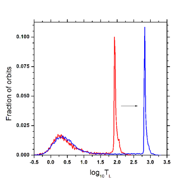
Figure 1: The histograms of circumbinary orbits in the Kepler-16 system in the Lyapunov time logarithm. The histogram of the orbits computed on the time interval of $10^{3}$ yr is shown in red, and that computed on the time interval of $10^{4}$ yr is shown in blue.

a)

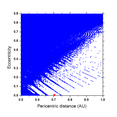
b)

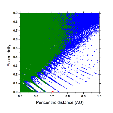
Figure 2: The stability diagrams constructed by the Lyapunov exponent criterion (a) and by the Lyapunov exponent plus escape-collision criteria (b). The regular regions are shown in white, chaotic in blue, and those for orbits with escapes and collisions (at the adopted time interval) in green. The location of the Kepler-16b planet is shown by a dot.

a)

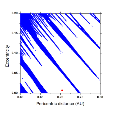
b)

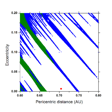
Figure 3: Zooms of the stability diagrams in Fig. 2, in a higher resolution.

a)

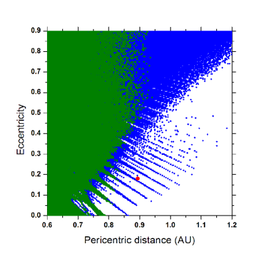
b)

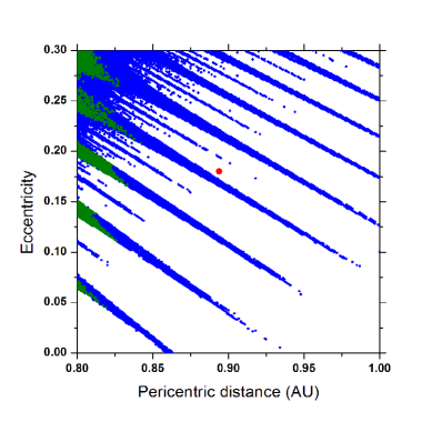
Figure 4: The same as in Figs. 2b and 3b, but for Kepler-34b.

a)

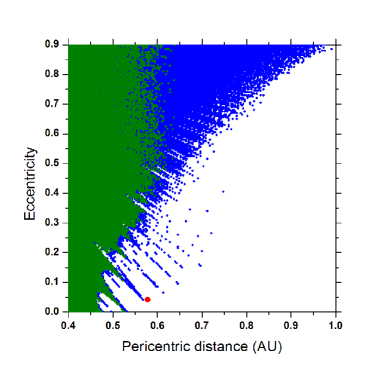
b)

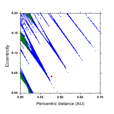
Figure 5: The same as in Figs. 2b and 3b, but for Kepler-35b.

References

- Chirikov (1959) Chirikov, B.V. 1959, Atomnaya Energiya, 6, 630 [1960, J. Nucl. Energy Part C: Plasma Phys., 1, 253]
- Chirikov (1979) Chirikov, B.V. 1979, Phys. Rep., 52, 263
- Deller & Maddison (2005) Deller, A.T., & Maddison, S.T. 2005, Astrophys. J., 625, 398
- Doyle et al. (2011) Doyle, L. et al., 2011, Science, 333, 1602
- Duncan et al. (1989) Duncan, M., Quinn, T., & Tremaine, S. 1989, Icarus, 82, 402
- Gladman et al. (2012) Gladman, B. et al., 2012, Astron. J., 144, 23
- Hairer et al. (1987) Hairer, E., Nørsett, S.P., & Wanner, G. 1987, Solving Ordinary Differential Equations I. Nonstiff Problems (New York: Springer)
- Holman & Murray (1996) Holman, M.J., & Murray, N.W. 1996, Astron. J., 112, 1278
- Holman & Wiegert (1999) Holman, M.J., & Wiegert, P.A. 1999, Astron. J., 117, 621
- Kouprianov & Shevchenko (2003) Kouprianov, V.V., & Shevchenko, I.I. 2003, Astron. Astrophys., 410, 749
- Kouprianov & Shevchenko (2005) Kouprianov, V.V., & Shevchenko, I.I. 2005, Icarus, 176, 224
- Lichtenberg & Lieberman (1992) Lichtenberg, A.J., & Lieberman, M.A. 1992, Regular and Chaotic Dynamics (New York: Springer)
- Melnikov & Shevchenko (1998) Melnikov, A.V., & Shevchenko, I.I. 1998, Sol. Sys. Res., 32, 480 (Astron. Vestnik, 32, 548)
- Melnikov & Shevchenko (2010) Melnikov, A.V., & Shevchenko, I.I. 2010, Icarus, 209, 786
- Meschiari (2012) Meschiari, S. 2012, Astrophys. J., 752, 71
- Morbidelli (2002) Morbidelli, A. 2002, Modern Celestial Mechanics (Taylor and Francis, Padstow)
- Moriwaki & Nakagawa (2004) Moriwaki, K., & Nakagawa, Y. 2004, Astrophys. J., 609, 1065
- Mudryk & Wu (2006) Mudryk, L.R., & Wu, Y. 2006, Astrophys. J., 639, 423
- Murray & Dermott (1999) Murray, C.D., & Dermott, S.F. 1999, Solar System Dynamics (Cambridge: Cambridge Univ. Press)
- Murray & Holman (1997) Murray, N.W., & Holman, M.J. 1997, Astron. J., 114, 1246
- Orosz et al. (2012a) Orosz, J.A. et al., 2012, Astrophys. J., 758, 87
- Orosz et al. (2012b) Orosz, J.A. et al., 2012, Science, 337, 1511
- Paardekooper et al. (2012) Paardekooper, S.-J., Leinhardt, Z.M., Thébault, T., Baruteau, C. 2012, Astrophys. J., 754, L16
- Pierens & Nelson (2007) Pierens, A., & Nelson, R.P. 2007, Astron. Astrophys., 472, 993
- Pierens & Nelson (2008) Pierens, A., & Nelson, R.P. 2008, Astron. Astrophys., 483, 633
- Quillen (2006) Quillen, A.C. 2006, MNRAS, 365, 1367
- Popova & Shevchenko (2012) Popova, E.A., & Shevchenko, I.I. 2012, Astron. Lett., 38, 581 (Pis’ma Astron. Zhurnal, 38, 652)
- Shevchenko (2002) Shevchenko, I.I. 2002, in Asteroids, Comets, Meteors 2002, ed. by Warmbein, B. (Berlin: ESA) 367
- Shevchenko & Kouprianov (2002) Shevchenko, I.I., & Kouprianov, V.V. 2002, Astron. Astrophys., 394, 663
- Shevchenko & Melnikov (2003) Shevchenko, I.I., & Melnikov, A.V. 2003, JETP Lett., 77, 642 (Pis’ma ZhETF, 77, 772)
- von Bremen et al. (1997) von Bremen, H.F., Udwadia, F.E., & Proskurowski, W. 1997, Physica D, 101, 1
- Welsh et al. (2012) Welsh, W.F. et al., 2012, Nature, 481, 475
- Wisdom (1980) Wisdom, J. 1980, Astron. J., 85, 1122
- Wisdom (1987) Wisdom, J. 1987, Astron. J., 94, 1350
a)