Density-Difference Estimation

Abstract

We address the problem of estimating the difference between two probability densities. A naive approach is a two-step procedure of first estimating two densities separately and then computing their difference. However, such a two-step procedure does not necessarily work well because the first step is performed without regard to the second step and thus a small error incurred in the first stage can cause a big error in the second stage. In this paper, we propose a single-shot procedure for directly estimating the density difference without separately estimating two densities. We derive a non-parametric finite-sample error bound for the proposed single-shot density-difference estimator and show that it achieves the optimal convergence rate. The usefulness of the proposed method is also demonstrated experimentally.

Keywords

density difference, $L^{2}$-distance, robustness, Kullback-Leibler divergence, kernel density estimation.

1 Introduction

When estimating a quantity consisting of two elements, a two-stage approach of first estimating the two elements separately and then approximating the target quantity based on the estimates of the two elements often performs poorly, because the first stage is carried out without regard to the second stage and thus a small error incurred in the first stage can cause a big error in the second stage. To cope with this problem, it would be more appropriate to directly estimate the target quantity in a single-shot process without separately estimating the two elements.

A seminal example that follows this general idea is pattern recognition by the support vector machine [COLT:Boser+etal:1992, mach:Cortes+Vapnik:1995, book:Vapnik:1998]: Instead of separately estimating two probability distributions of patterns for positive and negative classes, the support vector machine directly learns the boundary between the two classes that is sufficient for pattern recognition. More recently, a problem of estimating the ratio of two probability densities was tackled in a similar fashion [Biometrika:Qin:1998, AISM:Sugiyama+etal:2008, Inbook:Gretton+etal:2009, JMLR:Kanamori+etal:2009, IEEE-IT:Nguyen+etal:2010, ML:Kanamori+etal:2012, AISM:Sugiyama+etal:2012, book:Sugiyama+etal:2012]: The ratio of two probability densities is directly estimated without going through separate estimation of the two probability densities.

In this paper, we further explore this line of research, and propose a method for directly estimating the difference between two probability densities in a single-shot process. Density differences are useful for various purposes such as class-balance estimation under class-prior change [nc:Saerens+Latinne+Decaestecker:2002, ICML:duPlessis+Sugiyama:2012], change-point detection in time series [SAM:Kawahara+Sugiyama:2012, arXiv:Song+etal:2012], feature extraction [JMLR:Torkkola:2003], video-based event detection [VECTaR:Yamanaka+etal:2011], flow cytometric data analysis [BJ:Duong+etal:2009], ultrasound image segmentation [PR:Liu+eta:2010], non-rigid image registration [ANBC:Atif+etal:2003], and image-based target recognition [SPIE:Gray+Principe:2010].

For this density-difference estimation problem, we propose a single-shot method, called the least-squares density-difference (LSDD) estimator, that directly estimates the density difference without separately estimating two densities. LSDD is derived within a framework of kernel least-squares estimation, and its solution can be computed analytically in a computationally efficient and stable manner. Furthermore, LSDD is equipped with cross-validation, and thus all tuning parameters such as the kernel width and the regularization parameter can be systematically and objectively optimized. We derive a finite-sample error bound for the LSDD estimator in a non-parametric setup and show that it achieves the optimal convergence rate.

We also apply LSDD to $L^{2}$-distance estimation and show that it is more accurate than the difference of KDEs, which tends to severely under-estimate the $L^{2}$-distance [JMA:Anderson+etal:1994]. Compared with the Kullback-Leibler (KL) divergence [Annals-Math-Stat:Kullback+Leibler:1951], the $L^{2}$-distance is more robust against outliers [Biometrika:Basu+etal:1998, Tech:Scott:2001, CSDA:Besbeas+Morgan:2004].

Finally, we experimentally demonstrate the usefulness of LSDD in semi-supervised class-prior estimation and unsupervised change detection.

The rest of this paper is structured as follows. In Section 2, we derive the LSDD method and investigate its theoretical properties. In Section 3, we show how the $L^{2}$-distance can be approximated by LSDD. In Section 4, we illustrate the numerical behavior of LSDD. Finally, we conclude in Section 5.

2 Density-Difference Estimation

In this section, we propose a single-shot method for estimating the difference between two probability densities from samples, and analyze its theoretical properties.

2.1 Problem Formulation and Naive Approach

First, we formulate the problem of density-difference estimation.

Suppose that we are given two sets of independent and identically distributed samples ${\mathcal{X}}:=\{{\boldsymbol{x}}_{i}\}_{i=1}^{n}$ and ${\mathcal{X}}^{\prime}:=\{{\boldsymbol{x}}^{\prime}_{i^{\prime}}\}_{i^{\prime}=1}^{n^{\prime}}$ drawn from probability distributions on $\mathbb{R}^{d}$ with densities $p({\boldsymbol{x}})$ and $p^{\prime}({\boldsymbol{x}})$, respectively:

$${\mathcal{X}} :=\{{\boldsymbol{x}}_{i}\}_{i=1}^{n}\stackrel{{\scriptstyle\mathrm{i.i.d.}}}{{\sim}}p({\boldsymbol{x}}),$$

$${\mathcal{X}}^{\prime} :=\{{\boldsymbol{x}}^{\prime}_{i^{\prime}}\}_{i^{\prime}=1}^{n^{\prime}}\stackrel{{\scriptstyle\mathrm{i.i.d.}}}{{\sim}}p^{\prime}({\boldsymbol{x}}).$$

Our goal is to estimate the difference $f({\boldsymbol{x}})$ between $p({\boldsymbol{x}})$ and $p^{\prime}({\boldsymbol{x}})$ from the samples ${\mathcal{X}}$ and ${\mathcal{X}}^{\prime}$:

$$f({\boldsymbol{x}}):=p({\boldsymbol{x}})-p^{\prime}({\boldsymbol{x}}).$$

A naive approach to density-difference estimation is to use kernel density estimators (KDEs) [book:Silverman:1986]. For Gaussian kernels, the KDE-based density-difference estimator is given by

$$\widetilde{f}({\boldsymbol{x}}):=\widehat{p}({\boldsymbol{x}})-\widehat{p}^{\prime}({\boldsymbol{x}}),$$

where

$$\widehat{p}({\boldsymbol{x}}) :=\frac{1}{n(2\pi\sigma^{2})^{d/2}}\sum_{i=1}^{n}\exp\left(-\frac{\|{\boldsymbol{x}}-{\boldsymbol{x}}_{i}\|^{2}}{2\sigma^{2}}\right),$$

$$\widehat{p}^{\prime}({\boldsymbol{x}}) :=\frac{1}{n^{\prime}(2\pi\sigma^{\prime 2})^{d/2}}\sum_{i^{\prime}=1}^{n^{\prime}}\exp\left(-\frac{\|{\boldsymbol{x}}-{\boldsymbol{x}}^{\prime}_{i^{\prime}}\|^{2}}{2\sigma^{\prime 2}}\right).$$

The Gaussian widths $\sigma$ and $\sigma^{\prime}$ may be determined based on cross-validation [book:Haerdle+etal:2004].

However, we argue that the KDE-based density-difference estimator is not the best approach because of its two-step nature: Small estimation error in each density estimate can cause a big error in the final density-difference estimate. More intuitively, good density estimators tend to be smooth and thus a density-difference estimator obtained from such smooth density estimators tends to be over-smoothed [Biometrika:Hall+Wand:1988, JMA:Anderson+etal:1994, see also numerical experiments in Section 4.1.1].

To overcome this weakness, we give a single-shot procedure of directly estimating the density difference $f({\boldsymbol{x}})$ without separately estimating the densities $p({\boldsymbol{x}})$ and $p^{\prime}({\boldsymbol{x}})$.

2.2 Least-Squares Density-Difference Estimation

In our proposed approach, we fit a density-difference model $g({\boldsymbol{x}})$ to the true density-difference function $f({\boldsymbol{x}})$ under the squared loss:

$$\mathop{\mathrm{argmin\,}}_{g}\int\left(g({\boldsymbol{x}})-f({\boldsymbol{x}})\right)^{2}\mathrm{d}{\boldsymbol{x}}.$$ (1)

We use the following linear-in-parameter model as $g({\boldsymbol{x}})$:

$$g({\boldsymbol{x}})=\sum_{\ell=1}^{b}\theta_{\ell}\psi_{\ell}({\boldsymbol{x}})={\boldsymbol{\theta}}^{\top}{\boldsymbol{\psi}}({\boldsymbol{x}}),$$ (2)

where $b$ denotes the number of basis functions, ${\boldsymbol{\psi}}({\boldsymbol{x}})=(\psi_{1}({\boldsymbol{x}}),\ldots,\psi_{b}({\boldsymbol{x}}))^{\top}$ is a $b$-dimensional basis function vector, ${\boldsymbol{\theta}}=(\theta_{1},\ldots,\theta_{b})^{\top}$ is a $b$-dimensional parameter vector, and ^⊤ denotes the transpose. In practice, we use the following non-parametric Gaussian kernel model as $g({\boldsymbol{x}})$:

$$g({\boldsymbol{x}})=\sum_{\ell=1}^{n+n^{\prime}}\theta_{\ell}\exp\left(-\frac{\|{\boldsymbol{x}}-{\boldsymbol{c}}_{\ell}\|^{2}}{2\sigma^{2}}\right),$$ (3)

where $({\boldsymbol{c}}_{1},\ldots,{\boldsymbol{c}}_{n},{\boldsymbol{c}}_{n+1},\ldots,{\boldsymbol{c}}_{n+n^{\prime}}):=({\boldsymbol{x}}_{1},\ldots,{\boldsymbol{x}}_{n},{\boldsymbol{x}}^{\prime}_{1},\ldots,{\boldsymbol{x}}^{\prime}_{n^{\prime}})$ are Gaussian kernel centers. If $n+n^{\prime}$ is large, we may use only a subset of ${\boldsymbol{x}}_{1},\ldots,{\boldsymbol{x}}_{n},{\boldsymbol{x}}^{\prime}_{1},\ldots,{\boldsymbol{x}}^{\prime}_{n^{\prime}}$ as Gaussian kernel centers.

For the model (2), the optimal parameter ${\boldsymbol{\theta}}^{\ast}$ is given by

$${\boldsymbol{\theta}}^{\ast} :=\mathop{\mathrm{argmin\,}}_{{\boldsymbol{\theta}}}\int\left(g({\boldsymbol{x}})-f({\boldsymbol{x}})\right)^{2}\mathrm{d}{\boldsymbol{x}}$$

$$\phantom{:}=\mathop{\mathrm{argmin\,}}_{{\boldsymbol{\theta}}}\left[\int g({\boldsymbol{x}})^{2}\mathrm{d}{\boldsymbol{x}}-2\int g({\boldsymbol{x}})f({\boldsymbol{x}})\mathrm{d}{\boldsymbol{x}}\right]$$

$$\phantom{:}=\mathop{\mathrm{argmin\,}}_{{\boldsymbol{\theta}}}\left[{\boldsymbol{\theta}}^{\top}{\boldsymbol{H}}{\boldsymbol{\theta}}-2{\boldsymbol{h}}^{\top}{\boldsymbol{\theta}}\right]$$

$$\phantom{:}={\boldsymbol{H}}^{-1}{\boldsymbol{h}},$$

where ${\boldsymbol{H}}$ is the $b\times b$ matrix and ${\boldsymbol{h}}$ is the $b$-dimensional vector defined as

$${\boldsymbol{H}} :=\int{\boldsymbol{\psi}}({\boldsymbol{x}}){\boldsymbol{\psi}}({\boldsymbol{x}})^{\top}\mathrm{d}{\boldsymbol{x}},$$

$${\boldsymbol{h}} :=\int{\boldsymbol{\psi}}({\boldsymbol{x}})p({\boldsymbol{x}})\mathrm{d}{\boldsymbol{x}}-\int{\boldsymbol{\psi}}({\boldsymbol{x}}^{\prime})p^{\prime}({\boldsymbol{x}}^{\prime})\mathrm{d}{\boldsymbol{x}}^{\prime}.$$

Note that, for the Gaussian kernel model (3), the integral in ${\boldsymbol{H}}$ can be computed analytically as

$$H_{\ell,\ell^{\prime}} =\int\exp\left(-\frac{\|{\boldsymbol{x}}-{\boldsymbol{c}}_{\ell}\|^{2}}{2\sigma^{2}}\right)\exp\left(-\frac{\|{\boldsymbol{x}}-{\boldsymbol{c}}_{\ell^{\prime}}\|^{2}}{2\sigma^{2}}\right)\mathrm{d}{\boldsymbol{x}}$$

$$=(\pi\sigma^{2})^{d/2}\exp\left(-\frac{\|{\boldsymbol{c}}_{\ell}-{\boldsymbol{c}}_{\ell^{\prime}}\|^{2}}{4\sigma^{2}}\right),$$

where $d$ denotes the dimensionality of ${\boldsymbol{x}}$.

Replacing the expectations in ${\boldsymbol{h}}$ by empirical estimators and adding an $\ell_{2}$-regularizer to the objective function, we arrive at the following optimization problem:

$${\widehat{{\boldsymbol{\theta}}}}:=\mathop{\mathrm{argmin\,}}_{{\boldsymbol{\theta}}}\left[{\boldsymbol{\theta}}^{\top}{\boldsymbol{H}}{\boldsymbol{\theta}}-2{\widehat{{\boldsymbol{h}}}}^{\top}{\boldsymbol{\theta}}+\lambda{\boldsymbol{\theta}}^{\top}{\boldsymbol{\theta}}\right],$$ (4)

where $\lambda$ ($\geq 0$) is the regularization parameter and ${\widehat{{\boldsymbol{h}}}}$ is the $b$-dimensional vector defined as

$${\widehat{{\boldsymbol{h}}}} =\frac{1}{n}\sum_{i=1}^{n}{\boldsymbol{\psi}}({\boldsymbol{x}}_{i})-\frac{1}{n^{\prime}}\sum_{i^{\prime}=1}^{n^{\prime}}{\boldsymbol{\psi}}({\boldsymbol{x}}^{\prime}_{i^{\prime}}).$$

Taking the derivative of the objective function in Eq.(4) and equating it to zero, we can obtain the solution ${\widehat{{\boldsymbol{\theta}}}}$ analytically as

$${\widehat{{\boldsymbol{\theta}}}}=\left({\boldsymbol{H}}+\lambda{\boldsymbol{I}}_{b}\right)^{-1}{\widehat{{\boldsymbol{h}}}},$$

where ${\boldsymbol{I}}_{b}$ denotes the $b$-dimensional identity matrix.

Finally, a density-difference estimator $\widehat{f}({\boldsymbol{x}})$ is given as

$$\widehat{f}({\boldsymbol{x}})={\widehat{{\boldsymbol{\theta}}}}^{\top}{\boldsymbol{\psi}}({\boldsymbol{x}}).$$ (5)

We call this the least-squares density-difference (LSDD) estimator.

2.3 Theoretical Analysis

Here, we theoretically investigate the behavior of the LSDD estimator.

2.3.1 Parametric Convergence

First, we consider a linear parametric setup where basis functions in our density-difference model (2) are fixed.

Suppose that $n/(n+n^{\prime})$ converges to $\eta\in[0,1]$. Then the central limit theorem [book:Rao:1965] asserts that $\sqrt{\frac{nn^{\prime}}{n+n^{\prime}}}({\widehat{{\boldsymbol{\theta}}}}-{\boldsymbol{\theta}}^{\ast})$ converges in law to the normal distribution with mean ${\boldsymbol{0}}$ and covariance matrix

$${\boldsymbol{H}}^{-1}((1-\eta){\boldsymbol{V}}_{p}+\eta{\boldsymbol{V}}_{p^{\prime}}){\boldsymbol{H}}^{-1},$$

where ${\boldsymbol{V}}_{p}$ denotes the covariance matrix of ${\boldsymbol{\psi}}({\boldsymbol{x}})$ under the probability density $p({\boldsymbol{x}})$:

$${\boldsymbol{V}}_{p}:=\int\left({\boldsymbol{\psi}}({\boldsymbol{x}})-{\boldsymbol{\psi}}_{p}\right)\left({\boldsymbol{\psi}}({\boldsymbol{x}})-{\boldsymbol{\psi}}_{p}\right)^{\top}p({\boldsymbol{x}})\mathrm{d}{\boldsymbol{x}},$$ (6)

and ${\boldsymbol{\psi}}_{p}$ denotes the expectation of ${\boldsymbol{\psi}}({\boldsymbol{x}})$ under the probability density $p({\boldsymbol{x}})$:

$${\boldsymbol{\psi}}_{p}:=\int{\boldsymbol{\psi}}({\boldsymbol{x}})p({\boldsymbol{x}})\mathrm{d}{\boldsymbol{x}}.$$

This result implies that the LSDD estimator has asymptotic normality with asymptotic order $\sqrt{1/n+1/n^{\prime}}$, which is the optimal convergence rate in the parametric setup.

2.3.2 Non-Parametric Error Bound

Next, we consider a non-parametric setup where a density-difference function is learned in a Gaussian reproducing kernel Hilbert space (RKHS) [AMS:Aronszajn:1950].

Let $\mathcal{H}_{\gamma}$ be the Gaussian RKHS with width $\gamma$:

$$k_{\gamma}({\boldsymbol{x}},{\boldsymbol{x}}^{\prime})=\exp\left(-\frac{\|{\boldsymbol{x}}-{\boldsymbol{x}}^{\prime}\|^{2}}{\gamma^{2}}\right).$$

Let us consider a slightly modified LSDD estimator that is more suitable for non-parametric error analysis: For $n^{\prime}=n$,

$$\widehat{f}:=\mathop{\arg\min}_{g\in\mathcal{H}_{\gamma}}\left[\|g\|_{L^{2}}^{2}-2\left(\frac{1}{n}\sum_{i=1}^{n}g({\boldsymbol{x}}_{i})+\frac{1}{n}\sum_{i^{\prime}=1}^{n}g({\boldsymbol{x}}^{\prime}_{i^{\prime}})\right)+\lambda\|g\|^{2}_{\mathcal{H}_{\gamma}}\right],$$

where $\|\cdot\|_{L^{2}}$ denotes the $L^{2}$-norm and $\|\cdot\|_{\mathcal{H}_{\gamma}}$ denotes the norm in RKHS $\mathcal{H}_{\gamma}$.

Then we can prove that, for all $\rho,\rho^{\prime}>0$, there exists a constant $K$ such that, for all $\tau\geq 1$ and $n\geq 1$, the non-parametric LSDD estimator with appropriate choice of $\lambda$ and $\gamma$ satisfies

$$\|\widehat{f}-f\|_{L^{2}}^{2}+\lambda\|\widehat{f}\|_{\mathcal{H}_{\gamma}}^{2}\leq K\left(n^{-\frac{2\alpha}{2\alpha+d}+\rho}+\tau n^{-1+\rho^{\prime}}\right),$$ (7)

with probability not less than $1-4e^{-\tau}$. Here, $d$ denotes the dimensionality of input vector ${\boldsymbol{x}}$, and $\alpha\geq 0$ denotes the regularity of Besov space to which the true density-difference function $f$ belongs (smaller/larger $\alpha$ means $f$ is “less/more complex”; see Appendix A for its precise definition). Because $n^{-\frac{2\alpha}{2\alpha+d}}$ is the optimal learning rate in this setup [NIPS2011_0874], the above result shows that the non-parametric LSDD estimator achieves the optimal convergence rate.

It is known that, if the naive KDE with a Gaussian kernel is used for estimating a probability density with regularity $\alpha>2$, the optimal learning rate cannot be achieved [AMS:Farrell:1972, book:Silverman:1986]. To achieve the optimal rate by KDE, we should choose a kernel specifically tailored to each regularity $\alpha$ [AMS:Parzen:1962]. But such a kernel is not non-negative and it is difficult to implement in practice. On the other hand, our LSDD estimator can always achieve the optimal learning rate with a Gaussian kernel without regard to regularity $\alpha$.

2.4 Model Selection by Cross-Validation

The above theoretical analyses showed the superiority of LSDD. However, the practical performance of LSDD depends on the choice of models (i.e., the kernel width $\sigma$ and the regularization parameter $\lambda$). Here, we show that the model can be optimized by cross-validation (CV).

More specifically, we first divide the samples ${\mathcal{X}}=\{{\boldsymbol{x}}_{i}\}_{i=1}^{n}$ and ${\mathcal{X}}^{\prime}=\{{\boldsymbol{x}}^{\prime}_{i^{\prime}}\}_{i^{\prime}=1}^{n^{\prime}}$ into $T$ disjoint subsets $\{{\mathcal{X}}_{t}\}_{t=1}^{T}$ and $\{{\mathcal{X}}^{\prime}_{t}\}_{t=1}^{T}$, respectively. Then we obtain a density-difference estimate $\widehat{f}_{t}({\boldsymbol{x}})$ from ${\mathcal{X}}\backslash{\mathcal{X}}_{t}$ and ${\mathcal{X}}^{\prime}\backslash{\mathcal{X}}^{\prime}_{t}$ (i.e., all samples without ${\mathcal{X}}_{t}$ and ${\mathcal{X}}^{\prime}_{t}$), and compute its hold-out error for ${\mathcal{X}}_{t}$ and ${\mathcal{X}}^{\prime}_{t}$ as

$$\mathrm{CV}^{(t)} :=\int\!\widehat{f}_{t}({\boldsymbol{x}})^{2}\mathrm{d}{\boldsymbol{x}}-\frac{2}{|{\mathcal{X}}_{t}|}\!\sum_{{\boldsymbol{x}}\in{\mathcal{X}}_{t}}\!\!\widehat{f}_{t}({\boldsymbol{x}})+\frac{2}{|{\mathcal{X}}^{\prime}_{t}|}\!\sum_{{\boldsymbol{x}}^{\prime}\in{\mathcal{X}}^{\prime}_{t}}\!\!\widehat{f}_{t}({\boldsymbol{x}}^{\prime}),$$

where $|{\mathcal{X}}|$ denotes the number of elements in the set ${\mathcal{X}}$. We repeat this hold-out validation procedure for $t=1,\ldots,T$, and compute the average hold-out error as

$$\mathrm{CV} :=\frac{1}{T}\sum_{t=1}^{T}\mathrm{CV}^{(t)}.$$

Finally, we choose the model that minimizes $\mathrm{CV}$.

A MATLAB${}^{\text{\textregistered}}$ implementation of LSDD is available from

http://sugiyama-www.cs.titech.ac.jp/~sugi/software/LSDD/’.

(to be made public after acceptance)

3 $L^{2}$-Distance Estimation by LSDD

In this section, we consider the problem of approximating the $L^{2}$-distance between $p({\boldsymbol{x}})$ and $p^{\prime}({\boldsymbol{x}})$,

$$L^{2}(p,p^{\prime}):=\int\left(p({\boldsymbol{x}})-p^{\prime}({\boldsymbol{x}})\right)^{2}\mathrm{d}{\boldsymbol{x}},$$ (8)

from samples ${\mathcal{X}}:=\{{\boldsymbol{x}}_{i}\}_{i=1}^{n}$ and ${\mathcal{X}}^{\prime}:=\{{\boldsymbol{x}}^{\prime}_{i^{\prime}}\}_{i^{\prime}=1}^{n^{\prime}}$ (see Section 2.1).

3.1 Basic Form

For an equivalent expression

$$L^{2}(p,p^{\prime}) =\int f({\boldsymbol{x}})p({\boldsymbol{x}})\mathrm{d}{\boldsymbol{x}}-\int f({\boldsymbol{x}}^{\prime})p^{\prime}({\boldsymbol{x}}^{\prime})\mathrm{d}{\boldsymbol{x}}^{\prime},$$

if we replace $f({\boldsymbol{x}})$ with an LSDD estimator $\widehat{f}({\boldsymbol{x}})$ and approximate the expectations by empirical averages, the following $L^{2}$-distance estimator can be obtained:

$$L^{2}(p,p^{\prime})\approx{\widehat{{\boldsymbol{h}}}}^{\top}{\widehat{{\boldsymbol{\theta}}}}.$$ (9)

Similarly, for another expression

$$L^{2}(p,p^{\prime}) =\int f({\boldsymbol{x}})^{2}\mathrm{d}{\boldsymbol{x}},$$

replacing $f({\boldsymbol{x}})$ with an LSDD estimator $\widehat{f}({\boldsymbol{x}})$ gives another $L^{2}$-distance estimator:

$$L^{2}(p,p^{\prime})\approx{\widehat{{\boldsymbol{\theta}}}}^{\top}{\boldsymbol{H}}{\widehat{{\boldsymbol{\theta}}}}.$$ (10)

3.2 Reduction of Bias Caused by Regularization

Eq.(9) and Eq.(10) themselves give approximations to $L^{2}(p,p^{\prime})$. Nevertheless, we argue that the use of their combination, defined by

$$\widehat{L}^{2}({\mathcal{X}},{\mathcal{X}}^{\prime}):=2{\widehat{{\boldsymbol{h}}}}^{\top}{\widehat{{\boldsymbol{\theta}}}}-{\widehat{{\boldsymbol{\theta}}}}^{\top}{\boldsymbol{H}}{\widehat{{\boldsymbol{\theta}}}},$$ (11)

is more sensible. To explain the reason, let us consider a generalized $L^{2}$-distance estimator of the following form:

$$\beta{\widehat{{\boldsymbol{h}}}}^{\top}{\widehat{{\boldsymbol{\theta}}}}+(1-\beta){\widehat{{\boldsymbol{\theta}}}}^{\top}{\boldsymbol{H}}{\widehat{{\boldsymbol{\theta}}}},$$ (12)

where $\beta$ is a real scalar. If the regularization parameter $\lambda$ ($\geq 0$) is small, then Eq.(12) can be expressed as

$$\beta{\widehat{{\boldsymbol{h}}}}^{\top}{\widehat{{\boldsymbol{\theta}}}}+(1-\beta){\widehat{{\boldsymbol{\theta}}}}^{\top}{\boldsymbol{H}}{\widehat{{\boldsymbol{\theta}}}}={\widehat{{\boldsymbol{h}}}}^{\top}{\boldsymbol{H}}^{-1}{\widehat{{\boldsymbol{h}}}}-\lambda(2-\beta){\widehat{{\boldsymbol{h}}}}^{\top}{\boldsymbol{H}}^{-2}{\widehat{{\boldsymbol{h}}}}+o_{p}(\lambda),$$ (13)

where $o_{p}$ denotes the probabilistic order (its derivation is given in Appendix B).

Thus, the bias introduced by regularization (i.e., the second term in the right-hand side of Eq.(13) that depends on $\lambda$) can be eliminated if $\beta=2$, which yields Eq.(11). Note that, if no regularization is imposed (i.e., $\lambda=0$), both Eq.(9) and Eq.(10) yield ${\widehat{{\boldsymbol{h}}}}^{\top}{\boldsymbol{H}}^{-1}{\widehat{{\boldsymbol{h}}}}$, the first term in the right-hand side of Eq.(13).

Eq.(11) is actually equivalent to the negative of the optimal objective value of the LSDD optimization problem without regularization (i.e., Eq.(4) with $\lambda=0$). This can be naturally interpreted through a lower bound of $L^{2}(p,p^{\prime})$ obtained by Legendre-Fenchel convex duality [book:Rockafellar:1970]:

$$L^{2}(p,p^{\prime})=\sup_{g}\left[2\left(\int g({\boldsymbol{x}})p({\boldsymbol{x}})\mathrm{d}{\boldsymbol{x}}-\int g({\boldsymbol{x}})p^{\prime}({\boldsymbol{x}})\mathrm{d}{\boldsymbol{x}}\right)-\int g({\boldsymbol{x}})^{2}\mathrm{d}{\boldsymbol{x}}\right],$$

where the supremum is attained at $g=f$. If the expectations are replaced by empirical estimators and the linear-in-parameter model (2) is used as $g$, the above optimization problem is reduced to the LSDD objective function without regularization (see Eq.(4)). Thus, LSDD corresponds to approximately maximizing the above lower bound and Eq.(11) is its maximum value.

Through eigenvalue decomposition of ${\boldsymbol{H}}$, we can show that

$$2{\widehat{{\boldsymbol{h}}}}^{\top}{\widehat{{\boldsymbol{\theta}}}}-{\widehat{{\boldsymbol{\theta}}}}^{\top}{\boldsymbol{H}}{\widehat{{\boldsymbol{\theta}}}}\geq{\widehat{{\boldsymbol{h}}}}^{\top}{\widehat{{\boldsymbol{\theta}}}}\geq{\widehat{{\boldsymbol{\theta}}}}^{\top}{\boldsymbol{H}}{\widehat{{\boldsymbol{\theta}}}}.$$

Thus, our approximator (11) is not less than the plain approximators (9) and (10).

3.3 Further Bias Correction

${\widehat{{\boldsymbol{h}}}}^{\top}{\boldsymbol{H}}^{-1}{\widehat{{\boldsymbol{h}}}}$, the first term in Eq.(13), is an essential part of the $L^{2}$-distance estimator (11). However, it is actually a slightly biased estimator of the target quantity ${\boldsymbol{h}}^{\top}{\boldsymbol{H}}^{-1}{\boldsymbol{h}}$ ($={\boldsymbol{\theta}}^{*}{}^{\top}{\boldsymbol{H}}{\boldsymbol{\theta}}^{*}={\boldsymbol{h}}^{\top}{\boldsymbol{\theta}}^{*}$):

$$\mathbb{E}[{\widehat{{\boldsymbol{h}}}}^{\top}{\boldsymbol{H}}^{-1}{\widehat{{\boldsymbol{h}}}}]={\boldsymbol{h}}^{\top}{\boldsymbol{H}}^{-1}{\boldsymbol{h}}+\mathrm{tr}\left({\boldsymbol{H}}^{-1}\left(\frac{1}{n}{\boldsymbol{V}}_{p}+\frac{1}{n^{\prime}}{\boldsymbol{V}}_{p^{\prime}}\right)\right),$$ (14)

where $\mathbb{E}$ denotes the expectation over all samples ${\mathcal{X}}=\{{\boldsymbol{x}}_{i}\}_{i=1}^{n}$ and ${\mathcal{X}}^{\prime}=\{{\boldsymbol{x}}^{\prime}_{i^{\prime}}\}_{i^{\prime}=1}^{n^{\prime}}$, and ${\boldsymbol{V}}_{p}$ and ${\boldsymbol{V}}_{p^{\prime}}$ are defined by Eq.(6) (its derivation is given in Appendix C).

The second term in the right-hand side of Eq.(14) is an estimation bias that is generally non-zero. Thus, based on Eq.(14), we can construct a bias-corrected $L^{2}$-distance estimator as

$$\widetilde{L}^{2}({\mathcal{X}},{\mathcal{X}}^{\prime}):=2{\widehat{{\boldsymbol{h}}}}^{\top}{\widehat{{\boldsymbol{\theta}}}}-{\widehat{{\boldsymbol{\theta}}}}^{\top}{\boldsymbol{H}}{\widehat{{\boldsymbol{\theta}}}}-\mathrm{tr}\left({\boldsymbol{H}}^{-1}\left(\frac{1}{n}\widehat{{\boldsymbol{V}}}_{p}+\frac{1}{n^{\prime}}\widehat{{\boldsymbol{V}}}_{p^{\prime}}\right)\right),$$ (15)

where $\widehat{{\boldsymbol{V}}}_{p}$ is an empirical estimator of covariance matrix ${\boldsymbol{V}}_{p}$:

$$\widehat{{\boldsymbol{V}}}_{p}:=\frac{1}{n}\sum_{i=1}^{n}\left({\boldsymbol{\psi}}({\boldsymbol{x}}_{i})-\widehat{{\boldsymbol{\psi}}}_{p}\right)\left({\boldsymbol{\psi}}({\boldsymbol{x}}_{i})-\widehat{{\boldsymbol{\psi}}}_{p}\right)^{\top},$$

and $\widehat{{\boldsymbol{\psi}}}_{p}$ is an empirical estimator of the expectation ${\boldsymbol{\psi}}_{p}$:

$$\widehat{{\boldsymbol{\psi}}}_{p}:=\frac{1}{n}\sum_{i=1}^{n}{\boldsymbol{\psi}}({\boldsymbol{x}}_{i}).$$

The true $L^{2}$-distance is non-negative by definition (see Eq.(8)), but the above bias-corrected estimate can take a negative value. Following the same line as ? (?), the positive-part estimator may be more accurate:

$$\overline{L}^{2}({\mathcal{X}},{\mathcal{X}}^{\prime}):=\max\left\{0,\widetilde{L}^{2}({\mathcal{X}},{\mathcal{X}}^{\prime})\right\}.$$

However, in our preliminary experiments, $\overline{L}^{2}({\mathcal{X}},{\mathcal{X}}^{\prime})$ does not always perform well particularly when ${\boldsymbol{H}}$ is ill-conditioned. For this reason, we practically propose to use $\widehat{L}^{2}({\mathcal{X}},{\mathcal{X}}^{\prime})$ defined by Eq.(11).

4 Experiments

In this section, we experimentally evaluate the performance of LSDD.

4.1 Numerical Examples

First, we show numerical examples using artificial datasets.

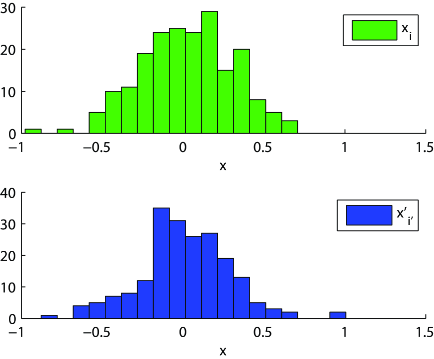
(a) Samples

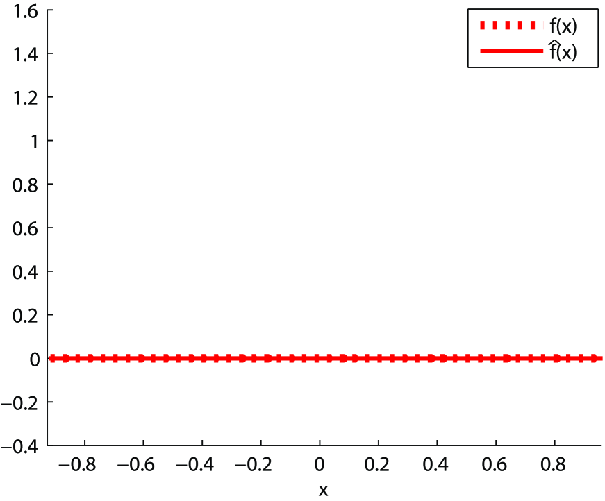
(b) LSDD

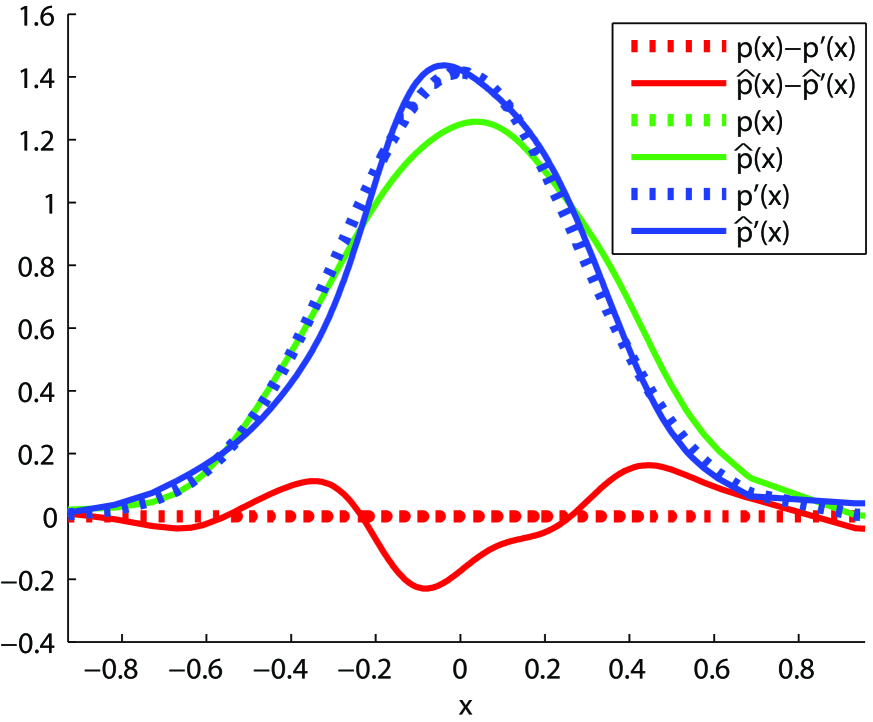
(c) KDE

Figure 1: Estimation of density difference when $\mu=0$ (i.e., $f(x)=p(x)-p^{\prime}(x)=0$).

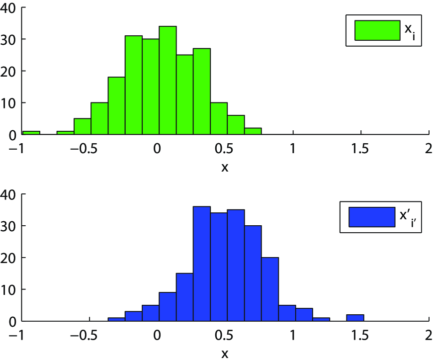
(a) Samples

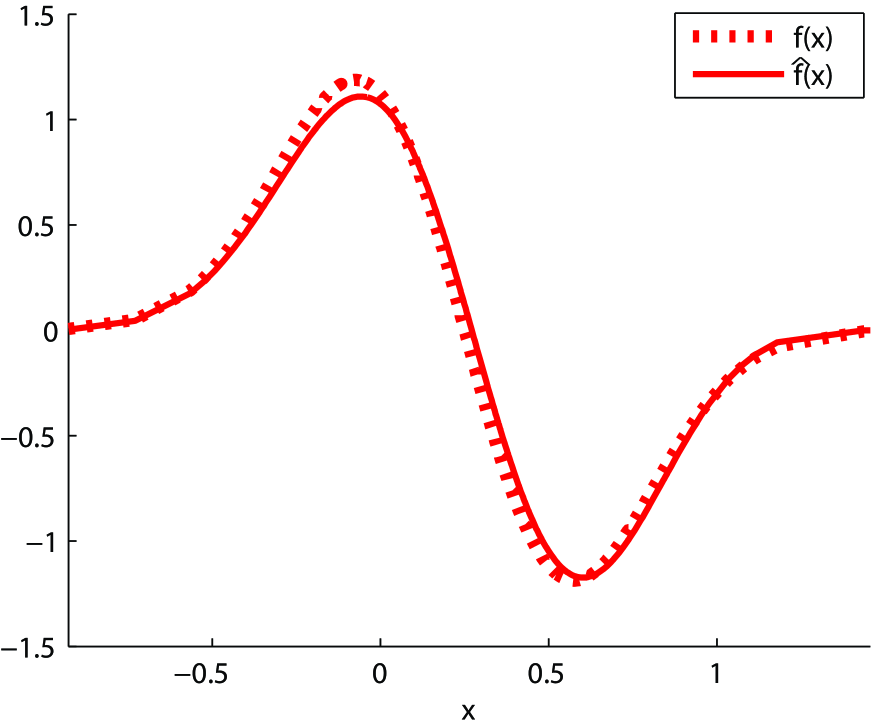
(b) LSDD

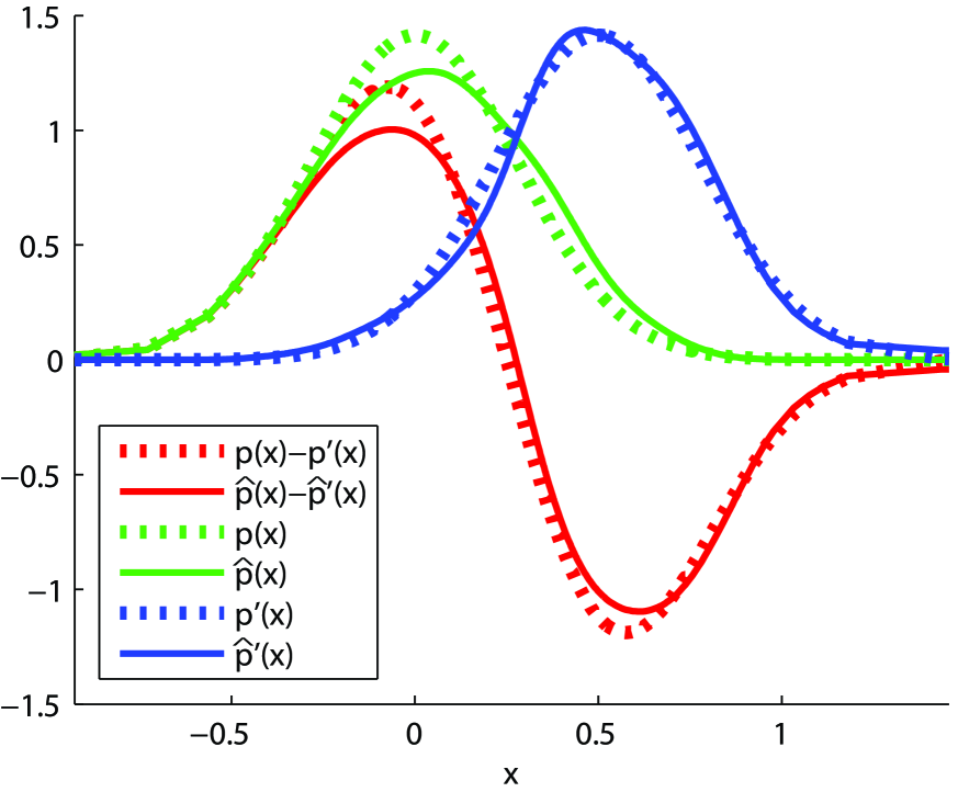
(c) KDE

Figure 2: Estimation of density difference when $\mu=0.5$ (i.e., $f(x)=p(x)-p^{\prime}(x)\neq 0$).

4.1.1 LSDD vs. KDE

We experimentally compare the behavior of LSDD and the KDE-based method. Let

$$p({\boldsymbol{x}}) =N({\boldsymbol{x}};(\mu,0,\ldots,0)^{\top},(4\pi)^{-1}{\boldsymbol{I}}_{d}),$$

$$p^{\prime}({\boldsymbol{x}}) =N({\boldsymbol{x}};(0,0,\ldots,0)^{\top},(4\pi)^{-1}{\boldsymbol{I}}_{d}),$$

where $N({\boldsymbol{x}};{\boldsymbol{\mu}},{\boldsymbol{\Sigma}})$ denotes the multi-dimensional normal density with mean vector ${\boldsymbol{\mu}}$ and variance-covariance matrix ${\boldsymbol{\Sigma}}$ with respect to ${\boldsymbol{x}}$, and ${\boldsymbol{I}}_{d}$ denotes the $d$-dimensional identity matrix.

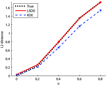
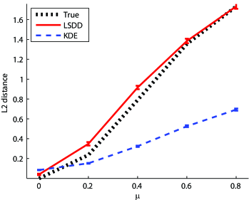
(a) $d=1$	(b) $d=5$

Figure 3: $L^{2}$-distance estimation by LSDD and KDE. Means and standard errors over $100$ runs are plotted.

We first illustrate how LSDD and KDE behave under $d=1$ and $n=n^{\prime}=200$. Figure 2 depicts the data samples, densities and density difference estimated by KDE, and density difference estimated by LSDD for $\mu=0$ (i.e., $f(x)=p(x)-p^{\prime}(x)=0$). This shows that LSDD gives a more accurate estimate of the density difference $f(x)$ than KDE. Figure 2 depicts the results for $\mu=0.5$ (i.e., $f(x)\neq 0$), showing again that LSDD performs well.

Next, we compare the $L^{2}$-distance approximator based on LSDD and that based on KDE. For $\mu=0,0.2,0.4,0.6,0.8$ and $d=1,5$, we draw $n=n^{\prime}=200$ samples from the above $p({\boldsymbol{x}})$ and $p^{\prime}({\boldsymbol{x}})$. Figure 3 depicts the mean and standard error of estimated $L^{2}$-distances over $100$ runs as functions of mean $\mu$. When $d=1$, the LSDD-based $L^{2}$-distance estimator gives accurate estimates of the true $L^{2}$-distance, whereas the KDE-based $L^{2}$-distance estimator slightly underestimates the true $L^{2}$-distance. This is caused by the fact that KDE tends to provide smoother density estimates (see Figure 2(c) again). Such smoother density estimates are accurate as density estimates, but the difference of smoother density estimates yields a smaller $L^{2}$-distance estimate [JMA:Anderson+etal:1994]. This tendency is more significant when $d=5$; the KDE-based $L^{2}$-distance estimator severely underestimates the true $L^{2}$-distance, which is a typical drawback of the two-step procedure. On the other hand, the LSDD-based $L^{2}$-distance estimator still gives reasonably accurate estimates of the true $L^{2}$-distance even when $d=5$.

4.1.2 $L^{2}$-Distance vs. KL-Divergence

The Kullback-Leibler (KL) divergence [Annals-Math-Stat:Kullback+Leibler:1951] is a popular divergence measure for comparing probability distributions. The KL-divergence from $p({\boldsymbol{x}})$ to $p^{\prime}({\boldsymbol{x}})$ is defined as

$$\mathrm{KL}(p\|p^{\prime}):=\int p({\boldsymbol{x}})\log\frac{p({\boldsymbol{x}})}{p^{\prime}({\boldsymbol{x}})}\mathrm{d}{\boldsymbol{x}}.$$

First, we illustrate the difference between the $L^{2}$-distance and the KL-divergence. For $d=1$, let

$$p(x) =(1-\eta)N(x;0,1^{2})+\eta N(x;\mu,1/4^{2}),$$

$$p^{\prime}(x) =N(x;0,1^{2}).$$

Implications of the above densities are that samples drawn from $N(x;0,1^{2})$ are inliers, whereas samples drawn from $N(x;\mu,1/4^{2})$ are outliers. We set the outlier rate at $\eta=0.1$ and the outlier mean at $\mu=0,2,4,\ldots,10$ (see Figure 8).

Figure 8 depicts the $L^{2}$-distance and the KL-divergence for outlier mean $\mu=0,2,4,\ldots,10$. This shows that both the $L^{2}$-distance and the KL-divergence increase as $\mu$ increases. However, the $L^{2}$-distance is bounded from above, whereas the KL-divergence diverges to infinity as $\mu$ tends to infinity. This result implies that the $L^{2}$-distance is less sensitive to outliers than the KL-divergence, which well agrees with the observation given in ? (?).

Next, we draw $n=n^{\prime}=100$ samples from $p(x)$ and $p^{\prime}(x)$, and estimate the $L^{2}$-distance by LSDD and the KL-divergence by the Kullback-Leibler importance estimation procedure (KLIEP) [AISM:Sugiyama+etal:2008, IEEE-IT:Nguyen+etal:2010]. Figure 8 depicts the estimated $L^{2}$-distance and KL-divergence for outlier mean $\mu=0,2,4,\ldots,10$ over $100$ runs. This shows that both LSDD and KLIEP reasonably capture the profiles of the true $L^{2}$-distance and the KL-divergence, although the scale of KLIEP values is much different from the true values (see Figure 8) because the estimated normalization factor was unreliable.

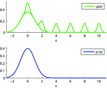
Figure 4: Comparing two densities in the presence of outliers. $p(x)$ includes outliers at $\mu=0,2,4,\ldots,10$.

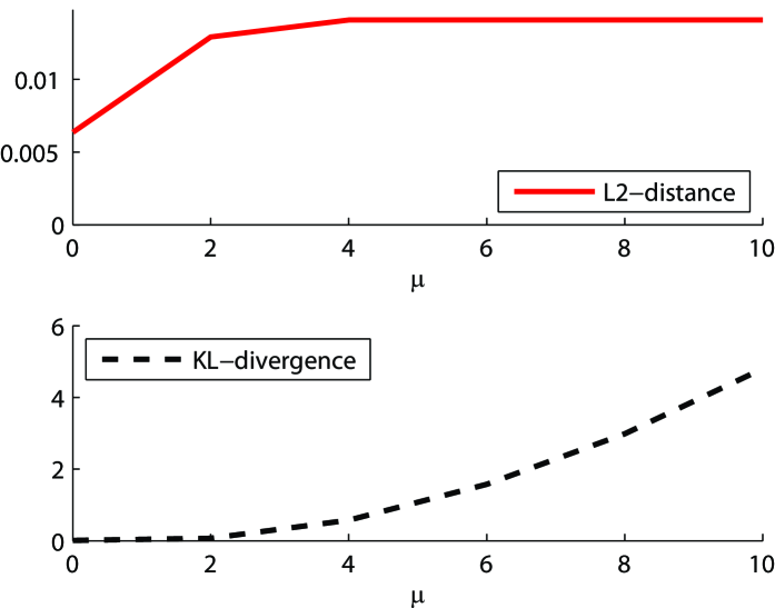
Figure 5: The true $L^{2}$-distance and true KL-divergence as functions of outlier mean $\mu$.

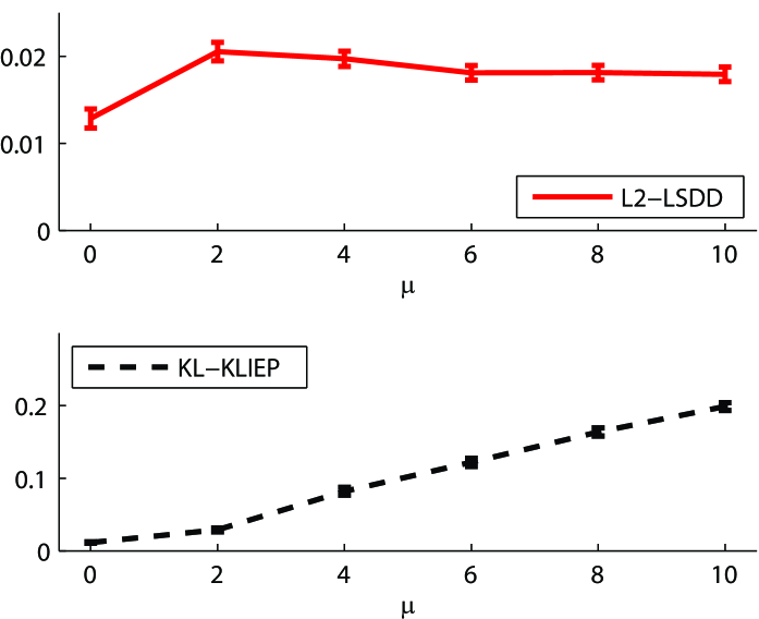
Figure 6: Means and standard errors of $L^{2}$-distance estimation by LSDD and KL-divergence estimation by KLIEP over $100$ runs.

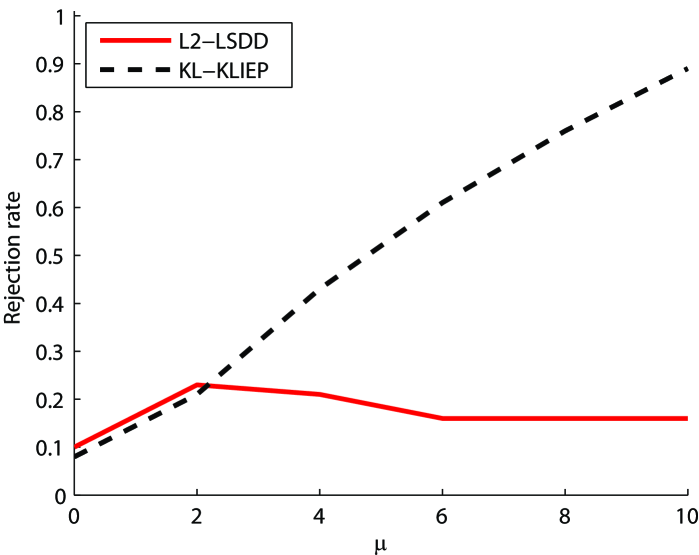
Figure 7: Two-sample test for outlier rate $\eta=0.1$ as functions of outlier mean $\mu$.

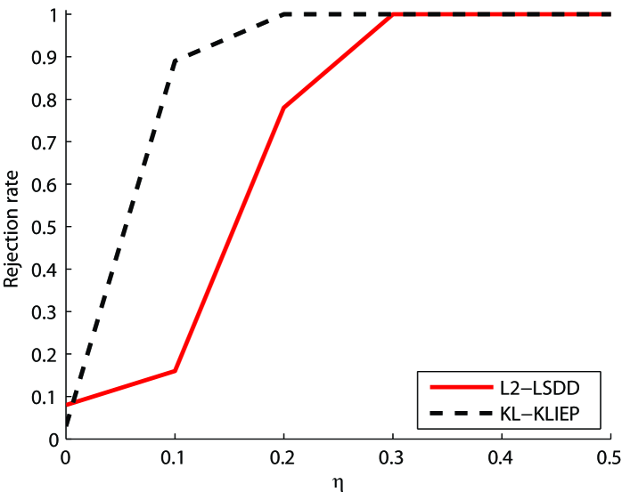
Figure 8: Two-sample test for outlier mean $\mu=10$ as functions of outlier rate $\eta$.

Finally, based on the permutation test procedure [book:Efron+Tibshirani:1993], we conduct hypothesis testing of the null hypothesis that densities $p$ and $p^{\prime}$ are the same. More specifically, we first compute a distance estimator for the original datasets ${\mathcal{X}}$ and ${\mathcal{X}}^{\prime}$ and obtain $\widehat{D}({\mathcal{X}},{\mathcal{X}}^{\prime})$. Next, we randomly permute the $|{\mathcal{X}}\cup{\mathcal{X}}^{\prime}|$ samples, and assign the first $|{\mathcal{X}}|$ samples to a set $\widetilde{{\mathcal{X}}}$ and the remaining $|{\mathcal{X}}^{\prime}|$ samples to another set $\widetilde{{\mathcal{X}}}^{\prime}$. Then we compute the distance estimator again using the randomly permuted datasets $\widetilde{{\mathcal{X}}}$ and $\widetilde{{\mathcal{X}}}^{\prime}$ and obtain $\widetilde{D}(\widetilde{{\mathcal{X}}},\widetilde{{\mathcal{X}}}^{\prime})$. Since $\widetilde{{\mathcal{X}}}$ and $\widetilde{{\mathcal{X}}}^{\prime}$ can be regarded as being drawn from the same distribution, $\widetilde{D}(\widetilde{{\mathcal{X}}},\widetilde{{\mathcal{X}}}^{\prime})$ would take a value close to zero. This random permutation procedure is repeated many times, and the distribution of $\widetilde{D}(\widetilde{{\mathcal{X}}},\widetilde{{\mathcal{X}}}^{\prime})$ under the null hypothesis (i.e., the two distributions are the same) is constructed. Finally, the p-value is approximated by evaluating the relative ranking of $\widehat{D}({\mathcal{X}},{\mathcal{X}}^{\prime})$ in the histogram of $\widetilde{D}(\widetilde{{\mathcal{X}}},\widetilde{{\mathcal{X}}}^{\prime})$. We set the significance level at $5\%$.

Figure 8 depicts the rejection rate of the null hypothesis for outlier rate $\eta=0.1$ and outlier mean $\mu=0,2,4,\ldots,10$, based on the $L^{2}$-distance estimated by LSDD and the KL-divergence estimated by KLIEP. This shows that the KLIEP-based test rejects the null hypothesis more frequently for large $\mu$, whereas the rejection rate of the LSDD-based test is kept almost constant even when $\mu$ is changed. This result implies that the two-sample test by LSDD is more robust against outliers (i.e., two distributions tend to be regarded as the same even in the presence of outliers) than the KLIEP-based test.

Figure 8 depicts the rejection rate of the null hypothesis for outlier mean $\mu=10$ for outlier rate $\eta=0,0.05,0.1,\ldots,0.35$. When $\eta=0$ (i.e., no outliers), both the LSDD-based test and the KLIEP-based test accept the null hypothesis with the designated significance level approximately. When $\eta=0.1$, the LSDD-based test still keeps a low rejection rate, whereas the KLIEP-based test tends to reject the null hypothesis. When $\eta\geq 0.3$, the LSDD-based test and the KLIEP-based test tend to reject the null hypothesis in a similar way.

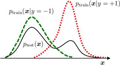
Figure 9: Schematic illustration of semi-supervised class-balance estimation.

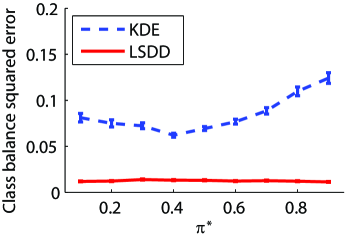
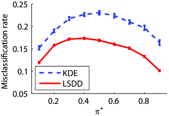
(a) Australian dataset

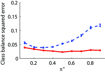
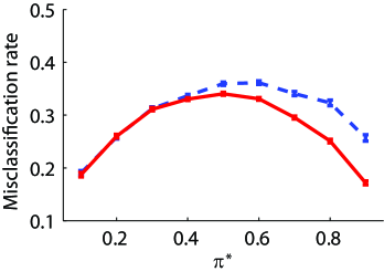
(b) Diabetes dataset

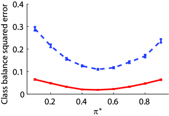
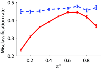
(c) German dataset

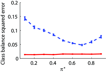
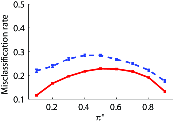
(d) Statlogheart dataset

Figure 10: Results of semi-supervised class-balance estimation. Left: Squared error of class balance estimation. Right: Misclassification error by a weighted regularized least-squares classifier.

4.2 Applications

Next, we apply LSDD to semi-supervised class-balance estimation under class prior change and change-point detection in time series.

4.2.1 Semi-Supervised Class-Balance Estimation

In real-world pattern recognition tasks, changes in class balance are often observed. Then significant estimation bias can be caused since the class balance in the training dataset does not reflect that of the test dataset.

Here, we consider a pattern recognition task of classifying pattern ${\boldsymbol{x}}\in\mathbb{R}^{d}$ to class $y\in\{+1,-1\}$. Our goal is to learn the class balance of a test dataset in a semi-supervised learning setup where unlabeled test samples are provided in addition to labeled training samples [book:Chapelle+etal:2006]. The class balance in the test set can be estimated by matching a mixture of class-wise training input densities,

$$\pi p_{\mathrm{train}}({\boldsymbol{x}}|y=+1)+(1-\pi)p_{\mathrm{train}}({\boldsymbol{x}}|y=-1),$$

with the test input density $p_{\mathrm{test}}({\boldsymbol{x}})$ [nc:Saerens+Latinne+Decaestecker:2002], where $\pi\in[0,1]$ is a mixing coefficient to learn. See Figure 9 for schematic illustration. Here, we use the $L^{2}$-distance estimated by LSDD and the difference of KDEs for this distribution matching.

We use four UCI benchmark datasets, where we randomly choose $20$ labeled training samples from each class and $50$ unlabeled test samples following true class-prior $\pi^{*}=0.1,0.2,\ldots,0.9$. Figure 10 plots the mean and standard error of the squared difference between true and estimated class balances $\pi$ and the misclassification error by a weighted regularized least-squares classifier [NATO-ASI:Rifkin+Yeo+Poggio:2003] over $1000$ runs. The results show that LSDD tends to provide better class-balance estimates, which are translated into lower classification errors.

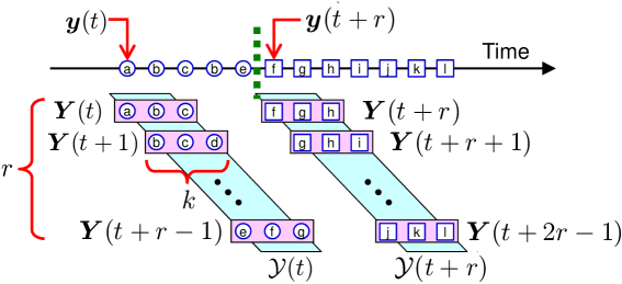
Figure 11: Schematic illustration of unsupervised change detection.

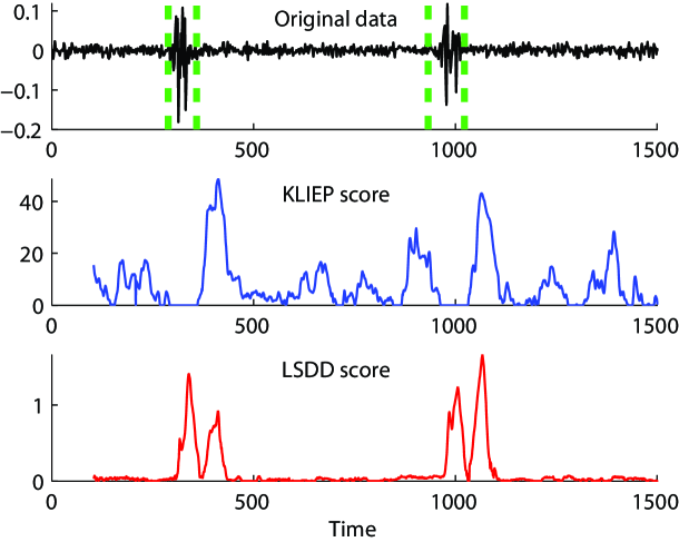
(a) Speech data

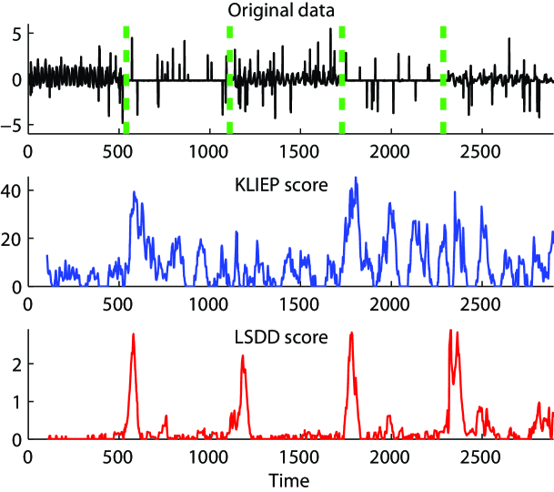
(b) Accelerometer data

Figure 12: Results of unsupervised change detection. Top: Original time-series. Middle: Change scores obtained by KLIEP. Bottom: Change scores obtained by LSDD.

4.2.2 Unsupervised Change Detection

The objective of change detection is to discover abrupt property changes behind time-series data.

Let ${\boldsymbol{y}}(t)\in\mathbb{R}^{m}$ be an $m$-dimensional time-series sample at time $t$, and let

$${\boldsymbol{Y}}(t):=[{\boldsymbol{y}}(t)^{\top},{\boldsymbol{y}}(t+1)^{\top},\ldots,{\boldsymbol{y}}(t+k-1)^{\top}]^{\top}\in\mathbb{R}^{km}$$

be a subsequence of time series at time $t$ with length $k$. We treat the subsequence ${\boldsymbol{Y}}(t)$ as a sample, instead of a single point ${\boldsymbol{y}}(t)$, by which time-dependent information can be incorporated naturally [SAM:Kawahara+Sugiyama:2012]. Let ${\mathcal{Y}}(t)$ be a set of $r$ retrospective subsequence samples starting at time $t$:

$${\mathcal{Y}}(t):=\{{{\boldsymbol{Y}}(t)},{\boldsymbol{Y}}(t+1),\ldots,{\boldsymbol{Y}}(t+r-1)\}.$$

Our strategy is to compute a certain dissimilarity measure between two consecutive segments ${\mathcal{Y}}(t)$ and ${\mathcal{Y}}(t+r)$, and use it as the plausibility of change points (see Figure 11). As a dissimilarity measure, we use the $L^{2}$-distance estimated by LSDD and the KL-divergence estimated by the KL importance estimation procedure (KLIEP) [AISM:Sugiyama+etal:2008, IEEE-IT:Nguyen+etal:2010]. We set $k=5$ and $r=50$.

First, we use the IPSJ SIG-SLP Corpora and Environments for Noisy Speech Recognition (CENSREC) dataset provided by the National Institute of Informatics, Japan, which records human voice in a noisy environment such as a restaurant. The top graph in Figure 12(a) displays the original time-series, where true change points were manually annotated. The bottom two graphs in Figure 12(a) plot change scores obtained by KLIEP and LSDD, showing that the LSDD-based change score indicates the existence of change points more clearly than the KLIEP-based change score.

Next, we use a dataset taken from the Human Activity Sensing Consortium (HASC) challenge 2011, which provides human activity information collected by portable three-axis accelerometers. Because the orientation of the accelerometers is not necessarily fixed, we take the $\ell_{2}$-norm of the 3-dimensional data. The top graph in Figure 12(b) displays the original time-series for a sequence of actions “jog”, “stay”, “stair down”, “stay”, and “stair up” (there exists $4$ change points at time $540$, $1110$, $1728$, and $2286$). The bottom two graphs in Figure 12(b) depict the change scores obtained by KLIEP and LSDD, showing that the LSDD score is much more stable and interpretable than the KLIEP score.

5 Conclusions

In this paper, we proposed a method for directly estimating the difference between two probability density functions without density estimation. The proposed method, called the least-squares density-difference (LSDD), was derived within a framework of kernel least-squares estimation, and its solution can be computed analytically in a computationally efficient and stable manner. Furthermore, LSDD is equipped with cross-validation, and thus all tuning parameters such as the kernel width and the regularization parameter can be systematically and objectively optimized. We showed the asymptotic normality of LSDD in a parametric setup and derived a finite-sample error bound for LSDD in a non-parametric setup. In both cases, LSDD achieves the optimal convergence rate.

We also proposed an $L^{2}$-distance estimator based on LSDD, which nicely cancels a bias caused by regularization. The LSDD-based $L^{2}$-distance estimator was experimentally shown to be more accurate than the difference of kernel density estimators and more robust against outliers than Kullback-Leibler divergence estimation.

Density-difference estimation is a novel research paradigm in machine learning, and we have given a simple but useful method for this emerging topic. Our future work will develop more powerful algorithms for density-difference estimation and explores a variety of applications.

Appendix A Technical Details of Non-Parametric Convergence Analysis in Section 2.3.2

First, we define linear operators $P_{n},P,P^{\prime}_{n},P^{\prime},Q_{n},Q$ as

$$P_{n}f:=\frac{1}{n}\sum_{i=1}^{n}f({\boldsymbol{x}}_{i}),~{}~{} Pf:=\int_{\mathbb{R}^{d}}f({\boldsymbol{x}})p({\boldsymbol{x}})\mathrm{d}{\boldsymbol{x}},$$

$$P^{\prime}_{n}f:=\frac{1}{n}\sum_{i=1}^{n}f({\boldsymbol{x}}^{\prime}_{i}),~{}~{} P^{\prime}f:=\int_{\mathbb{R}^{d}}f({\boldsymbol{x}})p^{\prime}({\boldsymbol{x}})\mathrm{d}{\boldsymbol{x}},$$

$$Q_{n}f:=P_{n}f-P^{\prime}_{n}f,~{}~{} Qf:=Pf-P^{\prime}f.$$

Let $\mathcal{H}_{\gamma}$ be an RKHS endowed with the Gaussian kernel with width $\gamma$:

$$k_{\gamma}({\boldsymbol{x}},{\boldsymbol{x}}^{\prime})=\exp\left(-\frac{\|{\boldsymbol{x}}-{\boldsymbol{x}}^{\prime}\|^{2}}{\gamma^{2}}\right).$$

A density-difference estimator $\widehat{f}$ is obtained as

$$\widehat{f}:=\mathop{\arg\min}_{f\in\mathcal{H}_{\gamma}}\left[\|f\|_{L^{2}(\mathbb{R}^{d})}^{2}-2Q_{n}f+\lambda\|f\|^{2}_{\mathcal{H}_{\gamma}}\right].$$

We assume the following conditions:

Assumption 1.

The densities are bounded: There exists $M$ such that

$$\|p\|_{\infty}\leq M\ \ \mbox{and}\ \ \|p^{\prime}\|_{\infty}\leq M.$$

The density difference $f=p-p^{\prime}$ is a member of Besov space with regularity $\alpha$: $f\in B_{2,\infty}^{\alpha}$ and, for $r=\lfloor\alpha\rfloor+1$ where $\lfloor\alpha\rfloor$ denotes the largest integer less than or equal to $\alpha$,

$$\|f\|_{B_{2,\infty}^{\alpha}}:=\|f\|_{L_{2}(\mathbb{R}^{d})}+\sup_{t>0}(t^{-\alpha}\omega_{r,L_{2}(\mathbb{R}^{d})}(f,t))<c,$$

where $B_{2,\infty}^{\alpha}$ is the Besov space with regularity $\alpha$ and $\omega_{r,L_{2}(\mathbb{R}^{d})}$ is the $r$-th modulus of smoothness (see ? (?) for the definitions).

Then we have the following theorem.

Theorem 2.

Suppose Assumption 1 is satisfied. Then, for all $\epsilon>0$ and $p\in(0,1)$, there exists a constant $K>0$ depending on $M,c,\epsilon,p$ such that for all $n\geq 1$, $\tau\geq 1$, and $\lambda>0$, the LSDD estimator $\widehat{f}$ in $\mathcal{H}_{\gamma}$ satisfies

$$\|\widehat{f}-f\|_{L^{2}(\mathbb{R}^{d})}^{2}\!+\!\lambda\|\widehat{f}\|_{\mathcal{H}_{\gamma}}^{2}\leq K\!\left(\lambda\gamma^{-d}\!+\!\gamma^{2\alpha}\!+\!\frac{\gamma^{-(1-p)(1+\epsilon)d}}{\lambda^{p}n}\!+\!\frac{\gamma^{-\frac{2(1-p)d}{1+p}(1+\epsilon+\frac{1-p}{4})}}{\lambda^{\frac{3p-p^{2}}{1+p}}n^{\frac{2}{1+p}}}\!+\!\frac{\tau}{n^{2}\lambda}\!+\!\frac{\tau}{n}\!\right)\!,$$

with probability not less than $1-4e^{-\tau}$.

To prove this, we utilize the technique developed in ? (?) for a regression problem.

Proof.

First, note that

$$\|\widehat{f}\|_{L^{2}(\mathbb{R}^{d})}^{2}-2Q_{n}\widehat{f}+\|f\|_{L^{2}(\mathbb{R}^{d})}^{2}+\lambda\|\widehat{f}\|_{\mathcal{H}_{\gamma}}^{2}\leq\|f_{0}\|_{L^{2}(\mathbb{R}^{d})}^{2}-2Q_{n}f_{0}+\|f\|_{L^{2}(\mathbb{R}^{d})}^{2}+\lambda\|f_{0}\|_{\mathcal{H}_{\gamma}}^{2}.$$

Therefore, we have

$$\!\!\!\!\!\!\!\!\!\!\!\!\!\|\widehat{f}-f\|_{L^{2}(\mathbb{R}^{d})}^{2}+\lambda\|\widehat{f}\|_{\mathcal{H}_{\gamma}}^{2}$$

$$=\|\widehat{f}\|_{L^{2}(\mathbb{R}^{d})}^{2}-2Q_{n}\widehat{f}+\|f\|_{L^{2}(\mathbb{R}^{d})}^{2}+2(Q_{n}-Q)\widehat{f}+\lambda\|\widehat{f}\|_{\mathcal{H}_{\gamma}}^{2}$$

$$\leq\|f_{0}\|_{L^{2}(\mathbb{R}^{d})}^{2}-2Q_{n}f_{0}+\|f\|_{L^{2}(\mathbb{R}^{d})}^{2}+2(Q_{n}-Q)\widehat{f}+\lambda\|\widehat{f}\|_{\mathcal{H}_{\gamma}}^{2}$$

$$=\|f_{0}\|_{L^{2}(\mathbb{R}^{d})}^{2}-2Qf_{0}+\|f\|_{L^{2}(\mathbb{R}^{d})}^{2}+2(Q_{n}-Q)(\widehat{f}-f_{0})+\lambda\|\widehat{f}\|_{\mathcal{H}_{\gamma}}^{2}$$

$$=\|f_{0}-f\|_{L^{2}(\mathbb{R}^{d})}^{2}+2(Q_{n}-Q)(\widehat{f}-f)+2(Q_{n}-Q)(f-f_{0})+\lambda\|\widehat{f}\|_{\mathcal{H}_{\gamma}}^{2}.$$ (16)

Let

$$K({\boldsymbol{x}}):=\sum_{j=1}^{r}{r\choose j}(-1)^{1-j}\frac{1}{j^{d}}\left(\frac{2}{\gamma\sqrt{\pi}}\right)^{\frac{d}{2}}\exp\left(-\frac{2\|{\boldsymbol{x}}\|^{2}}{j^{2}\gamma^{2}}\right),$$

and $\widetilde{f}({\boldsymbol{x}}):=(\gamma\sqrt{\pi})^{-\frac{d}{2}}f$. Using $K$ and $\widetilde{f}$, we define

$$f_{0}:=K*\widetilde{f}:=\int_{\mathbb{R}^{d}}\widetilde{f}(y)K(x-y)\mathrm{d}y,$$

i.e., $f_{0}$ is the convolution of $K$ and $\widetilde{f}$. Because of Lemma 2 in ? (?), we have $f_{0}\in\mathcal{H}_{\gamma}$ and

$$\|f_{0}\|_{\mathcal{H}_{\gamma}} \leq(2^{r}-1)\|\widetilde{f}\|_{L^{2}(\mathbb{R}^{d})}~{}~{}(\because\text{Lemma 2 of \immediate{\bf?} ({\bf?})})$$

$$\leq(2^{r}-1)(\gamma\sqrt{\pi})^{-\frac{d}{2}}\|f\|_{L^{2}(\mathbb{R}^{d})}$$

$$\leq(2^{r}-1)(\gamma\sqrt{\pi})^{-\frac{d}{2}}(\|p\|_{L^{2}(\mathbb{R}^{d})}+\|p^{\prime}\|_{L^{2}(\mathbb{R}^{d})})$$

$$\leq(2^{r}-1)(\gamma\sqrt{\pi})^{-\frac{d}{2}}2\sqrt{M}.$$ (17)

Moreover, Lemma 3 in ? (?) gives

$$\|f_{0}\|_{\infty}\leq(2^{r}-1)\|f\|_{\infty}\leq(2^{r}-1)M,$$ (18)

and Lemma 1 in ? (?) yields that there exists a constant $C_{r,2}$ such that

$$\|f_{0}-f\|_{L^{2}(\mathbb{R}^{d})}^{2}\leq C_{r,2}\omega_{r,L^{2}(\mathbb{R}^{d})}^{2}(f,\frac{\gamma}{2})\leq C_{r,2}c^{2}\gamma^{2\alpha}.$$ (19)

Now, following a similar line to Theorem 3 in ? (?), we can show that, for all $\epsilon>0$ and $p\in(0,1)$, there exists a constant $C_{\epsilon,p}$ such that

$$|(P_{n}-P)(\widehat{f}-f)|\leq\widehat{f}-f.$$

To bound this, we derive the tail probability of

$$(P_{n}-P)\left(\frac{\widehat{f}-f}{\|\widehat{f}-f\|_{L^{2}(\mathbb{R}^{d})}^{2}+\lambda\|\widehat{f}\|_{\mathcal{H}_{\gamma}}^{2}+r}\right),$$

where $r>0$ is a positive real such that $r>r^{*}$ for

$$r^{*}=\min_{f\in\mathcal{H}_{\gamma}}\|f-f\|_{L^{2}(\mathbb{R}^{d})}^{2}+\lambda\|f\|_{\mathcal{H}_{\gamma}}^{2}.$$

Let

$$g_{f,r}=\frac{f-f}{\|f-f\|_{L^{2}(\mathbb{R}^{d})}^{2}+\lambda\|f\|_{\mathcal{H}_{\gamma}}^{2}+r}$$

for $f\in\mathcal{H}_{\gamma}$ and $r>r^{*}$. Then we have

$$\|g_{f,r}\|_{\infty} \leq\frac{\|f\|_{\infty}+\|f\|_{\infty}}{\|f-f\|_{L^{2}(\mathbb{R}^{d})}^{2}+\lambda\|f\|_{\mathcal{H}_{\gamma}}^{2}+r}$$

$$\leq\frac{\|f\|_{\mathcal{H}_{\gamma}}+\|f\|_{\infty}}{\|f-f\|_{L^{2}(\mathbb{R}^{d})}^{2}+\lambda\|f\|_{\mathcal{H}_{\gamma}}^{2}+r}$$

$$\leq\frac{1}{\lambda\|f\|_{\mathcal{H}_{\gamma}}+r/\|f\|_{\mathcal{H}_{\gamma}}}+\frac{M}{r}\leq\frac{1}{2\sqrt{r\lambda}}+\frac{M}{r},$$

and

$$Pg_{f,r}^{2}=\frac{P(f-f)^{2}}{(\|f-f\|_{L^{2}(\mathbb{R}^{d})}^{2}+\lambda\|f\|_{\mathcal{H}_{\gamma}}^{2}+r)^{2}}\leq\frac{M\|f-f\|_{L^{2}(\mathbb{R}^{d})}^{2}}{(\|f-f\|_{L^{2}(\mathbb{R}^{d})}^{2}+\lambda\|f\|_{\mathcal{H}_{\gamma}}^{2}+r)^{2}}\leq\frac{M}{r}.$$

Here, let

$${\mathcal{F}}_{r}:=\{f\in\mathcal{H}_{\gamma}\mid\|f-f\|_{L^{2}(\mathbb{R}^{d})}^{2}+\lambda\|f\|_{\mathcal{H}_{\gamma}}^{2}\leq r\},$$

and we assume that there exists a function such that

$$\mathbb{E}\left[\sup_{f\in{\mathcal{F}}_{r}}|(P_{n}-P)(f-f)|\right]\leq\varphi_{n}(r),$$

where $\mathbb{E}$ denotes the expectation over all samples. Then, by the peeling device (see Theorem 7.7 in ?), we have

$$\mathbb{E}\sup_{f\in\mathcal{H}_{\gamma}}|(P_{n}-P)g_{f,r}|\leq\frac{8\varphi(r)}{r}.$$

Therefore, by Talagrand’s concentration inequality, we have

$$\mathrm{Pr}\left[\sup_{f\in\mathcal{H}_{\gamma}}|(P_{n}-P)g_{f,r}|<\frac{10\varphi_{n}(r)}{r}+\sqrt{\frac{2M\tau}{nr}}+\frac{14\tau}{3n}\left(\frac{1}{2\sqrt{r\lambda}}+\frac{M}{r}\right)\right]\geq 1-e^{-\tau},$$ (20)

where $\mathrm{Pr}[\cdot]$ denotes the probability of an event.

From now on, we give an upper bound of $\varphi_{n}$. The RKHS $\mathcal{H}_{\gamma}$ can embedded in arbitrary Sobolev space $W^{m}(\mathbb{R}^{d})$. Indeed, by the proof of Theorem 3.1 in ? (?), we have

$$\|f\|_{W^{m}(\mathbb{R}^{d})}\leq C_{m}\gamma^{-\frac{m}{2}+\frac{d}{4}}\|f\|_{\mathcal{H}_{\gamma}}$$

for all $f\in\mathcal{H}_{\gamma}$. Moreover, the theories of interpolation spaces give that, for all $f\in W^{m}(\mathbb{R}^{d})$, the supremum norm of $f$ can be bounded as

$$\|f\|_{\infty}\leq C_{m}^{\prime}\|f\|_{L^{2}(\mathbb{R}^{d})}^{1-\frac{d}{2m}}\|f\|_{W^{m}(\mathbb{R}^{d})}^{\frac{d}{2m}},$$

if $d<2m$. Here we set $m=\frac{d}{2p}$. Then we have

$$\|f\|_{\infty}\leq C_{p}^{\prime\prime}\|f\|_{L^{2}(\mathbb{R}^{d})}^{1-p}\|f\|_{\mathcal{H}_{\gamma}}^{p}\gamma^{-\frac{d(1-p)}{4}}.$$

Now, since ${\mathcal{F}}_{r}\subset(r/\lambda)^{1/2}{\mathcal{B}}_{\mathcal{H}_{\gamma}}$ and

$$P(f-f)^{2}\leq M\|f-f\|_{L^{2}(\mathbb{R}^{d})}^{2}\leq Mr~{}~{}~{}\mbox{for }f\in{\mathcal{F}}_{r}$$

hold from Theorem 7.16 and Theorem 7.34 in ? (?), we can take

$$\varphi_{n}(r)=\max\Bigg{\{} C_{1,p,\epsilon}\gamma^{-\frac{(1-p)(1+\epsilon)d}{2}}\left(\frac{r}{\lambda}\right)^{\frac{p}{2}}(Mr)^{\frac{1-p}{2}}n^{-1/2},$$

$$C_{2,p,\epsilon}\gamma^{-\frac{(1-p)(1+\epsilon)d}{1+p}}\left(\frac{r}{\lambda}\right)^{\frac{p}{1+p}}\left[\left(\frac{r}{\lambda}\right)^{\frac{p}{2}}\gamma^{-\frac{d(1-p)}{4}}r^{\frac{1-p}{2}}\right]^{\frac{1-p}{1+p}}n^{-1/(1+p)}\Bigg{\}},$$

where $\epsilon>0$ and $p\in(0,1)$ are arbitrary and $C_{1,p,\epsilon},C_{2,p,\epsilon}$ are constants depending on $p,\epsilon$. In the same way, we can also obtain a bound of $\sup_{f\in\mathcal{H}_{\gamma}}|(P^{\prime}_{n}-P^{\prime})g_{f,r}|$.

If we set $r$ to satisfy

$$\frac{1}{8}\geq\frac{10\varphi_{n}(r)}{r}+\sqrt{\frac{2M\tau}{nr}}+\frac{14\tau}{3n}\left(\frac{1}{2\sqrt{r\lambda}}+\frac{M}{r}\right),$$ (21)

then we have

$$|(Q_{n}-Q)(\widehat{f}-f)|\leq\frac{1}{4}\left(r+\|\widehat{f}-f\|_{L^{2}(\mathbb{R}^{d})}^{2}+\lambda\|\widehat{f}\|_{\mathcal{H}_{\gamma}}\right),$$ (22)

with probability $1-2e^{-\tau}$. To satisfy Eq.(21), it suffices to set

$$r=C\left(\frac{\gamma^{-(1-p)(1+\epsilon)d}}{\lambda^{p}n}+\frac{\gamma^{-\frac{2(1-p)d}{1+p}(1+\epsilon+\frac{1-p}{4})}}{\lambda^{\frac{3p-p^{2}}{1+p}}n^{\frac{2}{1+p}}}+\frac{\tau}{n^{2}\lambda}+\frac{\tau}{n}\right),$$ (23)

where $C$ is a sufficiently large constant depending on $M,\epsilon,p$.

Finally, we bound the term $(Q_{n}-Q)(f_{0}-f)$. By Bernstein’s inequality, we have

$$|(P_{n}-P)(f_{0}-f)| \leq C\left(\|f-f_{0}\|_{L_{2}(P)}\sqrt{\frac{\tau}{n}}+\frac{2^{r}M\tau}{n}\right)$$

$$\leq C\left(\sqrt{2M}\|f-f_{0}\|_{L^{2}(\mathbb{R}^{d})}\sqrt{\frac{\tau}{n}}+\frac{2^{r}M\tau}{n}\right)$$

$$\leq C\left(\|f-f_{0}\|_{L^{2}(\mathbb{R}^{d})}^{2}+\frac{2M\tau}{n}+\frac{2^{r}M\tau}{n}\right),$$ (24)

with probability $1-e^{-\tau}$, where $C$ is a universal constant. In a similar way, we can also obtain

$$|(P^{\prime}_{n}-P^{\prime})(f_{0}-f)|\leq C\left(\|f-f_{0}\|_{L^{2}(\mathbb{R}^{d})}^{2}+\frac{2M\tau}{n}+\frac{2^{r}M\tau}{n}\right).$$

Combining these inequalities, we have

$$|(Q_{n}-Q)(f_{0}-f)|\leq C\left(\|f-f_{0}\|_{L^{2}(\mathbb{R}^{d})}^{2}+\frac{2^{r}M\tau}{n}\right),$$ (25)

with probability $1-2e^{-\tau}$, where $C$ is a universal constant.

Substituting Eqs.(22) and (25) into Eq.(16), we have

$$\|\widehat{f}-f\|_{L^{2}(\mathbb{R}^{d})}^{2}+\lambda\|\widehat{f}\|_{\mathcal{H}_{\gamma}}^{2}$$

$$~{}~{}~{}\leq 2\left\{\|f_{0}-f\|_{L^{2}(\mathbb{R}^{d})}^{2}+C\left(\|f-f_{0}\|_{L^{2}(\mathbb{R}^{d})}^{2}+\frac{2^{r}M\tau}{n}\right)+r+\lambda\|f_{0}\|_{\mathcal{H}_{\gamma}}\right\},$$

with probability $1-4e^{-\tau}$. Moreover, by Eqs.(19) and (17), the right-hand side is further bounded by

$$\|\widehat{f}-f\|_{L^{2}(\mathbb{R}^{d})}^{2}+\lambda\|\widehat{f}\|_{\mathcal{H}_{\gamma}}^{2}\leq C\left\{\gamma^{2\alpha}+r+\lambda\gamma^{-d}+\frac{1+\tau}{n}\right\},$$

Finally, substituting (23) into the right-hand side, we have

$$\|\widehat{f}-f\|_{L^{2}(\mathbb{R}^{d})}^{2}+\lambda\|\widehat{f}\|_{\mathcal{H}_{\gamma}}^{2}$$

$$~{}~{}~{}\leq C\left\{\gamma^{2\alpha}+\frac{\gamma^{-(1-p)(1+\epsilon)d}}{\lambda^{p}n}+\frac{\gamma^{-\frac{2(1-p)d}{1+p}(1+\epsilon+\frac{1-p}{4})}}{\lambda^{\frac{3p-p^{2}}{1+p}}n^{\frac{2}{1+p}}}+\lambda\gamma^{-d}+\frac{\tau}{\lambda n^{2}}+\frac{\tau}{n}\right\},$$

with probability $1-4e^{-\tau}$ for $\tau\geq 1$. This gives the assertion. ∎

If we set

$$\lambda=n^{-\frac{2\alpha+d}{(2\alpha+d)(1+p)+(\epsilon-p+\epsilon p)}},~{}~{}\gamma=n^{-\frac{1}{(2\alpha+d)(1+p)+(\epsilon-p+\epsilon p)}},$$

and take $\epsilon,p$ sufficiently small, then we immediately have the following corollary.

Corollary 1.

Suppose Assumption 1 is satisfied. Then, for all $\rho,\rho^{\prime}>0$, there exists a constant $K>0$ depending on $M,c,\rho,\rho^{\prime}$ such that for all $n\geq 1$, $\tau\geq 1$, the density-difference estimator $\widehat{f}$ with appropriate choice of $\gamma$ and $\lambda$ satisfies

$$\|\widehat{f}-f\|_{L^{2}(\mathbb{R}^{d})}^{2}+\lambda\|\widehat{f}\|_{\mathcal{H}_{\gamma}}^{2}\leq K\left(n^{-\frac{2\alpha}{2\alpha+d}+\rho}+\frac{\tau}{n^{1-\rho^{\prime}}}\right),$$ (26)

with probability not less than $1-4e^{-\tau}$.

Note that $n^{-\frac{2\alpha}{2\alpha+d}}$ is the optimal learning rate to estimate a function in $B_{2,\infty}^{\alpha}$ [NIPS2011_0874]. Therefore, the density-difference estimator with a Gaussian kernel achieves the optimal learning rate by appropriately choosing the regularization parameter and the Gaussian width. Because the learning rate depends on $\alpha$, the LSDD estimator has an adaptivity to the smoothness of the true function.

Our analysis heavily relies on the techniques developed in ? (?) for a regression problem. The main difference is that the analysis in their paper involves a clipping procedure, which stems from the fact that the analyzed estimator requires an empirical approximation of the expectation of the square term. The Lipschitz continuity of the square function $f\mapsto f^{2}$ is utilized to investigate this term, and the clipping procedure is used to ensure the Lipschitz continuity. On the other hand, in the current paper, we can exactly compute $\|f\|_{L^{2}(\mathbb{R}^{d})}^{2}$ so that we do not need the Lipschitz continuity.

Appendix B Derivation of Eq.(13)

When $\lambda$ ($\geq 0$) is small, $\left({\boldsymbol{H}}+\lambda{\boldsymbol{I}}_{b}\right)^{-1}$ can be expanded as

$$\left({\boldsymbol{H}}+\lambda{\boldsymbol{I}}_{b}\right)^{-1}={\boldsymbol{H}}^{-1}-\lambda{\boldsymbol{H}}^{-2}+o_{p}(\lambda),$$

where $o_{p}$ denotes the probabilistic order. Then Eq.(12) can be expressed as

$$\!\!\!\!\!\!\!\!\!\!\beta{\widehat{{\boldsymbol{h}}}}^{\top}{\widehat{{\boldsymbol{\theta}}}}+(1-\beta){\widehat{{\boldsymbol{\theta}}}}^{\top}{\boldsymbol{H}}{\widehat{{\boldsymbol{\theta}}}}$$

$$=\beta{\widehat{{\boldsymbol{h}}}}^{\top}\left({\boldsymbol{H}}+\lambda{\boldsymbol{I}}_{b}\right)^{-1}{\widehat{{\boldsymbol{h}}}}+(1-\beta){\widehat{{\boldsymbol{h}}}}^{\top}\left({\boldsymbol{H}}+\lambda{\boldsymbol{I}}_{b}\right)^{-1}{\boldsymbol{H}}\left({\boldsymbol{H}}+\lambda{\boldsymbol{I}}_{b}\right)^{-1}{\widehat{{\boldsymbol{h}}}}$$

$$=\beta{\widehat{{\boldsymbol{h}}}}^{\top}{\boldsymbol{H}}^{-1}{\widehat{{\boldsymbol{h}}}}-\lambda\beta{\widehat{{\boldsymbol{h}}}}^{\top}{\boldsymbol{H}}^{-2}{\widehat{{\boldsymbol{h}}}}$$

$$\phantom{=}+(1-\beta){\widehat{{\boldsymbol{h}}}}^{\top}{\boldsymbol{H}}^{-1}{\widehat{{\boldsymbol{h}}}}-2\lambda(1-\beta){\widehat{{\boldsymbol{h}}}}^{\top}{\boldsymbol{H}}^{-2}{\widehat{{\boldsymbol{h}}}}+o_{p}(\lambda)$$

$$={\widehat{{\boldsymbol{h}}}}^{\top}{\boldsymbol{H}}^{-1}{\widehat{{\boldsymbol{h}}}}-\lambda(2-\beta){\widehat{{\boldsymbol{h}}}}^{\top}{\boldsymbol{H}}^{-2}{\widehat{{\boldsymbol{h}}}}+o_{p}(\lambda),$$

which concludes the proof.

Appendix C Derivation of Eq.(14)

Because $\mathbb{E}[{\widehat{{\boldsymbol{h}}}}]={\boldsymbol{h}}$, we have

$$\mathbb{E}[{\widehat{{\boldsymbol{h}}}}^{\top}{\boldsymbol{H}}^{-1}{\widehat{{\boldsymbol{h}}}}-{\boldsymbol{h}}^{\top}{\boldsymbol{H}}^{-1}{\boldsymbol{h}}] =\mathbb{E}[({\widehat{{\boldsymbol{h}}}}-{\boldsymbol{h}})^{\top}{\boldsymbol{H}}^{-1}({\widehat{{\boldsymbol{h}}}}-{\boldsymbol{h}})]$$

$$=\mathrm{tr}\left({\boldsymbol{H}}^{-1}\mathbb{E}[({\widehat{{\boldsymbol{h}}}}-{\boldsymbol{h}})({\widehat{{\boldsymbol{h}}}}-{\boldsymbol{h}})^{\top}]\right)$$

$$=\mathrm{tr}\left({\boldsymbol{H}}^{-1}\left(\frac{1}{n}{\boldsymbol{V}}_{p}[{\boldsymbol{\psi}}]+\frac{1}{n^{\prime}}{\boldsymbol{V}}_{p^{\prime}}[{\boldsymbol{\psi}}]\right)\right),$$

which concludes the proof.

References

- Anderson et al., 1994 Anderson et al.][1994]JMA:Anderson+etal:1994 Anderson, N., Hall, P., & Titterington, D. (1994). Two-sample test statistics for measuring discrepancies between two multivariate probability density functions using kernel-based density estimates. Journal of Multivariate Analysis, 50, 41–54.
- Aronszajn, 1950 Aronszajn][1950]AMS:Aronszajn:1950 Aronszajn, N. (1950). Theory of reproducing kernels. Transactions of the American Mathematical Society, 68, 337–404.
- Atif et al., 2003 Atif et al.][2003]ANBC:Atif+etal:2003 Atif, J., Ripoche, X., & Osorio, A. (2003). Non-rigid medical image registration by maximisation of quadratic mutual information. IEEE 29th Annual Northeast Bioengineering Conference (pp. 32–40).
- Baranchik, 1964 Baranchik][1964]TechRepo:Baranchik:1964 Baranchik, A. J. (1964). Multiple regression and estimation of the mean of a multivariate normal distribution (Technical Report 51). Department of Statistics, Stanford University, Stanford, CA, USA.
- Basu et al., 1998 Basu et al.][1998]Biometrika:Basu+etal:1998 Basu, A., Harris, I. R., Hjort, N. L., & Jones, M. C. (1998). Robust and efficient estimation by minimising a density power divergence. Biometrika, 85, 549–559.
- Besbeas & Morgan, 2004 Besbeas and Morgan][2004]CSDA:Besbeas+Morgan:2004 Besbeas, P., & Morgan, B. J. T. (2004). Integrated squared error estimation of normal mixtures. Computational Statistics & Data Analysis, 44, 517–526.
- Boser et al., 1992 Boser et al.][1992]COLT:Boser+etal:1992 Boser, B. E., Guyon, I. M., & Vapnik, V. N. (1992). A training algorithm for optimal margin classifiers. Proceedings of the Fifth Annual ACM Workshop on Computational Learning Theory (pp. 144–152). ACM Press.
- Chapelle et al., 2006 Chapelle et al.][2006]book:Chapelle+etal:2006 Chapelle, O., Schölkopf, B., & Zien, A. (Eds.). (2006). Semi-supervised learning. Cambridge, MA, USA: MIT Press.
- Cortes & Vapnik, 1995 Cortes and Vapnik][1995]mach:Cortes+Vapnik:1995 Cortes, C., & Vapnik, V. (1995). Support-vector networks. Machine Learning, 20, 273–297.
- Du Plessis & Sugiyama, 2012 Du Plessis and Sugiyama][2012]ICML:duPlessis+Sugiyama:2012 Du Plessis, M. C., & Sugiyama, M. (2012). Semi-supervised learning of class balance under class-prior change by distribution matching. Proceedings of 29th International Conference on Machine Learning (ICML2012). Edinburgh, Scotland.
- Duong et al., 2009 Duong et al.][2009]BJ:Duong+etal:2009 Duong, T., Koch, I., & Wand, M. P. (2009). Highest density difference region estimation with application to flow cytometric data. Biometrical Journal, 51, 504–521.
- Eberts & Steinwart, 2011 Eberts and Steinwart][2011]NIPS2011_0874 Eberts, M., & Steinwart, I. (2011). Optimal learning rates for least squares SVMs using Gaussian kernels. In J. Shawe-Taylor, R. S. Zemel, P. Bartlett, F. C. N. Pereira and K. Q. Weinberger (Eds.), Advances in neural information processing systems 24, 1539–1547.
- Efron & Tibshirani, 1993 Efron and Tibshirani][1993]book:Efron+Tibshirani:1993 Efron, B., & Tibshirani, R. J. (1993). An introduction to the bootstrap. New York, NY, USA: Chapman & Hall/CRC.
- Farrell, 1972 Farrell][1972]AMS:Farrell:1972 Farrell, R. H. (1972). On the best obtainable asymptotic rates of convergence in estimation of a density function at a point. The Annals of Mathematical Statistics, 43, 170–180.
- Gray & Principe, 2010 Gray and Principe][2010]SPIE:Gray+Principe:2010 Gray, D. M., & Principe, J. C. (2010). Quadratic mutual information for dimensionality reduction and classification. Proceedings of SPIE (p. 76960D).
- Gretton et al., 2009 Gretton et al.][2009]Inbook:Gretton+etal:2009 Gretton, A., Smola, A., Huang, J., Schmittfull, M., Borgwardt, K., & Schölkopf, B. (2009). Covariate shift by kernel mean matching. In J. Quiñonero-Candela, M. Sugiyama, A. Schwaighofer and N. Lawrence (Eds.), Dataset shift in machine learning, chapter 8, 131–160. Cambridge, MA, USA: MIT Press.
- Hall & Wand, 1988 Hall and Wand][1988]Biometrika:Hall+Wand:1988 Hall, P., & Wand, M. P. (1988). On nonparametric discrimination using density differences. Biometrika, 75, 541–547.
- Härdle et al., 2004 Härdle et al.][2004]book:Haerdle+etal:2004 Härdle, W., Müller, M., Sperlich, S., & Werwatz, A. (2004). Nonparametric and semiparametric models. Berlin, Germany: Springer.
- Kanamori et al., 2009 Kanamori et al.][2009]JMLR:Kanamori+etal:2009 Kanamori, T., Hido, S., & Sugiyama, M. (2009). A least-squares approach to direct importance estimation. Journal of Machine Learning Research, 10, 1391–1445.
- Kanamori et al., 2012 Kanamori et al.][2012]ML:Kanamori+etal:2012 Kanamori, T., Suzuki, T., & Sugiyama, M. (2012). Statistical analysis of kernel-based least-squares density-ratio estimation. Machine Learning, 86, 335–367.
- Kawahara & Sugiyama, 2012 Kawahara and Sugiyama][2012]SAM:Kawahara+Sugiyama:2012 Kawahara, Y., & Sugiyama, M. (2012). Sequential change-point detection based on direct density-ratio estimation. Statistical Analysis and Data Mining, 5, 114–127.
- Kullback & Leibler, 1951 Kullback and Leibler][1951]Annals-Math-Stat:Kullback+Leibler:1951 Kullback, S., & Leibler, R. A. (1951). On information and sufficiency. The Annals of Mathematical Statistics, 22, 79–86.
- Liu et al., 2010 Liu et al.][2010]PR:Liu+eta:2010 Liu, B., Cheng, H. D., Huang, J., Tian, J., Tang, X., & Liu, J. (2010). Probability density difference-based active contour for ultrasound image segmentation. Pattern Recognition, 43, 2028–2042.
- Liu et al., 2012 Liu et al.][2012]arXiv:Song+etal:2012 Liu, S., Yamada, M., Collier, N., & Sugiyama, M. (2012). Change-point detection in time-series data by relative density-ratio estimation (Technical Report 1203.0453). arXiv.
- Matsugu et al., 2011 Matsugu et al.][2011]VECTaR:Yamanaka+etal:2011 Matsugu, M., Yamanaka, M., & Sugiyama, M. (2011). Detection of activities and events without explicit categorization. Proceedings of the 3rd International Workshop on Video Event Categorization, Tagging and Retrieval for Real-World Applications (VECTaR2011) (pp. 1532–1539). Barcelona, Spain.
- Nguyen et al., 2010 Nguyen et al.][2010]IEEE-IT:Nguyen+etal:2010 Nguyen, X., Wainwright, M. J., & Jordan, M. I. (2010). Estimating divergence functionals and the likelihood ratio by convex risk minimization. IEEE Transactions on Information Theory, 56, 5847–5861.
- Parzen, 1962 Parzen][1962]AMS:Parzen:1962 Parzen, E. (1962). On the estimation of a probability density function and mode. The Annals of Mathematical Statistics, 33, 1065–1076.
- Pérez-Cruz, 2008 Pérez-Cruz][2008]ISIT:Perez-Cruz:2008 Pérez-Cruz, F. (2008). Kullback-Leibler divergence estimation of continuous distributions. Proceedings of IEEE International Symposium on Information Theory (pp. 1666–1670). Nice, France.
- Qin, 1998 Qin][1998]Biometrika:Qin:1998 Qin, J. (1998). Inferences for case-control and semiparametric two-sample density ratio models. Biometrika, 85, 619–630.
- Rao, 1965 Rao][1965]book:Rao:1965 Rao, C. R. (1965). Linear statistical inference and its applications. New York, NY, USA: Wiley.
- Rifkin et al., 2003 Rifkin et al.][2003]NATO-ASI:Rifkin+Yeo+Poggio:2003 Rifkin, R., Yeo, G., & Poggio, T. (2003). Regularized least-squares classification. Advances in Learning Theory: Methods, Models and Applications (pp. 131–154). Amsterdam, the Netherlands: IOS Press.
- Rockafellar, 1970 Rockafellar][1970]book:Rockafellar:1970 Rockafellar, R. T. (1970). Convex analysis. Princeton, NJ, USA: Princeton University Press.
- Saerens et al., 2002 Saerens et al.][2002]nc:Saerens+Latinne+Decaestecker:2002 Saerens, M., Latinne, P., & Decaestecker, C. (2002). Adjusting the outputs of a classifier to new a priori probabilities: A simple procedure. Neural Computation, 14, 21–41.
- Scott, 2001 Scott][2001]Tech:Scott:2001 Scott, D. W. (2001). Parametric statistical modeling by minimum integrated square error. Technometrics, 43, 274–285.
- Silva & Narayanan, 2010 Silva and Narayanan][2010]JSPI:Silva+Narayanan:2010 Silva, J., & Narayanan, S. S. (2010). Information divergence estimation based on data-dependent partitions. Journal of Statistical Planning and Inference, 140, 3180–3198.
- Silverman, 1986 Silverman][1986]book:Silverman:1986 Silverman, B. W. (1986). Density estimation for statistics and data analysis. London, UK: Chapman and Hall.
- Steinwart & Christmann, 2008 Steinwart and Christmann][2008]Book:Steinwart:2008 Steinwart, I., & Christmann, A. (2008). Support vector machines. New York, NY, USA: Springer.
- Steinwart & Scovel, 2004 Steinwart and Scovel][2004]AS:Steinwart+Scovel:2004 Steinwart, I., & Scovel, C. (2004). Fast rates for support vector machines using Gaussian kernels. The Annals of Statistics, 35, 575–607.
- Sugiyama et al., 2012a Sugiyama et al.][2012a]book:Sugiyama+etal:2012 Sugiyama, M., Suzuki, T., & Kanamori, T. (2012a). Density ratio estimation in machine learning. Cambridge, UK: Cambridge University Press.
- Sugiyama et al., 2012b Sugiyama et al.][2012b]AISM:Sugiyama+etal:2012 Sugiyama, M., Suzuki, T., & Kanamori, T. (2012b). Density ratio matching under the Bregman divergence: A unified framework of density ratio estimation. Annals of the Institute of Statistical Mathematics. to appear.
- Sugiyama et al., 2008 Sugiyama et al.][2008]AISM:Sugiyama+etal:2008 Sugiyama, M., Suzuki, T., Nakajima, S., Kashima, H., von Bünau, P., & Kawanabe, M. (2008). Direct importance estimation for covariate shift adaptation. Annals of the Institute of Statistical Mathematics, 60, 699–746.
- Torkkola, 2003 Torkkola][2003]JMLR:Torkkola:2003 Torkkola, K. (2003). Feature extraction by non-parametric mutual information maximization. Journal of Machine Learning Research, 3, 1415–1438.
- Vapnik, 1998 Vapnik][1998]book:Vapnik:1998 Vapnik, V. N. (1998). Statistical learning theory. New York, NY, USA: Wiley.
- Wang et al., 2005 Wang et al.][2005]IEEE-IT:Wang+etal:2005 Wang, Q., Kulkarmi, S. R., & Verdú, S. (2005). Divergence estimation of contiunous distributions based on data-dependent partitions. IEEE Transactions on Information Theory, 51, 3064–3074.