Quantum-like model of behavioral response computation using neural oscillators

Abstract

In this paper we propose the use of neural interference as the origin of quantum-like effects in the brain. We do so by using a neural oscillator model consistent with neurophysiological data. The model used was shown elsewhere to reproduce well the predictions of behavioral stimulus-response theory. The quantum-like effects are brought about by the spreading activation of incompatible oscillators, leading to an interference-like effect mediated by inhibitory and excitatory synapses.

1 Introduction

Quantum mechanics is one of the most successful scientific theories in history. From it, detailed predictions and extremely precise descriptions of a wide range of physical systems are given. Thus, it is not surprising that researchers from social and behavioral sciences disciplines started asking whether the apparatus of quantum mechanics could be useful to them (Khrennikov, 2010). In applying the quantum formalism, most researchers do not claim to have found social or behavioral phenomena that are determined by the physical laws of quantum mechanics (Bruza et al., 2009). Instead, they claim that by using the representation of states in a Hilbert space, together with the corresponding non-Kolmogorovian interference of probabilities, a better description of observed phenomena could be achieved. To distinguish the idea that the formalism describing a system is quantum without requiring the system itself to be, researchers often use the term quantum-like.

One of the first applications of quantum-like dynamics outside of physics was in finances (Baaquie, 1997; Haven, 2002) and in decision making (Busemeyer et al., 2006; Aerts, 2009). In economy, Baaquie (1997) showed that a more general form of the Black-Scholes option pricing equation was given by a Schrödinger-type equation, and Haven (2002) linked the equivalent of the Plank constant to the existence of arbitrage in the model. In psychology, most of the initial effort was focused on using quantum-like dynamics and Hilbert-space formalisms to describe discrepancies between empirical data and “classical” models using standard probability theory (see, for example, Aerts (2009); Asano et al. (2010); Busemeyer et al. (2006); Busemeyer and Wang (2007); Busemeyer et al. (2009); Khrennikov (2009); Khrennikov and Haven (2009); Khrennikov (2011)).

To try to describe quantum-like effects in cognitive sciences, in a recent paper Khrennikov (2011) used a classical electromagnetic-field model for the mental processing of information. In it, Khrennikov argues that the collective activity of neurons involved in mental processing produces electromagnetic signals. Such signals then propagate in the brain, leading to interference and the appearance of quantum-like correlations. He used this model to show how quantum-like effects help understand the binding problem.

In this paper we set forth a neural oscillator model exhibiting many of the characteristics of Khrennikov’s. The neural model we employ was initially proposed as an attempt to obtain behavioral stimulus-response theory from the neuronal activities in the brain (Suppes et al., 2012). There are many different ways to use neural oscillators to model learning (see Vassilieva et al., 2011, and references therein), but to our knowledge, this is the only one that makes a clear connection between neural oscillator computations and the behavioral responses. Furthermore, the model is simple enough to help understand the basic principles behind the computation of a response from a stimulus without compromising the neurophysiological interpretation of it. This must be emphasized, as most neural models constructed from a neurophysiological basis are so computationally intensive and complex that it is very hard to understand why or how one response was select instead of another. We shall see later that this is not the case with Suppes et al. (2012).

As with Khrennikov’s electromagnetic field model, our model has many quantum-like characteristics, such as signaling, superposition, and interference. However, it does not rely on the propagation of electromagnetic fields in the brain. Instead, we show that these quantum-like effects could be obtained by directly considering the interference of the activities of collections of firing neurons coupled via inhibitory and excitatory synapses. In particular, we show a violation of Savage’s sure-thing principle, often cited as an example of quantum-like behavior.

This paper is organized as follows. In section 2 we introduce Suppes, de Barros, and Oas’s (2012) oscillator model, with special emphasis to its neurophysiological interpretation and connection to SR theory. Then, in section 3.1, we present a contextual theory of quantum-like phenomena coming from classical interference of waves (de Barros and Suppes, 2009). Finally, in section 2 we show computer simulations of neural oscillators and how they fit some quantum-like experimental data in the literature. We end with some remarks.

2 Neural oscillator model of SR-theory

In this section, we delineate the modeling of SR theory by neural oscillators. This section is divided into three parts. First, in subsection 2.1 we sketch the mathematical version of behavioral SR theory we model. Then, in subsection 2.2 we present the model of Suppes et al. (2012) in a qualitative way. Finally, in subsection 2.3 we give a mathematical description of the oscillator model. Our goal is not to be exhaustive, but only to focus on the main features of the model that are relevant for the emergence of quantum-like effects derived later. Readers interested in more detail are referred to (Suppes et al., 2012; de Barros et al., 2012).

2.1 Review of SR theory

Stimulus-response theory (or SR theory) is one of the most successful behavioral learning theories in psychology (Suppes and Atkinson, 1960). Among the many reasons for its success, it has been shown to fit well empirical data in a variety of experiments. This fitting requires few parameters (the learning probability $c$ and the number of stimuli), giving it strong prediction powers from few assumptions. Also, because it requires a rigid trial structure, its concepts can be formally axiomatized, resulting in many important non-trivial experiments. Finally, despite its simplicity, SR theory is rich enough such that even language can be represented within its framework (Suppes, 2002). Thus, SR theory presents an ideal mathematical structure to be modeled at a neuronal level.

Here we present the mathematical version of SR theory for a continuum of responses, formalized in terms of a stochastic process (here we follow Suppes et al., 2012). Let $\left(\Omega,{\cal F},P\right)$ be a probability space, and let $\mathbf{Z}$, $\mathbf{S}$, $\mathbf{R}$, and $\mathbf{E}$ be random variables, with $\mathbf{Z}:\Omega\rightarrow E^{\left|S\right|}$ $\mathbf{S}:\Omega\rightarrow S$, $\mathbf{R}:\Omega\rightarrow R$, and $\mathbf{E}:\Omega\rightarrow E$, where $S$ is the set of stimuli, $R$ the set of responses, and $E$ the set of reinforcements. Then a trial in SR theory has the following structure:

$$\mathbf{Z}_{n}\rightarrow\mathbf{S}_{n}\rightarrow\mathbf{R}_{n}\rightarrow\mathbf{E}_{n}\rightarrow\mathbf{Z}_{n+1}.$$ (1)

Intuitively, the trial structure works the following way. Trial $n$ starts with a certain state of conditioning and a sampled stimulus. Once a stimulus is sampled, a response is computed according to the state of conditioning. Then, reinforcement follows, which can lead (with probability $c$) to a new state of conditioning for trial $n+1$ . In more detail, at the beginning of a trial, the state of conditioning is represented by the random variable $\mathbf{Z}_{n}=\left(z_{1}^{\left(n\right)},\ldots,z_{m}^{\left(n\right)}\right)$. The vector $\left(z_{1}^{\left(n\right)},\ldots,z_{m}^{\left(n\right)}\right)$ associates to each stimuli $s_{i}\in S$, $i=1,\ldots,m$, where $m=\left|S\right|$ is the cardinality of $S$, a value $z_{i}^{\left(n\right)}$ on trial $n$. Once a stimulus $\mathbf{S}_{n}=s_{i}$ is sampled with probability $P\left(\mathbf{S}_{n}=s_{i}|s_{i}\epsilon S\right)=\dfrac{1}{m}$, its corresponding $z_{i}^{\left(n\right)}$ determines the probability of responses in $R$ by the probability distribution $K\left(r|z_{i}^{\left(n\right)}\right)$, i.e. $P\left(a_{1}\leq\mathbf{R}_{n}\leq a_{2}|\mathbf{S}_{n}=s_{i},\mathbf{Z}_{n,i}=z_{i}^{\left(n\right)}\right)=\int_{a_{1}}^{a_{2}}k\left(x|z_{i}^{\left(n\right)}\right)dx$, where $k\left(x|z_{i}^{\left(n\right)}\right)$ is the probability density associate to the distribution, and where $\mathbf{Z}_{n,i}$ is the $i$-th component of the vector $\left(z_{1}^{\left(n\right)},\ldots,z_{m}^{\left(n\right)}\right)$. The probability distribution $K\left(r|z_{i}^{\left(n\right)}\right)$ is the smearing distribution, and it is determined by its variance and mode $z_{i}^{\left(n\right)}$ . The next step is the reinforcement $\mathbf{E}_{n}$, which is effective with probability $c$, i.e. $P\left(\mathbf{Z}_{n+1,i}=y|\mathbf{S}_{n}=s_{i},\mathbf{E}_{n}=y,\mathbf{Z}_{n,i}=z_{i}^{\left(n\right)}\right)=c$ and $P\left(\mathbf{Z}_{n+1,i}=z_{i}^{\left(n\right)}|\mathbf{S}_{n}=s_{i},\mathbf{E}_{n}=y,\mathbf{Z}_{n,i}=z_{i}^{\left(n\right)}\right)=1-c$. The trial ends with a new (with probability $c$) state of conditioning $\mathbf{Z}_{n+1}$.

2.2 Qualitative description of oscillator model

Because of its focus on behavioral outcomes, mathematical SR theory does not provide a clear connection to the internal processing of information by the brain. To bridge this gap, Suppes et al. (2012) proposed a neural-oscillator based response computation model able to reproduce the main stochastic features of SR theory, including the conditional probabilities for a continuum of responses. It is this model that we describe qualitatively in this subsection.

In SR theory, a trial is given by the sequence in (1). In the oscillator model, with the exception of $\mathbf{Z}_{n}$, each random variable is represented by a corresponding oscillator. To better understand the model, let us examine each step of an SR trial in terms of oscillators.

Let us start with the sampling of a stimulus, $\mathbf{S}_{n}$. At the beginning of a trial, a (distal) stimulus is presented. Through the perceptual system processing, it reaches an area of the brain where it produces a somewhat synchronized firing of a set of neurons. This set of firing neurons is what we think as the activation of the sampled stimulus oscillator, $O_{s}\left(t\right)$. The oscillator $O_{s}\left(t\right)$ is a simplified description of the semi-periodic activity of the collection of (perhaps thousands of) neurons.

We now turn to the computation of a response, $\mathbf{R}_{n}$. For simplicity, we first consider two possible responses, $R_{1}$ and $R_{2}$ (i.e. $R=\left\{R_{1},R_{2}\right\}$); later we show how we generalize to any number of to a continuum of responses. Once $O_{s}\left(t\right)$ is activated, its couplings to other neurons may lead to a spreading of its activation to other sets of neurons, including the response neurons. Say we can split the neurons activated by $O_{s}\left(t\right)$’s couplings into two sets, one representing $R_{1}$ and the other $R_{2}$. Since those neurons were activated, as the stimulus neurons, they fire in relative synchrony, and can be represented by the oscillators $O_{r_{1}}\left(t\right)$ and $O_{r_{2}}\left(t\right)$. Of course, the activation of both $O_{r_{1}}\left(t\right)$ and $O_{r_{2}}\left(t\right)$ is not enough for the computation of a response. To see how a response is computed in the oscillator model from $O_{r_{1}}\left(t\right)$ and $O_{r_{2}}\left(t\right)$, we need think of what happens if two oscillators are in-phase or out-of-phase. When two neural oscillators are in phase, the firing of one adds to the firing of the other, perhaps reaching a certain response threshold; if they are out of phase, such threshold may not be reached, as the firings do not add above their activated intensities. So, a response is chosen depending on the relative phases of the oscillators. If $O_{s}\left(t\right)$ is in phase with $O_{r_{1}}\left(t\right)$ and out of phase with $O_{r_{2}}\left(t\right)$, response $R_{1}$ is selected. Which response is selected depends on the actual couplings between $O_{s}\left(t\right)$, $O_{r_{1}}\left(t\right)$, and $O_{r_{2}}\left(t\right)$ (see next subsection for details).

We can now talk about $\mathbf{E}_{n}$, $\mathbf{Z}_{n}$, and $\mathbf{Z}_{n+1}$. Since the selected response is determined by the couplings between neural oscillators, clearly the state of conditioning $\mathbf{Z}_{n}$ depends on those couplings. Therefore, on the oscillator model, saying that a trial starts with a state of conditioning $\mathbf{Z}_{n}$ is the same as saying that a trial starts with a set of synaptic connections between the neurons belonging to the ensembles representing the activated stimulus and responses. But, as the reinforcement $\mathbf{E}_{n}$ may change $\mathbf{Z}_{n}$ into a different state of conditioning, $\mathbf{Z}_{n+1}$, it follows that during reinforcement the neural couplings need to change. So, in the oscillator model, such couplings change when a neural reinforcement oscillator (corresponding to the activation of an ensemble of neurons representing reinforcement) interacts with the stimulus and response oscillators, thus driving a Hebb-like change in synaptic connection, resulting in learning.

The previous paragraphs summarize qualitatively the model, but there are three points that need to be further discussed before we proceed to the quantitative description. First, since neural oscillators correspond to a tremendous dimensional reduction in the neuronal dynamical system, we need to justify their use. Second, as it is crucial for the model, an argument needs to be made as to how oscillators synchronize. Finally, we should the two-response case, but how can a finite number of oscillators encode a large number of responses, possibly a continuum of responses?

Why neural oscillators? First, we note that Suppes et al. (2012) does not propose the use of neural oscillators for any type of modeling. Instead, they argue that if we are interested in higher cognitive functions, such as language, it can be showed that they can be represented on electroencephalogram (EEG) oscillation patterns (see Suppes, 2002, Chapter 8, and corresponding references). But EEG signals are the result of a large assembly of neurons firing synchronously or quasi-synchronously (Nunez and Srinivasan, 2006). Thus, we can think of a word as represented in the brain by a set of coupled neurons. When this word is activated by an external stimulus, this set of neurons fire coherently. Such an ensemble of synchronizing neurons could, in first approximation, be represented by a periodic function $F_{T}(t)$, where $T$ is the period of the function. So, for Suppes et al. (2012) a neural oscillator is simply a set of firing neurons represented by such periodic functions, and a good candidate as a unit of processing of information in the brain.

It must be emphasized that representing a collection of neurons by a periodic function, as we did above, does not mean that all neurons fire simultaneously. It just means that the firing frequencies of individual neurons become very close to each other. But neurons with the same frequency do not need to fire at the same times. In other words, they may synchronize out of phase. But, more importantly, once they synchronize, the initial dynamical system with thousands of degrees of freedom become describable by a single dynamical variable, the periodic function $F_{T}(t)$. It is this dramatic dimensional reduction that allows us to produce a model whose behavior we can understand in certain specific situations.

We now move to the question of how neural oscillators synchronize. Let us first look at the qualitative behavior of individual neurons in two ensembles, $A$ and $B$, each with a large number of neurons firing coherently. Let $n_{A}$ be a single neuron in ensemble $A$ firing with period $T_{A}$, and let $n_{B}$ be another neuron in $B$ firing with period $T_{B}$. Let $t^{\prime}$ be a particular time such that $n_{B}$ would fire if $A$ were not activated, i.e. the time it would fire because of its natural periodicity $T_{B}$. If $n_{A}$ and $n_{B}$ are synaptically coupled, a firing of $n_{A}$ at a time $t\lessapprox t^{\prime}$ would anticipate $n_{B}$’s firing to a time $t^{\prime\prime}$ closer to $t$, thus approaching the timing of firing for both neurons. If more neurons from ensemble $A$ are coupled to $n_{B}$, the stronger the effect of anticipating its firing time. Furthermore, since $n_{B}$ is also coupled to neurons in $A$, its firing has the same effect on $A$ (though this effect does not need to be symmetric). So, the couplings between $A$ and $B$ lead both periods $T_{A}$ and $T_{B}$ to approach each other, i.e., $A$ and $B$ synchronize. In fact, it is possible to prove mathematically that, under the right conditions, if the number of neurons is large enough, the sum of the several weak synaptic interactions can cause a strong effect, making all neurons fire close together (Izhikevich, 2007). In other words, even when weakly coupled, two neural ensembles represented by oscillators may synchronize.

We end this subsection with the representation of a continuum of responses in terms of neural oscillators. Continuum of responses show up in some behavioral experiments. For example, a possible task could be to predict the position of an airplane on a radar screen (represented by a flashing dot appearing periodically) after observing its position for several trials. Since the radar position can be anywhere in the screen, this cannot be represented by a discrete set of responses.

So, how could we represent a continuum of responses with neural oscillators? With a discrete number of responses, what we did was to create a representation for each response in terms of a distinct oscillator (in our example above, $O_{r_{1}}\left(t\right)$ and $O_{r_{2}}\left(t\right)$). But this approach would lead to an uncountable number of neural oscillators for the continuum case, clearly a physically unreasonable assumption. But there is another alternative. When we used oscillators for the two responses, we thought about $O_{r_{1}}\left(t\right)$ and $O_{r_{2}}\left(t\right)$ as being either in phase or out of phase with $O_{s}\left(t\right)$. However, they do not need to be in perfect phase. In the next section, we show that by using specific differences of phase between $O_{r_{1}}\left(t\right)$ and $O_{r_{2}}\left(t\right)$ and $O_{s}\left(t\right)$, we can control the amount of “intensity” of a neural activation on each oscillator. This relative intensity between $O_{r_{1}}\left(t\right)$ and $O_{r_{2}}\left(t\right)$ can be used as a measure of how close a response is to either $R_{1}$ or $R_{2}$; in other words, we can think of the response as being between $R_{1}$ and $R_{2}$, which would correspond to a continuum. So, by thinking of $R_{1}$ and $R_{2}$ as extremes in a possible range of responses in a continuum interval, the relative intensities of $O_{r_{1}}\left(t\right)$ and $O_{r_{2}}\left(t\right)$, given by their phase relation with $O_{s}\left(t\right)$, could code any response in between.

2.3 Quantitative description of the oscillator model

We now turn to a more rigorous mathematical description. Our underlying assumption is that we have two neural ensembles $A$ and $B$ described by periodic functions $F_{T_{A}}\left(t\right)$ and $F_{T_{B}}\left(t\right)$ with periods $T_{A}$ and $T_{B}$, respectively. Without loss of generality in our argument, we assume that $F_{T_{A}}\left(t\right)$ and $F_{T_{B}}\left(t\right)$ have the same shape, i.e., there exists a constant $c$ such that $F_{T_{A}}\left(t\right)=F_{T_{B}}\left(tc\right)$. A simple way to describe the synchronization of $A$ and $B$ is to rewrite the time argument in the functions, rewriting them as $F_{T_{A}}\left(t\alpha_{A}\right)$ and $F_{T_{B}}\left(t\alpha_{B}\right)$. Clearly, if no couplings exist between $A$ and $B$, their dynamics is not modified and $\alpha_{A}=\alpha_{B}=1$. However, when the ensembles are couples, $\alpha_{A}$ and $\alpha_{B}$ are a function of time, their synchronization means that they evolve such that $F_{T_{A}}\left(t\alpha_{A}\left(t\right)\right)=F_{T_{B}}\left(t\alpha_{B}\left(t\right)\right)$. Thus, when we are studying the dynamics of coupled neural oscillators, it suffices to study the dynamics of the arguments of $F_{T_{A}}$ and $F_{T_{B}}$ above, which we call their phases.

To illustrate this point, let us imagine a simple case where when there is no interaction $A$ follows a harmonic oscillator with angular frequency $\omega_{A}=2\pi/T_{A}$. Then $F_{T_{A}}\left(t\right)=A\cos\left(\omega_{A}t+\delta_{A}\right)$, where and $\delta_{A}$ is a constant, and expressions hold for $F_{T_{B}}\left(t\right)$. Following the above paragraph, we rewrite

$$F_{T_{A}}\left(t\right)=A\cos\left(\varphi_{A}\left(t\right)\right),$$

where

$$\varphi_{A}\left(t\right)=\omega_{A}t+\delta_{A}$$ (2)

is the phase. Let us now focus on the phase dynamics.

For a set of coupled phase oscillators, Kuramoto (1984) proposed a simple set of dynamical equations for $\varphi_{A}\left(t\right)$. To better understand them, let us assume that in the absence of interactions $\varphi_{A}$ evolves according to (2). Thus, the differential equation describing $\varphi_{A}$ would be

$$\frac{d\varphi_{A}\left(t\right)}{dt}=\omega_{A},$$ (3)

and for $\varphi_{B}$,

$$\frac{d\varphi_{B}\left(t\right)}{dt}=\omega_{B}.$$ (4)

In the presence of a synchronizing interaction, Kuramoto proposed that equations (3) and (4) should be replaced by

$$\frac{d\varphi_{A}\left(t\right)}{dt}=\omega_{A}-k_{AB}\sin\left(\varphi_{A}\left(t\right)-\varphi_{B}\left(t\right)\right),$$ (5)

and for $\varphi_{B}$,

$$\frac{d\varphi_{B}\left(t\right)}{dt}=\omega_{B}-k_{BA}\sin\left(\varphi_{B}\left(t\right)-\varphi_{A}\left(t\right)\right).$$ (6)

It is easy to see how equations (5) and (6) work. When the phases $\varphi_{A}$ and $\varphi_{B}$ are close to each other, we can linearize the sine term, and rewrite equations (5) and (6) as

$$\frac{d\varphi_{A}\left(t\right)}{dt}\cong\omega_{A}t-k_{AB}\left(\varphi_{A}\left(t\right)-\varphi_{B}\left(t\right)\right),$$ (7)

and for $\varphi_{B}$,

$$\frac{d\varphi_{B}\left(t\right)}{dt}\cong\omega_{B}t-k_{BA}\left(\varphi_{B}\left(t\right)-\varphi_{A}\left(t\right)\right).$$ (8)

The effect of the added term in equation (7) is to make the instantaneous frequency increase above its natural frequency $\omega_{A}$ if $\varphi_{B}$ is greater than $\varphi_{A}$, and decrease otherwise. In other words, it pushes the phases $\varphi_{A}$ and $\varphi_{B}$ towards synchronization. We should emphasize that Kuramoto’s equations were proposed for a large number of oscillators, and his goal was to find exact solutions for such large systems. However, as we described above, his equations also make sense for systems with small number of oscillators (for applications of Kuramoto’s equations to systems with small number of oscillators, in addition to Suppes et al. (2012), see also Billock and Tsou (2005, 2011); Seliger et al. (2002); Trevisan et al. (2005) and references therein). For a set of $N$ coupled phase oscillators, Kuramoto’s equations are

$$\frac{d\varphi_{i}\left(t\right)}{dt}=\omega_{i}-\sum_{\begin{subarray}{c}j=1\\ j\neq i\end{subarray}}^{N}k_{ij}\sin\left(\varphi_{i}\left(t\right)-\varphi_{j}\left(t\right)\right).$$ (9)

But independent of whether we have large or small number of oscillators or not, it is possible to prove that for oscillating dynamical systems near a bifurcation (which is the case for many neuronal models), Kuramoto’s equations present a first order approximation for the synchronizing coupled dynamics (Izhikevich, 2007).

In the model proposed in (Suppes et al., 2012), each stimulus in the set $S$ of stimuli corresponds to an oscillator, i.e. there are $m$ stimulus neural oscillators, $\left\{s_{i}\left(t\right)\right\}$, $i=1,\ldots,N$. Here we use the notation $s_{i}\left(t\right)$ to distinguish between the oscillator and the actual stimulus $s_{i}\in S$. Once a distal stimulus is presented, the processing of the proximal stimulus leads, after sensory processing, to the activation of neurons in the brain corresponding to a neural oscillator representation of such stimulus. Once a stimulus oscillator is activated by starting to fire synchronously, a set of response oscillators, $r_{1}\left(t\right)$ and $r_{2}\left(t\right)$, connected to the active stimulus oscillator via the couplings $k_{s_{i},r_{j}}$ and $k_{r_{1},r_{2}}$ lead to the synchronization of the stimulus and response oscillators. The couplings $k_{s_{i},r_{j}}$ and $k_{r_{1},r_{2}}$ correspond to the state of conditioning in SR-theory. Depending on the details of the synchronization dynamics, as explained below, a response is selected (this being the equivalent of sampling $\mathbf{X}_{n}$). Finally, during reinforcement, a reinforcement oscillator $e_{y}\left(t\right)$ is activated, and its couplings with $s_{i}\left(t\right)$, $r_{1}\left(t\right)$, and $r_{2}\left(t\right)$, together with $k_{s_{i},r_{j}}$ and $k_{r_{1},r_{2}}$, leads to a dynamics that allow for changes in $k_{s_{i},r_{j}}$ and $k_{r_{1},r_{2}}$, which accounts for the last step in the SR trial (1), with a new state of conditioning.

Before we detail the dynamics of the oscillator model, it is important to discuss how $s_{i}\left(t\right)$, $r_{1}\left(t\right)$, and $r_{2}\left(t\right)$ can encode a response through their couplings, and how can we interpret such couplings. Let us write the case where $s_{i}$ is sampled, and let us assume that once the dynamics is acting, all oscillators synchronize, acquiring the same frequency (though perhaps with a phase difference). Then,

$$s_{i}(t) =A\cos\left(\varphi_{s_{i}}(t)\right)= A\cos\left(\omega_{0}t\right),$$ (10)

$$r_{1}(t) =A\cos\left(\varphi_{r_{1}}(t)\right)= A\cos\left(\omega_{0}t+\delta\phi_{1}\right),$$ (11)

$$r_{2}(t) =A\cos\left(\varphi_{r_{2}}(t)\right)= A\cos\left(\omega_{0}t+\delta\phi_{2}\right),$$ (12)

where $s(t)$, $r_{1}(t)$, and $r_{2}(t)$ represent harmonic oscillations, $\varphi_{s}(t)$, $\varphi_{r_{1}}(t)$, and $\varphi_{r_{2}}(t)$ their phases, $\delta\phi_{1}$ and $\delta\phi_{2}$ are constants, and $A$ their amplitude, assumed to be the same. As argued in (Suppes et al., 2012), since neural oscillators have a wave-like behavior (Nunez and Srinivasan, 2006), their dynamics satisfy the principle of superposition, thus making oscillators prone to interference effects. As such, the mean intensity in time gives us a measure of the excitation of the neurons in the neural oscillators. For the superposition of $s(t)$ and $r_{1}(t)$,

$$I_{1} = \left\langle\left(s_{i}(t)+r_{1}(t)\right)^{2}\right\rangle_{t}$$

$$= \left\langle s(t)^{2}\right\rangle_{t}+\left\langle r_{1}(t)^{2}\right\rangle_{t}+\left\langle 2s(t)r_{1}(t)\right\rangle_{t},$$

where

$$\left\langle f\left(t\right)\right\rangle_{t}=\lim_{T\rightarrow\infty}\frac{1}{T}\int_{0}^{T}f\left(t\right)dt$$

is the time average. It is easy to compute that

$$I_{1}=A^{2}\left(1+\cos\left(\delta\phi_{1}\right)\right),$$

and

$$I_{2} = A^{2}\left(1+\cos\left(\delta\phi_{2}\right)\right).$$

From the above equations, the maximum intensity for each superposition is $2A^{2}$, and the minimum is zero. Thus, the maximum difference between $I_{1}$ and $I_{2}$ happens when their relative phases are $\pi$. We also expect a maximum contrast between $I_{1}$ and $I_{2}$ when a response is not in between the responses represented by the oscillators $r_{1}\left(t\right)$ and $r_{2}\left(t\right)$. For in between responses, we should expect less contrast, with the minimum contrast happening when the response lies on the mid-point of the continuum between the responses associated to $r_{1}(t)$ and $r_{2}(t)$. The ideal balance of responses happen if we impose

$$\delta\phi_{1}=\delta\phi_{2}+\pi\equiv\delta\phi,$$ (13)

which results in

$$I_{1}=A^{2}\left(1+\cos\left(\delta\phi\right)\right),$$ (14)

and

$$I_{2}=A^{2}\left(1-\cos\left(\delta\phi\right)\right).$$ (15)

From equations (14) and (15), let $x\in[-1,1]$ be the normalized difference in intensities between $r_{1}$ and $r_{2}$, i.e.

$$x \equiv \frac{I_{1}-I_{2}}{I_{1}+I_{2}}=\cos\left(\delta\varphi\right),$$ (16)

$0\leq\delta\varphi\leq\pi$. The parameter $x$ codifies the dispute between response oscillators $r_{1}\left(t\right)$ and $r_{2}\left(t\right)$. So, we can use arbitrary phase differences between oscillators to code for a continuum of responses between $-1$ and $1$.

As we mentioned above, the dynamics of the phase oscillators leading to (10)–(12) are modeled here by Kuramoto equations (9). However, as we also mentioned, (9) leads to the synchronization of all oscillators with the same phase, which is not what we need to code responses according to equation (16). Naturally, Kuramoto’s equations need to be modified to encode the phase differences $\delta\varphi$ in (10)–(12). This can be accomplished by adding a term inside the sine, resulting in

$$\frac{d\varphi_{i}\left(t\right)}{dt}=\omega_{i}-\sum_{\begin{subarray}{c}j=1\\ j\neq i\end{subarray}}^{N}k_{ij}\sin\left(\varphi_{i}\left(t\right)-\varphi_{j}\left(t\right)+\delta_{ij}\right).$$ (17)

The main problem with such change is how to interpret it. Equation (9) had a clear interpretation: the firing of oscillator neurons coupled through excitatory synapses displaced the phase of the other oscillator into synchrony. But this interpretation does not make sense for (17). Why would oscillators be brought close to each other, but be kept at a phase distance of $\delta_{ij}$?

To understand the origin of $\delta_{ij}$, let us rewrite (17) as

$$\frac{d\varphi_{i}}{dt} = \omega_{i}-\sum_{\begin{subarray}{c}j=1\\ j\neq i\end{subarray}}^{N}k_{ij}\cos\left(\delta_{ij}\right)\sin\left(\varphi_{i}-\varphi_{j}\right)$$ (18)

$$-\sum_{\begin{subarray}{c}j=1\\ j\neq i\end{subarray}}^{N}k_{ij}\sin\left(\delta_{ij}\right)\cos\left(\varphi_{i}-\varphi_{j}\right).$$

Since the terms involving the phase differences $\delta_{ij}$ are constant, we can write (18) as

$$\frac{d\varphi_{i}}{dt}=\omega_{i}-\sum_{\begin{subarray}{c}j=1\\ j\neq i\end{subarray}}^{N}\left[k_{ij}^{E}\sin\left(\varphi_{i}-\varphi_{j}\right)+k_{ij}^{I}\cos\left(\varphi_{i}-\varphi_{j}\right)\right],$$ (19)

where $k_{ij}^{E}\equiv k_{ij}\cos\left(\delta_{ij}\right)$ and $k_{ij}^{I}\equiv k_{ij}\sin\left(\delta_{ij}\right)$. Equation (17) now has a clear interpretation: $k_{ij}^{E}$ makes oscillators $\varphi_{i}\left(t\right)$ and $\varphi_{j}\left(t\right)$ approach each other, $k_{ij}^{E}$ makes them move further apart. Thus, $k_{ij}^{E}$ corresponds to excitatory couplings between neurons and $k_{ij}^{I}$ to inhibitory couplings. In other words, we give meaning to equations (17) by rethinking their couplings in terms of excitatory and inhibitory neuronal connections.

To summarize the response process, once a stimulus oscillator $s_{i}\left(t\right)$ is activated at time $t_{s,n}$ on trial $n$, the response oscillators are also activated. Because of the excitatory and inhibitory couplings between stimulus and response oscillators, after a certain time their dynamics lead to their synchronization, but with phase differences given by (13). Here we point out that, due to stochastic variations of biological origin, the initial conditions $s_{i}\left(t_{s,n}\right)$, $r_{1}\left(t_{s,n}\right)$, and $r_{2}\left(t_{s,n}\right)$ vary according to the distribution

$$f\left(\varphi_{i}\right)=\frac{1}{\sigma_{\varphi}\sqrt{2\pi}}\exp\left(-\frac{\varphi_{i}}{2\sigma_{\varphi}^{2}}\right).$$ (20)

Therefore, the phase differences at the time of response, $t_{x,n}$, may not be exactly the ones given in (13), which gives an underlying explanation for a component of the smearing distribution. Interference between oscillators, determined by their phase differences, leads to a relative intensity that codes a continuum of responses according to $x$ in equation (16). The variable $x$ is the response computed by the oscillators.

We now turn to learning. Here we will only present the main features of learning relevant to this paper. The actual details are numerous, and we refer the to (Suppes et al., 2012). For learning to happen, the couplings $k_{ij}^{E}$ and $k_{ij}^{I}$ need to change during reinforcement. Since reinforcement must have a brain representation in terms of synchronously firing neurons, during reinforcement a neural oscillator $\varphi_{y}\left(t\right)$ gets activated. We assume that $\varphi_{y}\left(t\right)$ is a fixed representation in the brain, with frequencies that are independent of the stimulus and response oscillators, and therefore can be represented by

$$\varphi_{y}\left(t\right)=\omega_{e}t.$$

Furthermore, since $\varphi_{y}$ is coding a response $y$ being reinforced, from (16) the phase of the oscillators must be related to $y$ via

$$\delta\varphi=\arccos y.$$

During the reinforcement period, the (active) stimulus and response oscillators evolve according to the same equations as before, but now with an extra term due to the reinforcement oscillator, according to

$$\frac{d\varphi_{i}}{dt} = \omega_{i}-\sum_{s_{i},r_{1},r_{2}}k_{ij}^{E}\sin\left(\varphi_{i}-\varphi_{j}\right)$$ (21)

$$-\sum_{s_{i},r_{1},r_{2}}k^{E}\sin\left(\varphi_{i}-\varphi_{j}\right)$$

$$-K_{0}\sin\left(\varphi_{s_{j}}-\omega_{e}t+\Delta_{i}\right),$$

where $\Delta_{ij}$ reflects the reinforced response $y$,

$$\Delta_{i}=-\left(\delta_{i,r_{1}}+\delta_{i,r_{2}}\right)\arccos y+\delta_{i,r_{2}}\pi,$$

and where $\delta_{i,j}$ is Kronecker’s delta. During reinforcement, couplings also change according to a Hebbian rule represented by the equations (Seliger et al., 2002)

$$\frac{dk_{ij}^{E}}{dt} = \epsilon\left(K_{0}\right)\left[\alpha\cos\left(\varphi_{i}-\varphi_{j}\right)-k_{ij}^{E}\right],$$ (22)

and

$$\frac{dk_{ij}^{I}}{dt} = \epsilon\left(K_{0}\right)\left[\alpha\sin\left(\varphi_{i}-\varphi_{j}\right)-k_{ij}^{I}\right],$$ (23)

where

$$\epsilon\left(K_{0}\right)=\left\{\begin{array}[]{c}0\mbox{ if }K_{0}<K^{\prime}\\ \epsilon_{0}\mbox{ otherwise},\end{array}\right.$$ (24)

where $\epsilon_{0}\ll\omega_{0}$, $\alpha$ and $K_{0}$ are constant during $\Delta t_{e}$, and $K^{\prime}$ is a threshold constant throughout trials (Hoppensteadt and Izhikevich, 1996a, b). We also assume that that there is a normal probability distribution governing the coupling strength $K_{0}$ between the reinforcement and the other active oscillators. It has mean $\overline{K}_{0}$ and standard deviation $\sigma_{K_{0}}$. Its density function is:

$$f\left(K_{0}\right)=\frac{1}{\sigma_{K_{0}}\sqrt{2\pi}}\exp\left\{-\frac{1}{2\sigma_{K_{0}}^{2}}\left(K_{0}-\overline{K}_{0}\right)^{2}\right\}.$$ (25)

So, when a reinforcement oscillator is activated, the system evolves under the coupled set of differential equations (21), (22), and (23).

To summarize, we described a model of SR theory in terms of neural oscillators. In such a model, stimulus and responses are represented by collections of neurons firing in synchrony. Such collections of neurons, when coupled, synchronize to each other. The relative phases of synchronization lead to interference of sets of neurons, and such interference results in the coding of a continuum of responses. We left our many of the details of the stochastic processes involved in this model, as they are not necessary for this paper, but details can be found in reference (Suppes et al., 2012).

3 Quantum-like neural oscillator effects

In this section we discuss possible quantum-like effects in the brain and how they can be understood in terms of oscillators. We start by discussing what we believe are quantum-like effects in the brain. We then describe how quantum-like effects show up in decision-making experiments. Finally, we show that neural oscillators can reproduce such effects.

3.1 What are quantum-like effects?

As we mentioned earlier, quantum mechanics is one of the most successful theories in history. However, such success did not come without a price, as quantum mechanics presents a view of the world that most people would find disturbing, to say the least. This was certainly the view of many of the founders of quantum mechanics, such as Plank, Einstein, and Pauli. At the core of their concerns were three characteristics of quantum mechanics: nondeterminism, contextuality, and nonlocality. Let us examine each one of those characteristics, and see how they can be relevant to brain processes.

We start with nondeterminism. Intuitively, a dynamical system is deterministic if the current state of the system completely determines the future state of such system, and it is nondeterministic otherwise. Quantum mechanics is nondeterministic because a quantum state only gives the probabilities for the values of certain observables during a measurement process. Of course, nondeterminism is not unique to quantum mechanics. For practical purposes, there are many nondeterministic processes, such as the famous Brownian motion, or the tossing of a coin. But when we toss a coin or throw a die, physicists believe that the newtonian dynamics would allow for the computation of the final state of the die or coin, if we were to know exactly the initial conditions, i.e., the state of the system (Ford, 1983; Vulović and Prange, 1986). In other words, before quantum mechanics physicists used to believe that the underlying dynamics for nondeterministic processes was actually deterministic; we just could not distinguish the deterministic from the nondeterministic because we could not know enough details about the system. But whether we can distinguish between a deterministic and stochastic dynamics is not the important issue (in fact sometimes we can’t; see Suppes and de Barros (1996) for detail). The main point is that for quantum theory the underlying dynamics is essentially nondeterministic.

Nondeterministic stochastic processes are often used in cognitive modeling (Busemeyer and Diederich, 2010). For example, the stochastic SR theory mentioned above is nondeterministic, as conditioning happens probabilistically. Yet, as in the coin tossing example, there is no reason to believe that the underlying dynamics must be nondeterministic, as its stochasticity may come from our lack of detailed knowledge about the brain or its biological noises (Josić et al., 2009). So, it should be clear that when we talk about quantum-like brain processes, nondeterminism should not play a prominent role. Insofar as nondeterminism is concerned, there is no need to add further quantum-mechanical mathematical or conceptual machinery to account for it in the brain.

Now let us examine nonlocality. To discuss nonlocality, we should first discuss causality, albeit briefly (interested readers are referred to Suppes (1970)). Let $A$ and $B$ be two events, and let $\mathbf{A}$ and $\mathbf{B}$ be $\pm 1$-random variables corresponding to whether $A$ and $B$ occurred ($+1$ if occurred, $-1$ otherwise). We say that $C$ is a cause of $A$ if $P(\mathbf{A}=1|\mathbf{C}=1)>P\left(\mathbf{A}=1\right)$ and there not exist a spurious cause (represented by a hidden variable $\mathbf{D}$) that could account for the correlations. Now, it is possible to prove that for some quantum systems, there are space-like events $A$ and $A^{\prime}$ such that $A$ is a the cause of $A^{\prime}$. What is key in the previous statement is that $A$ and $A^{\prime}$ are space-like separated events; in other words, whatever mechanism is making $A^{\prime}$ influence $A$ must be superluminal. This, it may be argued, is the main puzzling characteristic of quantum processes: to understand them we need to accept superluminal causation. However, we believe that quantum-like effects in the brain are not the outcome of superluminal causation. The brain is small, of the order of tens of centimeters, and an electromagnetic field would only need of the order of $10^{-10}$ seconds to travel the whole brain. Given that brain processes are orders of magnitude slower than $10^{-10}$ seconds, no phenomena in the brain could not be accounted for non-superluminal causality. In other words, we doubt it would be possible to create an experiment where nonlocal effects in the brain would be detected in a superluminal way.

Here we need to differentiate our use of nonlocality from what is sometimes found in the literature on quantum cognition (Nelson et al., 2003). Sometimes, authors consider a violation of some form of Bell’s inequalities (Bell, 1964, 1966) as evidence of nonlocality. However, from our discussion, the correlated quantities must be measured such that no superluminal signal explaining the correlations is possible, otherwise a violation of Bell’s inequalities would only imply a contextuality (Suppes et al., 1996a). Classical fields, such as the electromagnetic fields used by Khrennikov, also exhibit contextuality, violating Bell’s inequalities and not allowing for certain configurations a joint probability distribution (Suppes et al., 1996b). Here we are using nonlocality in the strict sense of “spooky” action-at-a-distance correlations that cannot be explained without using superluminal interactions.

This brings us to the last quantum-like issue we wish to discuss: contextuality. Early on, the wave description of a particle led physicists to realize, through Fourier’s theorem, that it was impossible to simultaneously assign values of momentum and position to it. This developed into the concept of complementarity. Without trying to be too technical, we can say that two observables are complementary when they cannot be simultaneously observed, i.e., when the corresponding hermitian operators $\hat{O}_{1}$ and $\hat{O}_{2}$ for such properties does not commute ($[\hat{O}_{1},\hat{O}_{2}]\neq 0$). But the question is not whether we can measure $\hat{O}_{1}$ and $\hat{O}_{2}$ simultaneously, but whether we can assign those properties values even when we cannot measure them. In other words, can we generate a data table that fills out the values of $\hat{O}_{1}$ and $\hat{O}_{2}$ for every trial? If the number of observables is large enough, the answer to that question was given in the negative first by Bell (1966), who showed that any attempts to fill out such tables would result in values inconsistent with those predicted by quantum mechanics, and later by Kochen and Specker (1975). In other words, there are quantum systems whose observables cannot be assigned values when we do not measure them, and therefore we cannot provide a consistent joint probability distribution for such observables (de Barros and Suppes, 2000, 2001, 2010; de Barros, 2011).

This impossibility of defining a joint probability distribution is related to the change of values of the random variables when contexts change. For example, a random variable $\mathbf{O}_{1}$ representing $\hat{O}_{1}$ the outcomes of an experiment may not be the same random variable when $\hat{O}_{2}$ is being measured. Such random variables change with the context. Contextuality is not new in physics, nor in psychology. It happens in classical systems, such as with the classical electromagnetic field (de Barros and Suppes, 2009). However, we claim it is contextuality, with its associated impossibility of defining joint probability distributions, that leads to quantum-like events in brain processing.

At this point, it is important to raise the issue of how much of the quantum mechanical apparatus is needed to describe brain processes. Quantum mechanics brings to the table more than just contextuality, nonlocality, and nondeterminism. It also brings an additional mathematical structure, formalized by the algebra of observables on a Hilbert space, initially advocated by von Neumann (1996). To see this, let us examine the following case, analyzed in details by Suppes and Zanotti (1981); Suppes et al. (1996a). Let $\mathbf{X}$, $\mathbf{Y}$, and $\mathbf{Z}$ be three $\pm 1$-valued random variables with observed pairwise joint expectations given by

$$E\left(\mathbf{XY}\right)=E\left(\mathbf{XZ}\right)=E\left(\mathbf{YZ}\right)=-\epsilon,$$

where $\epsilon>1/3$. Suppes and Zanotti (1981) showed that such expectations are not consistent with the existence of a joint probability distribution for $\mathbf{X}$, $\mathbf{Y}$, and $\mathbf{Z}$ if

$$-1\leq E\left(\mathbf{XY}\right)+E\left(\mathbf{XZ}\right)+E\left(\mathbf{YZ}\right)\leq 1+2\min\left\{E\left(\mathbf{XY}\right),E\left(\mathbf{XZ}\right),E\left(\mathbf{YZ}\right)\right\}.$$

Thus, if they represent the outcomes of local measurements, they are contextual. If, on the other hand, they each represent space-like separated measurement events, they are non-local. And each random variable is indistinguishable from a tossed coin, and are therefore nondeterministic. However, $\mathbf{X}$, $\mathbf{Y}$, and $\mathbf{Z}$ cannot represent quantum mechanical observables, as, since they all commute, we could in principle simultaneously observe $\mathbf{X}$, $\mathbf{Y}$, and $\mathbf{Z}$, which is a sufficient condition for the existence of a joint probability distribution. But we could, on the other hand, imagine a social-science or psychology example (albeit probably a contrived one) where correlations such as the ones exhibited above could appear. Furthermore, as shown by de Barros (2012), such random variable correlations can be obtained from the same neural oscillator model from section 2.

In this section we discussed the different ways in which quantum-like processes may show up in the brain. We argued that among them, the most probable is contextuality. Contextuality may appear in a system for several reasons. For example, certain systems evolve according to a dynamic dependent on boundary conditions, and those may change with the context. Additionally, a complex system may have different parts that can interfere, changing their behavior due to alterations in the conditions of other parts. The latter possibility is mainly what Khrennikov (2011) explored in his field model. In the next section, we will show that the complex interaction of neural oscillators are another plausible explanation for quantum-like behavior in the brain.

3.2 Quantum-like effects in decision-making

The experimental violation of Savage’s sure-thing principle (STP) is considered an example of a quantum-like decision making, so, let us start with a description of the STP. Savage presents the following example.

“A businessman contemplates buying a certain piece of property. He considers the outcome of the next presidential election relevant to the attractiveness of the purchase. So, to clarify the matter for himself, he asks whether he should buy if he knew that the Republican candidate were going to win, and decides that he would do so. Similarly, he considers whether he would buy if he new that the Democratic candidate were going to win, and again finds that he would do so. Seeing that he would buy in either event, he decides that he should buy, even though he does not know which event obtains, or will obtain, as we would ordinarily say. It is all too seldom that a decision can be arrived at on the basis of the principle used by this businessman, but, except possibly for the assumption of simple ordering, I know of no other extralogical principle governing decisions that finds such ready acceptance.” (Savage, 1972, pg. 21)

The idea illustrated is that if $X$ (buying) is preferred to $Y$ (not buying) under condition $A$ (Republican wins) and also under condition $\neg A$ (Democrat wins), then $X$ is preferred to $Y$. Savage calls this the sure-thing principle.

Putting it in a more formal way, consider the following three propositions, $A$, $X$, and $Y$, and let $P(X|A)$, the conditional probability of $X$ given $A$, represent a measure of a rational belief on whether $X$ is true given that $A$ is true. Since the measure $P$ requires rationality of belief, it follows that it satisfies Kolmogorov’s axioms of probability (Jaynes, 2003; Galavotti, 2005). We start with the assumption that

$$P(X|A)>P(Y|A).$$

This expression can be interpreted as stating that if $A$ is true, then $X$ is preferred over $Y.$ If we also assume

$$P(X|\neg A)>P(Y|\neg A),$$

then we obtain, multiplying each inequality by $P\left(A\right)$ and $P\left(\neg A\right)$, respectively,

$$P(X|A)P\left(A\right)+P(X|\neg A)P\left(\neg A\right)>P(Y|A)P\left(A\right)+P(Y|\neg A)P\left(\neg A\right).$$

From $P(A\&\neg A)=1$ and the definition of conditional probabilities we have

$$P(X)>P(Y).$$

In other words, if we prefer $X$ from $Y$ when $A$ is true, and we also prefer $X$ from $Y$ when $\neg A$ is true, then we should prefer $X$ over $Y$ regardless of whether $A$ is true. This, of course, is equivalent to the Savage’s example.

Though STP should hold if agents are making rational decisions, Tversky and Shafir (1992) and Shafir and Tversky (1992) showed that it was violated by decision makers. In Tversky and Shafir (1992), they presented several simple decision-making problems to Stanford students. For example, in one question students were told about a game of chance, to be played in two steps. In the first step, not voluntary, players had a 50% probability of winning $200 and 50% of loosing $100. In the second step, a choice needed to be made: whether to gamble once again or not. If a player accepted a second gamble, the same odds and payoffs would be at stake. When told that that they won the first bet, 69% of subjects said they would gamble again on the second step. When told they lost, 59% of the subjects also said they would gamble again. Following the discussion above, we translate the experiment into the following propositions.

$$A =$$ "Won first bet,"

$$\neg A =$$ "Lost first bet,"

$$X =$$ "Accept second gamble,"

$$Y =$$ "Reject second gamble,"

and we have that

$$P(X|A)=0.69>P(Y|A)=0.31,$$

and

$$P(X|\neg A)=0.59>P(Y|\neg A)=0.41,$$

since $P(X)=1-P(Y)$, as $X=\neg Y$. Clearly, $X$ is preferred over $Y$ regardless of $A$. Later on the semester, the same problem was presented, but this time students were not told whether the bet was won or not in the first round. In other words, they had to make a decision between $X$ and $Y$ without knowing whether $A$ or $\neg A$. This time, 64% of students chose to reject the second gamble, and 36% chose to accept it. Since in this case

$$P(X)=0.36<P(Y)=0.64,$$

there is a clear violation of the STP.

3.3 Violation of the sure-thing-principle with neural oscillators

We now turn to the representation of the above situation in terms of neural oscillators. Following Tversky and Shafir (1992), we call “Won/Lost Version” the case when students were told about $A$, and the “Disjunctive Version” when students were not told about $A$. Let us start with the Won/Lost Version. In the simplest case, we have two stimulus oscillators corresponding to the stimuli associated to the brain representation of $A$ and $\neg A$. Let us call $s_{a}\left(t\right)$ the oscillator corresponding to $A$, and $s_{\overline{a}}\left(t\right)$ to $\neg A$. As before, response oscillators are $r_{1}\left(t\right)$ and $r_{2}\left(t\right)$. For simplicity, we assume that all oscillators have the same natural frequency $\omega_{i}=\omega_{0}$. We emphasize that this is not a necessary assumption, but since the dynamics will lead to synchronization, this will make the overall computations simpler. Then, when $s_{a}$ is activated, so are the response oscillators, and the dynamics is given by

$$\dot{\varphi}_{s_{a}} = \omega_{0}-k_{s_{a},r_{1}}^{E}\sin\left(\varphi_{s_{a}}-\varphi_{r_{1}}\right)$$ (26)

$$-k_{s_{a},r_{2}}^{E}\sin\left(\varphi_{s_{a}}-\varphi_{r_{2}}\right)$$

$$-k_{s_{a},r_{1}}^{I}\cos\left(\varphi_{s_{a}}-\varphi_{r_{1}}\right)$$

$$-k_{s_{a},r_{2}}^{I}\cos\left(\varphi_{s_{a}}-\varphi_{r_{2}}\right),$$

$$\dot{\varphi}_{r_{1}} = \omega_{0}-k_{r_{1},s_{a}}^{E}\sin\left(\varphi_{r_{1}}-\varphi_{s_{a}}\right)$$ (27)

$$-k_{r_{1},r_{2}}^{E}\sin\left(\varphi_{r_{1}}-\varphi_{r_{2}}\right)$$

$$-k_{r_{1},s_{a}}^{I}\cos\left(\varphi_{r_{1}}-\varphi_{s_{a}}\right)$$

$$-k_{r_{1},r_{2}}^{I}\cos\left(\varphi_{r_{1}}-\varphi_{r_{2}}\right),$$

$$\dot{\varphi}_{r_{2}} = \omega_{0}-k_{r_{2},r_{1}}^{E}\sin\left(\varphi_{r_{2}}-\varphi_{r_{1}}\right)$$ (28)

$$-k_{r_{2},s_{a}}^{E}\sin\left(\varphi_{r_{2}}-\varphi_{s_{a}}\right)$$

$$-k_{r_{2},r_{1}}^{I}\cos\left(\varphi_{r_{2}}-\varphi_{r_{1}}\right)$$

$$-k_{r_{2},s_{a}}^{I}\cos\left(\varphi_{r_{2}}-\varphi_{s_{a}}\right).$$

For such a system, it is possible to show (Suppes et al., 2012, Appendix) that a response $x$ is selected when

$$k_{s_{a},r_{1}}^{E} = \alpha x,$$ (29)

$$k_{s_{a},r_{2}}^{E} = -\alpha x,$$ (30)

$$k_{r_{1},r_{2}}^{E} = -\alpha,$$ (31)

$$k_{r_{1},s_{a}}^{E} = \alpha x,$$ (32)

$$k_{r_{2},s_{a}}^{E} = -\alpha x,$$ (33)

$$k_{r_{2},r_{1}}^{E} = -\alpha,$$ (34)

and

$$k_{s_{a},r_{1}}^{I} = \alpha\sqrt{1-x^{2}},$$ (35)

$$k_{s_{a},r_{2}}^{I} = -\alpha\sqrt{1-x^{2}},$$ (36)

$$k_{r_{1},r_{2}}^{I} = 0,$$ (37)

$$k_{r_{1},s_{a}}^{I} = -\alpha\sqrt{1-x^{2}},$$ (38)

$$k_{r_{2},s_{a}}^{I} = \alpha\sqrt{1-x^{2}},$$ (39)

$$k_{r_{2},r_{1}}^{I} = 0,$$ (40)

where $\alpha$ is a coupling strength parameter that determines how fast the solution converges to the phase differences given in (13). We have similar equations for $s_{\overline{a}}\left(t\right)$, namely

$$\dot{\varphi}_{s_{\overline{a}}} = \omega_{0}-k_{s_{\overline{a}},r_{1}}^{E}\sin\left(\varphi_{s_{\overline{a}}}-\varphi_{r_{1}}\right)$$ (41)

$$-k_{s_{\overline{a}},r_{2}}^{E}\sin\left(\varphi_{s_{\overline{a}}}-\varphi_{r_{2}}\right)$$

$$-k_{s_{\overline{a}},r_{1}}^{I}\cos\left(\varphi_{s_{\overline{a}}}-\varphi_{r_{1}}\right)$$

$$-k_{s_{\overline{a}},r_{2}}^{I}\cos\left(\varphi_{s_{\overline{a}}}-\varphi_{r_{2}}\right),$$

$$\dot{\varphi}_{r_{1}} = \omega_{0}-k_{r_{1},s_{\overline{a}}}^{E}\sin\left(\varphi_{r_{1}}-\varphi_{s_{\overline{a}}}\right)$$ (42)

$$-k_{r_{1},r_{2}}^{E}\sin\left(\varphi_{r_{1}}-\varphi_{r_{2}}\right)$$

$$-k_{r_{1},s_{\overline{a}}}^{I}\cos\left(\varphi_{r_{1}}-\varphi_{s_{\overline{a}}}\right)$$

$$-k_{r_{1},r_{2}}^{I}\cos\left(\varphi_{r_{1}}-\varphi_{r_{2}}\right),$$

$$\dot{\varphi}_{r_{2}} = \omega_{0}-k_{r_{2},r_{1}}^{E}\sin\left(\varphi_{r_{2}}-\varphi_{r_{1}}\right)$$ (43)

$$-k_{r_{2},s_{\overline{a}}}^{E}\sin\left(\varphi_{r_{2}}-\varphi_{s_{\overline{a}}}\right)$$

$$-k_{r_{2},r_{1}}^{I}\cos\left(\varphi_{r_{2}}-\varphi_{r_{1}}\right)$$

$$-k_{r_{2},s_{\overline{a}}}^{I}\cos\left(\varphi_{r_{2}}-\varphi_{s_{\overline{a}}}\right),$$

and the equivalent equations for (29)–(40).

Equations (26)–(40) determine a given phase relation for a response $x$ in a continuous interval, but they do not necessarily model the discrete case of a selecting $X$ over $Y$. To do so, let us recall that because of the stochasticity of the initial conditions, if a particular value $x$ is conditioned through couplings (29)–(40), such response is selected according to a smearing distribution $K(x|k_{s_{a}})$. In fact, if $f\left(y\right)$ is a simple reinforcement given by a Dirac delta function centered in $z$, i.e. $f(y)=\delta(y-z)$, then the response distribution $r(x)$ becomes asymptotically (Suppes, 1959)

$$r(x)=\int_{-1}^{1}k_{s_{a}}(x|y)\delta(y-z)dy=k_{s}(x|z),$$

i.e. $r(x)$ coincides with the smearing distribution at the point of reinforcement $z$. Thus, by using a reinforcement density given by a Dirac delta function centered at $z$, we are able to obtain the shape of the smearing distribution from the oscillator dynamics. Figure 1

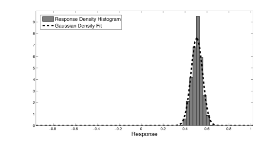
Figure 1: Histogram density of 300 oscillator models reinforced using the dynamics given in equations (21)–(23) for $y=0.5$. The histogram was obtained using 6300 points corresponding to 300 oscillators and 21 reinforcement trials per set of oscillators (trials 40 to 60). All parameters used were the same as those described in Suppes et al. (2012), and $K_{0}^{{}^{\prime}}$ was set to $4,500$. The fitted Gaussian has $\mu=0.51$ and $\sigma=0.05$, with $p<10^{-3}$.

shows the density histogram for a MATLAB simulation of the three oscillator model. Not surprisingly, the model’s smearing distribution $k_{s}(x|z)$ fits well a Gaussian

$$k_{s}\left(x|z\right)=\frac{1}{\sigma\sqrt{2\pi}}e^{-\frac{\left(x-z\right)^{2}}{2\sigma^{2}}},$$

where $\sigma=0.05$. We should mention that the estimation of the smearing distribution from a reinforcement schedule given by the Dirac delta function is not realistic for real psychological experiments. However, because we are running simulations without taking into consideration other behavioral and environmental aspects, we are able to extract $k_{s}(x|y)$ from it.

With the smearing distribution, we may now describe how a stochastic decision making processes may happen in the brain. Let $X$ and $Y$ be two of the possible responses for a certain behavioral experiment. In our model, response $X$ would be associated with an oscillator, $r_{1}\left(t\right)$, and $Y$ with the other, $r_{2}\left(t\right)$. If $I_{1}=2A^{2}$ and $I_{2}=0$, then the response would clearly be $I_{1}$. Since $-1\leq x\leq 1$, $x$ given by 16, we may state that $x>0$ corresponds to a response $X$ and $x\leq 0$ to response $Y$. If we do this, when the reinforcement is a value different from $1$ or $-1$, there is a nonzero chance, given by the smearing distribution, to select each response. In other words, say a stimulus $s_{a}$ is conditioned to $-1\leq z\leq 1$. Then,

$$P(X) = \int_{0}^{1}k_{s_{a}}\left(x|z\right)dx$$

$$\approx \frac{1}{2}+\frac{1}{2}\mbox{erf}\left(\frac{z}{\sqrt{2}\sigma}\right)$$

and

$$P(Y) = \int_{-1}^{0}k_{s_{a}}\left(x|z\right)dx$$

$$\approx \frac{1}{2}-\frac{1}{2}\mbox{erf}\left(\frac{z}{\sqrt{2}\sigma}\right),$$

for $\left|z\right|,\sigma\ll 1$, where $\mbox{erf}\left(x\right)$ is the error function. So, we can use the expression

$$z=\sqrt{2}\sigma\mbox{erf}^{-1}\left(2P\left(R_{1}\right)-1\right)$$

to estimate the reinforcement value $z$ leading to the desired probabilities of responses. Let us summarize the oscillator implementation of the Won/Lost version. We started with two stimulus, either Won or Lost, corresponding to the oscillators $s_{a}\left(t\right)$ and $s_{\overline{a}}\left(t\right)$. Once $s_{a}\left(t\right)$ or $s_{\overline{a}}\left(t\right)$ are activated, the dynamics of the system leads to a selection of either $X$ or $Y$, corresponding to the decisions of betting or not betting on the next step of the game.

We now model the “Disjunctive Version.” Because the response Win or Lost is not known, we assume that both oscillators $s_{a}\left(t\right)$ and $s_{\overline{a}}\left(t\right)$ are activated simultaneously. Furthermore, since the subject also knows that we either Win or we Lose, oscillators $s_{a}\left(t\right)$ and $s_{\overline{a}}\left(t\right)$ are incompatible, in the sense that they must represent off-phase oscillations in an SR-oscillator model. Therefore, the response system is composed not only of three oscillators, but four: the two stimulus and the two response oscillators. The equivalent dynamical expressions for (26)–(43) when both oscillators are activated are the following.

$$\dot{\varphi}_{s_{a}} = \omega_{0}-k_{s_{a},r_{1}}^{E}\sin\left(\varphi_{s_{a}}-\varphi_{r_{1}}\right)$$ (44)

$$-k_{s_{a},r_{2}}^{E}\sin\left(\varphi_{s_{a}}-\varphi_{r_{2}}\right)$$

$$-k_{s_{a},s_{\overline{a}}}^{I}\cos\left(\varphi_{s_{a}}-\varphi_{s_{\overline{a}}}\right)$$

$$-k_{s_{a},r_{1}}^{I}\cos\left(\varphi_{s_{a}}-\varphi_{r_{1}}\right)$$

$$-k_{s_{a},r_{2}}^{I}\cos\left(\varphi_{s_{a}}-\varphi_{r_{2}}\right),$$

$$\dot{\varphi}_{s_{\overline{a}}} = \omega_{0}-k_{s_{\overline{a}},r_{1}}^{E}\sin\left(\varphi_{s_{\overline{a}}}-\varphi_{r_{1}}\right)$$ (45)

$$-k_{s_{\overline{a}},r_{2}}^{E}\sin\left(\varphi_{s_{\overline{a}}}-\varphi_{r_{2}}\right)$$

$$-k_{s_{\overline{a}},s_{a}}^{I}\cos\left(\varphi_{s_{\overline{a}}}-\varphi_{s_{a}}\right)$$

$$-k_{s_{\overline{a}},r_{1}}^{I}\cos\left(\varphi_{s_{\overline{a}}}-\varphi_{r_{1}}\right)$$

$$-k_{s_{\overline{a}},r_{2}}^{I}\cos\left(\varphi_{s_{\overline{a}}}-\varphi_{r_{2}}\right),$$

$$\dot{\varphi}_{r_{1}} = \omega_{0}-k_{r_{1},s_{a}}^{E}\sin\left(\varphi_{r_{1}}-\varphi_{s_{a}}\right)$$ (46)

$$-k_{r_{1},s_{\overline{a}}}^{E}\sin\left(\varphi_{r_{1}}-\varphi_{s_{\overline{a}}}\right)$$

$$-k_{r_{1},r_{2}}^{E}\sin\left(\varphi_{r_{1}}-\varphi_{r_{2}}\right)$$

$$-k_{r_{1},s_{a}}^{I}\cos\left(\varphi_{r_{1}}-\varphi_{s_{a}}\right)$$

$$-k_{r_{1},s_{\overline{a}}}^{I}\cos\left(\varphi_{r_{1}}-\varphi_{s_{\overline{a}}}\right)$$

$$-k_{r_{1},r_{2}}^{I}\cos\left(\varphi_{r_{1}}-\varphi_{r_{2}}\right),$$

$$\dot{\varphi}_{r_{2}} = \omega_{0}-k_{r_{2},r_{1}}^{E}\sin\left(\varphi_{r_{2}}-\varphi_{r_{1}}\right)$$ (47)

$$-k_{r_{2},s_{a}}^{E}\sin\left(\varphi_{r_{2}}-\varphi_{s_{a}}\right)$$

$$-k_{r_{2},s_{\overline{a}}}^{E}\sin\left(\varphi_{r_{2}}-\varphi_{s_{\overline{a}}}\right)$$

$$-k_{r_{2},r_{1}}^{I}\cos\left(\varphi_{r_{2}}-\varphi_{r_{1}}\right)$$

$$-k_{r_{2},s_{a}}^{I}\cos\left(\varphi_{r_{2}}-\varphi_{s_{a}}\right)$$

$$-k_{r_{2},s_{\overline{a}}}^{I}\cos\left(\varphi_{r_{2}}-\varphi_{s_{\overline{a}}}\right),$$

with the couplings between $s_{a}$ and $r_{1}$ and $r_{2}$ as well as $s_{\overline{a}}$ and $r_{1}$ and $r_{2}$ being the same, but

$$k_{s_{a},s_{\overline{a}}}^{I}=\alpha^{\prime}.$$ (48)

As mentioned above, the parameter $\alpha^{\prime}$ in (48) represents a measure of the the degree of incompatibility of stimulus oscillators $s_{a}\left(t\right)$ and $s_{\overline{a}}\left(t\right)$.

Now, as above, let $I^{\prime}_{1}$ be the mean intensity at $r_{1}\left(t\right)$ given by

$$I^{\prime}_{1}=\left\langle\left(s_{a}(t)+s_{\overline{a}}\left(t\right)+r_{1}(t)\right)^{2}\right\rangle,$$

where this time we have both $s_{a}\left(t\right)$ and $s_{\overline{a}}\left(t\right)$ contributing to the intensity. Defining $\delta\varphi_{r_{1},a}\equiv\varphi_{r_{1}}-\varphi_{s_{a}}$ and $\delta\varphi_{r_{1},\overline{a}}\equiv\varphi_{r_{1}}-\varphi_{s_{\overline{a}}}$, it is straightforward to show that

$$I^{\prime}_{1} = A^{2}\left(\frac{3}{2}+\cos\left(\delta\varphi_{r_{1},a}\right)+\cos\left(\delta\varphi_{r_{1},\overline{a}}\right)+\cos\left(\delta\varphi_{r_{1},a}-\delta\varphi_{r_{1},\overline{a}}\right)\right).$$

Similarly, for $r_{2}\left(t\right)$ we have

$$I^{\prime}_{2} = A^{2}\left(\frac{3}{2}+\cos\left(\delta\varphi_{r_{2},a}\right)+\cos\left(\delta\varphi_{r_{2},\overline{a}}\right)+\cos\left(\delta\varphi_{r_{2},a}-\delta\varphi_{r_{2},\overline{a}}\right)\right).$$

We notice that, because we now have more oscillators, extra interference terms shows up in the intensity. We now use the new intensities, $I^{\prime}_{1}$ and $I^{\prime}_{2}$ to compute the response, using

$$b^{\prime}=\frac{I^{\prime}_{1}-I^{\prime}_{2}}{I^{\prime}_{1}+I^{\prime}_{2}}.$$

At this point, we should remark on the appearance of quantum-like effects. The model we are using, of interfering oscillators, carry some similarities with the famous two-slit experiment (Suppes and de Barros, 1994a). In the two-slit experiment, a quantum particle can go through two slits, and then hit a phosphorous screen, thus being detected. Since a particle is a localized object, going through one slit should mean no interaction with the other slit, and therefore we should expect to make no difference whether we keep the other slit closed or open. However, if we open both slits, we observe different probability patterns than if we close one of the slits. In other words, if we close one of the slits, and therefore know through which slit the particle went through, we get a probability of observing the particle in a certain region of the screen. If, on the other hand, we do not close one of the slits, we do not know through which slit it went, and when we do not know, the probability of detecting the particle changes. Formally, let $L$ be the proposition “went through the slit on the left because the slit on the right was closed,” $R=$“went through the slit on the right because the slit on the left was closed,” and $A=$“was observed at a certain region on the screen.” Then, it is possible to choose a region on the screen such that

$$P(A|R)>P\left(\neg A|R\right),$$

and

$$P(A|L)>P\left(\neg A|L\right),$$

i.e., such that there are more particles being detected on it than outside of it. However, because of quantum interference, if we do not close the slits, and do not know where they went, it is again possible to have an $A$ such that the above holds and

$$P\left(A\right)<P\left(\neg A\right).$$

This is the two slit formal equivalent of the violation of STP.

Now, let us go back to the oscillator model. For the the Win/Lost Version, a single stimulus oscillator is active at a time. Such oscillator produces a dynamics that leads to a certain balance between the responses $X$ and $Y$. This corresponds to one slit open, when there is no interference from the other slit. However, for the Disjunctive Version, both oscillators are active, and their activity interferes with each other, in a way similar to the interference from the two-slit experiment. The strength of interference, i.e. the degree of coherence between the two oscillators, is determined by the inhibitory coupling parameter $k_{s_{a},s_{\overline{a}}}^{I}$. Therefore, when both oscillators are active, we obtain a probability distribution violating the standard axioms of probability, and consequently STP.

To end this section, let us look at a simulation of the violation of the STP using neural oscillators. We simulated in Matlab R2012a the oscillators’ dynamics determined by equations (26)–(43) and (44)–(48) using the Dormand-Prince method. For simplicity, and without loss of generality, all oscillators were assumed to have the same frequency of $11$ Hz, as this would allow the use of the couplings given by (35)–(40) and (48) without having to invoke learning equations, as in (Suppes et al., 2012). For our system, the parameters utilized were the following: $\Delta t_{r}=0.2$ s, $\sigma_{\varphi}=\sqrt{\pi/4}$, $k_{s_{a},r_{1}}^{E}=-k_{s_{a},r_{2}}^{E}=k_{r_{1},s_{a}}^{E}=k_{r_{2},s_{a}}^{E}=-0.011$ Hz, $k_{r_{1},r_{2}}^{E}=k_{r_{2},r_{1}}^{E}=-11$ Hz, $k_{s_{\overline{a}},r_{1}}^{I}=-k_{s_{\overline{a}},r_{2}}^{I}=-k_{r_{1},s_{\overline{a}}}^{I}=k_{r_{2},s_{\overline{a}}}^{I}=1$, $k_{s_{\overline{a}},r_{1}}^{E}=-k_{s_{\overline{a}},r_{2}}^{E}=k_{r_{1},s_{\overline{a}}}^{E}=k_{r_{2},s_{\overline{a}}}^{E}=-0.017$ Hz, $k_{s_{\overline{a}},r_{1}}^{I}=-k_{s_{\overline{a}},r_{2}}^{I}=-k_{r_{1},s_{\overline{a}}}^{I}=k_{r_{2},s_{\overline{a}}}^{I}=1$, $k_{r_{1},r_{2}}^{I}=k_{r_{2},r_{1}}^{I}=0$, and $k_{s_{a},s_{\overline{a}}}^{I}=k_{s_{\overline{a}},s_{a}}^{I}=-0.011$, where $\Delta t_{r}$ is the time of response after the onset of stimulus, and $\sigma_{\varphi}$ is the variance of the initial conditions for the phase oscillators. We ran 1,000 trials with the above parameter values, for the Win/Lost Version we obtained $X$ as response 63% when the Lost oscillator was used and 58% with the Win oscillator. However, for the Disjunctive Version, when the two oscillators were active, we obtained $X$ as a response 36% of the runs, clearly showing a violation of Savage’s STP and an interference effect, as expected.

4 Conclusions

In this paper we presented a neural oscillator model based on reasonable assumptions about the behavior of coupled neurons. We then showed that the predictions of such model presents interference effects between incompatible stimulus oscillators. Such interference leads to computation of responses which are inconsistent with standard probability laws, but are consistent with quantum-like effects in decision making processes Busemeyer et al. (2009). Of course, the fact that we get interference from $s_{1}$ and $s_{2}$ does not preclude us from necessarily making rational decisions. We could, for example, modify the above model, and include an extra oscillator, such that after reinforcement we could eliminate interference, therefore satisfying the STP. But our model suggests that a plausible mechanism for quantum effects in the brain may not need to rely on actual quantum processes, as advocated by Penrose (1989), but instead can be a consequence of neuronal “interference.”

One interesting feature of the oscillator model is that the amount of interference between the oscillators is determined by the couplings between $s_{1}$ and $s_{2}$. The stronger the incompatibility between the two stimulus, the more we should see interference between the responses. Furthermore, because interference is a consequence of inhibitory couplings, we could in principle design experiments where pharmacological interventions could suppress inhibitory synapses, destroying such interference effects.

An attentive reader may question the possibility of modeling decision-making processes from neurons. In particular, how can we account for what Pattee claims are non-holonomic constraints not internalized by the dynamics (Pattee, 1972, 2001, 2012). To address this issue, let us examine this claim in more detail. First, we should notice that there are many examples of non-holonomic constraints in physical systems that are determined by an underlying and well-understood dynamics. For example, a ball rolling without slipping on a flat surface satisfies such type of constraint. But most physicists would not think that such an example presents fundamental difficulties to the description of the system ball-surface. In this case, what is a constraint and what is a physical system is just a matter of computational convenience. As a trained physicists himself, we believe this is not what Pattee meant.

For Pattee, decision making processes require the type of discontinuous jump that cannot be associated to classical dynamical systems, but can be thought of as determined by non-holonomic constraints in a classical dynamics. Since the fundamental laws of physics do not have such characteristics, he reasons, it remains a mystery how they emerge from complex systems. He goes on to propose that the jumps come from the emergence of quantum decoherence (using the modern parlance).

Going back to the model presented here, the question remains on how we can derive such emergent characteristics. First, we emphasize that we are not modeling decision making processes from basic physics, but instead from emerging properties of collections of neurons. In other words, we are assuming an emerging dynamics with the necessary features described by Pattee (1972): nonlinearity and time-dependent dynamics (Guckenheimer and Holmes, 1983). For instance, overall dynamics of a highly complex system of interacting neurons is modeled mathematically with nonlinear equations describing the behavior of phases (which adds to the nonlinearity). Furthermore, the decision-making dynamics changes in time by reinforcements which are outside of the dynamical system itself (Suppes et al., 2012). Such reinforcements are not only time-dependent, but can also be viewed as non-holonomic constraints to the dynamics. Thus, in a certain sense, we are not addressing the fundamental problem posed by Pattee, but we do push it to another level in the description of neural interactions.

It is also important to clarify the relationship between our model and quantum mechanics. We are not claiming that we derive quantum mechanics from neuronal dynamics. We are showing that certain quantum-like features (but not all; see de Barros and Suppes, 2009, for details) are present in our model. In other words, we start with a classical stochastic description and obtain some quantum-like results. This is to be contrasted with Pattee, who argues that classical-like dynamics emerges from a quantum world, and such emergence happens with the appearance of life itself.

We end this paper with a comparison between our model and the one proposed by Khrennikov (2011). Whereas in Khrennikov’s model the interference of electromagnetic fields account for quantum-like effects in the brain, in our model we use Kuramoto oscillators to describe the evolution of coupled sets of dynamical oscillators close to Andronov-Hopf bifurcations. Because such oscillators obey a wave equation, they are subject to interference. So, in some sense, we may say that the oscillator and the field models are equivalent representations of quantum-like interference in the brain. However, though we can think of the weak couplings between oscillators originating from the synapses between neurons, it is also conceivable that the weak oscillating electric fields generated by sets of oscillators provide sufficient additional coupling to account for their synchronization and interference. Thus, we believe that there are not only equivalencies between the models, but also that our oscillator model might provide an underlying neurophysiological justification for Khrennikov’s quantum-like field processing. It would be interesting to prove some representation theorem between neural oscillators and Khrennikov’s field model. However, this seems implausible, since it was shown in de Barros (2012) that oscillators may generate processes that are not representable in terms of observables in a Hilbert space, and Khrennikov’s model relies on a quantum representation of states in terms of Hilbert spaces.

Acknowledgments

The author wishes to thank Dr. Gary Oas for critical reading and discussion on the contents of this manuscript, as well as the anonymous referee for useful comments and suggestions.

References

- Aerts (2009) Aerts, D., 2009. Quantum structure in cognition. Journal of Mathematical Psychology 53, 314–348.
- Asano et al. (2010) Asano, M., Ohya, M., Khrennikov, A., 2010. Quantum-like model for decision making process in two players game. Foundations of Physics 41, 538–548.
- Baaquie (1997) Baaquie, B.E., 1997. A path integral approach to option pricing with stochastic volatility: Some exact results. Journal de Physique I 7, 1733–1753.
- de Barros (2011) de Barros, J.A., 2011. Comments on “There is no axiomatic system for the quantum theory”. International Journal of Theoretical Physics 50, 1828–1830.
- de Barros (2012) de Barros, J.A., 2012. Joint probabilities and quantum cognition, in: Khrennikov, A. (Ed.), Proceedings of Quantum Theory: Reconsiderations of Foundations - 6, Institute of Physics, Växjö, Sweden. To appear.
- de Barros et al. (2007) de Barros, J.A., de Mendonça, J.P.R.F., Pinto-Neto, N., 2007. Realism in energy transition processes: an example from Bohmian quantum mechanics. Synthese 154, 349–370.
- de Barros et al. (2012) de Barros, J.A., Oas, G., Suppes, P., 2012. Response selection using neural phase oscillators. arXiv:1208.6041 Submitted to the Festschrift in Honor of Patrick Suppes’s 90th Birthday.
- de Barros and Suppes (2000) de Barros, J.A., Suppes, P., 2000. Inequalities for dealing with detector inefficiencies in Greenberger-Horne-Zeilinger type experiments. Physical Review Letters 84, 793–797.
- de Barros and Suppes (2001) de Barros, J.A., Suppes, P., 2001. Probabilistic results for six detectors in a three-particle GHZ experiment, in: Bricmont, J., Dürr, D., Galavotti, M.C., Ghirardi, G., Petruccione, F., Zanghi, N. (Eds.), Chance in Physics, p. 213.
- de Barros and Suppes (2009) de Barros, J.A., Suppes, P., 2009. Quantum mechanics, interference, and the brain. Journal of Mathematical Psychology 53, 306–313.
- de Barros and Suppes (2010) de Barros, J.A., Suppes, P., 2010. Probabilistic inequalities and upper probabilities in quantum mechanical entanglement. Manuscrito 33, 55–71.
- Bell (1964) Bell, J.S., 1964. On the Einstein-Podolsky-Rosen paradox. Physics 1, 195–200.
- Bell (1966) Bell, J.S., 1966. On the problem of hidden variables in quantum mechanics. Rev. Mod. Phys. 38, 447–452.
- Billock and Tsou (2005) Billock, V.A., Tsou, B.H., 2005. Sensory recoding via neural synchronization: integrating hue and luminance into chromatic brightness and saturation. J. Opt. Soc. Am. A 22, 2289–2298.
- Billock and Tsou (2011) Billock, V.A., Tsou, B.H., 2011. To honor Fechner and obey Stevens: relationships between psychophysical and neural nonlinearities. Psychological Bulletin 137, 1–18.
- Bruza et al. (2009) Bruza, P., Busemeyer, J.R., Gabora, L., 2009. Introduction to the special issue on quantum cognition. Journal of Mathematical Psychology 53, 303–305.
- Busemeyer and Wang (2007) Busemeyer, J., Wang, Z., 2007. Quantum information processing explanation for interactions between inferences and decisions, in: Proceedings of the Quantum Interaction Symposium AAAI Press, AAAI Press, Menlo Park, CA. pp. 91–97.
- Busemeyer et al. (2009) Busemeyer, J., Wang, Z., Lambert-Mogiliansky, A., 2009. Empirical comparison of markov and quantum models of decision making. Journal of Mathematical Psychology 53, 423–433.
- Busemeyer and Diederich (2010) Busemeyer, J.R., Diederich, A., 2010. Cognitive modeling. SAGE.
- Busemeyer et al. (2006) Busemeyer, J.R., Wang, Z., Townsend, J.T., 2006. Quantum dynamics of human decision-making. Journal of Mathematical Psychology 50, 220–241.
- Ford (1983) Ford, J., 1983. How random is a coin toss? Physics Today 36, 40.
- Galavotti (2005) Galavotti, M.C., 2005. Philosophical introduction to probability. volume 167 of CSLI Lecture Notes. CSLI Publications, Stanford, CA.
- Guckenheimer and Holmes (1983) Guckenheimer, J., Holmes, P., 1983. Nonlinear oscillations, dynamical systems, and bifurcations of vector fields. volume 42. Springer-Verlag New York.
- Haven (2002) Haven, E., 2002. A discussion on embedding the Black–Scholes option pricing model in a quantum physics setting. Physica A: Statistical Mechanics and its Applications 304, 507–524.
- Hoppensteadt and Izhikevich (1996a) Hoppensteadt, F.C., Izhikevich, E.M., 1996a. Synaptic organizations and dynamical properties of weakly connected neural oscillators i. analysis of a canonical model. Biological Cybernetics 75, 117–127.
- Hoppensteadt and Izhikevich (1996b) Hoppensteadt, F.C., Izhikevich, E.M., 1996b. Synaptic organizations and dynamical properties of weakly connected neural oscillators II. learning phase information. Biological Cybernetics 75, 129–135.
- Izhikevich (2007) Izhikevich, E.M., 2007. Dynamical Systems in Neuroscience: The Geometry of Excitability and Bursting. The MIT Press, Cambridge, Massachusetts.
- Jaynes (2003) Jaynes, E.T., 2003. Probability theory: the logic of science. Cambridge Univ Press, Cambridge, Great Britain.
- Josić et al. (2009) Josić, K., Rubin, J., Matias, M., 2009. Coherent Behavior in Neuronal Networks. Springer Verlag, Dordrecht, Holland.
- Khrennikov (2009) Khrennikov, A., 2009. Quantum-like model of cognitive decision making and information processing. Biosystems 95, 179–187.
- Khrennikov (2010) Khrennikov, A., 2010. Ubiquitous Quantum Structure. Springer Verlag, Heidelberg.
- Khrennikov (2011) Khrennikov, A., 2011. Quantum-like model of processing of information in the brain based on classical electromagnetic field. Biosystems 105, 250–262.
- Khrennikov and Haven (2009) Khrennikov, A., Haven, E., 2009. Quantum mechanics and violations of the sure-thing principle: The use of probability interference and other concepts. Journal of Mathematical Psychology 53, 378–388.
- Kochen and Specker (1975) Kochen, S., Specker, E.P., 1975. The problem of hidden variables in quantum mechanics, in: Hooker, C.A. (Ed.), The Logico-Algebraic Approach to Quantum Mechanics. D. Reidel Publishing Co., Dordrecht, Holland, p. 293–328.
- Kuramoto (1984) Kuramoto, Y., 1984. Chemical Oscillations, Waves, and Turbulence. Dover Publications, Inc., Mineola, New York.
- Mackintosh (1983) Mackintosh, N.J., 1983. Conditioning and associative learning. Clarendon Press Oxford.
- Nelson et al. (2003) Nelson, D.L., McEvoy, C.L., Pointer, L., 2003. Spreading activation or spooky action at a distance? Journal of Experimental Psychology: Learning, Memory, and Cognition 29, 42–51.
- von Neumann (1996) von Neumann, J., 1996. Mathematical Foundations of Quantum Mechanics. Princeton University Press, Princeton, NJ.
- Nunez and Srinivasan (2006) Nunez, P., Srinivasan, R., 2006. Electric Fields of the Brain: The Neurophysics of EEG, 2nd Ed. Oxford University Press, New York, NY. 2nd edition.
- Pattee (2012) Pattee, H., 2012. Epistemic, evolutionary, and physical conditions for biological information. Biosemiotics , 1–23.
- Pattee (1972) Pattee, H.H., 1972. Physical problems of decision-making constraints. International Journal of Neuroscience 3, 99–105.
- Pattee (2001) Pattee, H.H., 2001. The physics of symbols: bridging the epistemic cut. Biosystems 60, 5–21.
- Penrose (1989) Penrose, R., 1989. Emperor’s New Mind. Oxford University Press, New York, NY.
- Savage (1972) Savage, L.J., 1972. The foundations of statistics. Dover Publications Inc., Mineola, New York. 2nd edition.
- Seliger et al. (2002) Seliger, P., Young, S.C., Tsimring, L.S., 2002. Plasticity and learning in a network of coupled phase oscillators. Physical Review E 65, 041906–1–7.
- Shafir and Tversky (1992) Shafir, E., Tversky, A., 1992. Thinking through uncertainty: Nonconsequential reasoning and choice. Cognitive Psychology 24, 449–474.
- Suppes (1959) Suppes, P., 1959. A linear learning model for a continuum of responses, in: Bush, R.R., Estes, W.K. (Eds.), Studies in Mathematical Leaning Theory. Stanford University Press, Stanford, CA, pp. 400–414.
- Suppes (1970) Suppes, P., 1970. A probabilistic theory of causality. volume 24 of Acta Philosophica Fennica. North-Holland Publishing Company, Amsterdam, Holland.
- Suppes (2002) Suppes, P., 2002. Representation and Invariance of Scientific Structures. CSLI Publications, Stanford, California.
- Suppes and Atkinson (1960) Suppes, P., Atkinson, R.C., 1960. Markov learning models for multiperson interactions. Stanford University Press, Stanford, California.
- Suppes and de Barros (1994a) Suppes, P., de Barros, J.A., 1994a. Diffraction with well-defined photon trajectories: A foundational analysis. Foundations of Physics Letters 7, 501–514.
- Suppes and de Barros (1994b) Suppes, P., de Barros, J.A., 1994b. A random-walk approach to interference. International Journal of Theoretical Physics 33, 179–189.
- Suppes and de Barros (1996) Suppes, P., de Barros, J.A., 1996. Photons, billiards and chaos, in: Weingartner, P., Schurz, G. (Eds.), Law and Prediction in the Light of Chaos Research. Springer Berlin Heidelberg. volume 473, pp. 189–201.
- Suppes and de Barros (2007) Suppes, P., de Barros, J.A., 2007. Quantum mechanics and the brain, in: Quantum Interaction: Papers from the AAAI Spring Symposium, AAAI Press, Menlo Park, CA. p. 75–82.
- Suppes et al. (1996a) Suppes, P., de Barros, J.A., Oas, G., 1996a. A collection of probabilistic hidden-variable theorems and counterexamples, in: Pratesi, R., Ronchi, L. (Eds.), Waves, Information, and Foundations of Physics: a tribute to Giuliano Toraldo di Francia on his 80th birthday, Italian Physical Society, Florence, Italy.
- Suppes et al. (2012) Suppes, P., de Barros, J.A., Oas, G., 2012. Phase-oscillator computations as neural models of stimulus–response conditioning and response selection. Journal of Mathematical Psychology 56, 95–117.
- Suppes et al. (1996b) Suppes, P., de Barros, J.A., Sant’Anna, A.S., 1996b. A proposed experiment showing that classical fields can violate bell’s inequalities. arXiv:quant-ph/9606019 .
- Suppes et al. (1996c) Suppes, P., de Barros, J.A., Sant’Anna, A.S., 1996c. Violation of bell’s inequalities with a local theory of photons. Foundations of Physics Letters 9, 551–560.
- Suppes et al. (1996d) Suppes, P., Sant’Anna, A., Barros, J., 1996d. A particle theory of the casimir effect. Foundations of Physics Letters 9, 213–223.
- Suppes and Zanotti (1981) Suppes, P., Zanotti, M., 1981. When are probabilistic explanations possible? Synthese 48, 191–199.
- Trevisan et al. (2005) Trevisan, M.A., Bouzat, S., Samengo, I., Mindlin, G.B., 2005. Dynamics of learning in coupled oscillators tutored with delayed reinforcements. Physical Review E 72, 011907.
- Tversky and Shafir (1992) Tversky, A., Shafir, E., 1992. The disjunction effect in choice under uncertainty. Psychological Science 3, 305–309.
- Vassilieva et al. (2011) Vassilieva, E., Pinto, G., de Barros, J.A., Suppes, P., 2011. Learning pattern recognition through quasi-synchronization of phase oscillators. IEEE Transactions on Neural Networks 22, 84–95.
- Vulović and Prange (1986) Vulović, V.Z., Prange, R.E., 1986. Randomness of a true coin toss. Physical Review A 33, 576–582.
- Werndl (2009) Werndl, C., 2009. Are deterministic descriptions and indeterministic descriptions observationally equivalent? Studies in history and philosophy of science part B: studies in history and philosophy of modern physics 40, 232–242.