Analysis of astrometric catalogues with vector spherical harmonics

Abstract

Aims. We compare stellar catalogues with position and proper motion components using a decomposition on a set of orthogonal vector spherical harmonics. We aim to show the theoretical and practical advantages of this technique as a result of invariance properties and the independence of the decomposition from a prior model.

Methods. We describe the mathematical principles used to perform the spectral decomposition, evaluate the level of significance of the multipolar components, and examine the transformation properties under space rotation.

Results. The principles are illustrated with a characterisation of systematic effects in the FK5 catalogue compared to Hipparcos and with an application to extraction of the rotation and dipole acceleration in the astrometric solution of QSOs expected from Gaia.

1 Introduction

The differences between the positions of a set of common sources in two astrometric catalogues are conveniently described mathematically by a vector field on a sphere. Each vector materialises the difference between the two unit vectors giving the direction of the common sources in each catalogue. This feature extends to the differences between the proper motions of each source which also generates a spherical vector field. Typically when connecting two positional catalogues with $n$ common sources, one has the coordinates $\alpha_{i}^{(1)},\delta_{i}^{(1)}$ for the $i$th source in the first catalogue and $\alpha_{i}^{(2)},\delta_{i}^{(2)}$ for the same source in the second catalogue. Provided the two catalogues are close to each other, the differences can be mapped as a vector field with components in the local tangent plane given by

$$\mbox{\boldmath$V$}=[\Delta\alpha\cos\delta=(\alpha^{(2)}-\alpha^{(1)})\cos\delta^{(1)},\ \Delta\delta=\delta^{(2)}-\delta^{(1)}]$$ (1)

for each common source between the two catalogues. We wish to analyse these fields in order to summarise their largest overall or local features by means of a small set of base functions, which is much smaller in any case than the number of sources.

Several papers in the astronomical literature have applied this overall idea with either scalar or vectorial functions. As far as we have been able to trace the relevant publications regarding the use of vector spherical harmonics in this context, this has been initiated by Mignard & Morando (1990) and published in a proceedings paper that is not widely accessible. One of the motivations of this paper is therefore to update and expand on this earlier publication and to provide more technical details on the methodology.

The general idea of the decomposition has its root in the classical expansion of a scalar function defined on the unit sphere with a set of mutually orthogonal spherical harmonics functions. The most common case in astronomy and geodesy is the expansion of the gravitational potential of celestial bodies, in particular that of the Earth. The generalisation of such expansions to vectors, tensors, or even arbitrary fields was introduced in mathematics and theoretical physics decades ago (Gelfand, Minlos & Shapiro 1963). For example, these generalisations are widely used in gravitational physics (Throne 1980; Suen 1986; Blanchet & Damour 1986). Restricting it to the case of vectors fields, which is the primary purpose of this paper, we look for a set of base functions that would allow representing any vector field on the unit sphere as an infinite sum of fields, so that the angular resolution would increase with the degree of the representation (smaller details being described by the higher harmonics). One would obviously like for the lowest degrees to represent the most conspicuous features seen in the field, such as a rotation about any axis or systematic distortion on a large scale. It is important to stress at this point that expanding a vector field on this basis function is not at all the same as expanding the two scalar fields formed by the components of the vector field: the latter would depend very much on the coordinate system used, while a direct representation on a vectorial basis function reveals the true geometric properties of the field, regardless of the coordinate system, in the same way as the vector field can be plotted on the sphere without reference to a particular frame without a graticule drawn in the background.

Several related methods using spherical functions to model the errors in astrometric catalogues, the angular distribution of proper motions, or more simply as a means of isolating a rotation have been published and sometimes with powerful algorithms. Brosche (1966, 1970) was probably the first to suggest the use of orthogonal functions to characterise the errors in all-sky astrometric catalogue, and his method was later improved by Schwan (1977) to allow for a magnitude dependence. But in both cases the analysis was carried out separately for each component $\Delta\alpha\cos\delta,\Delta\delta$ of the error, by expanding two scalar functions. Therefore, this was not strictly an analysis of a vector field, but that of its components on a particular reference frame. The results therefore did not describe the intrinsic geometric properties of the field, which should reveal properties not connected to a particular frame (see also Appendix C). Similarly, a powerful method for exhibiting primarily the rotation has been developed in a series of papers of Vityazev (2010, and references therein). The vector spherical harmonics (hereafter abridged in VSH) have been in particular used in several analyses of systematic effects in VLBI catalogues or in comparison of reference frames, such as in Arias et al. (2000), Titov & Malkin (2009), or Gwinn et al. (1997), the galactic velocity field (Makarov & Murphy 2007), the analysis of zonal errors in space astrometry (Makarov et al. 2012), but none of these papers deals with the fundamental principles, the very valuable invariance properties and the relevant numerical methods. Within the Gaia preparatory activities the VSH are used also to compare sphere solutions and in the search of systematic differences at different scales by Bucciarelli et al (2011) and more is planned in the future to characterise and evaluate the global astrometric solution.

In this paper we provide the necessary theoretical background to introduce the VSHs and the practical formulas needed to explicitly compute the expansion of a vector field. The mathematical principles are given in Section 2 with a few illustrations to show the harmonics of lower degrees. In the next section, Section 3, we emphasise the transformation of the VSHs and that of the expansion of a vector field under a rotation of the reference frame, with applications to the most common astronomical frames. Then in Section 4 we discuss the physical interpretation of the harmonics of first degree as the way of representing the global effect shown by a vector field, such as the axial rotation and its orthogonal counterpart, for which we have coined the term glide, and show its relationship to the dipole axial acceleration resulting from the Galactic aberration. The practical implementation is taken up in Section 5, where we also discuss the statistical testing of the power found in each harmonic. The results of particular applications to the FK5 Catalogue and to the simulated QSO catalogue expected from Gaia are respectively given in Sects.  6 and 7. Appendix A provides the explicit expressions of the VSH up to degree $l=4$, while Appendix B deals with the practical formulas needed for numerical evaluation of the VSH, and Appendix C focuses on the relationship between expansions of the components of a vector field on the scalar spherical harmonics and the expansion of the same field on the VSHs.

2 Mathematical principles

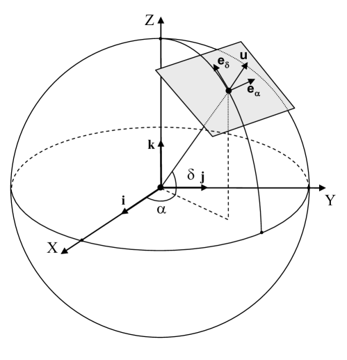
Figure 1: Local frame associated to the spherical coordinates $\alpha,\delta$, with the unit vectors along the longitude and latitude lines.

2.1 Definitions

In this section we give the main definitions needed to use the VSHs and the theoretical background from which practical numerical methods are established and discussed later in the paper. The VSHs form an orthogonal set of basis functions for a vector field on a sphere and split into two categories referred to as the toroidal $\mbox{\boldmath$T$}_{lm}$ and spheroidal $\mbox{\boldmath$S$}_{lm}$ functions (in the physical literature the former are also called “magnetic” or “stream”, and the latter “poloidal”, “potential”, or “electric”):

$$\mbox{\boldmath$S$}_{lm} = \frac{1}{\sqrt{l(l+1)}}\,r\,\mbox{\boldmath$\nabla$}Y_{lm}=\mbox{\boldmath$u$}\times\mbox{\boldmath$T$}_{lm}\,,$$ (2)

$$\mbox{\boldmath$T$}_{lm} = -\,\mbox{\boldmath$u$}\times\mbox{\boldmath$S$}_{lm}\,,$$ (3)

where $\mbox{\boldmath$u$}=\mbox{\boldmath$r$}/r$, $r=|\mbox{\boldmath$r$}|$, $r$ is the radius-vector of the point, and $\nabla$ denotes the gradient operator. Clearly, for points on the surface of a unit sphere $r=1$. It is also obvious that at each point on the sphere and for each $l$ and $m$ one has $\mbox{\boldmath$u$}\cdot\mbox{\boldmath$S$}_{lm}=0$, $\mbox{\boldmath$u$}\cdot\mbox{\boldmath$T$}_{lm}=0$, and $\mbox{\boldmath$T$}_{lm}\cdot\mbox{\boldmath$S$}_{lm}=0$. Taking into account that (see Fig. 1)

$$u = \pmatrix{\cos\alpha\,\cos\delta\cr\sin\alpha\,\cos\delta\cr\sin\delta}\,,$$ (4)

$$\mbox{\boldmath$e$}_{\alpha} = {1\over\cos\delta}\,{\partial\over\partial\alpha}\mbox{\boldmath$u$}=\pmatrix{-\sin\alpha\cr\phantom{-}\cos\alpha\cr 0}\,,$$ (5)

$$\mbox{\boldmath$e$}_{\delta} = \mbox{\boldmath$u$}\times\mbox{\boldmath$e$}_{\alpha}={\partial\over\partial\delta}\,\mbox{\boldmath$u$}=\pmatrix{-\cos\alpha\,\sin\delta\,\cr-\sin\alpha\,\sin\delta\cr\cos\delta},$$ (6)

(so that $|\mbox{\boldmath$u$}|=1$, $|\mbox{\boldmath$e$}_{\alpha}|=1$, $|\mbox{\boldmath$e$}_{\delta}|=1$), one gets explicit formulas

$$\mbox{\boldmath$T$}_{lm}(\alpha,\delta)=\frac{1}{\sqrt{l(l+1)}}\left[\frac{\partial Y_{lm}}{\partial\delta}\mbox{\boldmath$e$}_{\alpha}-\frac{1}{\cos\delta}\frac{\partial Y_{lm}}{\partial\alpha}\mbox{\boldmath$e$}_{\delta}\right]$$ (7)

for the toroidal functions, and

$$\mbox{\boldmath$S$}_{lm}(\alpha,\delta)=\frac{1}{\sqrt{l(l+1)}}\left[\frac{1}{\cos\delta}\frac{\partial Y_{lm}}{\partial\alpha}\mbox{\boldmath$e$}_{\alpha}+\frac{\partial Y_{lm}}{\partial\delta}\mbox{\boldmath$e$}_{\delta}\right]$$ (8)

for the spheroidal functions. The $Y_{lm}$ are the standard spherical functions defined here with the following sign convention

$$Y_{lm}(\alpha,\delta)=(-1)^{m}\,\sqrt{\frac{2l+1}{4\pi}\,\frac{(l-m)!}{(l+m)!}}\,P_{lm}(\sin\delta)\,e^{\buildrel\circ\over{\i}m\alpha}$$ (9)

for $m\geq 0$ and

$$Y_{l,-m}(\alpha,\delta)=(-1)^{m}\,Y_{lm}^{\ast}(\alpha,\delta)$$ (10)

for $m<0$, where superscript ‘$\ast$’ denotes complex conjugation. The associated Legendre functions are defined as

$$P_{lm}(x)=(1-x^{2})^{m/2}\,\frac{d^{m}P_{l}(x)}{dx^{m}}.$$ (11)

Equations (9)–(10) agree with the well-known formula for the associated Legendre functions

$$P_{l,-m}(x)=(-1)^{m}\,{(l-m)!\over(l+m)!}\,P_{lm}(x)\,.$$ (12)

Different sign conventions appear in the literature, in particular regarding the place of the $(-1)^{m}$, which is sometimes used in the definition of the associated Legendre functions instead (see, e.g., Chapter 8 of Abramowitz & Stegun 1972). However, these sign differences do not influence the vector spherical functions themselves. Also one sometimes considers $\buildrel\circ\over{\i}\,\mbox{\boldmath$T$}_{lm}$ instead of $\mbox{\boldmath$T$}_{lm}$ as the toroidal vector spherical functions.

From (10) and (7)–(8) one immediately has

$$\mbox{\boldmath$T$}_{l,-m}(\alpha,\delta) = (-1)^{m}\,\mbox{\boldmath$T$}_{lm}^{\ast}(\alpha,\delta)\,,$$ (13)

$$\mbox{\boldmath$S$}_{l,-m}(\alpha,\delta) = (-1)^{m}\,\mbox{\boldmath$S$}_{lm}^{\ast}(\alpha,\delta)\,.$$ (14)

2.2 Orthogonality properties

The spherical functions $Y_{lm}$ form an orthonormal sequence of functions on the surface of a sphere since

$$\int_{\Omega}\,Y_{lm}Y_{l^{\prime}m^{\prime}}^{\ast}\,d\Omega=\delta^{ll^{\prime}}\delta^{mm^{\prime}}\,,$$ (15)

which is also complete in the Hilbert space $\mathcal{S}$ of the square-integrable functions on a sphere (making it an orthonormal basis of $\mathcal{S}$ in the $L^{2}$ norm). As in Fourier expansions, the completeness property is hard to establish and is related to the fact that spherical harmonics are eigenfunctions of a special kind of differential equations (see, for example, Morse & Feshbach 1954). This is accepted and not further discussed in this paper directed towards astronomical applications. Here and below one has $d\Omega=\cos\delta\,d\delta\,d\alpha$, and the integration is taken over the surface of the unit sphere: $0\leq\alpha\leq 2\pi$, $-\pi/2\leq\delta\leq\pi/2$, and $\delta^{ij}$ is the Kronecker symbol: $\delta^{ij}=1$ for $i=j$ and $\delta^{ij}=0$, otherwise.

Thanks to the completeness property a (square-integrable) complex-valued scalar function defined on a unit sphere $f(\alpha,\delta)$ can be uniquely projected on the $Y_{lm}$:

$$f(\alpha,\delta)=\sum_{l=0}^{\infty}\sum_{m=-l}^{l}f_{lm}\,Y_{lm}\,,$$ (16)

where the Fourier coefficients $f_{lm}$ age given by

$$f_{lm}=\int_{\Omega}\,f\,Y^{\ast}_{lm}\,d\Omega\,.$$ (17)

The equality in (16) strictly means that the right-hand side series converge (not necessarily pointwise at discontinuity points or singularities but at least with the $L^{2}$ norm) to some function $f$, and given the completeness and the orthonormal basis, the coefficients $f_{lm}$ are related to $f$ by (17). A truncated form of (16) with $l\leq l_{\mathrm{max}}<\infty$ is an approximate expansion for which the equality in (16) does not strictly hold (in general).

Similarly, the VSH form a complete set of orthonormal vector functions on the surface of a sphere (with the inner product of the $L^{2}$ space):

$$\int_{\Omega}\,\mbox{\boldmath$T$}_{lm}\cdot\mbox{\boldmath$T$}^{\ast}_{l^{\prime}m^{\prime}}\,d\Omega=\delta^{ll^{\prime}}\delta^{mm^{\prime}}\,,$$ (18)

$$\int_{\Omega}\,\mbox{\boldmath$S$}_{lm}\cdot\mbox{\boldmath$S$}^{\ast}_{l^{\prime}m^{\prime}}\,d\Omega=\delta^{ll^{\prime}}\delta^{mm^{\prime}}\,,$$ (19)

$$\int_{\Omega}\,\mbox{\boldmath$S$}_{lm}\cdot\mbox{\boldmath$T$}^{\ast}_{l^{\prime}m^{\prime}}\,d\Omega=0\,.$$ (20)

As we noted after (3) above, one also has the orthogonality between two vectors in the usual Euclidean space,

$$\mbox{\boldmath$S$}_{lm}\cdot\mbox{\boldmath$T$}_{lm}=0$$ (21)

which holds for any point on the sphere.

Any (square-integrable) complex-valued vector field $\mbox{\boldmath$V$}(\alpha,\delta)$ defined on the surface of a sphere and orthogonal to $u$ (radial direction),

$$\mbox{\boldmath$V$}(\alpha,\delta)=V^{\alpha}(\alpha,\delta)\,\mbox{\boldmath$e$}_{\alpha}+V^{\delta}(\alpha,\delta)\,\mbox{\boldmath$e$}_{\delta}\,,$$ (22)

can be expanded in a unique linear combination of the VSH,

$$\mbox{\boldmath$V$}(\alpha,\delta)=\sum_{l=1}^{\infty}\,\sum_{m=-l}^{l}\,\bigl{(}t_{lm}\mbox{\boldmath$T$}_{lm}+s_{lm}\mbox{\boldmath$S$}_{lm}\bigr{)}\,,$$ (23)

where the coefficients $t_{lm}$ and $s_{lm}$ can again be computed by projecting the field on the base functions with

$$t_{lm} = \int_{\Omega}\,\mbox{\boldmath$V$}\cdot\mbox{\boldmath$T$}^{\ast}_{lm}\,d\Omega\,,$$ (24)

$$s_{lm} = \int_{\Omega}\,\mbox{\boldmath$V$}\cdot\mbox{\boldmath$S$}^{\ast}_{lm}\,d\Omega\,.$$ (25)

2.3 Numerical computation of the vector spherical harmonics

Analytical expressions of the VSH are useful for the lower orders to better understand what fields are represented with large-scale features and also to experiment by hand on simple fields in an analytical form. This helps develop insight into their properties and behaviour, which pays off at higher orders when one must rely only on numerical approaches. This is also a good way to test a computer implementation by comparing the numerical output to the expected results derived from the analytical expressions. Analytical expressions for the vector spherical harmonics of orders $l\leq 4$ are given explicitly as a function of $\alpha$ and $\delta$ in Appendix A.

To go to higher degrees, one needs to resort to numerical methods. To numerically compute the two components of $\mbox{\boldmath$T$}_{lm}(\alpha,\delta)$ and $\mbox{\boldmath$S$}_{lm}(\alpha,\delta)$ given by (7)–(8), one first needs to have a procedure for the scalar spherical harmonics. Given the form of the $Y_{lm}(\alpha,\delta)$ in (9), the derivative with respect to $\alpha$ is trivial, and for $\delta$ only, the derivative of the Legendre associated functions needs special care. There are several recurrence relations allowing the Legendre functions to be computed, but not all of them are stable for high degrees. Other difficulties appear around the poles when $\delta\pm\pi/2$ where care must be exercised to avoid singularities. Non-singular expressions and numerically stable algorithms for computing the VSH components are available in the literature, and the expressions we have implemented and tested are detailed in Appendix B.

2.4 Expansions of real functions

Describing real-valued vector fields with complex-valued VSHs leads to unnecessary redundancy in the number of basis functions and fitting coefficients. In general, the coefficients in (23) are complex even for a real vector field. But for a real field $\mbox{\boldmath$V$}(\alpha,\delta)$, the expansion must be real. Given the conjugation properties of the VSH, it is clear that for a real-values function one gets

$$t_{lm} = (-1)^{m}\,t^{\ast}_{l,-m}\,,$$ (26)

$$s_{lm} = (-1)^{m}\,s^{\ast}_{l,-m}\,.$$ (27)

Then from the decomposition of the coefficients into their real and imaginary parts as

$$t_{lm} = t^{\Re}_{lm}+\buildrel\circ\over{\i}\,t^{\Im}_{lm}\,,$$ (28)

$$s_{lm} = s^{\Re}_{lm}+\buildrel\circ\over{\i}\,s^{\Im}_{lm}\,,$$ (29)

one gets at the end by rearranging the summation on $m\geq 0$

$$\mbox{\boldmath$V$}(\alpha,\delta) = \sum_{l=1}^{\infty}\,\Biggl{(}t_{l0}\mbox{\boldmath$T$}_{l0}+s_{l0}\mbox{\boldmath$S$}_{l0}$$ (30)

$$\phantom{\sum_{l=1}^{\infty}\,\Biggl{(}}+2\sum_{m=1}^{l}\,\left(t^{\Re}_{lm}\mbox{\boldmath$T$}^{\Re}_{lm}-t^{\Im}_{lm}\mbox{\boldmath$T$}^{\Im}_{lm}+s^{\Re}_{lm}\mbox{\boldmath$S$}^{\Re}_{lm}-s^{\Im}_{lm}\mbox{\boldmath$S$}^{\Im}_{lm}\right)\Biggr{)}\,,$$

which is real. It is obvious that $t^{\Im}_{l0}=s^{\Im}_{l0}=0$ and, therefore, $t_{l0}=t^{\Re}_{l0}$ and $s_{l0}=s^{\Re}_{l0}$.

It is useful to note that the use of real and imaginary parts of the VSHs as in (30) is analogous to the use of “$\sin$” and “$\cos$” spherical functions suggested e.g. by Brosche (1966). However, we prefer to retain notations here that are directly related to the complex-values VSHs and the corresponding expansion coefficients.

Equation (30) provides the basic model (with only real numbers) to compute the coefficients by a least squares fitting of a field given for a finite number of points, which are not necessarily regularly distributed. In this case the discretised form of the integrals in (18), (19), and (20) is never exactly $0$ or $1$, and the system of VSH on this set of points is not fully orthonormal. Then one cannot compute the coefficients by a direct projection. However, one can solve the linear model (30) on a finite set of coefficients $t_{lm}$ and $s_{lm}$. Provided the errors are given by a Gaussian noise, the solution should produce unbiased estimates of the true coefficients. This is discussed further in Section 5.

2.5 Relation between the expansion in vector and scalar spherical harmonics

Once we have fitted a vector field on the model (30), we have the expansion in the form (23) with $l\leq l_{\mathrm{max}}$. The components $V^{\alpha}$ and $V^{\delta}$ of the vector field $V$ in the local basis $\mbox{\boldmath$e$}_{\alpha}$ and $\mbox{\boldmath$e$}_{\delta}$ as in (22) are expressed with the same set of coefficients $t_{lm}$ and $s_{lm}$ on their respective components of the VSH. But since the $V^{\alpha}$ and $V^{\delta}$ are scalar functions on a sphere, they could also have been expanded independently in terms of scalar spherical functions $Y_{lm}$ as $V^{\alpha}=\sum_{l=0}^{\infty}\sum_{m=-l}^{l}V^{\alpha}_{lm}\,Y_{lm}$ and $V^{\delta}=\sum_{l=0}^{\infty}\sum_{m=-l}^{l}V^{\delta}_{lm}\,Y_{lm}$, providing another representation, which has been used as mentioned in the Introduction to analyse stellar catalogues in the same spirit as with the VSHs. It is therefore important to relate the two different sets of coefficients for the purpose of comparing and discussing the major difference between the two approaches (see Section 3). This issue is not central to this paper so the mathematical details are deferred to in Appendix C. One must, however, note that the relations between coefficients $V^{\alpha}_{lm}$ and $V^{\delta}_{lm}$, on the one hand, and $t_{lm}$ and $s_{lm}$, on the other, are rather complicated and involve infinite linear combinations. It means, for example, that the information contained in a single coefficient $t_{lm}$ is spread over infinite number of coefficients $V^{\alpha}_{lm}$ and $V^{\delta}_{lm}$ (see, e.g. Vityazev 2010, for a particular case $l=1$).

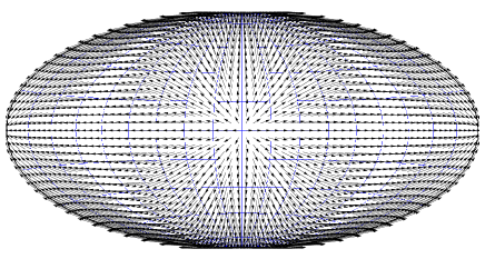
(a) $S_{1,1}$

(b) $S_{2,1}$

(c) $S_{5,3}$

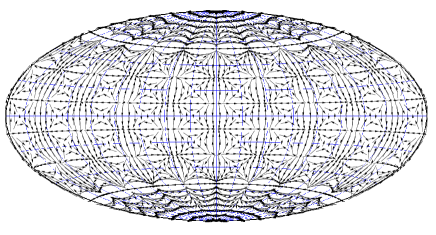
(d) $S_{10,5}$

Figure 2: Examples of spheroidal harmonics vector fields: $S_{1,1}$, $S_{2,1}$, $S_{5,3}$, $S_{10,5}$, where one sees the change in the angular resolution with higher degrees. The $S_{1,1}$ is a glide flow in the direction of the $y$-axis.

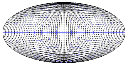
(a) $T_{1,1}$

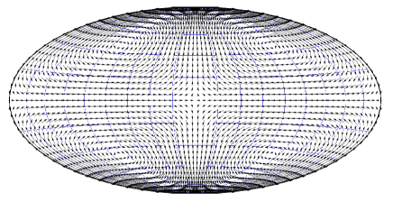
(b) $T_{2,1}$

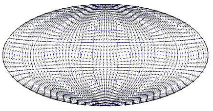
(c) $T_{5,3}$

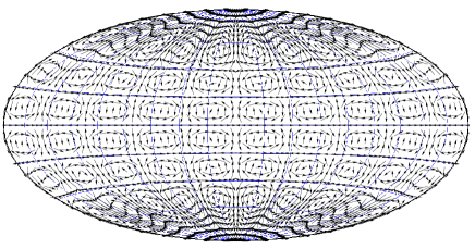
(d) $T_{10,5}$

Figure 3: Examples of toroidal harmonics vector fields: $T_{1,1}$, $T_{2,1}$, $T_{5,3}$, $T_{10,5}$. One sees the change in the angular resolution with higher degrees. The $T_{1,1}$ is a simple rotation about the $y$-axis.

3 Transformation under rotation

3.1 Overview

A very important mathematical and practical feature of the expansion of a vector field on the basis of the VSHs is how they transform under a rotation of the reference axes. In short, when a vector field is given in a frame ${\cal S}$ and decomposed over the VSHs in this frame, one gets the set of components $t_{lm},s_{lm}$ in this frame. Rotating the reference frame ${\cal S}$ (e.g. transforming from equatorial coordinates to galactic coordinates) to the frame $\overline{\cal S}$, one gets the transformed vector field that can be fitted again on a set of VSHs defined in the frame $\overline{\cal S}$. This results in a new set of components $\overline{t}_{lm}$ and $\overline{s}_{lm}$, representing the vector field in this second frame. Significant additional work may be required to carry out the whole transformation of the initial field and perform the fit anew in the rotated frame. Fortunately due to the narrow relationship between VSHs and group representation, there is in fact a dramatic shortcut to this heavy procedure that adds considerably to the interest of using the VSH expansions in astronomy. This is illustrated in the self-explanatory accompanying commutative diagram, showing that to a space rotation (in the usual three-dimensional space) $R$ corresponds to an operator $\mathcal{R}$ acting in the space of the VSHs and allows transforming $t_{lm}$ and $s_{lm}$ given in the initial frame into an equivalent set in the rotated frame:

$$\begin{CD}{\cal S}@>{R}>{}>\overline{\cal S}\\ @V{VSH}V{}V@V{}V{VSH}V\\ \{t_{lm},s_{lm}\}@>{\mathcal{R}}>{}>\{\overline{t}_{lm},\overline{s}_{lm}\}\end{CD}$$

The amount of computation is negligible since this is a linear transformation between the coefficients of a given degree $l$. Overall, the set of $t_{lm}$ and $s_{lm}$ is transformed into itself without mixing coefficients of different degrees.

This operator $\mathcal{R}$ has been introduced by E. Wigner in 1927 as the D-matrices. A convenient reference regarding its definition and properties is the book of Varshalovich, Moskalev & Khersonski (1988). Section 7.3 of that book is specifically devoted to this topic. The Wigner matrices have been used for decades in quantum mechanics, but probably they are not so well known in fundamental astronomy. We confine ourselves here to a quick introduction of the main formulas and conventions used in this paper. All the mathematical formulas have been implemented in computer programs (independently in FORTRAN and Mathematica), which can be requested from the authors.

For practical astronomical applications, there is an unexpected benefit in this transformation under space rotation, which is not shared by the separate analysis on spherical harmonics of the components like $\Delta\alpha\cos\delta$ and $\Delta\delta$, or their equivalent for the proper motions. In general the two components for a given source obtained from observations do not have the same accuracy and are correlated. In the case of space astrometry missions like Hipparcos or Gaia, the correlations are generally smaller in the ecliptic frame due to the symmetry of the scanning in this frame compared to the correlations in the equatorial frame, where the solution is naturally available. Performing a least squares adjustment to compute $t_{lm}$ and $s_{lm}$ with correlated observations is a complication and standard pieces of software often allow only for diagonal weight matrix. One can easily get round this difficulty by carrying out the fitting in a frame where the correlations can be neglected (assuming such a frame does exist), and then rotate the coefficients with the Wigner matrix into the equatorial frame. This is equivalent to rigorously performing the fit in the equatorial coordinates with correlated observations. On the other hand, by fitting the components with scalar spherical harmonics, it is cumbersome to take the correlations between the components properly into account, and the coefficients in one frame do not transform simply into their equivalent into a rotated frame.

More generally, if we allow for the correlations in the frame where the least squares expansion over the VSHs is carried out, one can still apply the Wigner rotation to the results and obtain the expansion in a second frame. The results would be exactly the same as if a new least squares fit had been performed in this frame by rigorously propagating the non-diagonal covariance matrix of the observations to this second frame to generate the new weight matrix. Using the Wigner matrix in this context is conceptually much simpler and in keeping with the underlying group properties of the VSHs, even though there might be no definite advantage for numerical efficiency (but no disadvantage as well).

3.2 Mathematical details

Consider two rectangular Cartesian coordinate systems ${\cal S}$ and $\overline{\cal S}$ of the same handedness. Two coordinate systems are related by a rotation parametrised by three Euler angles $a$, $b$, and $c$. For a given vector with components $x$ in ${\cal S}$, the components $\overline{\mbox{\boldmath$x$}}$ in $\overline{\cal S}$ read as

$$\overline{\mbox{\boldmath$x$}}={\bf R}_{z}(c)\,{\bf R}_{y}(b)\,{\bf R}_{z}(a)\,\mbox{\boldmath$x$},$$ (31)

where ${\bf R}_{z}$ and ${\bf R}_{y}$ are the usual matrix of (passive) rotation, respectively, about axes $z$ and $y$

$${\bf R}_{z}(\varepsilon) = \pmatrix{\cos\varepsilon&\sin\varepsilon&0\cr-\sin\varepsilon&\cos\varepsilon&0\cr 0&0&1},$$ (32)

$${\bf R}_{y}(\varepsilon) = \pmatrix{\cos\varepsilon&0&-\sin\varepsilon\cr 0&1&0\cr\sin\varepsilon&0&\cos\varepsilon\cr}\,,$$ (33)

where the order of arguments in the rotational matrices in (31) must be exactly followed. The inverse transformation reads

$$\mbox{\boldmath$x$}={\bf R}_{z}(-a)\,{\bf R}_{y}(-b)\,{\bf R}_{z}(-c)\,\overline{\mbox{\boldmath$x$}}\,.$$ (34)

Here the convention $z-y-z$ is used for the sequence of rotations instead of the usual $z-x-z$ that is more common in dynamics and celestial mechanics. The former choice has the great advantage of giving a real matrix $d^{l}_{mn}(b)$ (see below) for the intermediate rotation, and this convention is universally used in quantum mechanics and group representation. The values of $a$, $b$, and $c$ for transformations between the three usual frames in astronomy are listed in Table. 1. The relation between the $z-y-z$ and $z-x-z$ conventions is given by

$${\bf R}_{z}(c)\,{\bf R}_{y}(b)\,{\bf R}_{z}(a)={\bf R}_{z}\left(c-\pi/2\right)\,{\bf R}_{x}(b)\,{\bf R}_{z}\left(a+\pi/2\right),$$ (35)

where ${\bf R}_{x}$ are the usual matrix of rotation about axis $x$:

$${\bf R}_{x}(\varepsilon) = \pmatrix{1&0&0\cr 0&\cos\varepsilon&\sin\varepsilon\cr 0&-\sin\varepsilon&\cos\varepsilon\cr}\,.$$ (36)

Then the transformations between the scalar and vector spherical functions defined in ${\cal S}$ and $\overline{\cal S}$ are similar to each other and read as

$$\overline{Y}_{lm}(\overline{\alpha},\overline{\delta}) = \sum_{m^{\prime}=-l}^{l}D^{l}_{m^{\prime}m}(a,b,c)\,Y_{lm^{\prime}}(\alpha,\delta)\,,$$ (37)

$$\overline{\mbox{\boldmath$T$}}_{lm}(\overline{\alpha},\overline{\delta}) = \sum_{m^{\prime}=-l}^{l}D^{l}_{m^{\prime}m}(a,b,c)\,\mbox{\boldmath$T$}_{lm^{\prime}}(\alpha,\delta)\,,$$ (38)

$$\overline{\mbox{\boldmath$S$}}_{lm}(\overline{\alpha},\overline{\delta}) = \sum_{m^{\prime}=-l}^{l}D^{l}_{m^{\prime}m}(a,b,c)\,\mbox{\boldmath$S$}_{lm^{\prime}}(\alpha,\delta)\,,$$ (39)

where $\overline{\alpha}$ and $\overline{\delta}$ are angles defined as right ascension and declination (generally speaking, the longitude and latitude of the spherical coordinates) from the components $\overline{\mbox{\boldmath$x$}}$, while $\alpha$ and $\delta$ are those derived from the components $x$. In both cases Eq. (4) is used. Here $D^{l}_{mn}(a,b,c)$, $|m|\leq l$, $|n|\leq l$ are the Wigner $D$-matrices (generalised spherical functions) defined as

$$D^{l}_{mn}(a,b,c) = e^{-\buildrel\circ\over{\i}\left(m\,a+n\,c\right)}\,d^{l}_{mn}(b),$$ (40)

$$d^{l}_{mn}(b) = (-1)^{m-n}\sqrt{(l+m)!(l-m)!(l+n)!(l-n)!}\,$$ (41)

$$\times\sum_{k=k_{\rm min}}^{k_{\rm max}}(-1)^{k}{{\left(\cos{b\over 2}\right)}^{2l-2k-m+n}{\left(\sin{b\over 2}\right)}^{2k+m-n}\over k!(l-m-k)!(l+n-k)!(m-n+k)!}\,,$$

$$k_{\rm min}=\max(0,n-m),\quad k_{\rm max}=\min(l-m,l+n)\,.$$

Many efficient ways to evaluate $D^{l}_{mn}(a,b,c)$ and $d^{l}_{mn}(b)$ can be found in relevant textbooks. For example, Section 4.21 of Varshalovich, Moskalev & Khersonski (1988) gives the expression of $d^{l}_{mn}(b)$ in the form of a simple Fourier polynomial

$$d^{l}_{mn}(b)=\left(\buildrel\circ\over{\i}\right)^{m-n}\sum_{k=-l}^{l}d^{l}_{km}\left({\pi\over 2}\right)\,d^{l}_{kn}\left({\pi\over 2}\right)\,e^{-\buildrel\circ\over{\i}\,k\,b}\,,$$ (42)

where $d^{l}_{mn}\left({\pi\over 2}\right)$ can be precomputed (using the obvious simplification of (41)) as constants and used in further calculations for a given rotational angle $b$. However, even a straight implementation of (40)–(41) does the job without any problem for low to medium degrees.

The inverse transformations of the spherical functions read as

$$Y_{lm}(\alpha,\delta) = \sum_{m^{\prime}=-l}^{l}D^{l\,\ast}_{m\,m^{\prime}}(a,b,c)\,\overline{Y}_{lm^{\prime}}(\overline{\alpha},\overline{\delta})\,,$$ (43)

$$\mbox{\boldmath$T$}_{lm}(\alpha,\delta) = \sum_{m^{\prime}=-l}^{l}D^{l\,\ast}_{m\,m^{\prime}}(a,b,c)\,\overline{\mbox{\boldmath$T$}}_{lm^{\prime}}(\overline{\alpha},\overline{\delta})\,,$$ (44)

$$\mbox{\boldmath$S$}_{lm}(\alpha,\delta) = \sum_{m^{\prime}=-l}^{l}D^{l\,\ast}_{m\,m^{\prime}}(a,b,c)\,\overline{\mbox{\boldmath$S$}}_{lm^{\prime}}(\overline{\alpha},\overline{\delta})\,,$$ (45)

where the superscript ‘$\ast$’ denotes complex conjugation.

Now what matters for our purpose is the transformation of the VSH coefficients $t_{lm}$ and $s_{lm}$ as in (23) under a rotation of the coordinate system, and, more generally, that of coefficients $f_{lm}$ in the case of an expansion of a scalar field in the scalar spherical harmonics as given by (16).

Given the completeness of the scalar and vector basis functions, we have defined the following expansions for scalar field $f$ and vector field $V$ on sphere (cf. (16) and (23)):

$$f = \sum_{l=0}^{\infty}\sum_{m=-l}^{l}f_{lm}\,Y_{lm}=\sum_{l=0}^{\infty}\sum_{m=-l}^{l}\overline{f}_{lm}\,\overline{Y}_{lm}\,,$$ (46)

$$V = \sum_{l=1}^{\infty}\sum_{m=-l}^{l}\left(t_{lm}\,\mbox{\boldmath$T$}_{lm}+s_{lm}\,\mbox{\boldmath$S$}_{lm}\right)=\sum_{l=1}^{\infty}\sum_{m=-l}^{l}\left(\overline{t}_{lm}\,\overline{\mbox{\boldmath$T$}}_{lm}+\overline{s}_{lm}\,\overline{\mbox{\boldmath$S$}}_{lm}\right).$$ (47)

Substituting (37)–(39) or (43)–(45) into (46)–(47) and changing the order of summations, one gets the important transformation rules for the coefficients

$$f_{lm} = \sum_{m^{\prime}=-l}^{l}D^{l}_{m\,m^{\prime}}(a,b,c)\,\overline{f}_{lm^{\prime}}\,,$$ (48)

$$t_{lm} = \sum_{m^{\prime}=-l}^{l}D^{l}_{m\,m^{\prime}}(a,b,c)\,\overline{t}_{lm^{\prime}}\,,$$ (49)

$$s_{lm} = \sum_{m^{\prime}=-l}^{l}D^{l}_{m\,m^{\prime}}(a,b,c)\,\overline{s}_{lm^{\prime}}\,,$$ (50)

and the inverse transformations

$$\overline{f}_{lm} = \sum_{m^{\prime}=-l}^{l}D^{l\,\ast}_{m^{\prime}m}(a,b,c)\,f_{lm^{\prime}}\,,$$ (51)

$$\overline{t}_{lm} = \sum_{m^{\prime}=-l}^{l}D^{l\,\ast}_{m^{\prime}m}(a,b,c)\,t_{lm^{\prime}}\,,$$ (52)

$$\overline{s}_{lm} = \sum_{m^{\prime}=-l}^{l}D^{l\,\ast}_{m^{\prime}m}(a,b,c)\,s_{lm^{\prime}}\,.$$ (53)

Table 1: Euler angles $a$, $b$ and $c$ applicable to the change of astronomical frame. The obliquity has been taken for J2000 and equatorial frame can be seen as the same as ICRF at this level of accuracy.

Transformation	$a$	$b$	$c$
	deg	deg	deg
Equatorial to Ecliptic	270.0	23.4393	90.0
Equatorial to Galactic	192.8595	62.8718	57.0681
Ecliptic to Galactic	180.0232	60.1886	83.6160

Once the expansion has been computed in one frame, it is very easy to compute the expansion in any other frame related by a rotation from the initial frame. Numerical checks have been performed with the analysis of a vector field in two frames, followed by the transformations (direct and inverse) of the coefficients $t_{lm}$ and $s_{lm})$ with (48)–(50) and (51)–(53).

These transformation rules allow us also to prove the invariance of the Euclidean norm of the set of coefficients of a given degree:

$${\cal P}^{Y}_{l} = \sum_{m=-l}^{l}f_{lm}\,f^{\ast}_{lm}=\sum_{m=-l}^{l}\overline{f}_{lm}\,\overline{f}^{\,\ast}_{lm},$$ (54)

$${\cal P}^{t}_{l} = \sum_{m=-l}^{l}t_{lm}\,t^{\ast}_{lm}=\sum_{m=-l}^{l}\overline{t}_{lm}\,\overline{t}^{\,\ast}_{lm},$$ (55)

$${\cal P}^{s}_{l} = \sum_{m=-l}^{l}s_{lm}\,s^{\ast}_{lm}=\sum_{m=-l}^{l}\overline{s}_{lm}\,\overline{s}^{\,\ast}_{lm}.$$ (56)

This can be easily demonstrated by substituting (48)–(50) into corresponding equation and using the well-known relation

$$\sum_{m=-l}^{l}D^{l}_{m\,m^{\prime}}(a,b,c)\,D^{l\,\ast}_{m\,m^{\prime\prime}}(a,b,c)=\delta_{m^{\prime}m^{\prime\prime}}\,,$$ (57)

which is a special case of the general addition theorem for the Wigner $D$-matrices (Varshalovich, Moskalev & Khersonski 1988, Section 4.7). The invariance of ${\cal P}_{l}$ will be used in Section 5.2 to assess the level of significance of the coefficients.

4 Relation of the first-order VSH to global features

The multipole (VSH) representation of a vector field has some similarity with a Fourier or a wavelet decomposition since as the degree $l$ increases, one sees smaller details in the structure of the field. In the case of the comparison between two catalogues, increasing the degree reveals the zonal errors of the catalogue, while the very first degrees, say $l=1$ and $l=2$, show features with the longer “wavelengths”. In particular, the first degree both in the toroidal and spheroidal harmonics is linked to very global features, such as rotation between the two catalogues or a systematic dipole displacement, like a flow from a source to a sink located at the two poles of an axis. It must be stressed that these global features are found in a blind way, without searching for them. They come out naturally in the decomposition as the features having the least angular resolution, and they are interpreted as a rotation or a dipole glide a posteriori.

4.1 Rotation

Consider a infinitesimal rotation on a sphere given by an the rotation vector $R$ whose components in a particular frame are $(R_{1},R_{2},R_{3})$. This rotation generates the vector field

$$\mbox{\boldmath$V$}^{R}=\mbox{\boldmath$R$}\times\mbox{\boldmath$u$}\,,$$ (58)

where $u$ is the unit radial vector given by (4). Equation (58) can be projected on the local tangent plane and leads to

$$V_{\alpha}^{R} = \mbox{\boldmath$V$}^{R}\cdot\mbox{\boldmath$e$}_{\alpha}=-R_{1}\sin\delta\,\cos\alpha-R_{2}\sin\delta\,\sin\alpha+R_{3}\cos\delta\,,$$ (59)

$$V_{\delta}^{R} = \mbox{\boldmath$V$}^{R}\cdot\mbox{\boldmath$e$}_{\delta}=R_{1}\sin\alpha-R_{2}\cos\alpha\,.$$ (60)

From the explicit expressions of the toroidal harmonics given in Table 6, one sees that any infinitesimal rotation field has non-zero projection only on the $\mbox{\boldmath$T$}_{1m}$ harmonics, and is orthogonal to any other set of toroidal or spheroidal harmonics. Therefore (58) can be written as a linear combination of the $\mbox{\boldmath$T$}_{1m}$. One has explicitly the equivalence

$$\mbox{\boldmath$V$}^{R}=t^{R}_{10}\mbox{\boldmath$T$}_{10}+t^{R}_{11}\mbox{\boldmath$T$}_{11}+t^{R}_{1,-1}\mbox{\boldmath$T$}_{1,-1}$$ (61)

where

$$t_{10}^{R} = \sqrt{\frac{8\pi}{3}}\ R_{3}\,,$$ (62)

$$t_{11}^{R}=-t^{R\,\ast}_{1,-1} = \sqrt{\frac{4\pi}{3}}\ (-R_{1}+\buildrel\circ\over{\i}\,R_{2})\,,$$ (63)

allowing the three parameters $R$ of the rotation to be extracted from the harmonic expansion of degree $l=1$. A change of reference frame will lead to the same rotation vector expressed in the new reference frame. Given the importance of a rotation between two catalogues or in the error distribution of a full sky astrometric catalogue, having the rotational vector field as one of the base functions is a very appealing feature of the VSH. This contrasts with the analysis of each components of the vector on scalar spherical harmonics, in which a plain rotation projects on harmonics of any degree as shown in Vityazev (1997, 2010) or in Appendix C. However, the analysis of each component as scalar fields retains its interest if one has good reasons to assume that the field has been generated by a process in which the two spherical coordinates have been handled more or less separately. In this case there is even no reason to change the frame for another one since the two components may have very different statistical properties.

4.2 Glide

The rotation field is the most common fully global signature on a spherical vector field, and often it even seems to be the only one deserving the qualification of global. However, if we consider a rotational field $\mbox{\boldmath$G$}\times\mbox{\boldmath$u$}$, one may draw at each point on the sphere a vector perpendicular to the rotation field and lying in the tangent plane to the sphere. In this way we generate another field $\mbox{\boldmath$V$}^{G}$ with axial symmetry, fully orthogonal to the rotation field $\mbox{\boldmath$G$}\times\mbox{\boldmath$u$}$. This new field has no projection on the $\mbox{\boldmath$T$}_{1m}$ harmonics and, in fact, on no other $\mbox{\boldmath$T$}_{lm}$. Its components are given by

$$V_{\alpha}^{G} = -G_{1}\sin\alpha+G_{2}\cos\alpha\,,$$ (64)

$$V_{\delta}^{G} = -G_{1}\sin\delta\,\cos\alpha-G_{2}\sin\delta\,\sin\alpha+G_{3}\cos\delta\,,$$ (65)

where the vector $\mbox{\boldmath$G$}=(G_{1},G_{2},G_{3})$ determines the orientation and the magnitude of the field, as $R$ did for the rotational field. Going to Table 6 it is easy to see that it is equivalent to the $\mbox{\boldmath$S$}_{1m}$ field with the decomposition

$$\mbox{\boldmath$V$}^{G}=s^{G}_{10}\mbox{\boldmath$S$}_{10}+s^{G}_{11}\mbox{\boldmath$S$}_{11}+s^{G}_{1,-1}\mbox{\boldmath$S$}_{1,-1}$$ (66)

where

$$s_{10}^{G} = \sqrt{\frac{8\pi}{3}}\,G_{3}\,,$$ (67)

$$s_{11}^{G} = \sqrt{\frac{4\pi}{3}}\,(-G_{1}+\buildrel\circ\over{\i}\,G_{2})\,,$$ (68)

showing its close relationship with a rotation field. A corresponding picture can be seen in Fig. 2 for an axis along the $y$-axis.

The same can be stated somewhat differently: we have introduced the glide vector field $\mbox{\boldmath$V$}^{G}$, which is orthogonal to both radial vector $u$ and the rotation field $\mbox{\boldmath$G$}\times\mbox{\boldmath$u$}$, or equivalently one has

$$\mbox{\boldmath$V$}^{G}=\mbox{\boldmath$u$}\times(\mbox{\boldmath$G$}\times\mbox{\boldmath$u$})=\mbox{\boldmath$G$}-(\mbox{\boldmath$G$}\cdot\mbox{\boldmath$u$})\,\mbox{\boldmath$u$}\,,$$ (69)

which shows clearly that the associated vector field is just the projection of $G$ on the surface of the unit sphere (we have above $G$ minus its radial component), that is to say the projection of an axial, or dipole, field on the sphere.

As a pattern, a glide field is as global a feature as a rotation, and can be seen as a regular flow between a source and a sink diametrically opposed. From the astronomical point of view this is a field associated to a motion of the observer toward an apex, with all the stars showing a kinematical stream in the opposite direction. For extragalactic sources like quasars, this also characterises the effect induced on QSO systematic proper motions resulting from the acceleration of the observers with respect to the frame where the QSOs are at rest on average (Fanselow 1983; Sovers et al. 1998; Kovalevsky 2003; Kopeikin & Makarov 2006; Titov, Lambert & Gontier 2011). The main source of this acceleration is thought to be the centripetal acceleration from the galactic rotation. Its unambiguous determination should be achieved with Gaia. It is important to recognise that in the general analysis of catalogues or spherical vector fields, rotation is not more fundamental a feature than glide, and both must be searched for simultaneously. Otherwise, for most of the distributions of the data on the sphere, when the discrete orthogonality conditions between the VSHs are not fully satisfied, there will be a projection of the element not included in the model in the subspace generated by the other one. Thus, fitting only the rotation, the rotation vector will be biased if there is a glide not accounted for in the data model. And reciprocally for the glide without rotation properly fitted.

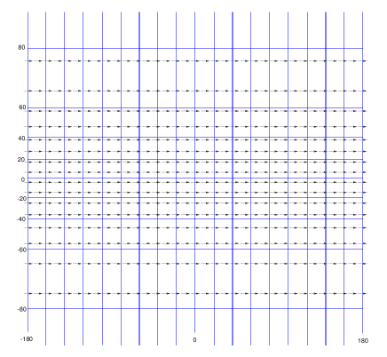
(a) Rotation

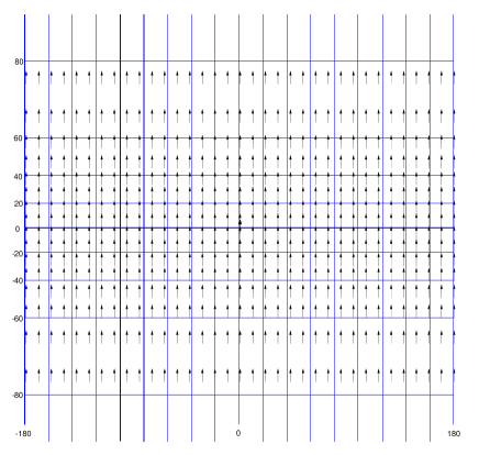
(b) Glide

Figure 4: Rotation and glide with the $z$-axis shown here with a Mercator projection to emphasise the close relationship between the two vector fields. The constant displacement in longitude from the rotation has its counterpart with a constant glide displacement in the reduced latitude (Mercator latitude).

4.3 Duality of the rotation and glide effects

Finally the duality between the infinitesimal rotation and glide can be made striking if the fields are plotted in the Mercator projection, as illustrated in Fig. 4. Both effects are along the $z$-axis and have the same magnitude for $R$ and $G$. Thus they are rotation and glide with the same axis. The effect of a small rotation is seen as a uniform translation in longitude, identical to all latitudes, as expected for a cylindrical projection. For the glide, the translation is uniform in the reduced latitude given by the Mercator transformation

$$\delta_{\mathrm{M}}=\ln\left(\tan\left(\frac{\delta}{2}+\frac{\pi}{4}\right)\right)$$ (70)

and does not depend on the longitude.

There is a clear similarity between the two fields (both represent a mapping of the sphere onto itself with two fixed points: the poles), but also an important difference seen with the Mercator projection: for the rotations, the mapping of a flow line (the continuous line tangent to the vectors of the field) is bound between the two extreme boundaries $-\pi$ and $+\pi$, which must be identified as the same line on the sphere. The rotation axis is the natural source of a cylindrical symmetry shown by the Mercator projection (or any other cylindrical projection). For the glide, it goes very differently since the two end points of a flow line are sent to infinity, in both directions, and can only be identified in the projective space, a much more complex manifold than the Euclidean cylinder. Could this important topological difference be the underlying reason why only the rotation is usually considered as the only obvious global structure? We do not have the answer and leave this issue open for the moment. As long as infinitesimal transformations are concerned, which is exactly what matters for the analysis of astrometric catalogues, the two effects are in fact very similar and must be taken into account together as a whole.

5 Practical implementation

In principle, once the difference between two catalogues has been formed or when a vector field on a sphere (e.g. a set of proper motions) is available, it is normally trivial to project the underlined vector field on the VSH, by computing the integrals (24) with an appropriate numerical methods. This will work as long as the distribution of the sources on the unit sphere preserves the orthogonality conditions between the different base functions. What is precisely meant is the following: using the same numerical method to evaluate the Fourier integrals, one should check that Eqs. (18), (19) and (20) hold with a level of accuracy compatible with the noise up to some degree $l_{\rm max}$. Unless one has many sources almost evenly distributed, this condition is rarely fulfilled. However, the fact that the coefficients can be expressed by integrals, that is to say by direct projection on the base functions, is a simple consequence of the application of a least squares criterion leading to a diagonal normal matrix when the orthogonality condition holds. Starting one step back to the underlying least squares principle we can directly fit the coefficients to the observed components of the field with the model (30), by applying a weighting scheme based on the noise in the data. In case the orthogonality conditions hold, the solution will be equivalent to the evaluation of the integrals. When this assumption is not true, meaning with the discrete sampling and/or uneven weight distribution at the source coordinates, the harmonics are not numerically orthogonal, but the least squares fitting provides an unbiased estimate of the coefficients $t_{lm}$ and $s_{lm}$, together with their covariance matrix.

5.1 Least squares solution

The fitting model is given by (30) up to the degree $l=l_{\rm max}$. It is fitted to a set of $N$ data points sampled at ($\alpha_{k}$, $\delta_{k}$), $k=1,2,\cdots,N$, where at each point the two components of the vector field $\Delta$ (e.g., difference between two catalogues, or proper motion components) are given as

$$\mbox{\boldmath$\Delta$}(\alpha_{k},\delta_{k})=\Delta^{\alpha}_{k}\,\mbox{\boldmath$e$}_{\alpha}+\Delta^{\delta}_{k}\,\mbox{\boldmath$e$}_{\delta},\ k=1,2,\cdots,N\,,$$ (71)

together with the estimates of their associated random noise $\sigma_{\Delta^{\alpha}_{k}}$ and $\sigma_{\Delta^{\delta}_{k}}$. For the sake of simplicity we assume here that the covariance matrix between the observations is diagonal, meaning the observations are realisations of independent random variables. The observations are fitted to the model (30) with the least squares criterion

$$\min_{t_{lm},s_{lm}}\sum_{k=1}^{N}\left(\frac{\left(\Delta^{\alpha}_{k}-V_{\alpha}(\alpha_{k},\delta_{k})\right)^{2}}{\sigma_{\Delta^{\alpha}_{k}}^{2}}+\frac{\left(\Delta^{\delta}_{k}-V_{\delta}(\alpha_{k},\delta_{k})\right)^{2}}{\sigma_{\Delta^{\delta}_{k}}^{2}}\right)\,.$$ (72)

From (30) and (22) we see that with $N$ observations one has $2N$ conditional equations to determine the $2l_{\rm max}(l_{\rm max}+2)$ coefficients $(t_{l0},\,t^{\Re}_{lm},\,t^{\Im}_{lm},\,s_{l0},\,s^{\Re}_{lm},\,s^{\Im}_{lm})$, $m=1,2,\ldots,l$, $l=1,2,\ldots,l_{\rm max}$. The size of the design matrix is $2N\,\times\,2l_{\rm max}(l_{\rm max}+2)$, which can be very large in analysis of astrometric surveys, with $N$ above $10^{5}-10^{6}$ and a sensitivity on a small enough angular scale to represent the regional errors leading to explore up to $l_{\rm max}\sim 15-20$. The data storage could become a problem if one wishes to store and access the full design matrix. One solution to get round this problem is to build up the normal matrix on the fly, taking its symmetry into account. For a large data set ($N\gg l_{\rm max}^{2}$), this bookkeeping part will be the most demanding in terms of computation time. For fixed $N$ the computational time for this part of calculations grows like $l_{\rm max}^{4}$. In general the problem is rather well conditioned, with small off-diagonal terms, and is not prone to generate numerical problems to get the least squares solution.

5.2 Significance level

The least squares solution ends up with an estimate for each of the coefficients included in the model. The model must go to a certain maximum value of $l_{\rm max}$ by including all the component harmonics of order $m$, for each $l\leq l_{\rm max}$. The total number of unknowns is then $2l_{\rm max}(l_{\rm max}+2)$ and grows quadratically with $l_{\rm max}$. Within a degree $l$, one can decide on the significance of each coefficient of order $m$, from its amplitude compared to the standard deviation. However, these individual amplitudes are not invariant by a change of reference frame, like the components of a vector in ordinary space, and the significance of a particular component is not preserved through a rotation of the frame. On the other hand, the whole set of $t_{lm}$ or $s_{lm}$ for a given $l$ behaves like a vector under rotation, and the significance (or lack of) of the vector itself, that is to say its modulus, is intrinsic and remains true or false in any other rotated frame. Therefore it is more interesting and more useful in practice to investigate the significance level for each degree $l$ rather than that of the individual coefficients. The reason behind this statement is deeply rooted in the invariance property of the $Y_{lm}$ under a rotation in the three-dimensional Euclidean space and the fact that the set of spherical harmonics $Y_{lm}$ of degree $l$ is the basis of an irreducible representation of the rotation group of the usual three-dimensional space. Therefore, this set is globally invariant under a rotation, meaning there is linear transformation linking the $Y_{lm}$ in one frame to their equivalent of same degree $l$ in the other frame (see Section 3).

Therefore, one should consider the $2l+1$ elements of the set $Y_{lm}$, for $m=-l,\dots l$ like the components of a vector that are transformed into each other under a rotation, keeping the Euclidean norm unchanged in the process. Given the linearity of the derivative operator, this property extends naturally to the $\mbox{\boldmath$T$}_{lm}$ and $\mbox{\boldmath$S$}_{lm}$. For the same reason, the coefficients $t_{lm}$ and $s_{lm}$ in the expansion of a vector field must be considered together within a degree $l$ and not examined separately, unless one has good reasons to interpret physically one or several coefficients in a particular frame: the Oort coefficients in the Galactic frame are one of the possible examples, as shown in Vityazev (2010). More generally a wide range of parameters in Galactic kinematics have very natural representations on vector harmonics, such as the solar motion towards the apex or a more general description of the differential rotation than the simple Oort’s modelling (see for example Mignard (2000)).

Therefore it is natural to look at the power of the vector field and at how this power is spread over the different degrees $l$. Let $\mathcal{P}$ be the power of a real vector field $\mbox{\boldmath$V$}(\alpha,\delta)$ on a sphere defined by the surface integral,

$$\mathcal{P}(\mbox{\boldmath$V$})=\int_{\Omega}\,|\mbox{\boldmath$V$}|^{2}\,d\Omega\,,$$ (73)

or its discrete form used hereafter with numerical data,

$$\mathcal{P}(\mbox{\boldmath$V$})\simeq\frac{4\pi}{n}\sum_{i=1}^{n}|\mbox{\boldmath$V$}_{i}|^{2}\,,$$ (74)

where $n$ is the number of samples on the sphere.

When projected on the VSH one finds easily with (18), (19), and (23) that

$$\mathcal{P}(\mbox{\boldmath$V$}) = \sum_{l=1}^{l_{\rm max}}\left(\mathcal{P}^{t}_{l}+\mathcal{P}^{s}_{l}\right)\,,$$

$$\mathcal{P}^{t}_{l} = \sum_{m=-l}^{l}t_{lm}\,t^{\ast}_{lm}\,,$$

$$\mathcal{P}^{s}_{l} = \sum_{m=-l}^{l}s_{lm}\,s^{\ast}_{lm}\,.$$ (75)

For a real vector field having the symmetries (26)–(27) one gets

$$\mathcal{P}^{t}_{l} = t_{l0}^{2}+2\sum_{m=1}^{l}|t_{lm}|^{2}=t_{l0}^{2}+2\sum_{m=1}^{l}\left((t_{lm}^{\Re})^{2}+(t_{lm}^{\Im})^{2}\right)\,,$$

$$\mathcal{P}^{s}_{l} = s_{l0}^{2}+2\sum_{m=1}^{l}|s_{lm}|^{2}=s_{l0}^{2}+2\sum_{m=1}^{l}\ \left(\,(s_{lm}^{\Re})^{2}+(s_{lm}^{\Im})^{2}\right)\,.$$ (76)

The quantities $\mathcal{P}^{t}_{l}$ and $\mathcal{P}^{s}_{l}$ are the powers of toroidal and spheroidal components of the degree $l$ of the field. Both quantities are scalars invariant under rotation of the coordinate system (see Section 3). Thus $\mathcal{P}^{t}_{l}$ and $\mathcal{P}^{s}_{l}$ represent an intrinsic property of the field, similar to the magnitude of a vector in an ordinary Euclidean vector space.

We can now take up the important issue of the significance level of the subset of the coefficients $s_{lm}$ and $t_{lm}$ for each degree $l$. In harmonic or spectral analysis, this is always a difficult subject, because it needs to scale the power against some typical value that would be produced by a pure noisy signal. In general one can construct a well-defined test, with secure theoretical foundations, but with assumptions about the time or space sampling, which are rarely found in the real world. Therefore the theory provides a good guideline, but not necessarily a fully safe solution applicable in all situations. The key issue here is to construct a criterion that is well understood from the statistical view point and robust enough to be usable for mild departure from the underlying assumptions, like regular time sampling in time series. We offer below three possibilities for testing whether the power $\mathcal{P}^{t}_{l}$ and $\mathcal{P}^{s}_{l}$ is significant and therefore that there is a true signature of the VSH of degree $l$ in the vector field. In the following we drop superscripts ‘$s$’ and ‘$t$’ and write simply $\mathcal{P}_{l}$. Relevant formulas below are valid separately for $\mathcal{P}^{t}_{l}$ and $\mathcal{P}^{s}_{l}$ or for $\mathcal{P}^{t}_{l}+\mathcal{P}^{s}_{l}$. The involved coefficients will be denoted as $r_{lm}$ to represent either $t_{lm}$ or $s_{lm}$ or both.

Start from the null hypothesis $H_{0}$ that the signal is just made of noise, producing some values of $\mathcal{P}_{l}$ in the analysis. One needs to build a test to tell us that above a certain threshold, the value of $\mathcal{P}_{l}$ is significant and would only be produced by pure noise with a probability $p\ll 1$. To build the test properly, the probability density function (PDF) of $\mathcal{P}_{l}$ is required. It can be obtained with the additional assumptions that the sources are rather evenly distributed on the sphere. The least squares fitting also gives us the variance-covariance matrix of the unknowns $s_{lm}$ and $t_{lm}$. Given the orthogonality properties of the VSH, the normal matrix is almost diagonal if the distribution of sources over the sky and the associated errors of the quantity representing the vector field are homogeneous. In this case the covariance matrix is also almost diagonal.

Consider the coefficients $r_{l0}$, $r_{lm}^{\Re}$, and $r_{lm}^{\Im}$ in (30) with a fixed degree $l$. Each diagonal term of the relevant part of the normal matrix (unweighted here) takes the form

$$\phantom{4}\sum R_{l0}^{2} \mathrm{\hskip 28.45274ptfor\hskip 28.45274pt} r_{l0}\,,$$ (77)

$$4\sum(R_{lm}^{\Re})^{2} \mathrm{\hskip 28.45274ptfor\hskip 28.45274pt} r_{lm}^{\Re}\,,$$ (78)

$$4\sum(R_{lm}^{\Im})^{2} \mathrm{\hskip 28.45274ptfor\hskip 28.45274pt} r_{lm}^{\Im}\,,$$ (79)

where the sum extends over all the sources on the sphere. Here $R_{lm}$ stands for either $T_{lm}$ or $S_{lm}$. The first term with $m=0$ does not depend on the right ascension $\alpha$, while the others have a part in $\cos^{2}\!m\alpha$ and $\sin^{2}\!m\alpha$, whose average is $1/2$ for $\alpha$ ranging from $0$ to $2\pi$ and a relatively regular distribution in $\alpha$. Given the normalisation of the VSHs, we now see that the diagonal terms with $m\neq 0$ are just two times the term with $m=0$. The covariance matrix being the inverse of the normal matrix, one eventually has the variances of the unknowns as

$$\mathrm{var}(r_{l0}) = \sigma^{2}_{l0}\,,$$ (80)

$$\mathrm{var}(r_{lm}^{\Re}) = \sigma^{2}_{l0}/2\,,$$ (81)

$$\mathrm{var}(r_{lm}^{\Im}) = \sigma^{2}_{l0}/2\,,$$ (82)

where $\sigma^{2}_{l0}$ is the variance of $r_{l0}$. Then dividing $\mathcal{P}_{l}$ in (5.2) by $\sigma^{2}_{l0}$ leads to the normalised power:

$$W_{l}=\frac{\mathcal{P}_{l}}{\sigma^{2}_{l0}}=\frac{r_{l0}^{2}}{\sigma^{2}_{l0}}+\sum_{m=1}^{l}\,\left(\frac{(r_{lm}^{\Re})^{2}}{\sigma^{2}_{l0}/2}+\frac{(r_{lm}^{\Im})^{2}}{\sigma^{2}_{l0}/2}\right).$$ (83)

With (81)–(82) and the assumption that the signal is pure white Gaussian noise, this is the sum of $2l+1$ squares of standard normal random variables with zero mean and unit variance. It is well known that $W_{l}$ follows a $\chi^{2}$ distribution with $n=2l+1$ degrees of freedom. With this normalisation, $W_{l}$ is strictly proportional to the power $\mathcal{P}_{l}$.

Under the $H_{0}$ hypothesis that the signal is just white noise, one can build a one-sided test to decide whether a harmonic of degree $l$ is significant with the probability level $\gamma$:

$$P(W_{l}>w)=1-\int_{0}^{w}\chi^{2}_{2l+1}(x)dx={\Gamma(l+1/2,w/2)\over\Gamma(l+1/2)}<\gamma\,,$$ (84)

where $\Gamma(a,x)$ and $\Gamma(a)$ are the incomplete and complete gamma functions, respectively. This quantity can be easily computed. In some cases it may be easier to use the transformation of Wilson & Hilferty (1931),

$$Z=\sqrt{\frac{9n}{2}}\left[\,\left(\frac{W_{l}}{n}\right)^{1/3}-\left(1-\frac{2}{9n}\right)\,\right]\,,$$ (85)

where $n$ is the number of degrees of freedom. It is well known that $Z$ approximately follows, even for small $n$, a standard normal distribution of zero mean and unit variance. A test risk of $\gamma=0.01$ is achieved if $Z>2.33$ or at the level of $\gamma=0.025$ is $Z>1.96$. Experiments on simulated data have shown that the key elements in the above derivation, namely that $\sigma_{l0}\simeq\sqrt{2}\,\sigma_{lm},m>0$ is practically achieved when sources are rather regularly distributed in longitudes, even with irregularities in latitudes. The reason is basically that this factor $\sqrt{2}$ follows from the average of $\cos^{2}m\alpha$ and $\sin^{2}m\alpha$, while the latitude effects are shared in a similar way in all the $r_{lm}$.

Alternatively, instead of scaling the power by only $\sigma^{2}_{l0}$ and taking advantage of the asymptotic properties (80)–(82), it would have been more natural to define a reduced power with

$$\widetilde{W_{l}}={\left(\frac{r_{l0}}{\sigma_{l0}}\right)}^{2}+\sum_{m=1}^{l}\ \left({\left(\frac{r_{lm}^{\Re}}{\sigma_{lm}^{\Re}}\right)}^{2}+{\left(\frac{r_{lm}^{\Im}}{\sigma_{lm}^{\Im}}\right)}^{2}\right)\,,$$ (86)

which is not strictly proportional to the power. But what matters in practice is whether one can construct an indicator, related to the power, with well defined statistical properties, so one may relax the constraint of having exactly the power, provided that a reliable test of significance can be built. For least squares solutions with Gaussian noise, and small correlations between the estimates of the unknowns, it is known that each coefficient follows a normal distribution of zero mean whose variances can be estimated with the inverse of the normal matrix. Therefore, $\widetilde{W_{l}}$ is also a sum of squares of standard normal variables and its PDF is that of a $\chi^{2}$ distribution with $2l+1$ degrees of freedom. For regular distributions of the data points, the two reduced powers ${W_{l}}$ and $\widetilde{W_{l}}$ are equivalent. So either test should give the same result. In (86) the multiplying factor two before the sum in (5.2) has been absorbed by $\mathrm{var}(\sqrt{2}Y)=2\,\mathrm{var}(Y)$ (i.e. by $\sigma_{lm}^{\Re}$ and $\sigma_{lm}^{\Im}$ being approximately a factor $\sqrt{2}$ smaller than $\sigma_{l0}$).

Finally, we can also go back to the first test in (83), which is the power scaled by the variance of the component $s_{l0}$. Since the variance ${\sigma^{2}_{l0}}$ is in practice an estimate of a random variable based on the data, it may happen that the value produced by the least squares is unusually small, which will make ${W_{l}}$ too large and trigger a false detection. Therefore, while this test has a good statistical foundation for regular distribution of sources, it is not very robust to departure from this assumption. We suggest improving this robustness, a very desirable feature in the real data processing, by replacing the scaling factor $\sigma^{2}_{l0}$ by the average of the set $\left(\,\sigma^{2}_{l0},2(\sigma_{lm}^{\Re})^{2},2(\sigma_{lm}^{\Im})^{2}\,\right)$, $m=1,\ldots,l$ whose mathematical expectation is the true value of $\sigma^{2}_{l0}$, but it has a smaller scatter than $\sigma^{2}_{l0}$. Let $\bar{\sigma}^{2}_{l0}$ be this average, we have then instead of (83) a new expression for the reduced power

$$\bar{W}_{l}=W_{l}\,\frac{\sigma^{2}_{l0}}{\bar{\sigma}^{2}_{l0}}=\frac{{\cal P}_{l}}{\bar{\sigma}^{2}_{l0}}\,,$$ (87)

which is directly proportional to the power and follows a $\chi^{2}$ distribution with $2l+1$ degrees of freedom.

From a theoretical standpoint, the three indicators are equivalent for a large number of data points evenly distributed on a sphere. In practical situations, with some irregularities in the angular distribution and/or a limited number of sources, the significance testing with $\bar{W}_{l}$ should by construction be more robust against random scatter affecting the estimated standard deviations. Preliminary experiments have confirmed this feature, although a wider Monte Carlo simulation is needed to quantify the advantage.

6 Application to FK5 Catalogue

The comparison between the FK5 and Hipparcos was published soon after the release of the Hipparcos catalogue by Mignard & Froeschlé (2000) primarily provides the orientation and the rotation (spin) of the FK5 system with respect to the Hipparcos frame. The differences in position and proper motions are shown in Fig. 5 for the whole set of stars used in the comparison. In the positional plot one clearly sees a general shift toward the south celestial pole and few regional effects of smaller scales.

The global analysis carried out at that time was restricted to fitting these six parameters from the positional and proper motion differences from Hipparcos to enable the transformation of astronomical data from the FK5 frame into the Hipparcos frame or, more or less equivalently, to the ICRF. The remaining residuals were large and considered as zonal errors, not reducible to a simple representation and presented in the form of plots of $\Delta\alpha\cos\delta$ and $\Delta\delta$ as a function of the position of the stars. Large zonal errors were clearly shown by these plots, but no attempt was made to model these residuals.

Using the VSH now, with the software developed during this work, it is possible to draw refined conclusions and to show that the terms of low degree beyond the rotation are truly significant. In particular we can see in Table 3 that the positional glide term from the spheroidal harmonic of degree $l=1$ is larger than the orientation term. Terms of degree $l=2$ are also large, both in position and proper motion, a feature that had not been noticed as clearly with the earlier analysis based on a priori model.

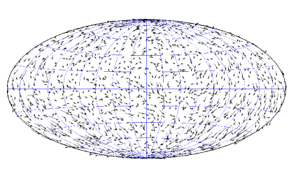
(a) Positions

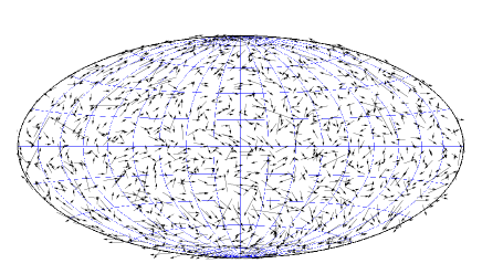
(b) Proper motions

Figure 5: Differences in positions and proper motions between the FK5 catalogue and Hipparcos in 1991.25. The typical arrow sizes in the plots are respectively 100 mas and 2.5 mas/yr.

6.1 Global differences

This concerns the rotation and the glide between the two systems, or equivalently using the VSH terminology, the toroidal and spheroidal harmonics with $l=1$. The results for the rotation shown in Table 2 are fully compatible with the earlier analysis of Mignard & Froeschlé (2000) and confirm a systematic difference between the FK5 inertial frame and the ICRS materialised by Hipparcos. The interpretation of the systematic spin is also discussed in the same paper and seems to be related to the precession constant. These new values also agree with a similar analysis performed by Schwan (2001), provided the epoch is corrected from 1949.4 (mean epoch of the FK5 observations) to 1991.25 (Hipparcos Catalogue reference epoch). A new result is given in Table 3 for the glide, but is only significant in the positions. It describes a systematic difference of about $60\,\cos\delta$  mas in the declination system between the two frames. This is a very large systematic effect given the claimed accuracy of the FK5 below $50$ mas. Nothing similar is seen for the proper motions. Any transformation of a catalogue tied by its construction to the FK5 system and later on aligned to the HCRF (Hipparcos frame aligned to the ICRF) must absolutely take this large systematic difference into account in addition to the rotation. The results just shown correspond to the harmonics $l=1$ from a fit of the position and proper motion difference to $l_{\rm max}=10$. They are slightly different with another choice of the maximum degree, but within the formal error. In both tables the standard deviations quoted are derived from the covariance matrix of the least squares solution scaled by the r.m.s. of the post-fit residuals.

Table 2: Global orientation (in 1991.25) and spin between the FK5 and the Hipparcos catalogue.

Position (mas)			PM(mas/yr)
	J1991.25	$\sigma$			$\sigma$
$\epsilon_{x}$:	-18.1	2.4	$\omega_{x}$:	-0.37	0.09
$\epsilon_{y}$:	-14.6	2.4	$\omega_{y}$:	-0.57	0.09
$\epsilon_{z}$:	-18.5	2.4	$\omega_{z}$:	-0.82	0.09

Table 3: Glide between the FK5 and the Hipparcos catalogue in positions (in 1991.25) and proper motions.

Position (mas)			PM(mas/yr)
	J1991.25	$\sigma$			$\sigma$
$g_{x}$:	-18.3	2.4	$\gamma_{x}$:	-0.04	0.09
$g_{y}$:	-1.3	2.4	$\gamma_{y}$:	-0.18	0.09
$g_{z}$:	-64.0	2.4	$\gamma_{z}$:	-0.37	0.09

6.2 Regional differences

The analysis at higher degree, up to $l=10$, clearly shows significant power in most degrees, indicating a definite structure in the space distribution of the differences. Given the absence of zonal error in the Hipparcos catalogue, at the level seen in this analysis, they must come entirely from the FK5. A detailed analysis of this regions variations was performed by Schwan (2001) by projecting separately each components (difference in right ascension and declination) on a set of scalar orthogonal polynomials, instead of using the vectorial nature of the differences. Given the numerous positional instruments used to produce the FK5, some measuring only the right ascension, others only the declination, others giving both, analysing the components in equatorial coordinates separately makes sense and may reveal structure scattered in many degrees with the VSHs. Here we simply want to illustrate the relevance of the VSH to analyse the difference between two real catalogues. A detailed discussion of the application to the FK5 system is deferred to an independent paper.

6.2.1 Regional differences in position

The amplitudes, defined as the square root of the unweighted power, in each degree for the positional differences between the FK5 and Hipparcos in 1991.25 are given in Table 3, for the toroidal (left part of the table) and spheroidal (right part of the table) harmonics. The level of significance computed with Eq.(87) and the normal approximation of Eq. (85) is shown in the columns labelled $Z$. With $l=1$ one recovers the very large significance of the rotation and the glide. Harmonics $l=2$ are also very large, explaining together with the glide a significant part of the systematic differences between the two catalogues. Then the powers remain statistically very significant up to $l=7$, although with small amplitudes, and then decline. With the values of the $t_{lm}$ and $s_{lm}$ (not given here), one could produce an analytical transformation relating the two systems, in the same spirit as in Schwan (2001). With the last column one sees that the expansion to $l=10$ explains about $58\%$ of the variance seen in the data for the position and $32\%$ for the proper motion.

Table 4: Amplitude (power^1/2) and significance level based on (87) for the positional differences between FK5 and Hipparcos expanded on the VSH.

degree	$\left(\sum_{m}t^{2}_{l\,m}\right)^{1/2}$	Z	$\left(\sum_{m}s^{2}_{l\,m}\right)^{1/2}$	Z	Rem. (power)1/2
	mas		mas		mas
0					474.5
1	85.8	10.18	192.8	19.90	425.0
2	96.6	11.48	139.5	15.94	389.6
3	53.6	6.01	52.8	5.89	382.3
4	65.6	7.44	66.2	7.52	370.8
5	96.8	11.41	62.2	6.72	352.5
6	65.2	6.95	82.2	9.36	336.5
7	68.3	7.18	42.2	3.00	326.7
8	45.0	3.18	57.1	5.22	318.6
9	31.1	0.28	41.4	2.25	314.3
10	34.4	0.63	50.6	3.63	308.3

6.2.2 Regional differences in proper motions

The same analysis has been done for the proper motions. The powers and their significance level expressed with a standard normal variable are listed in Table 4. Again the signal is strong in the harmonics of the first two degrees and up to $l=7$ primarily for the toroidal components.

Table 5: Amplitude (power^1/2) and significance level based on (87) for the proper motion differences between FK5 and Hipparcos expanded on the VSH.

degree	$\left(\sum_{m}t^{2}_{l\,m}\right)^{1/2}$	Z	$\left(\sum_{m}s^{2}_{l\,m}\right)^{1/2}$	Z	Rem. (power)1/2
	mas/yr		mas/yr		mas/yr
0					14.6
1	3.1	9.85	1.2	3.67	14.2
2	2.3	7.40	2.5	8.00	13.8
3	1.1	2.10	1.5	3.88	13.7
4	1.9	5.46	1.9	5.47	13.4
5	2.7	7.97	1.3	2.34	13.1
6	2.0	5.16	1.8	4.33	12.8
7	2.8	8.02	1.3	1.44	12.4
8	1.2	0.52	1.5	2.26	12.3
9	1.3	1.17	1.2	0.28	12.2
10	1.7	2.91	1.2	-0.04	12.0

7 Analysis of the expected Gaia results

Another important application of the VSH technique is an analysis of mathematical properties (e.g. systematic errors) of an astrometric catalogue, as well as extraction of physical information from the catalogue. Here we concentrate on the QSO catalogue as part of the expected Gaia catalogue. Our goal is to investigate (i) the anticipated accuracy of the determination of the rotational state of the reference frame and the acceleration of the solar system with respect to the QSOs, and (ii) the expected estimate of the energy flux of the primordial (ultra-low-frequency) gravity waves. From the mathematical point of view, this amounts to checking the accuracy of determining the VSH coefficients of orders $l=1$ and $l=2$. The toroidal coefficients of order 1 describe the rotational state of the reference frame with respect to the QSOs, while the spheroidal coefficients of order 1 give the acceleration of the solar system with respect to the QSOs, which shows up as a glide (Fanselow 1983; Sovers et al. 1998; Kovalevsky 2003; Kopeikin & Makarov 2006; Titov, Lambert & Gontier 2011). The VSH coefficients of order 2 can be related to the energy flux of the ultra-low-frequency gravity waves (Gwinn et al. 1997).

7.1 Simulated QSO catalogue from Gaia

We simulated the Gaia QSO catalogue with all the details that we know at the time of writing. The total number of QSOs observable by Gaia – 700 000 – was chosen according to the analysis of Mignard (2012). The realistic distribution of the QSOs in the Gaia integrated magnitude $G$ was taken from Slezak & Mignard (2007) (see also Robin et al. 2012). The distribution of the Gaia-observed QSOs over the sky was chosen according to the standard Gaia extinction model (Robin et al. 2012). The model follows the realistic distribution of the dust in the Galaxy, so that the QSO distribution used in this section is not homogeneous on the sky and depends on both angular coordinates with the most pronounced feature being the avoidance area close to the Galactic plane. The proper motions of QSOs are generated from a randomly selected rotation of the reference frame and an acceleration of the solar system’s barycentre with respect to the QSOs with magnitude and direction expected from the circular motion of the solar system with respect to the galactic centre (i.e. the proper motions are generated from the full set of VSH coefficients of order 1). These resulted in our simulated “true” (noise-free) catalogue of QSOs.

The expected accuracies of astrometric parameters (positions, proper motions, and parallaxes) as functions of the $G$ magnitude and the position on the sky are taken from the standard Gaia science performance model (ESA 2011; de Bruijne 2012). Then the QSO simulated solution with Gaia is obtained by adding Gaussian noise with the corresponding standard deviation to each parameter of each source.

One more feature used in our simulations is that we take the correlations between the estimates of the two components of proper motion into account. As a model for the correlations, the empirical distribution is calculated from the corresponding histogram for the Hipparcos catalogue as shown on Fig. 3.2.66 of ESA (1997, vol.1, Section 3.2). We neglect herewith the complicated distribution of the correlation on the sky as shown on Figs. 3.2.60 and 3.2.61 of ESA (1997). The generated random correlation is then used to generate correlated Gaussian noise for the components of the proper motion of each source.

7.2 Main results of the analysis of the simulated QSO catalogue

From the resulting realistic QSO catalogue expected from Gaia, we fitted the VSH coefficients for maximal order $l_{\max}$ ranging from 1 to 15. The correlations between the components of the proper motion for the same star are taken into account in the fit by using block diagonal weight matrix with $2\times 2$ blocks corresponding to each source. Accounting for these correlations in the fit generally modifies the estimates at the level of one tenth of the corresponding standard deviations. We repeated these simulations (including generation of the QSO catalogue) tens of times. For a typical simulation, the resulting biases of the estimates of the rotation of the reference frame and the acceleration of the solar system, as well as the standard errors of those estimates are shown in Fig. 6. The biases are computed as differences between the estimated values and true ones (those put in the simulated ‘noise-free’ catalogue). For the standard errors of the estimates, we took the formal standard deviations from the fit multiplied by the square root of the reduced $\chi^{2}$ of the fit. Comparing of the estimates for different values of $l_{\max}$ as shown in Fig. 6 is a useful indicator of the reliability of the estimate. Our analysis generally confirms the assessments of the anticipated Gaia accuracy for the reference frame and acceleration published previously: both the rotational state of the reference frame and the acceleration of the solar system could be assessed with an accuracy of about 0.2 $\mu$as/yr. However, this accuracy can only be reached under the assumption that (1) Gaia will be successfully calibrated down to that level of accuracy (that is, the errors of astrometric parameters remain Gaussian down to about 0.2 $\mu$as), and (2) real proper motions of the QSOs (transverse motions of the photocentres due to changing QSO structure, etc.) are not too large and do not influence the results. Whether these assumptions are correct will not be known before Gaia flies.

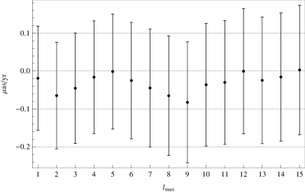
(a) Rotation

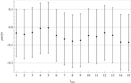
(b) Acceleration (divided by the light velocity)

Figure 6: True errors and formal errors of the estimates of the absolute values of the rotation and acceleration from the fits with $1\leq l_{\max}\leq 15$ for the simulated QSO catalogue matching expected Gaia accuracy.

Finally, we discuss the expected upper estimate of the energy flux of the ultra-low-frequency gravity waves that Gaia could measure. We use the computational recipe described by Gwinn et al. (1997, see Eq. (11) and the discussion in the first paragraph of their Section 4). Our analysis shows that Gaia can be expected to give an estimate at the level of $\Omega_{\rm GW}<0.00008\,h^{-2}$ for the integrated flux with frequencies $\nu<6.4\times 10^{-9}\,{\rm Hz}$. Here, $h=H/(100{\rm km/s/Mpc})$ is the normalised Hubble constant. This is to be compared with the VLBI estimate $\Omega_{\rm GW}<0.11\,h^{-2}$ for $\nu<2\times 10^{-9}\,{\rm Hz}$ of Gwinn et al. (1997). The same approach applied to the VLBI catalogue used by Titov, Lambert & Gontier (2011) gives $\Omega_{\rm GW}<0.009\,h^{-2}$ for $\nu<1.5\times 10^{-9}\,{\rm Hz}$. Therefore, one can expect that Gaia will improve current estimates from VLBI data by two orders of magnitude while covering a larger interval of frequencies. However, this conclusion relies on the ability to see large-scale features of small amplitude in the Gaia proper motion thanks to the improvement of the detection in $1/N_{\mathrm{sources}}^{1/2}$. This can be hindered by correlated noise in the intermediates results or more likely the various sorts of unmodelled systematic errors, not known today, although every effort is made in the instrument design and manufacturing to keep them low and compatible with the above results. These systematic errors can be expected to influence lower degree VSH coefficients to a greater extent than the higher degree ones. Therefore, for analysing the gravity waves, it is advantageous to use not only the quadrupole harmonics as in Gwinn et al. (1997) and Titov, Lambert & Gontier (2011), but also an ensemble of harmonics that includes higher order harmonics (see e.g. Book & Flanagan 2011). Given the number of QSOs in the Gaia catalogue, such a refined approach is feasible and will help establish more reliable limits on the energy flux resulting from primordial gravitational waves.

7.3 Correlations between the VHS coefficients

It is interesting to briefly discuss the correlations between the VSH harmonics resulting from the least squares fits with the simulated catalogue of 700 000 QSOs described above. These correlations were computed form the inverse of the weighted normal matrix from the VHS fit. Depending on the maximal order $l_{\max}$, the root mean square value of the correlations is 0.04, while a few correlations may attain the level of 0.4. Having such a large number of sources one might expect that the correlations should be extremely small. Indeed, for a catalogue of 700 000 sources homogeneously distributed on the sky, the r.m.s. of the correlations between the VSH coefficients is typically 0.0006 and the maximum is at the level of 0.006. We see that the correlations for the realistic QSO catalogue are about 70 times larger. One can find two reasons for the larger correlations: (1) the inhomogeneous distribution of the QSOs on the sky (this can be called the “kinematical inhomogeneity” of the catalogue) and (2) the fact that the accuracies of the QSOs’ proper motions, which are used in the weight matrix, also depend on the position on the sky (this can be called the “dynamical inhomogeneity” of the catalogue). For the QSO catalogue used in this section the dynamical inhomogeneity alone gives correlations with an r.m.s. of 0.01 and the maximum of 0.2, while the kinematical inhomogeneity alone leads to the r.m.s. of 0.03 and the maximum of 0.35. Generally speaking, correlations lead to higher errors in the fitted parameters. We finally note that the dynamical inhomogeneity will be slightly greater for the real Gaia catalogue than we see in our simulation. This is caused by the fact that the standard Gaia science performance model (ESA 2011; de Bruijne 2012) is smoothed in the galactic longitude. However, our calculations show that this additional inhomogeneity does not significantly change the results given above.

8 Conclusion

In this paper we have shown the relevance of the vector spherical harmonics (VSH) to decomposing, more or less blindly, spherical vector fields frequently encountered in astronomical context. This happens very naturally in comparing of stellar positional or proper motion catalogues or the different solutions produced during the data analysis in global astrometry. We have provided the mathematical background and considered several practical issues related to the actual computation of the VSH.

We have in particular:

• shown how to perform the decomposition with a least squares minimisation, enabling processing of irregularly distributed sets of points on the sphere;

• provided a way to test the significance level of any degree in the expansion and then set a criterion for where to stop the expansion;

• stressed the importance of the invariance properties against rotation of the expansion and given the necessary formulas that express the decompositions in the most common astronomical frames;

• provided applications with a reanalysis of the FK5 catalogue compared to Hipparcos, and an example of how this tool should be used during the Gaia data processing to prepare the construction of the inertial frame and derive important physical parameters;

• compiled an extensive set of practical expressions and properties in the Appendices.

Appendix A Explicit formulas for the vector spherical functions with $l\leq 4$

Table 6: Toroidal harmonics $\mbox{\boldmath$T$}_{lm}(\alpha,\delta)$ and spheroidal harmonics $\mbox{\boldmath$S$}_{lm}(\alpha,\delta)$ for $1\leq l\leq 4$.

Harm.	Mult.	Components
	coef.	$\mbox{\boldmath$e$}_{\alpha}$	$\mbox{\boldmath$e$}_{\delta}$
$\mbox{\boldmath$T$}_{10}$	$\frac{1}{2}\sqrt{\frac{3}{2\pi}}$	$\cos\delta$	$0$
$\mbox{\boldmath$T$}_{11}$	$\frac{1}{4}\sqrt{\frac{3}{\pi}}$	$\sin\delta\,(\cos\alpha\,+\buildrel\circ\over{\i}\/\sin\alpha)$	$-\sin\alpha\,+\buildrel\circ\over{\i}\/\cos\alpha$
$\mbox{\boldmath$T$}_{20}$	$\frac{1}{4}\sqrt{\frac{15}{2\pi}}$	$\sin 2\delta$	$0$
$\mbox{\boldmath$T$}_{21}$	$\frac{1}{4}\sqrt{\frac{5}{\pi}}$	$-\cos 2\delta\,(\cos\alpha\,+\buildrel\circ\over{\i}\/\sin\alpha)$	$-\sin\delta\,(\sin\alpha\,-\buildrel\circ\over{\i}\/\cos\alpha)$
$\mbox{\boldmath$T$}_{22}$	$\frac{1}{8}\sqrt{\frac{5}{\pi}}$	$-\sin 2\delta\,(\cos 2\alpha\,+\buildrel\circ\over{\i}\/\sin 2\alpha)$	$2\cos\delta\,(\sin 2\alpha\,-\buildrel\circ\over{\i}\/\cos 2\alpha)$
$\mbox{\boldmath$T$}_{30}$	$\frac{1}{8}\sqrt{\frac{21}{\pi}}$	$\cos\delta\,(5\sin^{2}\delta-1)$	$0$
$\mbox{\boldmath$T$}_{31}$	$\frac{1}{16}\sqrt{\frac{7}{\pi}}$	$\sin\delta\,(15\sin^{2}\!\delta-11)\,(\cos\alpha\,+\buildrel\circ\over{\i}\/\sin\alpha)$	$-(5\sin^{2}\!\delta-1)\,(\sin\alpha\,-\buildrel\circ\over{\i}\/\cos\alpha)$
$\mbox{\boldmath$T$}_{32}$	$\frac{1}{8}\sqrt{\frac{35}{2\pi}}$	$-\cos\delta\,(3\sin^{2}\!\delta-1)\,(\cos 2\alpha\,+\buildrel\circ\over{\i}\/\sin 2\alpha)$	$\sin 2\delta\,(\sin 2\alpha\,-\buildrel\circ\over{\i}\/\cos 2\alpha)$
$\mbox{\boldmath$T$}_{33}$	$\frac{1}{16}\sqrt{\frac{105}{\pi}}$	$\cos^{2}\delta\sin\delta\,(\cos 3\alpha\,+\buildrel\circ\over{\i}\/\sin 3\alpha)$	$-\cos^{2}\!\delta\,(\sin 3\alpha\,-\buildrel\circ\over{\i}\/\cos 3\alpha)$
$\mbox{\boldmath$T$}_{40}$	$\frac{3}{16}\sqrt{\frac{5}{\pi}}$	$\sin 2\delta\,(7\sin^{2}\!\delta-3)$	$0$
$\mbox{\boldmath$T$}_{41}$	$\frac{3}{16}\sqrt{\frac{1}{\pi}}$	$(28\sin^{4}\!\delta-27\sin^{2}\!\delta+3)\,(\cos\alpha\,+\buildrel\circ\over{\i}\/\sin\alpha)$	$-\sin\delta\,(7\sin^{2}\!\delta-3)\,(\sin\alpha\,-\buildrel\circ\over{\i}\/\cos\alpha)$
$\mbox{\boldmath$T$}_{42}$	$\frac{3}{16}\sqrt{\frac{2}{\pi}}$	$-\sin 2\delta\,(7\sin^{2}\!\delta-4)\,(\cos 2\alpha\,+\buildrel\circ\over{\i}\/\sin 2\alpha)$	$\cos\delta\,(7\sin^{2}\!\delta-1)\,(\sin 2\alpha\,-\buildrel\circ\over{\i}\/\cos 2\alpha)$
$\mbox{\boldmath$T$}_{43}$	$\frac{3}{16}\sqrt{\frac{7}{\pi}}$	$\cos^{2}\!\delta\,(4\sin^{2}\!\delta-1)\,(\cos 3\alpha\,+\buildrel\circ\over{\i}\/\sin 3\alpha)$	$-3\cos^{2}\!\delta\sin\delta\,(\sin 3\alpha\,-\buildrel\circ\over{\i}\/\cos 3\alpha)$
$\mbox{\boldmath$T$}_{44}$	$\frac{3}{8}\sqrt{\frac{7}{2\pi}}$	$-\cos^{3}\!\delta\sin\delta\,(\cos 4\alpha\,+\buildrel\circ\over{\i}\/\sin 4\alpha)$	$\cos^{3}\!\delta\,(\sin 4\alpha\,-\buildrel\circ\over{\i}\/\cos 4\alpha)$
$\mbox{\boldmath$S$}_{10}$	$\frac{1}{2}\sqrt{\frac{3}{2\pi}}$	$0$	$\cos\delta$
$\mbox{\boldmath$S$}_{11}$	$\frac{1}{4}\sqrt{\frac{3}{\pi}}$	$\sin\alpha\,-\buildrel\circ\over{\i}\/\cos\alpha$	$\sin\delta\,(\cos\alpha\,+\buildrel\circ\over{\i}\/\sin\alpha)$
$\mbox{\boldmath$S$}_{20}$	$\frac{1}{4}\sqrt{\frac{15}{2\pi}}$	$0$	$\sin 2\delta$
$\mbox{\boldmath$S$}_{21}$	$\frac{1}{4}\sqrt{\frac{5}{\pi}}$	$\sin\delta\,(\sin\alpha\,-\buildrel\circ\over{\i}\/\cos\alpha)$	$-\cos 2\delta\,(\cos\alpha\,+\buildrel\circ\over{\i}\/\sin\alpha)$
$\mbox{\boldmath$S$}_{22}$	$\frac{1}{8}\sqrt{\frac{5}{\pi}}$	$-2\cos\delta\,(\sin 2\alpha\,-\buildrel\circ\over{\i}\/\cos 2\alpha)$	$-\sin 2\delta\,(\cos 2\alpha\,+\buildrel\circ\over{\i}\/\sin 2\alpha)$
$\mbox{\boldmath$S$}_{30}$	$\frac{1}{8}\sqrt{\frac{21}{\pi}}$	$0$	$\cos\delta\,(5\sin^{2}\!\delta-1)$
$\mbox{\boldmath$S$}_{31}$	$\frac{1}{16}\sqrt{\frac{7}{\pi}}$	$(5\sin^{2}\!\delta-1)\,(\sin\alpha\,-\buildrel\circ\over{\i}\/\cos\alpha)$	$\sin\delta\,(15\sin^{2}\!\delta-11)\,(\cos\alpha\,+\buildrel\circ\over{\i}\/\sin\alpha)$
$\mbox{\boldmath$S$}_{32}$	$\frac{1}{8}\sqrt{\frac{35}{2\pi}}$	$-\sin 2\delta\,(\sin 2\alpha\,-\buildrel\circ\over{\i}\/\cos 2\alpha)$	$-\cos\delta\,(3\sin^{2}\!\delta-1)\,(\cos 2\alpha\,+\buildrel\circ\over{\i}\/\sin 2\alpha)$
$\mbox{\boldmath$S$}_{33}$	$\frac{1}{16}\sqrt{\frac{105}{\pi}}$	$\cos^{2}\!\delta\,(\sin 3\alpha\,-\buildrel\circ\over{\i}\/\cos 3\alpha)$	$\cos^{2}\!\delta\sin\delta\,(\cos 3\alpha\,+\buildrel\circ\over{\i}\/\sin 3\alpha)$
$\mbox{\boldmath$S$}_{40}$	$\frac{3}{16}\sqrt{\frac{5}{\pi}}$	$0$	$\sin 2\delta\,(7\sin^{2}\!\delta-3)$
$\mbox{\boldmath$S$}_{41}$	$\frac{3}{16}\sqrt{\frac{1}{\pi}}$	$\sin\delta\,(7\sin^{2}\!\delta-3)\,(\sin\alpha\,-\buildrel\circ\over{\i}\/\cos\alpha)$	$(28\sin^{4}\!\delta-27\sin^{2}\!\delta+3)\,(\cos\alpha\,+\buildrel\circ\over{\i}\/\sin\alpha)$
$\mbox{\boldmath$S$}_{42}$	$\frac{3}{16}\sqrt{\frac{2}{\pi}}$	$-\cos\delta\,(7\sin^{2}\!\delta-1)\,(\sin 2\alpha\,-\buildrel\circ\over{\i}\/\cos 2\alpha)$	$-\sin 2\delta\,(7\sin^{2}\!\delta-4)\,(\cos 2\alpha\,+\buildrel\circ\over{\i}\/\sin 2\alpha)$
$\mbox{\boldmath$S$}_{43}$	$\frac{3}{16}\sqrt{\frac{7}{\pi}}$	$3\cos^{2}\!\delta\,\sin\delta\,(\sin 3\alpha\,-\buildrel\circ\over{\i}\/\cos 3\alpha)$	$\cos^{2}\!\delta\,(4\sin^{2}\!\delta-1)\,(\cos 3\alpha\,+\buildrel\circ\over{\i}\/\sin 3\alpha)$
$\mbox{\boldmath$S$}_{44}$	$\frac{3}{8}\sqrt{\frac{7}{2\pi}}$	$-\cos^{3}\!\delta\,(\sin 4\alpha\,-\buildrel\circ\over{\i}\/\cos 4\alpha)$	$-\cos^{3}\!\delta\,\sin\delta\,(\cos 4\alpha\,+\buildrel\circ\over{\i}\/\sin 4\alpha)$

Appendix B Practical numerical algorithm for the scalar and vector spherical harmonics

B.1 Scalar spherical harmonics

Scalar spherical functions $Y_{lm}$ can be computed directly using definitions (9)–(10). The Legendre functions can be evaluated numerically with the following stable recurrence relation on

$$(l-m)\,P_{lm}(x)=(2l-1)\,x\,P_{l-1,m}(x)-(l-1+m)\,P_{l-2,m}$$ (88)

starting with

$$P_{m-1,\,m} = 0\,,$$ (89)

$$P_{mm} = (2m-1)!!(1-x^{2})^{m/2}\,.$$ (90)

The algorithm based on (88)–(90) is discussed in Section 6.8 of Press et al. (1992). The algorithm described there aims at computing a single value of $P_{lm}(x)$ for given values of $l\geq 0$, $0\leq m\leq l$ and $|x|\leq 1$. It is trivial to generalise it to compute and store all the values of $P_{lm}(x)$ for $l\leq l_{\rm max}$, $l_{\rm max}\geq 0$, and a given $x$. The algorithm takes the form

$$P_{00} = 1,$$ (91)

$$P_{m+1,m+1} = (2m+1)\,\sqrt{1-x^{2}}\,P_{mm}\,,m=0,\dots,l_{\rm max}-1,$$ (92)

$$P_{m+1,m} = (2m+1)\,x\,P_{mm}\,,m=0,\dots,l_{\rm max}-1,$$ (93)

$$P_{lm} = {1\over l-m}\,\left((2l-1)\,x\,P_{l-1,m}-(l-1+m)\,P_{l-2,m}\right),$$ (94)

$$\qquad l=m+2,\dots,l_{\rm max},\ m=0,\dots,l_{\rm max}-2.$$

Here $l_{\rm max}\geq 0$ is the maximal value of $l$ to be used in the computation. The notation “$a=\dots,\ b=\dots$” denotes outer cycle for $b$ and inner cycle for $a$ with the specified boundaries. As a result one gets a table of values of $P_{lm}(x)$ for a specified $x$ ($|x|\leq 1$) and for all $l$ and $m$ such that $0\leq m\leq l$ and $0\leq l\leq l_{\rm max}$. An extension of this and related algorithms useful for very high orders $l$ is given by Fukushima (2012).

B.2 Vector spherical harmonics

To compute vector spherical functions as defined by (7)–(8) one also needs to compute derivatives of the associated Legendre functions. A closed-form expression for the derivatives reads as

$$P^{\prime}_{lm}(x)=\frac{dP_{lm}(x)}{dx}=-\frac{lx}{1-x^{2}}\,P_{lm}(x)+\frac{l+m}{1-x^{2}}P_{l-1,m}(x).$$ (95)

Special care should be taken for the computations with $\delta$ close to $\pm\pi/2$. Indeed, for $\delta=\pm\pi/2$, one has $x=\sin\delta=\pm 1$, and both the factors $1/\cos\delta$ in (7)–(8) and the derivative $P^{\prime}_{l1}(x)$ go to infinity. Therefore, numerical computations (in particular, Eq. (95)) become unstable for $\delta$ close to $\pm\pi/2$. To avoid this degeneracy the definitions of $\mbox{\boldmath$T$}_{lm}$ and $\mbox{\boldmath$S$}_{lm}$ can be rewritten as

$$\mbox{\boldmath$T$}_{lm}(\alpha,\delta) = (-1)^{m}\,\sqrt{\frac{2l+1}{4\pi\,l\,(l+1)}\,\frac{(l-m)!}{(l+m)!}}\,e^{\buildrel\circ\over{\i}m\alpha}\,$$ (96)

$$\qquad\qquad\times\left(A_{lm}(\sin\delta)\,\mbox{\boldmath$e$}_{\alpha}-\buildrel\circ\over{\i}\,B_{lm}(\sin\delta)\,\mbox{\boldmath$e$}_{\delta}\right)\,,$$

$$\mbox{\boldmath$S$}_{lm}(\alpha,\delta) = (-1)^{m}\,\sqrt{\frac{2l+1}{4\pi\,l\,(l+1)}\,\frac{(l-m)!}{(l+m)!}}\,e^{\buildrel\circ\over{\i}m\alpha}\,$$ (97)

$$\qquad\qquad\times\left(\buildrel\circ\over{\i}\,B_{lm}(\sin\delta)\,\mbox{\boldmath$e$}_{\alpha}+A_{lm}(\sin\delta)\,\mbox{\boldmath$e$}_{\delta}\right)\,,$$

$$A_{lm}(x) = \sqrt{1-x^{2}}\,P^{\prime}_{lm}(x),$$ (98)

$$B_{lm}(x) = m\,{1\over\sqrt{1-x^{2}}}\,P_{lm}(x).$$ (99)

One can easily see that (e.g. from (11)) that $A_{lm}(x)$ and $B_{lm}(x)$ remain regular for any $0\leq m\leq l$ and $|x|\leq 1$. It is easy to see that numerically stable algorithm for $A_{lm}$ and $B_{lm}$ read as

$$B_{l0} = 0\,,\ l=1,\dots,l_{\rm max}\,,$$ (100)

$$B_{11} = 1\,,$$ (101)

$$B_{m+1,m+1} = {(2m+1)\,(m+1)\over m}\,\sqrt{1-x^{2}}\,B_{mm},\$$ (102)

$$\qquad\qquad\qquad\qquad\qquad m=1,\dots,l_{\rm max}-1\,,$$

$$B_{m+1,m} = (2m+1)\,x\,B_{mm},\ m=1,\dots,l_{\rm max}-1\,,$$ (103)

$$B_{lm} = {1\over l-m}\,\left((2l-1)\,x\,B_{l-1,m}-(l-1+m)\,B_{l-2,m}\right),\$$ (104)

$$\qquad l=m+2,\dots,l_{\rm max},\ m=1,\dots,l_{\rm max}-2\,.$$

$$A_{l0} = \sqrt{1-x^{2}}\,B_{l1},\ l=1,\dots,l_{\rm max}\,,$$ (105)

$$A_{lm} = {1\over m}\,\left(-x\,\,l\,B_{lm}+(l+m)\,B_{l-1,m}\right),\$$ (106)

$$\qquad\qquad\qquad m=1,\dots,l,\ l=1,\dots,l_{\rm max}\,.$$

As a result tables of $A_{lm}(x)$ and $B_{lm}(x)$ are computed for a given $|x|\leq 1$, $0\leq m\leq l$ and $1\leq l\leq l_{\rm max}$. Explicit expressions for the vector spherical harmonics for $1\leq l\leq 4$ are given in Annex A.

Appendix C VSH expansion of a vector field vs. the scalar expansions of its components

As explained earlier with the VSH, we can expand a vector field defined on a sphere on vectorial basis functions preserving the vectorial nature of the field and behaving very nicely under space rotations. However, based on the usual practice in geodesy and gravitation, following Brosche (1966) and Brosche (1970) astronomers have also used, for many years, the expansions of each component of the vector field, namely $V^{\alpha}=\mbox{\boldmath$V$}\cdot\mbox{\boldmath$e$}_{\alpha}$ and $V^{\delta}=\mbox{\boldmath$V$}\cdot\mbox{\boldmath$e$}_{\delta}$ in the scalar spherical harmonics. It is interesting to show the relationship between the two expansions and how their respective coefficients are related to each other.

C.1 Definition of the expansions

Let us consider a vector field $V$ on the surface of a sphere. Its VSH expansion reads as

$$\mbox{\boldmath$V$}(\alpha,\delta)=\sum_{l=1}^{\infty}\,\sum_{m=-l}^{l}\,\bigl{(}t_{lm}\mbox{\boldmath$T$}_{lm}+s_{lm}\mbox{\boldmath$S$}_{lm}\bigr{)}\,.$$ (107)

On the other hand, the components of this vector field $V^{\alpha},V^{\delta}$ are also expandable independently of each other in terms of the usual scalar spherical functions $Y_{lm}$:

$$V^{\alpha} = \sum_{l=0}^{\infty}\sum_{m=-l}^{l}V^{\alpha}_{lm}\,Y_{lm}\,,$$ (108)

$$V^{\delta} = \sum_{l=0}^{\infty}\sum_{m=-l}^{l}V^{\delta}_{lm}\,Y_{lm}\,,$$ (109)

or for the vector field itself:

$$\mbox{\boldmath$V$}(\alpha,\delta)=\sum_{l=0}^{\infty}\,\sum_{m=-l}^{l}\,\bigl{(}V^{\alpha}_{lm}\,\mbox{\boldmath$e$}_{\alpha}+V^{\delta}_{lm}\,\mbox{\boldmath$e$}_{\delta}\bigr{)}\,Y_{lm}\,.$$ (110)

As with all our infinite sums, the equalities (107)–(110) only hold in the sense of convergence in the $L^{2}$ norm as already stated in Section 2.2. Pointwise convergence is not guaranteed in the general case.

Therefore, one has the identity

$$\sum_{l=1}^{\infty}\,\sum_{m=-l}^{l}\,\bigl{(}t_{lm}\mbox{\boldmath$T$}_{lm}+s_{lm}\mbox{\boldmath$S$}_{lm}\bigr{)}=\sum_{l^{\prime}=0}^{\infty}\,\sum_{m^{\prime}=-l^{\prime}}^{l^{\prime}}\,\bigl{(}V^{\alpha}_{l^{\prime}m^{\prime}}\,\mbox{\boldmath$e$}_{\alpha}+V^{\delta}_{l^{\prime}m^{\prime}}\,\mbox{\boldmath$e$}_{\delta}\bigr{)}\,Y_{l^{\prime}m^{\prime}}\,.$$ (111)

C.2 Formal relations between the coefficients

Multiplying both sides of (111) by $\mbox{\boldmath$T$}_{lm}^{\ast}$ or $\mbox{\boldmath$S$}_{lm}^{\ast}$ (again, superscript ‘$\ast$’ denotes complex conjugation) and integrating over the surface of the sphere, one gets

$$t_{lm} = {1\over\sqrt{l\,(l+1)}}\,\sum_{l^{\prime}=0}^{\infty}\,\sum_{m^{\prime}=-l^{\prime}}^{l^{\prime}}\,\bigl{(}V^{\alpha}_{l^{\prime}m^{\prime}}\,A_{lml^{\prime}m^{\prime}}-V^{\delta}_{l^{\prime}m^{\prime}}\,B_{lml^{\prime}m^{\prime}}\bigr{)}\,,$$ (112)

$$s_{lm} = {1\over\sqrt{l\,(l+1)}}\,\sum_{l^{\prime}=0}^{\infty}\,\sum_{m^{\prime}=-l^{\prime}}^{l^{\prime}}\,\bigl{(}V^{\alpha}_{l^{\prime}m^{\prime}}\,B_{lml^{\prime}m^{\prime}}+V^{\delta}_{l^{\prime}m^{\prime}}\,A_{lml^{\prime}m^{\prime}}\bigr{)}\,,$$ (113)

where

$$A_{lml^{\prime}m^{\prime}} = \int_{\Omega}{\partial Y^{\ast}_{lm}\over\partial\delta}\,Y_{l^{\prime}m^{\prime}}\,d\Omega,$$ (114)

$$B_{lml^{\prime}m^{\prime}} = \int_{\Omega}{1\over\cos\delta}\,{\partial Y^{\ast}_{lm}\over\partial\alpha}\,Y_{l^{\prime}m^{\prime}}\,d\Omega,$$ (115)

where as usual $d\Omega=\cos\delta\,d\delta\,d\alpha$, and the integration is taken over the surface of the unit sphere: $0\leq\alpha\leq 2\pi$, $-\pi/2\leq\delta\leq\pi/2$.

On the other hand, multiplying both sides of (111) by $Y_{lm}^{\ast}$ and integrating over the surface of the sphere one gets

$$V^{\alpha}_{lm} = \sum_{l^{\prime}=1}^{\infty}\,\sum_{m^{\prime}=-l^{\prime}}^{l^{\prime}}\,{1\over\sqrt{l^{\prime}(l^{\prime}+1)}}\,\bigl{(}t_{l^{\prime}m^{\prime}}\,A^{\ast}_{l^{\prime}m^{\prime}lm}+s_{l^{\prime}m^{\prime}}\,B^{\ast}_{l^{\prime}m^{\prime}lm}\bigr{)}\,,$$ (116)

$$V^{\delta}_{lm} = \sum_{l^{\prime}=1}^{\infty}\,\sum_{m^{\prime}=-l^{\prime}}^{l^{\prime}}\,{1\over\sqrt{l^{\prime}(l^{\prime}+1)}}\,\bigl{(}-t_{l^{\prime}m^{\prime}}\,B^{\ast}_{l^{\prime}m^{\prime}lm}+s_{l^{\prime}m^{\prime}}\,A^{\ast}_{l^{\prime}m^{\prime}lm}\bigr{)}\,.$$ (117)

It remains to compute $A_{l^{\prime}m^{\prime}lm}$ and $B_{l^{\prime}m^{\prime}lm}$ in a convenient way. But formally we have obtained the two-way correspondence between the coefficients $(t_{lm},s_{lm})$ and $(V^{\alpha}_{lm},V^{\delta}_{lm})$.

C.3 Explicit formulas for $A_{lml^{\prime}m^{\prime}}$ and $B_{lml^{\prime}m^{\prime}}$

It is straightforward to show that

$$A_{lml^{\prime}m^{\prime}} = {1\over 2}\,\pi\,\delta^{mm^{\prime}}\,\delta^{l+2k+1,l^{\prime}}\,\gamma_{lm}\,\gamma_{l+2k+1,m}\,$$ (118)

$$\qquad\qquad\qquad\quad\times\left(-l\,\alpha_{lmk}+(l+m)\,\beta_{l-1,m,k+1}\right)\,,$$

$$B_{lml^{\prime}m^{\prime}} = -{1\over 2}\,m\,\buildrel\circ\over{\i}\,\pi\,\delta^{mm^{\prime}}\,\delta^{l+2k,l^{\prime}}\,\gamma_{lm}\,\gamma_{l+2k,m}\,\beta_{lmk}\,,$$ (119)

$$\gamma_{lm} = \sqrt{(2l+1)\,{(l-m)!\over(l+m)!}}\,,$$ (120)

$$\alpha_{lmk} = {1\over\pi}\,\int_{-1}^{1}{x\over\sqrt{1-x^{2}}}\,P_{l+2k+1,m}(x)\,P_{lm}(x)\,dx\,,$$ (121)

$$\beta_{lmk} = {1\over\pi}\,\int_{-1}^{1}{1\over\sqrt{1-x^{2}}}\,P_{l+2k,m}(x)\,P_{lm}(x)\,dx\,,$$ (122)

where $\delta^{ij}$ is the Kronecker symbol ($\delta^{ij}=1$ for $i=j$ and $\delta^{ij}=0$ otherwise) and $k\in\mathbb{Z}$ is arbitrary integer. Both $\alpha_{lmk}$ and $\beta_{lmk}$ are positive rational numbers provided that the indices $l$, $m$, and $k$ are selected in such a way that the Legendre polynomials under the integral are different from zero: $|m|\leq l$ and $|m|\leq l+2k+1$ for $\alpha_{lmk}$, and $|m|\leq l$ and $|m|\leq l+2k$ for $\beta_{lmk}$. Otherwise $\alpha_{lmk}$ and $\beta_{lmk}$ are zero. Numbers $\alpha_{lmk}$ and $\beta_{lmk}$ can be computed directly or by using recurrence formulas that can be obtained from the well-known recurrence formulas for the associated Legendre polynomials. The following relations allow one to consider only the case of $\beta_{lmk}$ with positive indices:

$$\alpha_{l,m,-k} = \alpha_{l-2k+1,m,k-1}\,,$$ (123)

$$\beta_{l,m,-k} = \beta_{l-2k,m,k}\,,$$ (124)

$$\alpha_{l,-m,k} = {(l-m)!\over(l+m)!}\,{(l-m+2k+1)!\over(l+m+2k+1)!}\,\alpha_{lmk}\,,$$ (125)

$$\beta_{l,-m,k} = {(l-m)!\over(l+m)!}\,{(l-m+2k)!\over(l+m+2k)!}\,\beta_{lmk}\,,$$ (126)

$$\alpha_{lmk} = {1\over 2l+4k+3}\,\bigl{(}\,(l-m+2k+2)\,\beta_{l,m,k+1}$$ (127)

$$\phantom{{1\over 2l+4k+3}\,\bigl{(}\,+}+(l+m+2k+1)\,\beta_{lmk}\,\bigr{)}.\,$$

Finally, a number of equivalent formulas for $\beta_{lmk}$ valid for any $l\geq 0$, $0\leq m\leq l$ and $k\geq 0$ can be derived. Thus, using that any associated Legendre polynomial can be represented as a finite hypergeometric polynomial and integrating term by term, one gets the following formula for $\beta_{lmk}$ valid for any $l\geq 0$, $0\leq m\leq l$ and $k\geq 0$:

$$\beta_{lmk} = {(2m-1)!!\over 4^{m}}\sum_{p=0}^{2(l-m+k)}(-1)^{p}\,{(2m+2p-1)!!\over 2^{p}\,(p+2m)!}$$ (128)

$$\qquad\qquad\qquad\times\sum_{s=\max(0,p-l+m-2k)}^{\min(p,l-m)}{R_{l}^{m+s}\,R_{l+2k}^{m+p-s}\over\,s!\,(p-s)!}\,,$$

$$R_{a}^{b} = {(a+b)!\over(a-b)!b!}\,.$$ (129)

We note that a number of explicit formulas for $\beta_{lmk}$ can be found for $l$, $m$, and $k$ satisfying some specific conditions (e.g. $m=l$). For the general case, an alternative formula for $\beta_{lmk}$ can be derived using the Gaunt formula (Gaunt 1929, Appendix, pp. 192–196). However, Eq. (128) is sufficient for practical computations. These formulas can be easily implemented numerically. Equation (128) involves a double sum of terms of alternating signs. This means that computational instabilities can appear if floating point arithmetic is used.

C.4 Final relations between the coefficients

Since $A_{lml^{\prime}m^{\prime}}$ and $B_{lml^{\prime}m^{\prime}}$ vanish unless certain relations between the indices hold, one can significantly simplify the transformations (112)–(113), and (116)–(117) can be significantly simplified and represented as a single sum over integer $k$:

$$t_{lm} = {\pi\,\gamma_{lm}\over 2\sqrt{l\,(l+1)}}\,\sum_{k\geq{|m|-l-1\over 2}}\bigl{(}V^{\alpha}_{l+2k+1,m}\,p_{lmk}$$ (130)

$$\phantom{{\pi\,\gamma_{lm}\over 2\sqrt{l\,(l+1)}}\,\sum_{k\geq{|m|-l-1\over 2}}\bigl{(}}+V^{\delta}_{l+2k,m}\,m\buildrel\circ\over{\i}\,\gamma_{l+2k,m}\,\beta_{lmk}\bigr{)}\,,$$

$$s_{lm} = {\pi\,\gamma_{lm}\over 2\sqrt{l\,(l+1)}}\,\sum_{k\geq{|m|-l-1\over 2}}\bigl{(}-V^{\alpha}_{l+2k,m}\,m\buildrel\circ\over{\i}\,\gamma_{l+2k,m}\,\beta_{lmk}$$ (131)

$$\phantom{{\pi\,\gamma_{lm}\over 2\sqrt{l\,(l+1)}}\,\sum_{k\geq{|m|-l-1\over 2}}\bigl{(}}+V^{\delta}_{l+2k+1,m}\,p_{lmk}\bigr{)}\,,$$

$$V^{\alpha}_{lm} = {\pi\,\gamma_{lm}\over 2}\sum_{k\geq{\max(|m|,1)-l-1\over 2}}{1\over\sqrt{l+2k+1}}\,\Biggl{(}t_{l+2k+1,m}\,q_{lmk}$$ (132)

$$\phantom{{\pi\,\gamma_{lm}\over 2}\sum_{k\geq{\max(|m|,1)-l-1\over 2}}}\qquad+s_{l+2k,m}\,{m\buildrel\circ\over{\i}\,\gamma_{l+2k,m}\over\sqrt{l+2k}}\,\,\beta_{lmk}\Biggr{)}\,,$$

$$V^{\delta}_{lm} = {\pi\,\gamma_{lm}\over 2}\sum_{k\geq{\max(|m|,1)-l-1\over 2}}{1\over\sqrt{l+2k+1}}\,\Biggl{(}-t_{l+2k,m}\,{m\buildrel\circ\over{\i}\,\gamma_{l+2k,m}\over\sqrt{l+2k}}\,\,\beta_{lmk}$$ (133)

$$\phantom{{\pi\,\gamma_{lm}\over 2}\sum_{k\geq{\max(|m|,1)-l-1\over 2}}{1\over\sqrt{l+2k+1}}\,\Biggl{(}}+s_{l+2k+1,m}\,q_{lmk}\Biggr{)}\,,$$

$$p_{lmk} = \gamma_{l+2k+1,m}\,\left(-l\,\alpha_{lmk}+(l+m)\,\beta_{l-1,m,k+1}\right)\,,$$ (134)

$$q_{lmk} = {\gamma_{l+2k+1,m}\over\sqrt{l+2k+2}}\,\bigl{(}-(l+2k+1)\,\alpha_{lmk}$$ (135)

$$\phantom{{\gamma_{l+2k+1,m}\over\sqrt{l+2k+2}}\,\bigl{(}}\qquad\qquad+(l+2k+1+m)\,\beta_{lmk}\bigr{)}\,.$$

In the above formulas we simplified the notations of the lowest values of $k$ in the sums and assume now that $V^{\alpha}_{-1,m}=0$, $V^{\delta}_{-1,m}=0$, $t_{0m}=0$, and $s_{0m}=0$ and that the terms containing them vanish identically.

Thus, we have proved that the information of each particular $t_{lm}$ and $s_{lm}$ is distributed over infinite number of $V^{\alpha}_{l^{\prime}m}$ and $V^{\delta}_{l^{\prime}m}$ and vice versa.

C.5 Relation to space rotations

It is important here to draw attention to two major differences between the expansions (107) and (108)–(109).

• A rotation between two catalogues is very simply represented in the vectorial expansion with the harmonic $\mbox{\boldmath$T$}_{1m}$ and the three coefficients $t_{1,0},\,t_{1,-1},\,t_{1,1}$, while from (116)– (117), this will require an infinite number of coefficients in the component representations. One may rightly argue that the opposite is equally true: a simple scalar decomposition only over, say, $l=1$ will be much more complex in the vectorial expansion. This is true, but physically the really meaningful global effects are precisely the rotation and the glide, which generate very simple vector fields and project on VSHs of first degree only and requires many degrees if done with the scalar components. We know of nothing equivalent to the scalar representation, unless, obviously, one builds an ad-hoc field for the purpose of illustration.

• The behaviour of the VSHs or of the scalar spherical harmonics $Y_{lm}$ under space rotation are very similar and show the same global invariance within a given degree $l$. Their transformations are fully defined with the Wigner matrix as shown in Section 3. Therefore it seems at first glance that the transformations under space rotation of the $t_{lm}$ and $s_{lm}$ in (107) are not simpler than that of the $V^{\alpha}_{lm}$ and $V^{\delta}_{lm}$ in (108)–(109). There is, however, a very important difference that makes the use of the VSH so valuable. By applying the Wigner matrix associated to a space rotation to (107), the new coefficients correspond to the expansion of the vector field with its components given in the rotated frame. Now in (116)–(117), the two scalar fields are considered independently of each other, and the new coefficients deduced from the application of the Wigner operator correspond to the expansion of the initial scalar fields ($V^{\alpha},V^{\delta}$) expressed in the rotated fields, but these components are not those of the field $V$ projected on the rotated coordinates, and they are still the components in the initial frame, since a scalar field is invariant by rotation.