Semiclassical Coherent States propagator

Abstract

In this work, we derived a semiclassical approximation for the matrix elements of a quantum propagator in coherent states (CS) basis that avoids complex trajectories, it only involves real ones. For that propose, we used the, symplectically invariant, semiclassical Weyl propagator obtained by performing a stationary phase approximation (SPA) for the path integral in the Weyl representation. After what, for the transformation to CS representation SPA is avoided, instead a quadratic expansion of the complex exponent is used. This procedure also allows to express the semiclassical CS propagator uniquely in terms of the classical evolution of the initial point, without the need of any root search typical of Van Vleck Gutzwiller based propagators. For the case of chaotic Hamiltonian systems, the explicit time dependence of the CS propagator has been obtained. The comparison with a "realistic" chaotic system that derives from a quadratic Hamiltonian, the cat map, reveals that the expression here derived is exact up to quadratic Hamiltonian systems.

I Introduction

Path integrals appear as a useful calculation tool for many quantum and statistical mechanical problems path , while CS are widely known to represent quantum states with the most classical resemblance. In the case of an harmonic oscillator, they obey the classical equations of motion and are minimal uncertain states. Also, the CS form an overcomplete basis which is a necessary ingredient for the construction of a path integral coherent . It implies the existence of several forms of path integrals, all quantum mechanically equivalent, but each leading to a different semiclassical limit. The formulation of path integrals applied to CS has become widely used in many areas despite the very shaky mathematical background klauderarx .

For the propagator in a mixed or coordinates representation, the so-called Herman–Kluk (HK) formula and its generalizations herman ; miller ; pollak , semiclassicaly derived in kay ; kay2 , are routinely used nowadays and expresses the propagator as an integral over the overcomplete basis of CS. While for the case of the propagator in CS representation, a complete semiclassical derivation was performed by Baranger et al Baranger , also in aguiar a Weyl ordering treatment has been performed. Although mathematically correct, both constructions Baranger and aguiar involve an analytic continuation to complex trajectories, while the classical system only involves real canonical variables. As was recently pointed out, the CS path integral breaks down in certain cases pathPRL . When the Hamiltonian involves terms that are non linear in generators, neither the action suggested by Weyl ordering nor the one constructed by normal ordering gives correct results. In order to understand the quantum classical limit it is imperious to have a correct semiclassical expression of the quantum propagator in the most classical states, that is, in CS.

In this work, we derive an accurate semiclassical expression for the CS propagator that avoids complex trajectories, it only involves real ones. While the, symplectically invariant, semiclassical Weyl propagator is obtained by performing a SPA from the path integral in the Weyl representation, for the transformation to CS representation SPA is avoided, instead a quadratic expansion of the complex exponent is used. This procedure also allows to express the semiclassical CS propagator uniquely in terms of objects obtained directly by the classical evolution of the flux through the initial point, without the need of any further trajectory search that are typical procedures of Van Vleck Gutzwiller (VVG) based propagators gutz2 ; VVleck . Also, for the case of chaotic Hamiltonian systems, the explicit time dependence of the CS propagator has been obtained only in terms of the action of the orbit through the initial point, the Lyapunov exponent and the stable and unstable directions. The comparison with a "realistic" chaotic system, the cat map, reveals that the expression (37) here derived is exact up to quadratic Hamiltonian systems. While, in the CS representation, a common SPA does not give accurate results with real trajectories.

This paper is organized as follows: In section II we introduce Weyl Wigner representation of the quantum propagator and its close connection with the center generating function of the canonical transformations of classical mechanics ozrep that will be used all along this work. Then we study the coherent states propagator obtained from a path integration in the Weyl Wigner representation by means of the SPA. We will see in section IV that the expressions obtained in this way failed to give accurate results.

For section III instead of a simple SPA we expand the center action up to quadratic terms and there after we perform the phase space integration from the Weyl propagator to the CS propagator. In this way, we obtain a general semiclassical expression of the matrix elements of the propagator in the CS basis that only involves real trajectories. We show how the quadratic expansion of the center generating function allowed to express the semiclassical CS propagator uniquely in terms of objects obtained directly by the classical evolution of the flux through the initial point, without the need of any further search of trajectories. In this section we also perform a comparison of the here derived expression with the well known Initial Value Representation (IVR) methods that includes the HK propagator and Heller‘s Thawed Gaussian Approximation (TGA).

In Section IV, the study of continuous Hamiltonian systems is projected to maps on Poincaré’s sections. The explicit time dependence of the CS propagator is obtained only in terms of the action of the orbit through the initial point, the Lyapunov exponent and the stable and unstable directions. Then we study the particular case of the cat map where not only the semiclassical theory is exact but also the linear approximation is valid throughout the torus. After the semi classical expressions here deduced are adapted for a torus phase space, we then see that the expression obtained in section III gives results that coincides exactly with the numerically computed matrix elements for the cat maps. However the expressions deduced in section II from a common SPA do not give accurate results with real trajectories. Finally, we give our conclusions in Section V. The appendix is devoted to the Weyl Wigner representation of quantum mechanics in terms of reflections in phase space.

II Coherent States propagator and stationary phase

The coherent state $\left|X\right\rangle$, centered on the point $X=\left(P,Q\right)$ in phase space, is obtained by translating the ground state of the harmonic oscillator, its position representation is

$$\left\langle q\!\right.\left|X\!\right.\rangle=\!\left(\frac{m\omega}{\pi\hbar}\right)^{\frac{1}{4}}\!\exp\!\left[\!-\frac{\omega}{2\hbar}(q-Q)^{2}\!+\!i\frac{P}{\hbar}\left(q\!-\frac{Q}{2}\right)\!\right].$$ (1)

Without loss of generality, unit frequency $\left(\omega=1\right)$ and mass $\left(m=1\right)$ are chosen for the harmonic oscillator. The overlap of two CS is then

$$\langle X\left|X^{\prime}\rangle\right.=\exp\left[-\frac{\left(X-X^{\prime}\right)^{2}}{4\hbar}-\frac{i}{2\hbar}X\wedge X^{\prime}\right],$$ (2)

with the wedge product

$$X\wedge X^{\prime}=PQ^{\prime}-QP^{\prime}=\left({\mathcal{J}}X\right).X^{\prime}.$$

The second equation also defines the symplectic matrix ${\mathcal{J}}$, that is

$${\mathcal{J}}=\left[\begin{array}[]{cc}0&-1\\ 1&0\end{array}\right].$$ (3)

In what follows, we will use the centers and chords formulation developed by Ozorio de Almeida ozrep for both classical and quantum mechanics.

Let us write the quantum propagator $\widehat{U}^{t}$ in terms of its, symplectically invariant, center or Weyl Wigner symbol $U^{t}(x)$ ozrep ,

$$\widehat{U}^{t}\!=\!\frac{1}{\left(\pi\hbar\right)^{l}}\!\int\!dx\widehat{R}_{x}U^{t}(x)\!\quad\!\textrm{and }\!\quad\!U^{t}(x)\!=\!tr\!\left[\widehat{R}_{x}\widehat{U}^{t}\right]\!,$$ (4)

where$\int\!dx$ is an integral over the whole phase space of $l$ degrees of freedom, while $\widehat{R}_{x}$ denotes the set of reflection operators thought points $x=\left(p,q\right)$ in phase space ozrep (see Appendix). Hence, the matrix elements of the unitary propagator $\widehat{U}^{t}$, that governs the quantum evolution of an $l$ degrees of freedom system, in the CS basis, are

$$\langle X_{1}|\widehat{U}^{t}|X_{2}\rangle=\left(\frac{1}{\pi\hbar}\right)^{l}\int\langle X_{1}|U^{t}(x)\widehat{R}_{x}|X_{2}\rangle dx.$$ (5)

The action of a reflection operator $\widehat{R}_{x}$ on a coherent state $\left|X\right\rangle$ is the $x$ reflected coherent state (see Appendix)

$$\widehat{R}_{x}\left|X\right\rangle=e^{\frac{i}{\hbar}X\wedge x}\left|2x-X\right\rangle.$$ (6)

Inserting (6) and (2) in expression (5) the propagator in the CS representation is obtained from the Weyl propagator as

$$\langle X_{1}|\widehat{U}^{t}|X_{2}\rangle\!=\!e^{\!\frac{iX_{1}\!\wedge\!X_{2}}{2\hbar}}\!\!\int\!\!\frac{dx}{\left(\pi\hbar\right)^{l}}e^{\left[\frac{i}{\hbar}x\wedge\xi_{0}-\frac{\left(X-x\right)^{2}}{\hbar}\right]}U^{t}(x),$$ (7)

with $\xi_{0}\equiv\left(X_{1}-X_{2}\right)$ the chord joining the points $X_{1}$ and $X_{2}$, while $X=\nicefrac{{1}}{{2}}\left(X_{1}+X_{2}\right)$ denotes their mid point. The CS representation is overcomplete. Indeed, just the diagonal elements $\langle X|\widehat{U}^{t}|X\rangle$ known as the Husimi representation, are enough for a complete representation of quantum mechanics. As equation (7) shows, the Husimi representation is a Gaussian smoothing of the Weyl-Wigner’s.

For a Hamiltonian system, the propagator is $\widehat{U}^{t}=\exp[-i\frac{t}{\hbar}\widehat{H}]$ with $\widehat{H}$ the quantum Hamiltonian operator of the system. As has been shown in ozrep , for sufficiently small times, the Weyl symbol of the propagator is

$$U^{t}(x)=\!|\det[1\!-\!(\mathfrak{J}\frac{t}{2}{\cal H})^{2}]|^{\frac{1}{4}}\!\exp\!\left[\!-\frac{it}{\hbar}H(x)\right]\!+\!O(\left(t\hbar\right)^{2}),$$ (8)

where $H(x)=tr\left[\widehat{R}_{x}\widehat{H}\right]$ is the Weyl symbol of the Hamiltonian operator $\widehat{H}$, while ${\cal H}$ is the corresponding Hessian matrix evaluated at the point $x$. In analogy to the classical theory, $H(x)$ is, within $O(\hbar)$, the classical Hamiltonian $H_{c}(x)$. Also, if $H(x)$ is quadratic (8) represents a unitary operator.

For longer times $t$, the composing of an even number $k$ of unitary operators for times $\varepsilon=t/k$ is performed. In the Weyl representation, such a composition results in ozrep

$$U^{t}(x)=\int\frac{dx_{i}^{k}}{(\pi\hbar)^{kl}}\prod_{j=1}^{k}U^{\frac{t}{k}}(x_{j})e^{\frac{i}{\hbar}\Delta_{k+1}(x,x_{1},\cdots,x_{k})},$$ (9)

with $dx_{i}^{k}=dx_{k}\cdots dx_{1}$ and $\Delta_{k+1}(x,x_{1},\cdots,x_{k})$ denotes the symplectic area of the polygon with endpoints centered on $x$ and whose $j^{\prime}$th side is centered on $x_{j}$. The formula (9) is exact, while in the limit $k\rightarrow\infty$, the expression (8) can be inserted for $U_{\frac{t}{k}}(x)$. In which limit, the amplitude vanishes, yielding to the path integral

$$\!U^{t}(x)\!=\!\lim_{k\rightarrow\infty}\!\!\int\!\!\frac{dx_{i}^{k}}{(\pi\hbar)^{kl}}e^{\frac{i}{\hbar}\left[\!\Delta_{k+1}\!(\!x,x_{1},\!\cdots\!,x_{k}\!)-\frac{t}{k}\!\sum_{j=1}^{k}\!H(x_{j})\right]}\!.$$ (10)

Since (10) is an ordinary multiple integral, we need not worry about the definition of the “path space” ozrep .

Analogously, for classical mechanics, the center generating function of the canonical transformation resulting from composing of an even number $k$ of canonical transformations for time $\varepsilon=t/k$ in the limit where $k\rightarrow\infty$, is ozrep

$$S^{t}(x)=\!\lim_{k\rightarrow\infty}\!-\frac{t}{k}\!\sum_{j=1}^{k}\!H_{c}(x_{j})\!+\!\Delta_{k+1}\!(\!x,x_{1},\!\cdots\!,x_{k}\!).$$ (11)

The polygon $\Delta_{k+1}$ has one large side $\xi$ passing through the center $x$ and $k$ small chords tangents to the orbit as $k\rightarrow\infty$ such that $\partial S^{t}/\partial x_{j}=0$. Hence, the center variational principle is obtained: The center action

$$S_{\gamma}^{t}(x)=\oint_{x}p\cdot dq-\int_{\gamma}H_{c}(x)dt$$ (12)

is stationary along the classical trajectory $\gamma$. The paths to be compared always have their endpoints centered on the point $x$. The second integral is evaluated along this path, whereas the first integral is closed off by the chord centered on $x$. Then $S_{\gamma}^{t}(x)$ is the classical center generating function of the classical trajectory $\gamma$, from which the chord $\xi$ joining the initial and final point of the trajectory is obtained

$$\xi=-{\cal J}\frac{\partial S_{\gamma}^{t}(x)}{\partial x}.$$ (13)

The semiclassical approximation consist in evaluating the path integral in the SPA. The result is the leading term in a series of increasing powers of $\hbar$ . For the Weyl propagator this was obtained in ozrep by performing a SPA in (10). The phase of the integral in (10) coincides with the center action $S_{\gamma}^{t}(x)$ for the polygonal path $\gamma$. Hence, the center variational principle ensures that the phase is stationary for the classical trajectories centered on $x$, then yielding

$$U^{t}(x)_{SC}=\sum_{\gamma}\frac{2^{L}\exp\left\{i\hbar^{-1}S_{\gamma}^{t}(x)+i\frac{\pi}{2}\alpha_{\gamma}^{t}\right\}}{|\det(\mathcal{M}^{t}+1)|{}^{\frac{1}{2}}}.$$ (14)

The summation is over all the classical orbits $\gamma$ whose center lies on the point $x$ after having evolved a time $t$ ozrep . Then $S_{\gamma}^{t}(x)$ is the classical center generating function of the orbit, while $\mathcal{M}^{t}=\frac{\partial^{2}S_{\gamma}^{t}(x)}{\partial x^{2}}$ stand for the monodromy matrix and $\alpha_{\gamma}^{t}$ its Morse index.

The metaplectic operators form a "double covering" of the symplectic matrices, since this property gives contributions to the Morse index mehlig . If we follow the evolution of the symplectic matrix as the trajectory evolves, each time $\mathcal{M}^{t}$ crosses a manifold where $\det(\mathcal{M}^{t}+1)=0$ (caustic) the path contribution undergoes a divergence changing the sign from $-\infty$ to $\infty$. This change of the sign lets the quantum phase proceed by $\frac{\pi}{2}$. The Morse index $\alpha_{\gamma}^{t}$ therefore changes by $\pm 1$ when crossing caustics berry ; gutz2 .

For sufficiently short times such that the variational problem has an unique solution there will have a single chord. Although for longer times, there will be bifurcations producing more chords. In the case of a single orbit, the corresponding Morse index $\alpha_{\gamma}^{t}=0$.

As was shown in ozrep , in order to obtain the coordinates representation of the semiclassical propagator from the semiclassical propagator in the Weyl representation (14), a Fourier transformation must be performed leading to the Van Vleck propagator. However, the Weyl propagator of equation (14) suffers for caustic singularities whenever $|\det(\mathcal{M}^{t}+1)|=0$, while the Van Vleck propagator has caustic singularities for other points in phase space, (namely when $\frac{\partial^{2}S_{\gamma}^{t}(q,q^{\prime})}{\partial q\partial q^{\prime}}=0$, with $S_{\gamma}^{t}(q,q^{\prime})$ the action of the orbit $\gamma$ that is a type I generating function for the associated canonical transformation.

In order to obtain a coherent state path integral, expression (10) is inserted in the coherent state propagator (7) so that

$$\langle X_{1}|\widehat{U}^{t}|X_{2}\rangle\!=\!\lim_{k\rightarrow\infty}\!\int\!\frac{dx_{i}^{k}}{(\pi\hbar)^{kl}}e^{\frac{i}{\hbar}\left\{\frac{X_{1}\wedge X_{2}}{2}-\frac{t}{k}\sum_{n=1}^{k}H(x_{n})\right\}}$$

$$\!\!\!\times\!\int\frac{dx}{(\hbar\pi)^{l}}e{}^{\left\{\frac{i}{\hbar}\left[x\wedge\xi_{0}+\Delta_{k+1}(x,x_{1},\!\cdots\!,x_{k}\!)\right]-\frac{\left(X-x\right)^{2}}{\hbar}\right\}}.$$ (15)

Recalling the linear relation of $\Delta_{k+1}$ with $x$,

$$\!\Delta_{k+1}\!(\!x,x_{1},\!\cdots\!,x_{k}\!)=\!C+\!\xi\wedge x,\;\textrm{with}\;\>\xi\!=\!\sum_{j=1}^{k}(-1)^{j}x_{j},$$ (16)

the $x$ integral in (15) is quadratic and can be solved exactly, yielding

$$\langle X_{1}|\widehat{U}^{t}|X_{2}\rangle=e^{-\frac{iX_{1}\wedge X_{2}}{2\hbar}}\lim_{k\rightarrow\infty}\int\frac{dx_{i}^{k}}{(\pi\hbar)^{kl}}e^{-\frac{1}{4\hbar}\left(\bar{\xi}-\xi_{0}\right)^{2}}$$

$$\times e^{\frac{i}{\hbar}\left\{\Delta_{k+1}(X,x_{1},\cdots x_{k})-\frac{t}{k}\sum_{n=1}^{k}H(x_{n})\right\}}.$$ (17)

Here $\bar{\xi}$ is the chord passing through the mid point $X$. Note that, according to (16) the chord $\bar{\xi}$ only depends on the other centers $x_{1},\cdots,x_{k}$. The usual semiclassical limit of the CS propagator is obtained, in the limit where $\hbar\rightarrow 0$, with SPA in (17). The phase in (17) is the center generating function (11). According to the center variational principle the path integral is stationary for classical orbits. Hence, analogously to (14), a SPA in (17) yields

$$\langle X_{1}\!|\widehat{U}^{t}\!|X_{2}\rangle_{SC1}\!=\!\sum_{\gamma}\!\frac{2^{l}e^{\left\{\frac{i}{\hbar}\left[\widetilde{S}_{\gamma}^{t}(X)-\frac{1}{2}X_{1}\wedge X_{2}\right]-\frac{1}{4\hbar}\left(\xi_{\gamma}^{t}-\xi_{0}\right)^{2}\right\}}}{|\det({\cal M}_{\gamma}+1)|{}^{\frac{1}{2}}}\!.\!$$ (18)

The sum runs now over all the classical orbits $\gamma$ whose center lies on the point $X$, while $\xi_{\gamma}^{t}$ is the chord joining the initial and final points of the orbit $\gamma$. For sufficiently short times, there will have a single chord, while for longer times, bifurcations will produce more chords. However, as a consequence of a Gaussian cutoff on the length of the chords, the amplitude will be severely damped if the classical chord $\xi_{\gamma}^{t}$ is long. For the center generating function, $S_{\gamma}^{t}(x)$, we have defined $\widetilde{S}_{\gamma}^{t}(x)=S_{\gamma}^{t}(x)+\hbar\frac{\pi}{2}\alpha_{\gamma}^{t}$ in order to include the Morse index in the action.

By means of an analytic continuation, dos Santos and de Aguiar have obtained in aguiar an expression similar to (18) but involving complex trajectories. Although, with real trajectories, expression (18) does not give accurate results even for quadratic Hamiltonian systems, as is shown in Figure 2. The SPA used to go from (17) to (18) neglects the Gaussian factor $(\bar{\xi}-\xi_{0})^{2}$, leading to a real stationary trajectory. If the factor is taken into account, the exponent becomes complex and the approximation would involve complex trajectories. This approximation is also exact for quadratic Hamiltonians, but has the drawback of dealing with complex trajectories.

Alternatively, to obtain a semiclassical approximation for the CS propagator we can take advantage of the semiclassical approximation for the propagator in the Weyl representation (14). After what, the transformation to CS representation is performed through (7) so that,

$$\langle X_{1}\!\! \!| \!\widehat{U}_{SC}^{t}|X_{2}\rangle\!=\!\left(\frac{2}{\pi\hbar}\right)^{l}e^{\frac{i}{2\hbar}X_{1}\wedge X_{2}}$$ (19)

$$\!\!\!\times\!\! \!\!\sum_{\gamma}\!\int\!\frac{\exp-\frac{1}{\hbar}\left(X-x\right)^{2}}{\left|\det\left({\cal M}_{\gamma}+1\right)\right|^{\frac{1}{2}}}e^{\frac{i}{\hbar}\left[\widetilde{S}_{\gamma}^{t}(x)+\xi_{0}\wedge x\right]}dx.$$

This procedure is equivalent to perform in (15) a SPA for the $dx_{i}^{k}$ variables before integrating in $dx$.

In order to perform the $x$ integration in (19) by a usual SPA, the stationary phase point, $x_{0}$, must satisfies

$$\xi(x_{0})=-\left.{\cal J}\frac{\partial S_{\gamma}^{t}(x)}{\partial x}\right|_{x=x_{0}}=\xi_{0}.$$

That is, the chord $\xi(x_{0})$ through $x_{0}$ must be equal to $\xi_{0}=X_{1}-X_{2}$, the chord that joins the points $X_{1}$ and $X_{2}$. Hence, the semiclassical approximation for the propagator in CS that is obtained by a SPA in (19) is

$$\langle X_{1}|\widehat{U}^{t}|X_{2}\rangle_{SC2}=\sum_{\gamma_{0}}\frac{2^{l}e^{\left\{\frac{i}{\hbar}\left[\widetilde{S}_{\gamma_{0}}^{t}(\xi_{0})+\frac{1}{2}X_{1}\wedge X_{2}\right]-\frac{1}{\hbar}\left(x_{0}-X\right)^{2}\right\}}}{|\det({\cal M}_{\gamma_{0}}-1)|{}^{\frac{1}{2}}}.$$ (20)

The sum now runs over all the classical orbits $\gamma_{0}$ whose chord is $\xi_{0}$. The chord action $\widetilde{S}_{\gamma_{0}}^{t}(\xi_{0})=\widetilde{S}_{\gamma_{0}}^{t}(x_{0})-\xi_{0}\wedge x_{0}$ is the Legendre transform of $\widetilde{S}_{\gamma_{0}}^{t}(x_{0})$ ozrep . The expression (20) is complementary to equation (18), while expressed in terms of chords instead of centers. Although, as is the case for the chord action ozrep , the expression (20) diverges for very short times where the monodromy matrix becomes the identity. Also, for obtaining (20) it was assumed that the Gaussian term in (19) is smooth close to the stationary point. However, this is not the case in the semicalssical limit, if $\hbar\rightarrow 0$ then the width of the Gaussian tends to zero. For this reasons, it is not surprising that expression (20) fails, as is shown in Figure 2.

III Semiclassical Coherent States propagator

The phase space integral in (19) must then be performed avoiding the usual SPA. For this purpose, it must be noted that classical orbits that starts near $X_{2}$ and ends up near $X_{1}$ will have an important contribution in (19). These orbits have their center points close to $X$. Hence, let us expand the center action up to quadratic terms near the mid point $X$, so that,

$$S_{\gamma}^{t}(x)=S_{\gamma}^{t}(X)+\xi_{\gamma}^{t}\wedge x^{\prime}+x^{\prime}B_{t}x^{\prime}+O(x^{\prime 3}),$$ (21)

with $x^{\prime}=X-x$ . Where $S_{\gamma}^{t}(X)$ is the action of the orbit through the point $X$ for which the chord $\xi_{\gamma}^{t}$ is

$$\xi_{\gamma}^{t}=\left.-{\cal J}\frac{\partial S_{\gamma}^{t}(x)}{\partial x}\right|_{x=X},$$

while, the symmetric matrix $B_{t}$ is the Cayley representation of the symplectic matrix $\mathcal{M}^{t}$

$${\mathcal{J}}\mathit{B}_{t}=\frac{1-\mathcal{M}^{t}}{1+\mathcal{M}^{t}}=\frac{1}{2}\frac{\partial^{2}S_{\gamma}^{t}(x)}{\partial x^{2}}.$$ (22)

After the quadratic expansion of the action (21) is inserted in (19) we get

$$\langle X_{1}|\widehat{U}_{SC}^{t}|X_{2}\rangle = \left(\frac{2}{\pi\hbar}\right)^{L}\sum_{\gamma}\frac{I}{\left|\det\left(\mathcal{M}^{t}+1\right)\right|^{\frac{1}{2}}}$$

$$\times \exp\frac{i}{\hbar}\left[\widetilde{S}_{\gamma}^{t}(X)-\xi_{0}\wedge X+\frac{1}{2}X_{1}\wedge X_{2}\right],$$

with

$$I=\int e^{\frac{1}{\hbar}\left\{-x^{\dagger}\mathrm{\mathbf{\mathit{C}}}x+i\left[x^{\dagger}\mathit{B}_{t}x+\left(\xi_{\gamma}^{t}-\xi_{0}\right)\wedge x\right]\right\}}dx$$ (24)

a quadratic integral. The matrix $\mathbf{\mathrm{\mathbf{\mathit{C}}}}$ is the quadratic form that denotes the scalar product,

$$x^{\prime 2}=x^{\prime}.x^{\prime}=x^{\prime\dagger}\mathrm{\mathbf{\mathit{C}}}x^{\prime},$$

where $x^{\dagger}$ stands for the transposed vector. Note that in an orthonormal basis the matrix $\mathbf{\mathrm{\mathbf{\mathit{C}}}}$is the identity.

We now perform exactly the quadratic integral, using

$$I = \int\exp\left\{-\frac{1}{\hbar}x^{\prime\dagger}\mathcal{V}_{t}x^{\prime}+\frac{1}{\hbar}Y.x^{\prime}\right\}dx^{\prime}$$ (25)

$$= \frac{\left(\pi\hbar\right)^{L}}{\sqrt{\left(\det\mathcal{V}_{t}\right)}}\exp\left\{\frac{1}{4\hbar}Y^{\dagger}\mathcal{V}_{t}^{-1}Y\right\}.$$

From equation (III)

$$\mathcal{V}_{t}=\mathbf{\mathit{C}}-i\mathit{B}_{t}$$ (26)

and

$$Y=i{\cal J}\left(\xi_{\gamma}^{t}-\xi_{0}\right)=2i{\cal J}\delta_{\gamma}^{t},$$ (27)

where $\xi_{\gamma}^{t}=x_{f}-x_{i}$ is the chord that joins $x_{f}$ and $x_{i}$, respectively the final and initial point of the orbit $\gamma$ of center $X$. This last expression defines the point shift $\delta_{\gamma}^{t}$, so that

$$\delta_{\gamma}^{t}=\frac{1}{2}\left(\xi_{\gamma}^{t}-\xi_{0}\right)=x_{f}-X_{1}=X_{2}-x_{i}.$$ (28)

Note that, the point shift $\delta_{\gamma}^{t}$ is zero if there is a classical orbit starting in the point $X_{2}$ and ending in $X_{1}$.

Inserting (25) in (III), we get for the propagator in coherent states,

$$\langle X_{1}|\widehat{U}_{SC}^{t}|X_{2}\rangle = 2^{L}\sum_{\gamma}\frac{\exp\left[\frac{-1}{\hbar}\delta_{\gamma}^{t\dagger}\mathcal{\widetilde{V}}\delta_{\gamma}^{t}\right]}{\left[\det\mathcal{V}_{t}\left|\det\left(\mathcal{M}^{t}+1\right)\right|\right]^{\frac{1}{2}}}\times$$ (29)

$$\exp\frac{i}{\hbar}\left[\widetilde{S}_{\gamma}^{t}(X)-\frac{1}{2}X_{1}\wedge X_{2}\right]$$

with the complex matrix $\mathcal{V}_{t}$ and the point shift $\delta_{\gamma}^{t}$ defined respectively in (26) and (28) while $\mathcal{\widetilde{V}}={\mathcal{J}^{\dagger}}\mathcal{V}_{t}^{-1}{\mathcal{J}}$. In order to separate amplitude and phase terms in (29), it is useful to write

$$\mathcal{\widetilde{V}}={\mathcal{J}^{\dagger}}\mathcal{V}_{t}^{-1}{\mathcal{J}}={\mathcal{J}^{\dagger}}\frac{1}{\mathit{C}-i\mathit{B}_{t}}{\mathcal{J}}=\mathcal{\overline{C}}_{t}-i\mathcal{\overline{B}}_{t},$$ (30)

with the real matrices

$$\mathcal{\overline{C}}_{t}=\Re(\mathcal{\widetilde{V}})\quad\textrm{and}\quad\mathcal{\overline{B}}_{t}=-\Im(\mathcal{\widetilde{V}}).$$

Also,

$$\det\mathcal{V}_{t}=\biggl{|}\det\mathcal{V}_{t}\biggr{|}e^{i\varepsilon},$$ (31)

with $\biggl{|}\det\mathcal{V}_{t}\biggr{|}$ denoting the modulus and $\varepsilon$ the argument.

Hence inserting (30) and (31) in the matrix elements of the coherent state propagator (29) we obtain

$$\langle X_{1}|\widehat{U}^{t}|X_{2}\rangle_{SC3}=\sum_{\gamma}\frac{2^{l}}{\left|\det\left[\mathcal{V}_{t}\left(\mathcal{M}^{t}+1\right)\right]\right|^{\frac{1}{2}}}\exp\left[-\frac{1}{\hbar}\delta_{\gamma}^{t\dagger}\mathcal{\overline{C}}_{t}\delta_{\gamma}^{t}\right]$$

$$\times\exp\frac{i}{\hbar}\left[-\frac{1}{2}X_{1}\wedge X_{2}+\widetilde{S}_{\gamma}^{t}(X)+\delta_{\gamma}^{t\dagger}\mathcal{\overline{B}}_{t}\delta_{\gamma}^{t}+\hbar\frac{\varepsilon}{2}\right].$$ (32)

The sum in (32) runs over all the classical orbits $\gamma$ whose center lies on the point $X$. The point shift $\delta_{\gamma}^{t}=\nicefrac{{1}}{{2}}\mathrm{\left(\xi_{\gamma}^{t}-\xi_{0}\right)}$ is half the difference between the chord $\xi_{\gamma}^{t}$, that joins the initial and final points of the orbit $\gamma$, and the chord $\xi_{0}$ joining the points $X_{1}$ and $X_{2}$ (see Figure 1).

The expression (32) of the semiclassical matrix elements of the quantum propagator between two CS, is the main contribution of this work. It is entirely expressed in terms of real classical objects, namely the action $S_{\gamma}^{t}(X)$ of the classical real orbit whose mid point is $X$, the point shift $\delta_{\gamma}^{t}$, the monodromy matrix $\mathcal{M}^{t}$ and its Cayley representation $B_{t}$.

Very importantly, let us see that,

$$\mathcal{V}_{t}\left(\mathcal{M}^{t}+1\right) = \left(\mathbf{\mathit{C}}-i\mathit{B}_{t}\right)\left(\mathcal{M}^{t}+1\right).$$

$$= C\left(\mathcal{M}^{t}+1\right)+i{\mathcal{J}}\left(1-\mathcal{M}^{t}\right),$$

hence, the only way for the pre-exponential factor in expression (32) to vanish ( i.e, $\det\left[\mathcal{V}_{t}\left(\mathcal{M}^{t}+1\right)\right]=0$) is that the symplectic matrix $\mathcal{M}^{t}$ has simultaneously eigenvalues $+1$ and $-1$. This is never the case for a one degree of freedom system, while for systems with two and more degrees of freedom it is an accidental coincidence of crossing of two types of caustics.

It is also important to remark that, the Gaussian term in (32) dampens the amplitude for large values of the point shift $\delta_{\gamma}^{t}$, that is for orbits that start far from the point $X_{2}$ (or end far from $X_{1}$). So, the main contribution in the sum over classical orbits in (32) will come from the single orbit $\gamma$ whose initial point lies the closest to $X_{2}$. Then, only this particular orbit will be taken into account.

It must be mentioned that the same expression (32) could have been obtained by performing in (17) the complete quadratic integral instead of the SPA that led to (18).

Also, note that, if $t=0$, the quantum propagator is just the identity operator in Hilbert space, the classical symplectic matrix is the identity, the center action is null, and so are the symmetric matrix $\left(\mathit{B}_{t=0}=0\right)$ and the chord $\xi_{\gamma}^{t}=2\delta_{\gamma}^{t}-X_{2}+X_{1}=0$ . Hence we recover the result (2) for the overlap of coherent states.

In expression (32) the orbit $\gamma$ whose center is $X$ remains to be determined in order to obtain its action $\widetilde{S}_{\gamma}^{t}(X)$ and the point shift $\delta_{\gamma}^{t}$. As we only need the contribution for the single orbit $\gamma$ whose initial point lies the closest to $X_{2}$, we linearize the flux in the the neighborhood of the orbit $\gamma_{2}$ passing through the point $X_{2}$ (see Figure 1). For that purpose, we use the center generating function, so that

$$S_{\gamma}^{t}(x)=S_{\gamma_{2}}^{t}+\xi_{\gamma_{2}}^{t}\wedge x_{2}+x_{2}^{\dagger}\mathit{B}_{t}x_{2}+O(x^{\prime 3}),$$ (33)

with $x_{2}=x-X_{\gamma_{2}}$, where $X_{\gamma_{2}}$ denotes the mid point of this orbit $\gamma_{2}$ starting in $X_{2}$ and ending up in $x_{2f}$. The chord $\xi_{\gamma_{2}}^{t}=-{\cal J}\frac{\partial S_{\gamma}^{t}(x)}{\partial x}\biggr{|}_{X_{2}}=x_{2f}-X_{2}$ joins its end points, while $S_{\gamma_{2}}^{t}$ stands for the action of the orbit. Note that $X_{\gamma_{2}}=X_{2}+\nicefrac{{1}}{{2}}\xi_{\gamma_{2}}^{t}$.

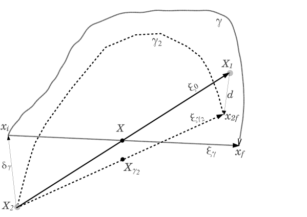
Figure 1: The points $X_{2}$ and $X_{1}$ have their mid point in $X$ and $\xi_{0}$ denotes the chord that joins them. The orbit $\gamma$, has also its center point in $X$ while its chord $\xi_{\gamma}^{t}$ joins the points $x_{i}$ and $x_{f}$. The orbit $\gamma$, starts in $x_{i}$ that is shifted from $X_{2}$ by the point shift $\delta_{\gamma}^{t}$. Meanwhile, orbit $\gamma_{2}$ starts in $X_{2}$ and evolves after a time $t$ up to $x_{2f}$, the drift from $X_{1}$ is denoted by $d^{t}$. For this last orbit $\gamma_{2}$, the chord is denoted by $\xi_{\gamma_{2}}^{t}$, while the mid point is $X_{\gamma_{2}}$. For simplicity, in the figure we have dropped the time superscripts $t$.

The chord $\xi_{\gamma}^{t}$ of the orbit $\gamma$ centered in $X$ is obtained by performing the derivative of the center generating function (33),

$$\xi_{\gamma}^{t}=-{\cal J}\frac{\partial S_{\gamma}^{t}(x)}{\partial x}\biggr{|}_{X}=\xi_{\gamma_{2}}^{t}-{\cal J}\mathit{B}_{t}\left(\xi_{0}-\xi_{\gamma_{2}}^{t}\right).$$

So that, recalling (22) , we get for the point shift

$$\delta_{\gamma}^{t}=\frac{1}{2}\left(\xi_{\gamma}^{t}-\xi_{0}\right)=\frac{1}{\mathcal{M}^{t}+1}d^{t},$$ (34)

where,

$$d^{t}=\xi_{\gamma_{2}}^{t}-\xi_{0}=x_{2f}-X_{1}$$ (35)

is the drift of the trajectory $\gamma_{2}$ that starting in $X_{2}$ ends up in $x_{2f}$ instead of $X_{1}$ (see Figure 1). In order to include the Morse index $\alpha_{\gamma_{2}}^{t}$ in the action let us define the action $\widetilde{S}_{\gamma_{2}}^{t}=S_{\gamma_{2}}^{t}+\hbar\frac{\pi}{2}\alpha_{\gamma_{2}}^{t}$. Hence, for the center action of the orbit $\gamma$ whose middle point is $X$ is we get

$$\widetilde{S}_{\gamma}^{t}(X) = \widetilde{S}_{\gamma_{2}}^{t}+\frac{1}{2}\xi_{\gamma_{2}}^{t}\wedge\xi_{0}+\frac{1}{4}d^{t\dagger}\mathit{B}_{t}d^{t}.$$ (36)

With expressions (36) and (34), respectively for the point shifts $\delta_{\gamma}^{t}$ and the center action $\widetilde{S}_{\gamma}^{t}(X)$, inserted in (32) we obtain for the coherent states propagator,

$$\langle X_{1}|\widehat{U}^{t}|X_{2}\rangle_{SC3}=\frac{2^{l}}{\left|\det\left[\mathcal{V}_{t}\left({\cal M}^{t}+1\right)\right]\right|^{\frac{1}{2}}}\exp\left[-\frac{d^{t\dagger}E_{t}d^{t}}{\hbar}\right]$$

$$\times\exp\frac{i}{\hbar}\left[\mathcal{S}_{2}^{t}+\left(\xi_{\gamma_{2}}^{t}+X\right)\wedge\frac{\xi_{0}}{2}+d^{t\dagger}\left(\frac{\mathit{B}_{t}}{4}+D_{t}\right)d^{t}\right].$$ (37)

Now $\varepsilon$ , the argument of $\det\left[\mathcal{V}_{t}\right]$ has been included in the action

$$\mathcal{S}_{2}^{t}=\widetilde{S}_{\gamma_{2}}^{t}+\hbar\frac{\varepsilon}{2}=S_{\gamma_{2}}^{t}+\hbar\frac{\pi}{2}\alpha_{\gamma_{2}}^{t}+\hbar\frac{\varepsilon}{2}$$

and the symmetric matrices $D_{t}$ and $E_{t}$ are defined as

$$D_{t} = \left(\frac{1}{\mathcal{M}^{t}+1}\right)^{\dagger}\mathcal{\overline{B}}_{t}\left(\frac{1}{\mathcal{M}^{t}+1}\right),$$

$$E_{t} = \left(\frac{1}{\mathcal{M}^{t}+1}\right)^{\dagger}\mathcal{\overline{C}}_{t}\left(\frac{1}{\mathcal{M}^{t}+1}\right)\textrm{ }.$$ (38)

Equation (37) is a general expression only in term of classical objects, its difference from (32) is that we have made use of the quadratic expansion of the action around the orbit $\gamma_{2}$ in order to express both the point shift $\delta_{\gamma}^{t}$ and the center generating function $\widetilde{S}_{\gamma}^{t}(X)$ of the orbit $\gamma$ only in terms of magnitudes given by the orbit $\gamma_{2}$ passing through $X_{2}$. This is a crucial advantage, now the semiclassical approximation of the CS matrix elements involves uniquely objects obtained directly by the classical evolution of the flux through $X_{2}$, namely, the chord $\xi_{\gamma_{2}}^{t}$ (or the drift $d^{t}$ defined in (35)), and the action $\mathcal{S}_{2}^{t}$ of the classical orbit $\gamma_{2}$ passing thorough $X_{2}$, and the monodromy matrix $\mathcal{M}^{t}$. From this former, equation (22) gives its Cayley representation $\mathit{B}_{t}$, after what, with (26), we get the complex matrix $\mathcal{V}_{t}$ while the real matrices $\mathcal{\overline{C}}_{t}$ and $\mathcal{\overline{B}}_{t}$ defined in (30) allows to obtain $D_{t}$ and $E_{t}$ through (38). Hence, there is no need for any further root search, neither integration over phase space conditions.

It is very useful to perform a comparison of the here derived Semiclassical CS propagator with other kinds of propagators based on Gaussian wave packets, namely the initial value representations (IVR) of the propagator. These propagators are generally based on wave packets of the form

$$\langle q|X^{\tau}\rangle=\left(\frac{\Re\tau}{\pi}\right)^{\frac{1}{4}}\exp\!\left[\!-\frac{\tau}{2}(q-Q)^{2}\!+\!i\frac{P}{\hbar}\left(q\!-Q\right)\!\right],$$

which resembles (1) if $\tau=\frac{m\omega}{\hbar}$. Although, the different phase factor ensures the symplectic invariance of the coherent states used in (1). In order to maintain the symplectic form we will then chose as in DE ,

$$\langle q|X^{\tau}\!\rangle\!=\!\left(\frac{\Re\tau}{\pi}\right)^{\frac{1}{4}}\!\!\exp\!\left[\!-\frac{\tau}{2}(q-Q)^{2}\!+\!i\frac{P}{\hbar}\left(q\!-\frac{Q}{2}\right)\!\right]\!.\!$$ (39)

With this choice, the overlap between two Gaussian wave packets is:

$$\langle X_{1}^{\tau_{1}}|X_{2}^{\tau_{2}}\rangle\!=\!\exp\!\left[-\frac{\left(X_{1}-X_{2}\right)^{2}}{4\hbar}\!-\!\frac{i}{2\hbar}X_{1}\wedge X_{2}\!\right],$$ (40)

the norm is defined as $X^{2}=X^{\dagger}\Lambda X$ where the symplectic squeezing matrix is

$$\Lambda=\left(\begin{array}[]{cc}\left(\hbar\sqrt{\tau_{1}\tau_{2}}\right)^{-1}&0\\ 0&\hbar\sqrt{\tau_{1}\tau_{2}}\end{array}\right).$$

The IVR of the propagator, in coordinates representation takes the form kay94 :

$$\!\!\!K^{t}(q,q^{\prime})\! \!\!=\! \langle q|\widehat{U}^{t}|q^{\prime}\rangle_{\!I\!V\!R\!}$$ (41)

$$\!\!\!\!=\!\!\!\! \!\!\!\int\!\!\!\frac{dX_{0}}{\left(2\pi\hbar\right)^{l}}\langle q|X_{t}^{\tau_{1}}\!\rangle R_{t}(\!X_{0}\!)e^{\frac{i}{\hbar}S^{t}\!(\!X_{0}\!)}\langle X_{0}^{\tau_{2}}\!|q^{\prime}\rangle,$$

where $\langle X_{0}^{\tau_{2}}|q^{\prime}\rangle$ is a Gaussian wave packet whose center lies in the point $X_{0}$ (initial point) in phase space. Meanwhile $\langle q|X_{t}^{\tau_{1}}\rangle$ is a Gaussian wave packet centered in the point $X_{t}$, that is the classically evolved initial point $X_{0}$ up to a time $t$. For the pre-exponential factor,

$$\!\!R_{t}(\!X_{0}\!)\!=\!\!\left[\!A\!\left(\!\!\tau_{1}m_{11}\!+\!\tau_{2}m_{22}\!-\!i\hbar\tau_{1}\tau_{2}m_{21}\!-\!\frac{1}{i\hbar}m_{12}\!\!\right)\!\right]^{\frac{1}{2}}\!,\!$$ (42)

where $A=\frac{1}{2\sqrt{\Re\tau_{1}\Re\tau_{2}}}$ and the monodromy matrix elements

$$\left(\begin{array}[]{c}\delta Q_{t}\\ \delta P_{t}\end{array}\right)=M\left(\begin{array}[]{c}\delta Q_{0}\\ \delta P_{0}\end{array}\right)=\left(\begin{array}[]{cc}m_{11}&m_{12}\\ m_{21}&m_{22}\end{array}\right)\left(\begin{array}[]{c}\delta Q_{0}\\ \delta P_{0}\end{array}\right)$$

connects the initial and final deviations of the trajectories $X_{t}$. While

$$S^{t}(X_{0})=\int_{0}^{t}\left[p{}_{t^{\prime}}\dot{q}{}_{t^{\prime}}-H\right]dt^{\prime}$$

is the classical action of the orbit that starts in $X_{0}$. The methods based on (41) are called initial value representation (IVR) and have shown to be very useful for many physical systems. They present the advantage over Van Vlek Gutwiller (VVG) VVleck ; gutz2 propagator that there is no need for any search of trajectories satisfying special boundary conditions.

Herman and Kluk (HK) formula is an IVR of the propagator that is also known as Frozen Gaussian Approximation (FGA) since in that case, the initial and final Gaussian have the same parameters $\tau_{1}=\tau_{2}=\tau$, a real positive constant. With this choice for the Gaussian parameters, the pre-factor (42) for the HK propagator is

$$\!R_{t}^{H\!K}\!(\!X_{0}\!)\!=\!\left|\!\frac{1}{2}\left(m_{11}\!+m_{22}-i\hbar\tau m_{21}-\frac{1}{i\hbar\tau}m_{12}\right)\!\right|\!^{\frac{1}{2}}\!,$$ (43)

that never vanishes. Hence the HK propagator is free of caustics singularities.

An also well known case of IVR is Heller’s Thawed Gaussian Approximation (TGA), where now the initial and final Gaussian parameters differ. While $\tau_{2}=\tau$ with again $\tau$ real positive,

$$\tau_{1}=-\frac{i}{\hbar}\frac{m_{12}+i\hbar\tau m_{11}}{m_{22}+i\hbar\tau m_{21}}$$

is complex. The prefactor (42) for this choice of parameters has now the form

$$\!R_{t}^{T\!G\!A}\!(\!X_{0}\!)\!=\!\left(\frac{\tau}{\Re\tau_{1}}\right)^{\frac{1}{4}}\left(m_{22}+i\hbar\tau m_{21}\right)^{-\frac{1}{2}}.$$ (44)

The IVR propagator can also be expressed in a mixed representation,

$$\!\!\!\!K^{t}(q,X_{2}) \!\!\!= \!\langle q|\widehat{U}^{t}|X_{2}\rangle_{I\!V\!R\!}=\int dq^{\prime}K^{t}(q,q^{\prime})\langle q^{\prime}|X_{2}\rangle\!$$ (45)

$$\!\!\!\!\!\!\!\!=\!\!\!\! \!\!\!\!\!\int\!\!\!\!\frac{dX_{0}}{\left(2\pi\hbar\right)^{l}}\!\langle q|\!X_{t}^{\tau_{1}}\rangle R_{t}\!(\!X_{0}\!)e^{\frac{i}{\hbar}S^{t}\!(\!X_{0}\!)}\langle X_{0}^{\tau_{2}}\!|X_{2}\rangle.$$

Note that we omit the $\tau$ superscript for the special case where $\tau=\frac{m\omega}{\hbar}$. The overlap between the wave functions can be performed analytically using (39) and (40), whereas the integration over initial phase space is still left over in the IVR propagator, but it is cut off by a bell shaped weight function (overlap between two Gaussians). One can perform this integration using Monte Carlo methods MC leading to a powerful numerical semiclassical procedure.

The HK propagator is a uniform semiclassical approximation of the exact propagator as has been shown by Kay kay . Indeed it is, the lowest order term of an expansion of the propagator in $\hbar$. Also, the HK propagator maintains unitarity for longer times than other IVR such as Heller’s TGA Harabati .

Although, as was stated by Grossmann and Herman in GH , a true HK-like expression must consist of an integration over initial phase space, which may not be treated in any additional approximation. However, it has been shown by Grossmann in comment that by a quadratic expansion of the exponent around the phase space center of the initial wavepacket, the TGA, originally derived by Heller in the mixed representation, can be obtained from the HK propagator, equation (45) with (43) and $\tau_{1}=\tau_{2}=\tau$.

Also, Baranger et al Baranger have shown that the TGA in the mixed representation is equivalent to their mixed propagator obtained with complex trajectories, except for two (related) differences. The presence of an extra phase that is associated with the use of the Gaussian averaged Hamiltonian $H$ in the computation of the action, rather than the Weyl symbol $H(x)$ (essentially the classical Hamiltonian$H_{C}$). In this respect, also Grossmann and Xavier GX have derived the HK propagator from the CS propagator proposed by Baranger el al. restricting themselves to real variables.

For the IVR of the propagator in the CS representation,

$$\!\!\!\!K^{t}(\!X_{1}\! \!, \!X_{2}\!)\!=\!\langle X_{1}|\widehat{U}^{t}|X_{2}\rangle_{I\!V\!R\!}\!=\!\int\!\!dq\langle X_{1}|q\rangle K^{t}(q,X_{2})\!$$ (46)

$$\!\!\!\!\!\!\!\!\!=\!\!\!\! \!\!\!\!\!\int\!\!\!\!\frac{dX_{0}}{\left(2\pi\hbar\right)^{l}}\!\langle X_{1}\!|X_{t}^{\tau_{1}}\rangle R_{t}\!(\!X_{0}\!)e^{\frac{i}{\hbar}S^{t}\!(\!X_{0}\!)}\langle X_{0}^{\tau_{2}}\!|X_{2}\rangle$$

the overlap between the Gaussians can be performed analytically, whereas, the phase space integration must be done numerically without any further approximation GH .

In this CS representation, Deshpande and Ezra DE found that expanding the exponent of the integrand in (46) up to quadratic terms and integrating , the linearized matrix element for the HK propagator conditions, they obtained an expression that is identical with Littlejohn form of the TGA matrix element little . Also, this expression resembles to the one obtained by Baranger et al Baranger except for the two differences previously described, that are related with the use of the Gaussian averaged Hamiltonian $H$, rather than the Weyl symbol $H(x)$.

A similar situation has been discussed by dos Santos and Aguiar aguiar , in order to obtain a CS path integral in the Weyl representation, who precisely argued the same difference with the representation used by Barranger et al. in Baranger . Indeed the expression obtained from the linearized HK propagator by Deshpande and Ezra in DE coincides with the expression given by dos Santos and Aguiar in aguiar . However, Deshpande and Ezra DE used real variables in their derivation not complex ones. This means that the linearized version of the HK propagator obtained in DE gives the expression (18) with real trajectories that is shown in section IV not to give accurate results. Hence, as was stated by Grossmann and Herman in GH , a true HK-like expression must consist of an integration over initial phase space, which may not be treated in any additional approximation.

On the other side, the expression (32) derived in this work is a semiclassical approximation that has been obtained directly from the semiclassical Weyl propagator. This last one, is the lowest order term of an expansion in $\hbar$, obtained through SPA but of the path integral expression of the propagator expressed in the Weyl representation, that is symplectically invariant. Only afterwards, the propagator is changed to the CS representation. For this last procedure, we avoid SPA, instead, we performed a quadratic expansion of the center action in the neighborhood of the relevant trajectories.

Then, the obtained expression (32) has the advantages of being a symplectically invariant expression only dealing with real trajectories. Also, differently from VVG propagators, it is free of caustic singularities. Although, it does not need any phase space integration, as is the case for IVR methods, the expression (32) has the drawback for the need of searching trajectories whose center lies in $X$. However, the quadratic expansion of the center action and its use as a generating function allowed us to obtain expression (37) that only involves objects relative to the orbit $\gamma_{2}$ passing though the initial point $X_{2}$.

IV Matrix elements for maps and application to the cat map

In what follows, we will obtain explicit expression for the classical objects involved in (37). In analogy with classical Poincaré surfaces of section. We will first perform the study on a surface of section that is transversal to the flux and passing through $X$. The flux restricted to this section is now a map on the section, for this map the time is discrete.

The study of autonomous fluxes through a map on surface of section is a standard procedure, in the case of billiards this is done through the well known Birkhoff coordinates. Also, quantum surface of section methods are shown to be exact prosen for general Hamiltonian systems. From now on, the $2l$ dimensional autonomous flux is studied through the $2l-2$ map on the mentioned surface of section.

As we have already mentioned, we need to evaluate the classical objects involved in (37). For that purpose, it will be convenient to express them in the basis of eigenvectors of the symplectic matrix. For the case of a map with one degree of freedom (corresponding to a two degrees of freedom flux), this is the stable and unstable vector basis $\left(\vec{\zeta_{u}},\vec{\zeta_{s}}\right)$ where the eigenvalues of the symplectic matrix $\mathcal{M}^{t}$ are $\exp(-\lambda t)$ and $\exp(\lambda t)$, ($\lambda$ is the stability or Lyapunov exponent of the orbit).

Let us then define $x_{s}$ and $x_{u}$ as canonical coordinates along the stable and unstable directions respectively such that $x=(x_{u},x_{s})=x_{u}\vec{\zeta_{u}}+x_{s}\vec{\zeta_{s}}$ with $\vec{\zeta_{u}}\wedge\vec{\zeta_{s}}=1$. As the basis formed by $\left(\vec{\zeta_{u}},\vec{\zeta_{s}}\right)$ is non orthonormal, the scalar product of two vectors takes the form,

$$x.y = x^{\dagger}\mathrm{\mathit{C}}y$$

$$= \left[\zeta_{u}^{2}x_{u}y_{u}+\zeta_{s}^{2}x_{s}y_{s}+\vec{\zeta_{u}}.\vec{\zeta_{s}}\left(x_{u}y_{s}+x_{s}y{}_{u}\right)\right].$$

That is, the scalar product matrix is,

$$\mathrm{\mathit{C}}=\left[\begin{array}[]{cc}\zeta_{u}^{2}&\vec{\zeta_{u}}.\vec{\zeta_{s}}\\ \vec{\zeta_{u}}.\vec{\zeta_{s}}&\zeta_{s}^{2}\end{array}\right]$$ (47)

with $\zeta_{u}^{2}=\vec{\zeta_{u}}.\vec{\zeta_{u}}$ and $\zeta_{s}^{2}=\vec{\zeta_{s}}.\vec{\zeta_{s}}$. Since the transformation from the orthonormal basis $\left(\vec{i},\vec{j}\right)$ to the basis $\left(\vec{\zeta_{u}},\vec{\zeta_{s}}\right)$ is symplectic

$$\det\mathit{C}=\zeta_{u}^{2}\zeta_{s}^{2}-\left(\vec{\zeta_{u}}.\vec{\zeta_{s}}\right)^{2}=1.$$

Also, in the $\left(\vec{\zeta_{u}},\vec{\zeta_{s}}\right)$ basis,

$$\mathcal{M}^{t}+1=2\cosh\left(\frac{\lambda t}{2}\right)\left[\begin{array}[]{cc}e^{t\nicefrac{{\lambda}}{{2}}}&0\\ 0&e^{-t\nicefrac{{\lambda}}{{2}}}\end{array}\right],$$ (48)

hence

$$\left|\det\left(\mathcal{M}^{t}+1\right)\right|=4\cosh^{2}\left(\frac{\lambda t}{2}\right),$$ (49)

is easily obtained only in terms of $\lambda$ and $t$. Analogously,

$$\mathcal{M}^{t}-1=2\sinh\left(\frac{\lambda t}{2}\right)\left[\begin{array}[]{cc}e^{t\nicefrac{{\lambda}}{{2}}}&0\\ 0&-e^{-t\nicefrac{{\lambda}}{{2}}}\end{array}\right],$$

while, $\mathit{B}_{t}$, the Cayley parametrization of $\mathcal{M}^{t}$, is in this basis

$$\mathit{B}_{t}=\left[\begin{array}[]{cc}0&\tanh\left(t\lambda/2\right)\\ \tanh\left(t\lambda/2\right)&0\end{array}\right].$$ (50)

Hence, using the expression of the symmetric matrix $\mathit{B}_{t}$ (50) and the scalar product (47) we get the complex matrix

$$\!\mathcal{V}_{t}\!=\!\mathit{C}\!-\!i\mathit{B}_{t}\!=\!\!\left[\!\!\begin{array}[]{cc}\zeta_{u}^{2}&\!\vec{\zeta_{u}}.\vec{\zeta_{s}}\!-\!i\tanh\left(\frac{t\lambda}{2}\right)\!\\ \!\vec{\zeta_{u}}.\vec{\zeta_{s}}\!-\!i\tanh\left(\frac{t\lambda}{2}\right)\!&\zeta_{s}^{2}\end{array}\!\!\right]\!.\!$$ (51)

Also, the complex determinant

$$\det\mathcal{V}_{t}=\left[1+\tanh^{2}\left(t\lambda/2\right)+2i\vec{\zeta_{u}}.\vec{\zeta_{s}}\tanh\left(t\lambda/2\right)\right],$$ (52)

with modulus

$$\!\left|\det\mathcal{V}_{t}\right|\!=\!\sqrt{\!\left[\!1+\tanh^{2}\!\left(\!\frac{t\lambda}{2}\!\right)\!\right]^{2}\!+\!\left[\!2\vec{\zeta_{u}}.\vec{\zeta_{s}}\tanh\!\left(\!\frac{t\lambda}{2}\!\right)\!\right]^{2}}\!$$ (53)

and argument

$$\epsilon=\arctan\frac{2\vec{\zeta_{u}}.\vec{\zeta_{s}}\tanh\left(t\lambda/2\right)}{1+\tanh^{2}\left(t\lambda/2\right)},$$ (54)

can be explicitly written in terms of the time and the Lyapunov exponent. Now, inverting the matrix $\mathcal{V}_{t}$ (51) we get,

$$\mathcal{V}_{t}^{-1} = \frac{-1}{\det\mathcal{V}_{t}}\left[\begin{array}[]{cc}-\zeta_{s}^{2}&\vec{\zeta_{u}}.\vec{\zeta_{s}}\!-\!i\tanh\left(\frac{t\lambda}{2}\right)\\ \!\vec{\zeta_{u}}.\vec{\zeta_{s}}\!-\!i\tanh\left(\frac{t\lambda}{2}\right)&-\zeta_{u}^{2}\end{array}\right]$$

$$= \frac{1}{\det\mathcal{V}_{t}}\left(\mathit{C}^{-1}+i\mathit{B}_{t}\right).$$

We must note that since the matrix $\mathcal{V}_{t}$ is symmetric, we get for the matrix $\mathcal{\widetilde{V}}$ defined in (30) that,

$$\mathcal{\widetilde{V}} = \frac{\mathcal{V}_{t}}{\det\mathcal{V}_{t}}=\frac{\left(\mathit{C}-i\mathit{B}_{t}\right)}{\left|\det\mathcal{V}_{t}\right|^{2}}\left(\Re(\mathbf{\det\mathcal{V}}_{t})-i\Im(\mathbf{\det\mathcal{V}}_{t})\right)$$ (56)

$$= \mathcal{\overline{C}}_{t}-i\mathcal{\overline{B}}_{t}.$$

Hence, in the stable and unstable vector basis $\left(\vec{\zeta_{u}},\vec{\zeta_{s}}\right)$, the real matrices $\mathcal{\overline{C}}_{t}$ and $\mathcal{\overline{B}}_{t}$ take the form

$$\mathcal{\overline{C}}_{t}=\frac{1}{\left|\det\mathcal{V}_{t}\right|^{2}}\left\{\mathit{C}th_{2}-2\mathit{B}_{t}\vec{\zeta_{u}}.\vec{\zeta_{s}}\tanh\left(\frac{t\lambda}{2}\right)\right\}$$ (57)

and

$$\mathcal{\overline{B}}_{t}=\frac{1}{\left|\det\mathcal{V}_{t}\right|^{2}}\left\{\mathit{B}_{t}th_{2}+2\mathit{C}\vec{\zeta_{u}}.\vec{\zeta_{s}}\tanh\left(\frac{t\lambda}{2}\right)\right\},$$ (58)

where $th_{2}=1+\tanh^{2}\left(\frac{t\lambda}{2}\right)$. The symmetric matrix $\mathit{B}_{t}$, the scalar product matrix $\mathit{C}$ and the determinant $\det\mathcal{V}_{t}$ are respectively given by the expressions (50), (47) and (53). Inserting the expressions (48), (57) and (58) in the definition of the symmetric matrices $D_{t}$ and $E_{t}$ (38), we get

$$D_{t}\!=\!\frac{-2\tanh\frac{t\lambda}{2}}{det_{1}}\!\left[\!\begin{array}[]{cc}\!-\!\zeta_{s}^{2}\!\left(\!\vec{\zeta_{u}}.\vec{\zeta_{s}}\!\right)\!e^{-\!t\lambda}&th_{2}\!+\!2\!\left(\vec{\!\zeta_{u}}.\vec{\zeta_{s}}\!\right)\!^{2}\\ th_{2}\!+\!2\!\left(\vec{\!\zeta_{u}}.\vec{\zeta_{s}}\!\right)\!^{2}&-\zeta_{u}^{2}\!\left(\!\vec{\zeta_{u}}.\vec{\zeta_{s}}\!\right)\!e^{t\lambda}\end{array}\!\right]$$ (59)

and

$$E_{t}=-\frac{th_{2}}{det_{1}}\left[\begin{array}[]{cc}-\zeta_{s}^{2}e^{-t\nicefrac{{\lambda}}{{2}}}&\frac{\vec{\zeta_{u}}.\vec{\zeta_{s}}}{2\sinh^{2}\left(t\lambda/2\right)+1}\\ \frac{\vec{\zeta_{u}}.\vec{\zeta_{s}}}{2\sinh^{2}\left(t\lambda/2\right)+1}&-\zeta_{u}^{2}e^{t\nicefrac{{\lambda}}{{2}}}\end{array}\right]$$ (60)

where we have defined

$$det_{1}=4\cosh^{2}\left(\frac{t\lambda}{2}\right)\left|\det\mathcal{V}_{t}\right|^{2}.$$

It is important to note that, (59), (60), (50), (52) and (49) are respectively explicit expression of the symmetric matrices $D_{t}$, $E_{t}$ and $\mathit{B}_{t}$ and the determinants $\left|\det\mathcal{V}_{t}\right|$and $\left|\det\left(\mathcal{M}^{t}+1\right)\right|$ for any value of the time $t$. Inserting these expressions in (37), we obtain a semiclassical expression for the matrix elements of the propagator in the CS basis entirely in terms of classical features such as, the chord $\xi_{0}$ that joins the points $X_{2}$ and $X_{1}$, the action of the orbit $\widetilde{S}_{X_{2}}$, the stable and unstable vectors $\vec{\zeta_{u}},\vec{\zeta_{s}}$ and the Lyapunov exponent $\lambda$.

Now the present theory is applied to the cat map i.e. the linear automorphism on the $2$-torus generated by the $2\times 2$ symplectic matrix $\mathcal{M}$, that takes a point $x_{-}$ to a point $x_{+}$ : $x_{+}=\mathcal{M}x_{-}\quad\mbox{mod(1)}$. In other words, there exists an integer $2$-dimensional vector $\mathbf{m}$ such that $x_{+}=\mathcal{M}x_{-}-\mathbf{m}$. Equivalently, the map can also be studied in terms of the center generating function mcat . This is defined in terms of center points

$$x\equiv\frac{x_{+}+x_{-}}{2}$$ (61)

and chords

$$\xi\equiv x_{+}-x_{-}=-\mathcal{J}\frac{\partial S(x,\mathbf{m})}{\partial x},$$ (62)

where

$$S(x,\mathbf{m}) =xBx+x\left(B-\mathcal{J}\right)\mathbf{m}+\frac{1}{4}\mathbf{m}(B+\widetilde{\mathcal{J}})\mathbf{m}$$ (63)

is the center generating function. Here $B$ is a symmetric matrix (the Cayley parameterization of $\mathcal{M}$, as in (50)), while

$$\widetilde{\mathcal{J}}=\left[\begin{array}[]{c|c}0&1\\ \hline\cr 1&0\end{array}\right].$$ (64)

We will study here the cat map with the symplectic matrix

$$\mathcal{\!M}\!=\!\left[\!\begin{array}[]{cc}2&3\\ 1&2\end{array}\!\right]\!\mbox{, and symmetric matrix }B\!=\!\left[\!\begin{array}[]{cc}-\frac{1}{3}&0\\ 0&1\end{array}\!\right]\!.\!$$ (65)

This map is known to be chaotic, (ergodic and mixing) as all its periodic orbits are hyperbolic. The map corresponds to viewing stroboscopically the motion generated by a quadratic Hamiltonian key-7 . However, the torus boundary conditions makes the dynamics as nonlinear as a dynamics can get key-7 . The eigenvalues of $\mathcal{M}$ are $e^{-\lambda}$ and $e^{\lambda}$ with $\lambda=\ln(2+\sqrt{3})\approx 1.317$. This is then the stability exponent for the fixed points, whereas the exponents must be doubled for orbits of period 2. All the eigenvectors have directions $\vec{\zeta_{s}}=(-\frac{\sqrt{3}}{2},\frac{1}{2})$ and $\vec{\zeta_{u}}=(1,\frac{1}{\sqrt{3}})$ corresponding to the stable and unstable directions respectively.

Quantum mechanics on the torus, implies a finite Hilbert space of dimension $N=\frac{1}{2\pi\hbar}$, and that positions and momenta are defined to have discrete values in a lattice of separation $\frac{1}{N}$ hanay ; opetor . The cat map was originally quantized by Hannay and Berry hanay in the coordinate representation the propagator is:

$$\langle\mathbf{q}_{k}|\hat{\mathbf{U}}_{\mathcal{M}}|\mathbf{q}_{j}\rangle=\left(\frac{i}{N}\right)^{\frac{1}{2}}{\exp}\left[\frac{i2\pi}{N}(k^{2}-jk+j^{2})\right],$$ (66)

where the states $\langle q|\mathbf{q}_{j}\rangle$ are periodic combs of Dirac delta distributions at positions $q=j/Nmod(1)$, with $j$ integer in $[0,N-1]$. In the Weyl representation opetor , the quantum map has been obtained in mcat as

$$\mathbf{U}_{\mathcal{M}}(x) =\frac{2}{\left|\det(\mathcal{M}+1)\right|^{\frac{1}{2}}}\sum_{\mathbf{m}}e^{i2\pi N\left[S(x,\mathbf{m})\right]}$$ (67)

where the center points are represented by $x=(\frac{a}{N},\frac{b}{N})$ with $a$ and $b$ integer numbers in $[0,N-1]$ for odd values of $N$ opetor . There exists an alternative definition of the torus Wigner function which also holds for even $N$.

The fact that the symplectic matrix $\mathcal{M}$ has equal diagonal elements implies in the time reversal symmetry and then the symmetric matrix $B$ has no off-diagonal elements. This property will be valid for all the powers of the map and, using (67), we can see that it implies in the quantum symmetry

$$\mathbf{U}_{\mathcal{M}}^{l}(p,q)=\left(\mathbf{U}_{\mathcal{M}}^{l}(-p,q)\right)^{*}=\left(\mathbf{U}_{\mathcal{M}}^{l}(p,-q)\right)^{*}.$$ (68)

for any integer value of $l$.

It has been shown hanay that the unitary propagator is periodic (nilpotent) in the sense that, for any value of $N$ there is an integer $k(N)$ such that

$$\hat{\mathbf{U}}_{\mathcal{M}}^{k(N)}=e^{i\phi}.$$

Hence the eigenvalues of the map lie on the $k(N)$ possible sites

$$\left\{\exp\left[\frac{i(2m\pi+\phi)}{k(N)}\right]\right\},\quad 1\leq m\leq k(N).$$ (69)

For the cases where $k(N)\langle N$ there are degeneracies and the spectrum does not behave as expected for chaotic quantum systems. In spite of the peculiarities in this map, a very weak nonlinear perturbations of cat maps restores the universal behavior of non degenerate chaotic quantum systems spectra matos . Eckhardt Eckhardt has argued that typically the eigenfunctions of cat maps are random.

The coherent states propagator on the torus depends on the definition of the periodic coherent state nonen , with $\langle p\rangle=P$ and $\langle q\rangle=Q$. In accordance to (1)

$$\langle{\bf X}|\mathbf{q}_{k}\rangle=\sum_{j=-\infty}^{\infty}e^{-\frac{1}{\hbar}\left[iP(j+\frac{Q}{2}-\nicefrac{{k}}{{N}})+\frac{1}{2}(j+Q-\nicefrac{{k}}{{N}})^{2}\right]}.$$ (70)

In order to construct operators or functions on the torus we have to periodize the construction. This is done merely using the recipe opetor that for any operator its Weyl representation on the torus ${\bf A}(x)$ is obtained from is analogue in the plane $A(x)$ by

$${\bf A}(x)=\sum_{j=-\infty}^{\infty}\sum_{k=-\infty}^{\infty}(-1)^{2ja+2kb+jkN}A(x+\frac{(k,j)}{2}).$$

Indeed the construction on the torus from the plane is obtain in terms of averages over equivalent points, that are obtained by translation with integer chords: $\widehat{T}_{\overrightarrow{k}}$ where $\overrightarrow{k}=\left(k_{p},k_{q}\right)$ is a two dimensional vector with integer components $k_{p}$ and $k_{q}$. Hence, the unit operator in the Hilbert space of the torus is opetor

$$\boldsymbol{\widehat{1}_{N}}=\sum_{k=0}^{N-1}|\mathbf{q}_{k}\rangle\langle\mathbf{q}_{k}|=\biggl{\langle}\widehat{T}_{\overrightarrow{k}}e^{i2\pi(\chi\wedge\overrightarrow{k}+\frac{N}{4}\overrightarrow{k}{\mathcal{\widetilde{J}}}\overrightarrow{k})}\biggr{\rangle}$$

so that

$$|{\bf X}\rangle = \boldsymbol{\widehat{1}_{N}}|X\rangle=\biggl{\langle}e^{i2\pi(\frac{N}{4}\overrightarrow{k}{\mathcal{\widetilde{J}}}\overrightarrow{k})}\widehat{T}_{\overrightarrow{k}}|X\rangle\biggr{\rangle}$$

$$= \biggl{\langle}e^{i\pi\frac{N}{2}\overrightarrow{k}{\mathcal{\widetilde{J}}}\overrightarrow{k}}e^{-\frac{i}{2\hbar}X\wedge\overrightarrow{k}}|X+\overrightarrow{k}\rangle\biggr{\rangle}.$$

In this way the coherent states matrix elements for any operator on the torus are obtained through

$$\langle\mathbf{X}_{1}|\mathbf{\widehat{A}}|\mathbf{X}_{2}\rangle\!=\!\biggl{\langle}\!e^{i\pi\frac{N}{2}\overrightarrow{k}{\mathcal{\widetilde{J}}}\overrightarrow{k}}e^{-\frac{i}{2\hbar}X\wedge\overrightarrow{k}}\langle X_{1}|\widehat{A}|X_{2}\!+\!\overrightarrow{k}\rangle\!\biggr{\rangle}.\!$$ (71)

Figure 2 shows the relative error $E$ on the amplitude of the semiclassical approximations $\langle X_{1}|\widehat{U}^{t}|X_{2}\rangle_{SC1}$ and $\langle X_{1}|\widehat{U}^{t}|X_{2}\rangle_{SC2}$ obtained respectively in (18) and (20) (after taking in both cases the torus periodization (71)) with respect to the exact expression obtained with the quantum propagator (66) on the CS (70). As can be seen, neither (18) nor (20) are good approximations of the exact CS matrix elements, giving errors in the amplitude of more than 10% or that highly grow with $N$ respectively. Meanwhile, we have verified that $\langle X_{1}|\widehat{U}^{t}|X_{2}\rangle_{SC3}$, obtained with (37), is exact in this case, for both the amplitude and the phase, as expected in a linear system.

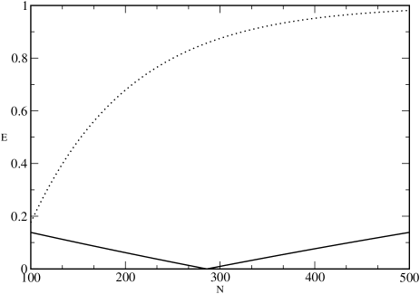
Figure 2: Relative error of the amplitude of the Semiclassical expressions $\langle X_{1}|\widehat{U}^{t}|X_{2}\rangle_{SC1}$ and $\langle X_{1}|\widehat{U}^{t}|X_{2}\rangle_{SC2}$ as a function of $N$. In full line the error of $\langle X_{1}|\widehat{U}^{t}|X_{2}\rangle_{SC1}$ and in dotted line the error of $\langle X_{1}|\widehat{U}^{t}|X_{2}\rangle_{SC2}$.

V Conclusions

To conclude, the expression (32) obtained in this work is an accurate semiclassical expression for the CS propagator that avoids complex trajectories, it only involves real ones. For its obtainment we have used the symplectically invariant Weyl representation. While the, semiclassical Weyl propagator was derived by performing a SPA for the path integral in the Weyl representation, for the transformation to CS representation SPA was avoided.

Also, the quadratic expansion of the center generating function has allowed to obtain a semiclassical expression of the CS propagator (37) involving only objects relative to the orbit $\gamma_{2}$ passing though the initial point $X_{2}$, without the need of any further search of trajectories that are typical procedures of Gutzwiller Van Vleck based propagators gutz2 ; VVleck , nor phase space integration typical from IVR methods.

For the case of chaotic maps, the explicit time dependence of the CS propagator has been derived only in terms of the action of the orbit through the initial point $X_{2}$, the Lyapunov exponent and the stable and unstable vector basis directions.

The comparison with a system whose semiclassical limit is exact has allowed to correctly check the exactness of expression (37) up to quadratic Hamiltonian systems.

It is important to mention that the present theory has already been successfully applied for the semiclassical matrix elements for chaotic propagators in the scar function basis scarelem . This is a crucial element in the semiclassical theory of short periodic orbits for the evaluation of the energy spectrum of classically chaotic Hamiltonian systems 6ver -13ver .

Of course, the here derived expression can be applied to a vast variety of systems, in particular for continuous Hamiltonian systems as was done with complex trajectories in ribeiro , indeed, the fact that only real trajectories are involved guaranties a simpler procedure.

I thanks G. Carlo, E. Vergini and M. Saraceno for stimulating discussions and the CONICET for financial support.

Appendix: Reflection Operators in Phase Space

Among the several representations of quantum mechanics, the Weyl-Wigner representation is the one that performs a decomposition of the operators that acts on the Hilbert space, on the basis formed by the set of unitary reflection operators. In this appendix we review the definition and some properties of this reflection operators.

First of all we construct the family of unitary operators

$$\hat{T}_{q}=\exp(-i\hbar^{-1}q.\hat{p}),\qquad\hat{T}_{p}=\exp(i\hbar^{-1}p.\hat{q}),$$ (72)

and following ozrep , we define the operator corresponding to a general translation in phase space by $\xi=(p,q)$ as

$$\hat{T}_{\xi} \equiv \exp\left(\frac{i}{\hbar}\xi\wedge\hat{x}\right)\equiv\exp\left[\frac{i}{\hbar}(p.\hat{q}-q.\hat{p})\right]$$ (73)

$$= \hat{T}_{p}\hat{T}_{q}\exp\left[-\frac{i}{2\hbar}\ p.q\right]\!=\!\hat{T}_{q}\hat{T}_{p}\exp\left[\frac{i}{2\hbar}\ p.q\right],$$ (74)

where naturally $\hat{x}=(\hat{p},\hat{q})$. In other words, the order of $\hat{T}_{p}$ and $\hat{T}_{q}$ affects only the overall phase of the product, allowing us to define the translation as above. $\hat{T}_{\xi}$ is also known as a Heisenberg operator. Acting on the Hilbert space we have:

$$\widehat{T}_{\xi}|q_{a}\rangle=e^{\frac{i}{\hbar}p(q_{a}+\frac{q}{2})}|q_{a}+q\rangle$$ (75)

and

$$\widehat{T}_{\xi}|p_{a}\rangle=e^{-\frac{i}{\hbar}q(p_{a}+\frac{p}{2})}|p_{a}+p\rangle.$$ (76)

We, hence, verify their interpretation as translation operators in phase space. The group property is maintained within a phase factor:

$$\hat{T}_{\xi_{2}}\hat{T}_{\xi_{1}}=\hat{T}_{\xi_{1}+\xi_{2}}e^{[\frac{-i}{2\hbar}\xi_{1}\wedge\xi_{2}]}=\hat{T}_{\xi_{1}+\xi_{2}}e^{[\frac{-i}{\hbar}D_{3}(\xi_{1},\xi_{2})]},$$ (77)

where $D_{3}$ is the symplectic area of the triangle determined by two of its sides. Evidently, the inverse of the unitary operator $\hat{T}_{\xi}^{-1}=\hat{T}_{\xi}^{{\dagger}}=\hat{T}_{-\xi}$ .

The set of operators corresponding to phase space reflections $\hat{R}_{x}$ about points $x=(p,q)$ in phase space, is formally defined in ozrep as the Fourier transform of the translation (or Heisenberg) operators

$$\widehat{R}_{x}\equiv(4\pi\hbar)^{-L}\int d\xi\quad e^{\frac{i}{\hbar}x\wedge\xi}\widehat{T}_{\xi}.$$ (78)

Their action on the coordinate and momentum bases are

$$\hat{R}_{x}\left|q_{a}\right\rangle = e^{2i(q-q_{a})p/\hbar}\;\left|2q-q_{a}\right\rangle$$ (79)

$$\hat{R}_{x}\left|p_{a}\right\rangle = e^{2i(p-p_{a})q/\hbar}\;\left|2p-p_{a}\right\rangle,$$ (80)

displaying the interpretation of these operators as reflections in phase space. Also, Using the coordinate representation of the coherent state (1) and the action of reflection on the coordinate basis (79), we can see that the action of the reflection operator $\widehat{R}_{x}$ on a coherent state $\left|X\right\rangle$ is the $x$ reflected coherent state

$$\widehat{R}_{x}\left|X\right\rangle=\exp\left(\frac{i}{\hbar}X\wedge x\right)\left|2x-X\right\rangle.$$ (81)

This family of operators have the property that they are a decomposition of the unity (completeness relation)

$$\hat{1}=\frac{1}{2\pi\hbar}\int dx\ \hat{R}_{x},$$ (82)

and also they are orthogonal in the sense that

$$Tr\left[\hat{R}_{x_{1}}\ \hat{R}_{x_{2}}\right]=2\pi\hbar\;\delta(x_{2}-x_{1}).$$ (83)

Hence, an operator $\hat{A}$ can be decomposed in terms of reflection operators as follows

$$\hat{A}=\frac{1}{2\pi\hbar}\int dx\ A_{W}(x)\ \hat{R}_{x}.$$ (84)

With this decomposition, the operator $\hat{A}$ is mapped on a function $A_{W}(x)$ living in phase space, the so called Weyl-Wigner symbol of the operator. Using (83) it is easy to show that $A_{W}(x)$ can be obtained by performing the following trace operation

$$A_{W}(x)=Tr\left[\hat{R}_{x}\ \hat{A}\right].$$

Of course, as it is shown in ozrep , the Weyl symbol also takes the usual expression in terms of matrix elements of $\hat{A}$ in coordinate representation

$$A_{W}(x)=\int\left\langle q-\frac{Q}{2}\right|\hat{A}\left|q+\frac{Q}{2}\right\rangle\exp\left(-\frac{i}{\hbar}pQ\right)dQ.$$

It was also shown in ozrep that reflection and translation operators have the following composition properties

$$\widehat{R}_{x}\widehat{T}_{\xi}=\widehat{R}_{x-\xi/2}e^{-\frac{i}{\hbar}x\wedge\xi}\ ,$$ (85)

$$\widehat{T}_{\xi}\widehat{R}_{x}=\widehat{R}_{x+\xi/2}e^{-\frac{i}{\hbar}x\wedge\xi}\ ,$$ (86)

$$\widehat{R}_{x_{1}}\widehat{R}_{x_{2}}=\widehat{T}_{2(x_{2}-x_{1})}e^{\frac{i}{\hbar}2x_{1}\wedge x_{2}}$$ (87)

so that

$$\widehat{R}_{x}\widehat{R}_{x}=\widehat{1}\ .$$ (88)

Now using (87) and (86) we can compose three reflections so that

$$\widehat{R}_{x_{2}}\widehat{R}_{x}\widehat{R}_{x_{1}}=e^{\frac{i}{\hbar}\Delta_{3}(x_{2},x_{1},x)}\widehat{R}_{x_{2}-x+x_{1}}$$ (89)

where $\Delta_{3}(x_{2},x_{1},x)=2(x_{2}-x)\wedge(x_{1}-x)$ is the area of the oriented triangle whose sides are centered on the points $x_{2},x_{1}$ and $x$ respectively.

References

• (1) E. Schrodinger, Naturwiss. 14, 664 (1926).
• (2) J.R. Klauder and B.S. Skagerstam, in Coherent states: Applications in Physics and Mathematical Physics, (Singapore: Word Scientific, 1985).
• (3) J.R. Klauder, “The Feynman Path Integral: An Historic Slice” in a “Garden of Quanta”, Eds. J. Arafune et al (Word Scientific, Singapore, 2003) , pp 55-77.
• (4) M.F. Herman and E. Kluk Chem. Phys. 91, 27 (1984).
• (5) W.H. Miller, Mol. Phys.100, 397 (2002).
• (6) J. Tatchen and E. Pollak, J. Chem. Phys. 130, 041103 (2009).
• (7) K.G. Kay, Chem. Phys. 322, 3 (2006).
• (8) K.G. Kay, J. Chem. Phys. 132, 244110 (2010).
• (9) M. Baranger , M. A. M. de Aguiar , F. Keck, H.J. Korsch and B. Schellhaaß, J. Phys. A: Math. Gen. 34, 7227 (2001). See also ibid 35, 9493 (2002) and references there in.
• (10) L.C. dos Santos and M.A.M. de Aguiar, J. Phys. A: Math. Gen. 39, 13465 (2006).
• (11) J. H. Wilson and V. Galitski, Phys. Rev. Lett. 106, 110401 (2011).
• (12) M.C. Gutzwiller in "Chaos and Quantum Physics", Les Houches Session LII, pg.205-248 Ed: M.-J. Giannonni, A. Voros and J. Zinn-Justin (1989).
• (13) J. H. V. Vleck, Proc. Natl. Acad. Sci. U.S.A. 14, 178 (1928).
• (14) A.M. Ozorio de Almeida, Physics Report 295, 266 (1998).
• (15) B. Mehlig and M. Wilkinson, Ann. Phys. (Leipzig) 10, 541-559 (2001).
• (16) M.V. Berry, Proc. R. Soc. A 423, 219 (1989).
• (17) K.G. Kay, J. Chem. Phys. 100, 4377 (1994).
• (18) C. Harabati, J.M. Rost and F. Grossmann, J. Chem. Phys. 120, 26 (2004).
• (19) F. Grossmann and M.F. Herman, J. Phys. A: Math. Gen. 35, 9489 (2002).
• (20) F. Grossmann, Comments At. Mol. Phys., 34, 141 (1999).
• (21) E. Kluk, M.F. Herman and H.L. Davis, J. Chem. Phys. 84, 326 (1986).
• (22) F. Grossmann and A.L. Xavier Jr., Phys. Lett. A 243, 243 (1998).
• (23) S.A. Deshpande and G.S. Ezra, J. Phys. A: Math. Gen. 39, 5067 (2006).
• (24) R.G. Littlejohn, Phys. Rep. 138, 193 (1986).
• (25) T. Prosen, J. Phys. A: Math. Gen. 28, 4133 (1995).
• (26) A.M.F. Rivas, M. Saraceno and A.M. Ozorio de Almeida, Nonlinearity 13, 341 (2000) .
• (27) J. P. Keating, Nonlinearity 4, 277 (1991).
• (28) J.H. Hannay and M.V. Berry, Physica D 1, 267 (1980).
• (29) A.M.F. Rivas and A.M. Ozorio de Almeida, Annals of Physics 276, 223 (1999).
• (30) M. Matos and A.M. Ozorio de Almeida, Annals of Physics 237, 46 (1995).
• (31) B. Eckhardt, J. Phys. A: Math. Gen. 19, 1823 (1986).
• (32) S. Nonnenmacher, Nonlinearity 10, 1569 (1997).
• (33) A.M.F. Rivas, J. Phys. A: Math. Gen. 46, 145101 (2013).
• (34) E. G. Vergini, J. Phys. A: Math. Gen., 33, 4709 (2000); E. G. Vergini and G. G. Carlo, J Phys. A: Math. Gen., 33, 4717 (2000).
• (35) D.A. Wisniacki, E.G. Vergini, R.M. Benito and F. Borondo, Phys. Rev. Lett. 94, 054101 (2005).
• (36) E. G. Vergini, D. Schneider and A. M. F. Rivas, J. Phys. A: Math. Theor. 41, 405102 (2008).
• (37) A.D. Ribeiro, M.A.M. de Aguiar, and M. Baranger, Phys. Rev. E. 69, 066204 (2004).