Asymmetric supernova in hierarchical multiple star systems and application to J1903+0327

Abstract

We develop a method to analyze the effect of an asymmetric supernova on hierarchical multiple star systems and we present analytical formulas to calculate orbital parameters for surviving binaries or hierarchical triples and runaway velocities for their dissociating equivalents. The effect of an asymmetric supernova on the orbital parameters of a binary system has been studied to great extent (e.g. Hills 1983; Kalogera 1996; Tauris & Takens 1998), but this effect on higher multiplicity hierarchical systems has not been explored before. With our method, the supernova effect can be computed by reducing the hierarchical multiple to an effective binary by means of recursively replacing the inner binary by an effective star at the center of mass of that binary. We apply our method to a hierarchical triple system similar to the progenitor of PSR J1903+0327 suggested by Portegies Zwart et al. (2011). We confirm their earlier finding that PSR J1903+0327 could have evolved from a hierarchical triple that became unstable and ejected the secondary star of the inner binary. Furthermore, if such as system did evolve via this mechanism the most probable configuration would be a small supernova kick velocity, an inner binary with a large semi-major axis, and the fraction of mass accreted onto the neutron star to the mass lost by the secondary would most likely be between 0.35 and 0.5

1 Introduction

Asymmetric supernovae (SNe) in binary and hierarchical multiple star systems form a crucial phase in the formation of stellar systems containing a compact stellar remnant - neutron star or black hole. In previous studies of SNe in binaries, two effects of the SN have been considered: (1) sudden mass loss and (2) a random kick velocity imparted on the compact remnant of the star undergoing the SN. The combined effect which changes the orbital parameters causes the binary to dissociate in the majority of the cases.

The study of binaries surviving a supernova (SN) explosion of one of its components was first performed by Blaauw (1961) and Boersma (1961), assuming a symmetric SN (i.e. only mass loss). The necessity of asymmetry in the SN, resulting in the kick velocity, was first suggested by Shklovskii (1970). The statistical study on pulsar scale heights by Gunn & Ostriker (1970) firmly supported the asymmetric SN model and to date the adding of the kick velocity to the newly born neutron star (or black hole) is a commonly excepted mechanism (van den Heuvel & van Paradijs 1997). Both the type of explosion mechanism and whether the exploding star is in a binary system are found to influence the effect of the kick velocity (see e.g. Podsiadlowski et al. 2004), but the exact physical process underlying the production of kicks remains unclear. The analysis of the effect of asymmetric supernovae on binaries has been sufficient to explain most of the observed post-SN stellar systems, and little to no effort has gone into studying the effect on hierarchical multiple star systems.

Millisecond pulsar (MSP) J1903+0327 (spin period $\simeq$ 2.15 ms), first observed by Champion et al. (2008) and later, in more detail, by Freire et al. (2011), is part of what may be the first observed MSP binary to have evolved from a hierarchical triple progenitor. MSP J1903+0327 is orbited by a main sequence star in a wide (orbital period $\simeq$ 95.2 days) and eccentric (eccentricity $e$ $\simeq$ 0.44) orbit. Based on these observables it seems impossible that this binary (hereafter J1903+0327) formed via the traditional mechanism in a binary progenitor (Champion et al. 2008). Portegies Zwart et al. (2011) proposed that the progenitor system was a binary accompanied by a third and least massive main-sequence star in a wider orbit about this binary. During the low-mass X-ray binary (LMXB) phase of the inner binary, the orbit of the LMXB expanded due to mass transfer from the evolving inner companion (donor) star to the neutron star, which was formed in the SN. This eventually caused the triple to become dynamically unstable and to eject the inner companion resulting in the observed system J1903+0327.

J1903+0327 is not a unique case, however: there is a significant number of systems like the progenitor of J1903+0327 as suggested in Portegies Zwart et al. (2011) and similar hierarchical stellar systems of higher multiplicity. The Multiple Star Catalog lists 602 triples, 93 quadruples, 22 quintuples, 9 sextuples and 2 septuples (Tokovinin 1997) of which 90 systems contain at least one star with a mass $M\geq 10$ M_⊙. Each of these multiples will eventually experience a core-collapse SN of the most massive star. After the SN these systems are either fully dissociated, dissociate into lower multiplicity multiple star systems, or survive the SN.

We begin the study of the effect of an asymmetric SN on hierarchical multiple star systems by first readdressing the SN effect on a binary and subsequently treating the effect in a hierarchical triple. We show that a hierarchical triple can effectively be regarded as a binary system comprised of the center of mass of the inner binary and the tertiary star. The effect of a SN on a hierarchical triple system, now reduced to an effective binary, can be calculated using the prescription for a SN in binary. We ultimately generalize this effective binary method to hierarchical multiple star systems of arbitrary multiplicity. In the second part of the paper we perform Monte Carlo simulations of a hierarchical triple star system similar to the progenitor of J1903+0327 suggested in Portegies Zwart et al. (2011) to determine the (stable) survival rates, and evaluate whether such a formation route is plausible.

2 Calculation of post-SN parameters

2.1 Binary systems

We consider a binary system of stars with mass, position and velocity for the primary and secondary star, given by ($m_{1,0}$,$\mathbf{r_{1}}$,$\mathbf{v_{1,0}}$) and ($m_{2}$,$\mathbf{r_{2}}$,$\mathbf{v_{2,0}}$) respectively, in which the primary undergoes a SN. The binary system is uniquely described by the semi-major axis, $a_{0}$, eccentricity, $e_{0}$, and true anomaly, $\theta_{0}$. The separation distance is $\mathbf{r_{0}}$. We assume that the SN is instantaneous, meaning an instantaneous removal of mass of the primary, no SN-shell impact on the companion (secondary) star, and the orbital motion during this mass loss phase is neglected, i.e. $\mathbf{r}=\mathbf{r_{0}}$ and $\mathbf{v_{2}}=\mathbf{v_{2,0}}$.

After the SN the orbital parameters have changed to: semi-major axis, $a$, eccentricity, $e$, and true anomaly, $\theta$. For a general Kepler orbit of two objects with masses $m_{1}$ and $m_{2}$ respectively, a relative velocity, $v$, semi-major axis, $a$, and separation distance, $r$, the orbital energy conservation equation is

$$v^{2}=G(m_{1}+m_{2})\Bigl{(}\frac{2}{r}-\frac{1}{a}\Bigr{)},$$ (1)

where $G$ is Newton’s gravitational constant. The specific relative angular momentum $\mathbf{h}$ is related to the orbital parameters as follows

$$|\mathbf{h}|^{2} = |\mathbf{r}\times\mathbf{v}|^{2}$$ (2)

$$= G(m_{1}+m_{2})a(1-e^{2}),$$ (3)

where the first equality holds for all Kepler orbits and the second only applies to bound orbits. For thorough studies on SNe in a binary system see Hills (1983), Kalogera (1996), and Tauris & Takens (1998); the latter authors also take into account the shell impact on the companion star using a method proposed by Wheeler, Lecar, & McKee (1975). Following the mentioned works as guides for our calculations on the binary system we use a total pre-SN mass of $M_{0}=m_{1,0}+m_{2}$. Without loss of generality, we choose a coordinate system in which at $t=0$ the orbit lies in the xy-plane, the center of mass of the binary (cm) is at the origin, the y-axis is the line connecting the primary and the secondary (the cm coordinate system; see Figure 1), and we choose a reference frame in which at $t=0$ the cm is at rest (the cm reference frame).

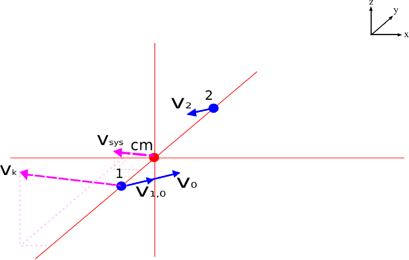
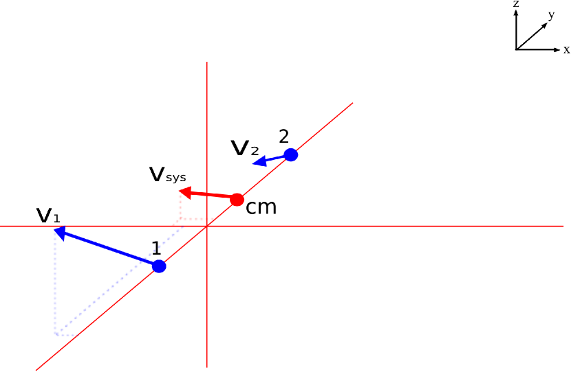
a. The cm coordinate system in the cm reference frame for a binary system before the SN (at $t=0$).   b. The cm coordinate system in the cm reference frame for a binary system after the SN.

Figure 1: Schematic representation of a binary system in the pre- and post-SN phase. The solid blue circles denote the primary and secondary star; the solid red cirle denotes the cm. The solid arrows denote the velocities the stars or cm have at that phase; the dashed arrows denote the velocity the SN imposes on the stars or cm which will change its velocity in the next phase. a. In the pre-SN phase the coordinate system is centered on the cm being at rest. b. In the post-SN phase the coordinate system is no longer centered on the cm - the cm has been translated in the y-direction, towards the secondary, and has gained a velocity $v_{sys}$. In both cases the inner binary orbital plane lies in the xy-plane and the y-axis is the line connecting the primary and the secondary.

Before the SN the separation distance between the stars is

$$\mathbf{r}=\mathbf{r_{1}}-\mathbf{r_{2}}=\left(0,-\frac{a_{0}(1-e_{0}^{2})}{1+e_{0}\cos\theta_{0}},0\right).$$ (4)

Using the following notation

$$x = a_{0}\sqrt{1-e_{0}^{2}}\cos\gamma_{0}\cos\theta_{0}+a_{0}\sin\gamma_{0}\sin\theta_{0},$$

$$y = -a_{0}\sqrt{1-e_{0}^{2}}\cos\gamma_{0}\sin\theta_{0}+a_{0}\sin\gamma_{0}\cos\theta_{0},$$

$$v_{0x} = v_{0}\frac{x}{\sqrt{x^{2}+y^{2}}},$$

$$v_{0y} = v_{0}\frac{y}{\sqrt{x^{2}+y^{2}}},$$

in which $\gamma_{0}$ is the pre-SN eccentric anomaly defined by $r=a_{0}(1-e_{0}\cos\gamma_{0})$, the velocity of the primary relative to the secondary is

$$\mathbf{v_{0}}=\mathbf{v_{1,0}}-\mathbf{v_{2}}=(v_{0x},v_{0y},0).$$ (5)

After the SN the primary has lost a part of its mass, $\Delta$m, and has obtained a velocity kick $\mathbf{v_{k}}$ in a random direction, which makes an angle $\phi$ with the pre-SN relative velocity $\mathbf{v_{0}}$. The velocity of the primary relative to the secondary, after the SN, is

$$\mathbf{v}=\mathbf{v_{0}}+\mathbf{v_{k}}=(v_{0x}+v_{kx},v_{0y}+v_{ky},v_{kz}),$$ (6)

the mass of the primary is $m_{1}=m_{1,0}-\Delta m$ and the total binary mass is $M=M_{0}-\Delta m$. Applying these relations and equations (1) and (2) to the binary system, we obtain equations relating the post-SN semi-major axis, $a$, and eccentricity, $e$, to both the pre- and post-SN orbital parameters and velocities. Using $v_{c,0}=v_{0}|_{r=a_{0}}=(GM_{0}/a_{0})^{1/2}$ as the pre-SN relative velocity (Hills 1983), we obtain

$$\frac{a}{a_{0}} = \Bigl{(}1-\frac{\Delta m}{M_{0}}\Bigr{)}\Bigl{(}1-\frac{2a_{0}}{r}\frac{\Delta m}{M_{0}}-2\frac{v_{0}}{v_{c,0}}\frac{v_{k}}{v_{c,0}}\cos\phi$$ (7)

$$-\frac{v_{k}^{2}}{v_{c,0}^{2}}\Bigr{)}^{-1}$$

$$e^{2} = 1-(1-e_{0}^{2})\frac{M_{0}^{2}}{(M_{0}-\Delta m)^{2}}\Bigl{(}1-\frac{2a_{0}}{r}\frac{\Delta m}{M_{0}}-\frac{v_{k}^{2}}{v_{c,0}^{2}}$$

$$-2\frac{v_{0}}{v_{c,0}}\frac{v_{k}}{v_{c,0}}\cos\phi\Bigr{)}$$

$$= 1-\frac{a_{0}^{2}(1-e_{0}^{2})^{2}}{a(1+e_{0}\cos\theta_{0})^{2}}\frac{(v_{0x}^{2}+v_{kx}^{2}+v_{kz}^{2}+2v_{0x}v_{kx})}{G(M_{0}-\Delta m)},$$

which are consistent with Kalogera (1996). In §2.3 we present a few examples regarding the effect of mass loss and the supernova kick on the orbital parameters of hierarchical triples. To compute the systemic velocity of the binary system due to the SN, we begin by writing the pre-SN velocities of the primary and secondary in the cm reference frame; using the pre-SN mass ratio $\mu_{0}=m_{2}/M_{0}$, these velocities are given by

$$\mathbf{v_{1,0}} = \mu_{0}\Bigl{(}v_{0x},v_{0y},0\Bigr{)},$$ (9)

$$\mathbf{v_{2}} = (\mu_{0}-1)\Bigl{(}v_{0x},v_{0y},0\Bigr{)}.$$ (10)

As a result of the assumption of an instantaneous SN and neglecting the shell impact, the instantaneous velocity of the secondary remains unchanged after the SN, but the instantaneous velocity of the primary changes to

$$\mathbf{v_{1}}=\Bigl{(}\mu_{0}v_{0x}+v_{kx},\mu_{0}v_{0y}+v_{ky},v_{kz}\Bigr{)}.$$ (11)

We now use the post-SN mass ratio $\mu=m_{2}/M$, and find the systemic velocity of the binary system:

$$\mathbf{v_{sys}} = (1-\mu)\mathbf{v_{1}}+\mu\mathbf{v_{2}}$$

$$= (1-\mu)\Bigl{(}\frac{\mu_{0}-\mu}{1-\mu}v_{0x}+v_{kx},\frac{\mu_{0}-\mu}{1-\mu}v_{0y}+v_{ky},v_{kz}\Bigr{)}.$$

These results are consistent with the previously mentioned studies on SN in binaries. As a conseqence a binary in which the compact object does not receive a kick in the supernova explosion moves through space like a frisbee.

2.1.1 Dissociating binary systems

The mass loss and the kick velocity have a potentially disrupting effect on the binary system. However, in cases where the mass loss alone would have been large enough to unbind the binary, the combination of the two can result in the binary system surviving the SN (Hills 1983). If the binary system dissociates, the two stars move away from each other on a hyperbolic or, in a limiting case, a parabolic trajectory. This corresponds to the cases where $a<0$ and $e>1$ (hyperbola) or $a\to\infty$ and $e=1$ (parabola). From equation (7) we see that for a dissociating binary the angle $\phi$ between the kick velocity $\mathbf{v_{k}}$ and the pre-SN relative velocity $\mathbf{v_{0}}$ satisfies (Hills 1983):

$$\cos\phi \geq \Bigl{(}1-\frac{2a_{0}}{r}\frac{\Delta m}{M_{0}}-\frac{v_{k}^{2}}{v_{c,0}^{2}}\Bigr{)}\Bigl{(}2\frac{v_{k}}{v_{c,0}}\sqrt{\frac{2a_{0}}{r}-1}\Bigr{)}^{-1}.$$ (13)

If the right-hand side of equation (13) is less than $-1$, the binary dissociates for all $\phi$; but if it is greater than $1$ the binary survives for all $\phi$. If the right-hand side is within the range $-1$ to $1$, the probability of dissociating the binary is (Hills 1983):

$$P_{diss} = \frac{1}{2}\Bigl{(}1-\Bigl{(}1-\frac{2a_{0}}{r}\frac{\Delta m}{M_{0}}-\frac{v_{k}^{2}}{v_{c,0}^{2}}\Bigr{)}\Bigl{(}2\frac{v_{0}}{v_{c,0}}\frac{v_{k}}{v_{c,0}}\Bigr{)}^{-1}\Bigr{)}.$$

Tauris & Takens (1998) presented analytical formulas to calculate the dissociation velocities for a binary with a pre-SN circular orbit. We follow Tauris & Takens’ calculations, though ignore the SN shell impact, to derive the runaway velocities of two stars in dissociating binaries, however we do so for a pre-SN orbit with arbitrary eccentricity. We use the cm coordinate system, explained above. Using the following shorthand relations

$$\tilde{m} = \frac{M}{M_{0}},$$

$$j = \frac{v_{0x}^{2}}{v_{0}^{2}}-2\tilde{m}\frac{a_{0}}{2a_{0}-r}+\frac{v_{k}^{2}}{v_{0}^{2}}+\frac{2v_{0x}v_{kx}}{v_{0}^{2}},$$

$$k = 1+\frac{j}{\tilde{m}}\frac{2a_{0}-r}{a_{0}}-\frac{v_{ky}^{2}}{\tilde{m}v_{0}^{2}}\frac{2a_{0}-r}{a_{0}},$$

$$l = \frac{1}{\mu}\Bigl{(}\frac{\sqrt{j}}{\tilde{m}v_{0}}v_{ky}\frac{2a_{0}-r}{a_{0}}-\frac{j}{\tilde{m}}\frac{2a_{0}-r}{a_{0}}-1\Bigr{)},$$

$$n = \frac{1}{\mu}\Bigl{(}1+\frac{j}{\tilde{m}}\frac{2a_{0}-r}{a_{0}}(k+1)\Bigr{)},$$

we find the runaway velocities for the primary and secondary star:

$$\mathbf{v_{1,diss}} = \Bigl{(}v_{kx}\Bigl{(}\frac{1}{l}+1\Bigr{)}+\Bigl{(}\frac{1}{l}+\mu_{0}\Bigr{)}v_{0x},\mu_{0}v_{0y}$$ (15)

$$+v_{ky}\Bigl{(}1-\frac{1}{n}\Bigr{)}+\frac{k\sqrt{j}}{n}v_{0},v_{kz}\Bigl{(}\frac{1}{l}+1\Bigr{)}\Bigr{)},$$

$$\mathbf{v_{2,diss}} = \Bigl{(}-\frac{v_{kx}}{m_{2}l}-\Bigl{(}\frac{1}{m_{2}l}+1-\mu_{0}\Bigr{)}v_{0x},(\mu_{0}-1)v_{0y}$$ (16)

$$+\frac{v_{ky}}{m_{2}n}-\frac{k\sqrt{j}}{m_{2}n}v_{0},-\frac{v_{kz}}{m_{2}l}\Bigr{)}.$$

2.2 Hierarchical triple systems

We now consider a hierarchical system of three stars with the primary, secondary and tertiary star having mass, position and velocity given by ($m_{1,0}$,$\mathbf{r_{1}}$,$\mathbf{v_{1,0}}$), ($m_{2}$,$\mathbf{r_{2}}$,$\mathbf{v_{2}}$) and ($m_{3}$,$\mathbf{r_{3}}$,$\mathbf{v_{3}}$) respectively. The primary star undergoes a SN and the inner binary configuration and parameters are the same as in section 2.1. The effective mass of the inner binary’s centre of mass (cm) is $m_{cm,0}=m_{1,0}+m_{2}=M_{0}$, and is at position

$$\mathbf{r_{cm,0}}=(1-\mu_{0})\mathbf{r_{1}}+\mu_{0}\mathbf{r_{2}}$$ (17)

and has a velocity

$$\mathbf{v_{cm,0}}=(1-\mu_{0})\mathbf{v_{1,0}}+\mu_{0}\mathbf{v_{2}}.$$ (18)

The cm and tertiary constitute an outer binary defined by the semi-major axis, $A_{0}$, eccentricity, $E_{0}$, and true anomaly, $\Theta_{0}$. The separation distance between the cm and the tertiary star we denote by $\mathbf{R_{0}}$. Before the SN the outer binary orbital plane has an inclination $i_{0}$ with respect to the inner binary and the separation distance of the outer binary projected onto the xy-plane makes an angle $\alpha_{0}$ with the separation distance of the inner binary. This inner-outer binary configuration is to some extent acceptable, because the triple is hierarchical. This implies that the separation distance of the cm and the tertiary is large compared to the separation distance of the primary and secondary, i.e. $R_{0}\gg r_{0}$, so that the tertiary experiences gravitational influence of the inner binary as if it was coming from one star at the cm. We assume an instantaneous SN. Due to the primary undergoing a SN, the inner binary experiences a mass loss $\Delta m$ and an effective kick velocity is imparted to the cm: the systemic velocity of the inner binary $\mathbf{v_{sys}}$ given by equation 2.1. In addition, because of the reduction in mass of the primary, the position of the cm has changed due to an instantaneous translation along the y-axis

$$\mathbf{\Delta R} = \mathbf{r_{cm}}-\mathbf{r_{cm,0}}$$ (19)

$$= (\mu-\mu_{0})\frac{a_{0}(1-e_{0}^{2})}{1+e_{0}\cos\theta_{0}}\Bigl{(}0,1,0\Bigr{)}.$$

The orbital parameters change as a result of the SN: the inner binary parameters change according to the description in section 2.1 and the outer binary orbital parameters change to semi-major axis, $A$, eccentricity, $E$, and true anomaly, $\Theta$. The hierarchical triple before the SN has a total mass $M_{t,0}=M_{0}+m_{3}$. We use the cm coordinate system to pin down the inner binary and add to this coordinate system the tertiary at a position such that $R_{0}\gg r_{0}$ (see Figure 2). We now select a reference frame in which the center of mass of the triple (CM) is at rest (the CM reference frame).

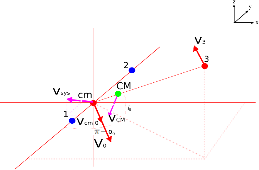
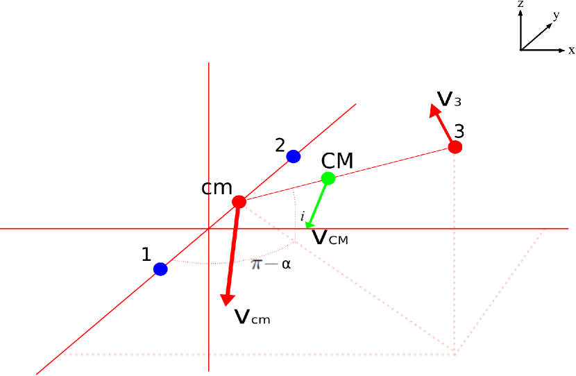
a. The cm coordinate system in the CM reference frame for a hierarchical triple system before the SN (at $t=0$).   b. The cm coordinate system in the CM reference frame for a hierarchical triple system after the SN.

Figure 2: Schematic representation of a hierarchical triple star system in the pre- and post-SN phase. The solid blue circles denote the primary and secondary (inner binary); the solid red cirles denote the cm and the tertiary (outer binary); the green cirle denotes the CM. The solid arrows denote the velocities the stars or cm have at that phase; the dashed arrows denote the velocity the SN imposes on the stars or cm which will change its velocity in the next phase. (a) In the pre-SN phase at the moment immediately preceding the SN, the coordinate system is centered on cm and CM is at rest. (b) In the post-SN phase the coordinate system is no longer centered on the cm - the cm has been translated in the y-direction, towards the secondary - and the CM is no longer at rest. In both cases the inner binary orbital plane lies in the xy-plane and the y-axis is the line connecting the primary and the secondary.

Prior to the SN the separation distance between the cm and the tertiary is

$$\mathbf{R_{0}}=\frac{A_{0}(1-E_{0}^{2})}{1+E_{0}\cos\Theta_{0}}\Bigl{(}\cos i_{0}\sin\alpha_{0},-\cos i_{0}\cos\alpha_{0},\sin i_{0}\Bigr{)},$$ (20)

and, using the following shorthand notation

$$X = A_{0}\sqrt{1-E_{0}^{2}}\cos\Gamma_{0}\cos\Theta_{0}+A_{0}\sin\Gamma_{0}\sin\Theta_{0}$$

$$Y = -A_{0}\sqrt{1-E_{0}^{2}}\cos\Gamma_{0}\sin\Theta_{0}+A_{0}\sin\Gamma_{0}\cos\Theta_{0}$$

$$X^{\prime} = X\cos\alpha_{0}-Y\cos i_{0}\sin\alpha_{0}$$

$$Y^{\prime} = X\sin\alpha_{0}+Y\cos i_{0}\cos\alpha_{0}$$

$$Z^{\prime} = Y\sin i_{0}$$

$$V_{0x} = V_{0}\frac{X^{\prime}}{\sqrt{X^{\prime 2}+Y^{\prime 2}+Z^{\prime 2}}}$$

$$V_{0y} = V_{0}\frac{Y^{\prime}}{\sqrt{X^{\prime 2}+Y^{\prime 2}+Z^{\prime 2}}}$$

$$V_{0z} = V_{0}\frac{Z^{\prime}}{\sqrt{X^{\prime 2}+Y^{\prime 2}+Z^{\prime 2}}}$$

in which $\Gamma_{0}$ is the pre-SN outer orbit eccentric anomaly defined by $R_{0}=A_{0}(1-E_{0}\cos\Gamma_{0})$, the velocity of the cm relative to the tertiary is

$$\mathbf{V_{0}}=\mathbf{v_{cm,0}}-\mathbf{v_{3}}=(V_{0x},V_{0y},V_{0z}).$$ (21)

The effective kick velocity $\mathbf{v_{sys}}$ makes an angle $\Phi$ with the pre-SN relative velocity of the cm with respect to the tertiary star $\mathbf{V_{0}}$. After the SN the separation distance between the cm and the tertiary star is

$$\mathbf{R} = \mathbf{R_{0}}+\mathbf{\Delta R},$$ (22)

$$= \frac{A_{0}(1-E_{0}^{2})}{1+E_{0}\cos\Theta_{0}}\Bigl{(}\cos i_{0}\sin\alpha_{0},(\mu-\mu_{0})\frac{a_{0}(1-e_{0}^{2})}{1+e_{0}\cos\theta_{0}}$$

$$\times\frac{1+E_{0}\cos\Theta_{0}}{A_{0}(1-E_{0}^{2})}-\cos i_{0}\cos\alpha_{0},\sin i_{0}\Bigl{)},$$

the velocity of the cm relative to the tertiary star is

$$\mathbf{V} = \mathbf{V_{0}}+\mathbf{v_{sys}}$$ (23)

$$= (V_{0x}+v_{sys,x},V_{0y}+v_{sys,y},V_{0z}+v_{sys,z}),$$

the cm mass is $m_{cm}=M_{0}-\Delta m$ and the total triple mass is $M_{t}=M_{t,0}-\Delta m$. The inclination of the outer binary orbital plane with respect to the inner binary orbital plane is given by:

$$\sin i=\frac{|\mathbf{R_{0}}|}{|\mathbf{R}|}\sin i_{0}.$$ (24)

The angle of the outer binary separation distance projected onto the xz-plane relative to the inner binary separation distance is given by:

$$\sin\alpha=\frac{|\mathbf{R_{0}}|}{|\mathbf{R}|}\frac{\cos i_{0}}{\cos i}\sin\alpha_{0}.$$ (25)

Applying the relevant equations above and equations (1) and (2) to our triple system, we obtain equations relating the post-SN semi-major axis, $A$, and eccentricity, $E$, to both the pre- and post-SN orbital parameters and velocities. Using $V_{c,0}=V_{0}|_{R_{0}=A_{0}}=(GM_{t,0}/A_{0})^{1/2}$ as the pre-SN relative velocity when $R_{0}=A_{0}$, and using $\rho=(R_{0}-R)/(R_{0}R)$, we obtain

$$\frac{A}{A_{0}} = \Bigl{(}1-\frac{\Delta m}{M_{t,0}}\Bigr{)}\Bigl{(}1-\frac{2A_{0}}{R}\frac{\Delta m}{M_{t,0}}-2\frac{V_{0}}{V_{c,0}}\frac{v_{sys}}{V_{c,0}}\cos\Phi$$ (26)

$$-\frac{v_{sys}^{2}}{V_{c,0}^{2}}+2A_{0}\rho\Bigr{)}^{-1},$$

$$E^{2} = 1-(1-E_{0}^{2})\frac{M_{t,0}}{(M_{t,0}-\Delta m)}\Bigl{(}\frac{2A_{0}}{R}+\frac{M_{t,0}}{M_{t,0}-\Delta m}$$

$$\times\Bigl{(}1-\frac{2A_{0}}{R_{0}}-\frac{v_{sys}^{2}}{V_{c,0}^{2}}-2\frac{V_{0}}{V_{c,0}}\frac{v_{sys}}{V_{c,0}}\cos\Phi\Bigr{)}\Bigr{)}.$$

With the pre-SN mass ratio $\nu_{0}=m_{3}/M_{t,0}$, the pre-SN velocities of the cm and the tertiary in the CM reference frame are

$$\mathbf{v_{cm,0}} = \nu_{0}\Bigl{(}V_{0x},V_{0y},V_{0z}\Bigr{)}$$ (28)

$$\mathbf{v_{3}} = (\nu_{0}-1)\Bigl{(}V_{0x},V_{0y},V_{0z}\Bigr{)}.$$ (29)

We calculate the instantaneous velocity of the cm after the SN (as before, because of the assumption of an instantaneous SN, the velocity of the tertiary after the SN remains unchanged):

$$\mathbf{v_{cm}}=\nu_{0}\Bigl{(}V_{0x}+\frac{v_{sys,x}}{\nu_{0}},V_{0y}+\frac{v_{sys,y}}{\nu_{0}},V_{0z}+\frac{v_{sys,z}}{\nu_{0}}\Bigr{)}.$$ (30)

Using the post-SN mass ratio $\nu=m_{3}/M_{t}$, the systemic velocity of the outer binary (and therefore of the triple) is

$$\mathbf{V_{sys}} = (1-\nu)\mathbf{v_{cm}}+\nu\mathbf{v_{3}}$$ (31)

$$= (1-\nu)\Bigl{(}\frac{\nu_{0}-\nu}{1-\nu}V_{0x}+(\mu_{0}-\mu)v_{0x}+(1-\mu)v_{kx},$$

$$\frac{\nu_{0}-\nu}{1-\nu}V_{0y}+(\mu_{0}-\mu)v_{0y}+(1-\mu)v_{ky},$$

$$\frac{\nu_{0}-\nu}{1-\nu}V_{0z}+(1-\mu)v_{kz}\Big{)}.$$

Summarizing, one can consider a hierarchical triple system as a effective binary system composed of an effective star (i.e. the inner binary center of mass (cm)) and the tertiary. The effective star undergoes an effective asymmetric SN resulting in three effects: 1) sudden mass loss $\Delta m$, 2) an instantaneous translation $\mathbf{\Delta R}$, and 3) a random kick velocity $\mathbf{v_{sys}}$. The calculation of the post-SN parameters and velocities of a hierarchical triple system is now reduced to the prescription for a SN in a binary as presented in section 2.1. Note that the mass loss does not occur from the position of the effective star, but from the position of the primary star; a clear distinction from a physical binary system. However, from what position the mass loss occurs is not important when an instantaneous SN is considered. When the effect of the shell impact on the companion star(s) is considered, this off-center mass loss must be taken into account. In addition, if it were not the primary which underwent the SN, but, for example, the tertiary, the computation would have been done by reducing the inner binary to an effective star, as shown in this section. One would again have a binary configuration to calculate the effect of the SN; in such a system there is no off-center mass loss. In section 2.4 we show how one can reduce any hierarchical multiple star system to an effective binary in a recursive way using the effective binary method and in §  2.4.3 we do the computation of the effect of a SN on a binary-binary system.

2.2.1 Dissociating hierarchical triple systems

For the triple system, dissociation can occur in two ways: the inner binary can dissociate ($a<0$ and $e>1$ or $a\to\infty$ and $e=1$) (see section 2.1) and the outer binary can dissociate ($A<0$ and $E>1$ or $A\to\infty$ and $E=1$), i.e. the inner binary and the tertiary become unbound. The inner binary dissociation scenario generally results in complete dissociation of the system. However, hypothetical scenarios exist in which one of the inner binary components is ejected towards the tertiary star to either collapse with it or to form a binary by gravitational or tidal capture. Nevertheless, these scenarios have a small probability since the ejection conditions (e.g. the solid angle in which that particular inner binary component has to be ejected in) and the capture conditions are extremely specific. From equation 26 we see that for the inner binary to dissociate from the tertiary, the angle $\Phi$ has to satisfy

$$\cos\Phi \geq \Bigl{(}1-\frac{2A_{0}}{R}\frac{\Delta m}{M_{t,0}}-\frac{v_{sys}^{2}}{V_{c,0}^{2}}+2A_{0}\rho\Bigr{)}\Bigl{(}2\frac{V_{0}}{V_{c,0}}\frac{v_{sys}}{V_{c,0}}\Bigr{)}^{-1}.$$

The probability of this type of dissociation is

$$P_{diss}^{outer} = \frac{1}{2}\Bigl{(}1-\Bigl{(}1-\frac{2A_{0}}{R}\frac{\Delta m}{M_{t,0}}-\frac{v_{sys}^{2}}{V_{c,0}^{2}}+2A_{0}\rho\Bigr{)}$$ (33)

$$\times\Bigl{(}2\frac{V_{0}}{V_{c,0}}\frac{v_{sys}}{V_{c,0}}\Bigr{)}^{-1}\Bigr{)}.$$

In the case of the dissociation of the outer binary, using the following short hand relations

$$\tilde{M} = \frac{M_{t}}{M_{t,0}}$$

$$J = \frac{V_{0x}^{2}}{V_{0}^{2}}-2\tilde{M}\frac{A_{0}}{2A_{0}-R_{0}}\frac{R_{0}}{R}+\frac{v_{sys}^{2}}{V_{0}^{2}}+\frac{2V_{0x}v_{sys,x}}{V_{0}^{2}}$$

$$K = 1+\frac{J}{\tilde{M}}\frac{2A_{0}-R_{0}}{A_{0}}\frac{R}{R_{0}}-\frac{v_{sys,y}^{2}}{\tilde{M}V_{0}^{2}}\frac{2A_{0}-R}{A_{0}}\frac{R}{R_{0}}$$

$$L = \frac{1}{\nu}\Bigl{(}\frac{\sqrt{J}}{\tilde{M}V_{0}}v_{sys,y}\frac{2A_{0}-R_{0}}{A_{0}}\frac{R}{R_{0}}$$

$$-\frac{J}{\tilde{M}}\frac{2A_{0}-R_{0}}{A_{0}}\frac{R}{R_{0}}-1\Bigr{)}$$

$$N = \frac{1}{\nu}\Bigl{(}1+\frac{J}{\tilde{M}}\frac{2A_{0}-R_{0}}{A_{0}}\frac{R}{R_{0}}(K+1)\Bigr{)}$$

the runaway velocities of the inner binary system and the tertiary are (following and generalizing Tauris & Takens (1998)):

$$\mathbf{v_{cm,diss}} = \Bigl{(}v_{sys,x}\Bigl{(}\frac{1}{L}+1\Bigr{)}+\Bigl{(}\frac{1}{L}+\nu_{0}\Bigr{)}V_{0x},v_{sys,y}\Bigl{(}1-\frac{1}{N}\Bigr{)}$$ (34)

$$+\nu_{0}V_{0y}+\frac{K\sqrt{J}}{N}V_{0},v_{sys,z}\Bigl{(}\frac{1}{L}+1\Bigr{)}\Bigr{)}$$

$$\mathbf{v_{3,diss}} = \Bigl{(}-\frac{v_{sys,x}}{m_{3}L}-\Bigl{(}\frac{1}{m_{3}L}+1-\nu_{0}\Bigr{)}V_{0x},(\nu_{0}-1)V_{0y}$$ (35)

$$+\frac{v_{sys,y}}{m_{3}N}-\frac{K\sqrt{J}}{m_{3}N}V_{0},-\frac{v_{sys,z}}{m_{3}L}\Bigr{)}.$$

Note that these equations are more general than the ones in section 2.1.1, because we cannot assume $\mathbf{R}=\mathbf{R_{0}}$ in the triple case.

2.3 An example of the effect of a supernova in a hierarchical triple

For two simple sets of initial conditions we investigated the effect of mass loss, $\Delta m$, and kick velocity, $\mathbf{v_{k}}$, on the survivability of a triple system. We distinguish between four different post-SN scenarios: (1) the triple survives as a whole ($e<1$ and $E<1$) with new orbital parameters, (2) the inner binary survives and the third star escapes ($e<1$ and $E>1$), (3) the inner binary dissociates and the outer binary survives ($e>1$ and $E<1$) and (4) the triple completely dissociates ($e>1$ and $E>1$). The third scenario is a rather special case and can only be of temporary nature: in this scenario, even though the inner binary has just dissociated, the third star remains bound to the inner binary center of mass. This is a temporal solution which eventually will lead to the full dissociation of the triple, except in the extreme case in which the tertiary star captures one of the ejected inner stars to form a new binary system.

For each set of initial conditions we used a hierarchical triple system with primary, secondary and tertiary stars of masses m_1,0, m₂, m₃ = 3, 2, 1 M_⊙ respectively and inner and outer binary semi-major axes a₀, A₀ = 10, 50 R_⊙ respectively, and we varied the kick velocity direction $\mathbf{\hat{v}_{k}}$. For the two different sets of initial conditions we determine which combinations of $\Delta m$ and $v_{k}$ lead to which post-SN scenario and we show our results in Figure 3; the used initial conditions are specified below the respective figures.

In Figure 3a. we used a circular inner and outer orbit, not inclined with respect to each other, with all stars on one line and the kick velocity in the same direction as the pre-SN inner binary relative velocity. We see that for zero kick velocity, the inner binary dissociates for a mass loss ratio of $\Delta m/M_{0}=0.5$, which is consistent with earlier work (e.g. Hills 1983). For zero mass loss, we see that the inner binary dissociates for a kick velocity of $\mathbf{v_{k}}\sim 128$ km/s - this velocity is exactly the difference between the inner binary escape velocity (v${}_{esc}=\sqrt{2GM_{0}/a_{0}}\sim 437$ km/s) and pre-SN relative velocity (v${}_{0}=\sqrt{GM_{0}/a_{0}}\sim 309$ km/s) - but the third star escapes for a slightly lower value of the kick velocity. This is because the inner binary systemic velocity (which is the effective outer orbit kick; see Section 2.2) plus the pre-SN outer orbit relative velocity already exceed the outer orbit escape velocity. We furthermore see that the total triple survival scenario allows lower kick velocities for higher mass losses. Above a kick velocity of $\mathbf{v_{k}}\sim 128$ km/s the inner binary always dissociates, irrespective of the mass loss, (eventually) leading to total dissociation.

In Figure 3b. we keep the same configuration as described for Figure 3a., but with a kick velocity in the opposite direction with respect to the orbital velocity of the exploding star before the supernova. The triple can now lose more mass and receive a higher velocity kick while stil surviving. The ability to sustain greater kick velocities is explained by the fact that, depending on the mass loss, the kick velocity now has to exceed a fraction of the sum of v₀ and v_k (for zero mass loss v₀+v_k$\sim 746$ km/s) due to the opposing directions of the two velocities. We also see that total triple survival can occur beyond a mass loss ratio of 0.5, because the kick velocity can oppose the dissociating effect of the mass loss (as mentioned in Hills 1983). Bear in mind that while the $\Delta m/M_{0}=0$ case is non-physical we include it for the sake of completeness.

In Figure 4 we show how the post-SN systemic velocity of the triple depends on the mass loss $\Delta m$ for a hierarchical triple system with primary, secondary and tertiary stars with masses (m_1,0, m₂, m₃) = (3, 2, 1) M_⊙, inner and outer binary semi-major axes (a₀, A₀) = (10, 50) R_⊙ and the kick velocity in the direction of the pre-SN inner orbit relative velocity. We plot our results for the case that the SN went off at the inner orbit apastron ($\theta_{0}=180$ degrees) or at the inner orbit periastron ($\theta_{0}=0$ degrees) for a symmetric SN (i.e. $v_{k}=0$ km/s) and a SN with a kick $v_{k}\sim 31$ km/s, in the cm reference frame (i.e. with the cm at rest at $t=0$). In the top panel of Figure 4 we see that for a symmetric supernova, the systemic velocity of the inner binary increases with the amount of mass loss, which is an intuitive result. We see that even with zero mass loss the triple has a systemic velocity, namely the velocity it started with in this reference frame ($V_{sys}\sim 17.5$ km/s). We furthermore see that the increase of the triple systemic velocity happens more steeply for these cases where the SN goes off at periastron - with the steepest curve for the highest inner binary eccentricity - than when the supernova goes off at apastron - with the steepest curve is for lowest eccentricity. For an asymmetric supernova with kick $v_{k}\sim 31$ km/s (see the bottom panel of Figure 4) we observe similar behaviour, but with the difference of the zero mass loss case: in this case the triple

system has a lower velocity than it started with ($V_{sys}\sim 2.5$ km/s), which is due to the kick. This result is dependent on the direction of the kick.
The pre-SN triple systemic velocity is dependent on both the inner binary and the outer binary. Its dependence on the inner binary is via the masses $m_{1,0}$ and $m_{2}$ of the primary and secondary respectively and the inner binary orbital parameters which fully constrain the relative velocity of these stars (see equation (5)). Its dependence on the outer binary is via the mass $m_{3}$ of the tertiary and the outer orbit orbital parameters which fully constrain the outer binary relative velocity (see equation (21)). The post-SN triple systemic velocity is merely the sum of the pre-SN systemic velocity and its change, which is only due to the inner binary through the mass loss $\Delta m$ and kick velocity $\mathbf{v_{k}}$.

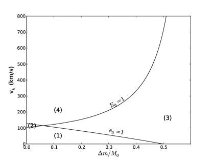
(a) e₀ = 0, E₀ = 0, $\theta_{0}$ = 0^∘, $\Theta_{0}$ = 0^∘, i₀ = 0, $\alpha_{0}$ = 0^∘,
$\mathbf{\hat{v}_{k}}$ = (1,0,0)

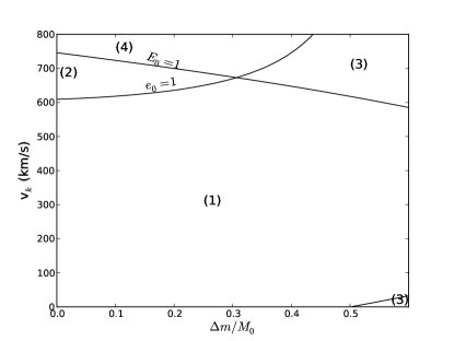
(b) e₀ = 0, E₀ = 0, $\theta_{0}$ = 0^∘, $\Theta_{0}$ = 0^∘, i₀ = 0, $\alpha_{0}$ = 0^∘,
$\mathbf{\hat{v}_{k}}$ = (-1,0,0)

Figure 3: The plots above show the survivability of the hierarchical triple system for varying mass loss $\Delta m$ and kick velocity $v_{k}$. The systems have masses of m_1,0, m₂, m₃ = 3, 2, 1 M_⊙ respectively and inner and outer binary semi-major axes a₀, A₀ = 10, 50 R_⊙ respectively. There are four possible post-SN scenarios: (1) the whole triple survives, (2) the inner binary survives but the third star escapes, (3) the inner binary dissociates and the outer binary survives, or (4) the triple completely dissociates. The areas in the plots are labeled according to their respective post-SN scenario.

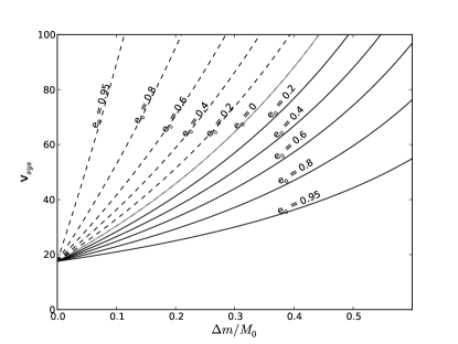
(a)

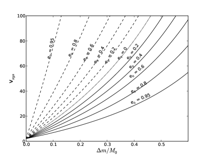
(b)

Figure 4: The post-SN systemic velocity of the triple as a function of mass loss, $\Delta m$, when the SNe occurs at periastron ($\theta_{0}=0$, dashes) and apastron ($\theta_{0}=180$ degrees, solid curves) of the inner binary, for a range of pre-SN inner binary eccentricities. $v_{k}=0$ km/s in the top panel and $\sim 31$ km/s in the bottom panel.

2.4 Hierarchical systems of multiplicity $\mn@boldsymbol{>3}$

There exist two kind of hierarchical multiple star systems with more than three stars:

1. systems that have $n$ stars and hierarchy $n-1$, i.e. multiple star systems with its stars hierarchically ordered in series (hereafter serial systems). Examples of such systems include quadruples with hierarchy 3, but also binaries and triples are serial systems.

2. systems that have $n$ stars and hierarchy $n-2$ or below, i.e. multiples composed of serial systems which are hierarchically ordered in parallel (hereafter parallel systems). An example of such system is a quadruple with hierarchy 2 (i.e. a binary-binary system).

2.4.1 Serial systems

The effect of a SN on a serial system is calculated by applying the effective binary method (see section 2.2) by recursively replacing the inner binary by an effective star at the center of mass of that binary, until the total system is reduced to a single effective binary. When considering a serial system of $n$ stars each with mass, position and velocity given by ($m_{1,0}$,$\mathbf{r_{1}}$,$\mathbf{v_{1,0}}$), ($m_{2}$,$\mathbf{r_{2}}$,$\mathbf{v_{2}}$), … , ($m_{n}$,$\mathbf{r_{n}}$,$\mathbf{v_{n}}$) respectively, in which the primary star undergoes a SN, one starts by reducing the inner binary to an effective star, as was done in section 2.2. The inner binary consists of the primary and secondary star at positions $\mathbf{r_{1}}$ and $\mathbf{r_{2}}$ respectively. This binary is reduced to an effective star of mass $m_{cm,0}=m_{1,0}+m_{2}$ at position $\mathbf{r_{cm,0}}$ given by equation (17) and having velocity $\mathbf{v_{cm,0}}$ given by equation (18). Due to the SN of the primary this effective star experiences a mass loss $\Delta m$, an instantaneous translation $\mathbf{\Delta R}$ given by equation (19), and a random kick velocity $\mathbf{v_{sys}}$ given by equation (2.1). After applying these effects on this effective binary, one can calculate the post-SN orbital parameters and velocities and the systemic velocity $\mathbf{v_{sys}^{(2)}}=\mathbf{V_{sys}}$ of this effective binary, given by equation (31), using the prescription for a SN in a binary. The total system is now reduced to a serial system of $n-1$ objects (real and effective stars).

Subsequently, one reduces the current inner binary - consisting of the effective and tertiary star at positions $\mathbf{r_{cm,0}}$ and $\mathbf{r_{3}}$ respectively - to an effective star of mass $m_{cm,0}^{(2)}=m_{cm,0}+m_{3}$, at position

$$\mathbf{r_{cm,0}^{(2)}}=\frac{m_{cm,0}\mathbf{r_{cm,0}}+m_{3}\mathbf{r_{3}}}{m_{cm,0}+m_{3}}$$ (36)

with a velocity

$$\mathbf{v_{cm,0}^{(2)}}=\frac{m_{cm,0}\mathbf{v_{cm,0}}+m_{3}\mathbf{v_{3}}}{m_{cm,0}+m_{3}}.$$ (37)

Due to the SN of the primary star, this effective star also experiences a mass loss $\Delta m$, an instantaneous translation $\mathbf{\Delta R^{(2)}}$ - this time, the translation vector has non-zero y- and z-components - and a random kick velocity $\mathbf{v_{sys}^{(2)}}$. After applying these effects on this effective binary, one can calculate the post-SN orbital parameters and velocities and the systemic velocity $\mathbf{v_{sys}^{(3)}}$ of this effective binary using the prescription for a SN in a binary. The total system is now reduced to a serial system of $n-2$ objects (real and effective stars).

This procedure is carried on until the entire multiple is reduced to a single effective binary, consisting of the $n$th star at position $\mathbf{r_{n}}$ and a effective star of mass $m_{cm,0}^{(n-2)}=m_{cm,0}^{(n-3)}+m_{n-1}$ at position

$$\mathbf{r_{cm,0}^{(n-2)}}=\frac{m_{cm,0}^{(n-3)}\mathbf{r_{cm,0}^{(n-3)}}+m_{n-1}\mathbf{r_{n-1}}}{m_{cm,0}^{(n-3)}+m_{n-1}}$$ (38)

with a velocity

$$\mathbf{v_{cm,0}^{(n-2)}}=\frac{m_{cm,0}^{(n-3)}\mathbf{v_{cm,0}^{(n-3)}}+m_{n-1}\mathbf{v_{n-1}}}{m_{cm,0}^{(n-3)}+m_{n-1}}.$$ (39)

This effective star also experiences mass loss $\Delta m$, an instantaneous translation $\mathbf{\Delta R^{(n-2)}}$ and a random kick velocity $\mathbf{v_{sys}^{(n-2)}}$. After applying these effects on this (final) effective binary, one can calculate the post-SN orbital parameters and velocities and the systemic velocity $\mathbf{v_{sys}^{(n-1)}}$ for this effective binary (and therefore of the total system) using the binary method.

When it is not the primary star which undergoes a SN, but the $m$th star in the hierarchy, the procedure is carried out by first reducing the inner serial system of $m-1$ stars to an effective star at its center of mass. One can then apply the above explained method, as there is no computational difference in whether the primary or the secondary of a(n effective) binary undergoes the SN.

2.4.2 Parallel systems

The effect of a SN on a parallel system is calculated by reducing each parallel branch (which itself is a serial system) to an effective star until an effective serial configuration is reached; after this, one can use the method explained in the previous section. We consider a parallel system of $i$ parallel branches, each consisting of an arbitrary number $n_{i}$ of stars with mass, position and velocity given by ($m_{1}$,$\mathbf{r_{1}}$,$\mathbf{v_{1}}$), … , ($m_{n_{i}}$,$\mathbf{r_{n_{i}}}$,$\mathbf{v_{n_{i}}}$) respectively, in which the $m$th star - which is part of branch $j$ - undergoes a SN. One starts by reducing all $i-1$ branches $\neq j$ to effective stars. One then calculates the effect of the SN on branch $j$ (i.e. systemic velocity and mass loss) using the method described in section 2.4.1. The total system is now reduced to an effective serial system of $i$ effective stars in which the $j$th effective star undergoes an effective SN with the systemic velocity of branch $j$ as the kick velocity. The effect of this effective SN on the total system, can be calculated by applying the method described in section 2.4.1 to this effective serial system. As an example we will now demonstrate the effect of a SN on a binary-binary system.

2.4.3 An example of the effect of a supernova in binary-binary system

We consider a hierarchical binary-binary system of stars with mass, position and velocity given by ($m_{1,0}$,$\mathbf{r_{1}}$,$\mathbf{v_{1,0}}$), ($m_{2}$,$\mathbf{r_{2}}$,$\mathbf{v_{2}}$), ($m_{3}$,$\mathbf{r_{3}}$,$\mathbf{v_{3}}$) and ($m_{4}$,$\mathbf{r_{4}}$,$\mathbf{v_{4}}$) respectively, in which the primary star undergoes a SN. The binary consisting of the primary and the secondary star (primary binary) has the configuration and the parameters as in section 2.1 and has a center of mass (cm₁, i.e. effective star 1) of mass $m_{cm1,0}=m_{1,0}+m_{2}=M_{0}$ at position given by equation (17) with a velocity $\mathbf{v_{cm1,0}}$ given by equation (18). The secondary binary consists of the tertiary and quaternary star and its center of mass (cm₂, i.e. effective star 2) has a mass $m_{cm2}=m_{3}+m_{4}=M_{2}$, is at position

$$\mathbf{r_{cm2}}=(1-\kappa)\mathbf{r_{3}}+\kappa\mathbf{r_{4}}$$

and has velocity

$$\mathbf{v_{cm2}}=(1-\kappa)\mathbf{v_{3}}+\kappa\mathbf{v_{4}},$$

before the SN, where $\kappa=\frac{m_{4}}{M_{2}}$. The cm₁ and cm₂ constitute an effective binary defined by semi-major axis, $A_{0}$, eccentricity, $E_{0}$, and true anomaly, $\Theta_{0}$. The separation distance is denoted by ${\mathbf{R}}_{0}$. Before the SN the effective binary orbital plane has inclination $i_{0}$ with respect to the primary binary orbital plane and the separation distance of the effective binary projected onto the xy-plane makes an angle $\alpha_{0}$ with the separation distance of the primary binary. We assume an instantaneous SN. In the effective SN the cm₁ experiences a mass loss $\Delta m$, an instantaneous translation $\mathbf{\Delta R}$ along the x-axis given by equation (19) and a random kick velocity $\mathbf{v_{sys}}$ given by equation (2.1). The orbital parameters change as a result of the SN: the primary binary parameters change according to the description in section 2.1 and the effective binary orbital parameters change to semi-major axis $A$, eccentricity $E$ and true anomaly $\Theta$; the secondary binary orbital parameters do not change when SN-shell impact is not taken into account. Before the SN the binary-binary system has a total mass $M_{bb,0}=m_{cm1,0}+m_{cm2}$, we use the cm₁ coordinate system to pin down the primary binary and add to this coordinate system the tertiary and quaternary at a position such that $R_{0}\gg r_{0}$, and we choose a reference frame in which the center of mass of the total binary-binary system (CM_bb) is at rest (the CM_bb reference frame) and in which the cm₁ is at the origin at $t=0$. The separation distance between the cm₁ and the cm₂, $\mathbf{R_{0}}$, is given by equation (20) and the velocity of the cm₁ relative to the cm₂ is

$$\mathbf{V_{0}}=\mathbf{v_{cm1,0}}-\mathbf{v_{cm2}}=(V_{0x},V_{0y},V_{0z})$$ (40)

prior to the SN. The effective kick velocity $\mathbf{v_{sys}}$ makes an angle $\Phi$ with the pre-SN relative velocity $\mathbf{V_{0}}$. After the SN the separation distance between the cm₁ and the cm₂ is $\mathbf{R}$ given by equation (22) and the velocity of the cm₁ relative to the cm₂ is $\mathbf{V}$ given by equation (23), the cm₁ mass $m_{cm1}=m_{cm1,0}-\Delta m=M$ and total binary-binary mass $M_{bb}=m_{cm1}+m_{cm2}=M+M_{2}$. Applying the relations above and equations (1) and (2) to our binary-binary system, we obtain relations for the post-SN semi-major axis $A$ and eccentricity $E$ in terms of both the pre- and post-SN orbital parameters and velocities given by equations (26) and (2.2) respectively with $M_{t,0}$ replaced by $M_{bb,0}$. To compute the systemic velocity due to the SN, we express the pre-SN velocities of the cm₁ and the cm₂ in the CM_bb reference frame. Using the pre-SN mass ratio $\lambda_{0}=\frac{m_{cm2}}{M_{bb,0}}$, the pre-SN velocities are given by

$$\mathbf{v_{cm1,0}} = \lambda_{0}\Bigl{(}V_{0x},V_{0y},V_{0z}\Bigr{)}$$ (41)

$$\mathbf{v_{cm2}} = (\lambda_{0}-1)\Bigl{(}V_{0x},V_{0y},V_{0z}\Bigr{)}.$$ (42)

We calculate the instantaneous velocity of the cm₁ after the SN (due to the assumption of an instantaneous SN, the velocity of the cm₂ after the SN remains unchanged):

$$\mathbf{v_{cm1}}=\lambda_{0}\Bigl{(}V_{0x}+\frac{v_{sys,x}}{\lambda_{0}},V_{0y}+\frac{v_{sys,y}}{\lambda_{0}},V_{0z}+\frac{v_{sys,z}}{\lambda_{0}}\Bigr{)}$$ (43)

With the post-SN mass ratio $\lambda=\frac{m_{cm2}}{M_{bb}}$, the systemic velocity of the effective binary (and therefore of the binary-binary system) is

$$\mathbf{V_{sys}} = (1-\lambda)\mathbf{v_{cm1}}+\lambda\mathbf{v_{cm2}}$$ (44)

$$= (1-\lambda)\Bigl{(}\frac{\lambda_{0}-\lambda}{1-\lambda}V_{0x}+(\mu_{0}-\mu)v_{0x}+(1-\mu)v_{kx},$$

$$\frac{\lambda_{0}-\lambda}{1-\lambda}V_{0y}+(\mu_{0}-\mu)v_{0y}+(1-\mu)v_{ky},$$

$$\frac{\lambda_{0}-\lambda}{1-\lambda}V_{0z}+(1-\mu)v_{kz}\Big{)}.$$

Note that because the branch harboring the SN-progenitor (SN branch) is a binary, this calculation the SN-effect on the binary-binary system is almost identical to calculation of the SN-effect on a hierarchical triple. The computations become more interesting for systems with a SN branch of higher multiplicity.

3 Application: Formation of J1903+0327

PSR J1903+0327 was observed by Champion et al. (2008) who determined it to be a millisecond pulsar (MSP). This MSP is observed to have a 1 $M_{\odot}$ main sequence companion with a highly eccentric and distant orbit ($e$ $\simeq$ 0.44, orbital period $\simeq$ 95.2 days). These properties are atypical for MSPs because MSPs are expected to be spun-up via mass transfer (Bhattacharya & van den Heuvel 1991), which in turn widens and circularizes the orbit, while its companion evolves through a giant phase. Phinney (1992), for example, suggest an eccentricity $e<10^{-3}$ is typical for MSP binaries. The exception to this has been MSPs in globular clusters which have interactions with other objects that may perturb the orbit of the binary. However, Freire et al. (2011) find it to be unlikely that this MSP system has its origin in an exchange interaction in such a dense stellar environment.

It has been suggested that J1903+0327 maybe the result of a hierarchical triple (Champion et al. 2008, Portegies Zwart et al. 2011 and Bejger et al. 2011) where the inner companion has been lost after spinning-up the MSP, leaving only the MSP and the former tertiary to be observed. Should J1903+0327 be the result of such a system the methods in the previous sections provide a strong beginning to investigate how such a system might evolve.

3.1 Initial conditions

We generate sets of $10^{5}$ initial conditions, as described below, with each set constituting a stable triple system, and then simulated the effect of an instantaneous SN occurring at the primary star. The model we follow (many of our initial conditions are drawn from Portegies Zwart et al. (2011)) consist of a primary, secondary and tertiary star with zero age masses of 10 $M_{\odot}$, 1 $M_{\odot}$ and 0.9 $M_{\odot}$ respectively. The initial conditions are generated by selecting the semi-major axis, $A_{0}$, eccentricity, $E_{0}$, and the orbital inclination, $i$, for the tertiary. $A_{0}$ takes values on the range [200, 10 000]$R_{\odot}$ from a flat distribution, $E_{0}$ is chosen on the range [0, 1) from a distribution that is flat in log space, and $i_{0}$ is chosen on the range [0, $\pi$] with a sinusoidal distribution. Combining these values with the zero age masses of the stars as well as a pre-set value for the initial semi-major axis of the inner binary, $a_{0}=200R_{\odot}$ we then test for stability of the system using:

$$\frac{A_{0}(1-E_{0})}{a_{0}} > 3\Bigl{(}1+\frac{m_{3}}{M_{0}}\Bigr{)}^{1/3}\Bigl{(}\frac{7}{4}+\frac{1}{2}\cos i_{0}-\cos^{2}i_{0}\Bigr{)}^{1/3}$$ (45)

$$\times (1-E_{0})^{-1/6}$$

(Zhuchkov et al. 2010). If the system is stable with this set of parameters, we choose the remaining parameters, namely the angle $\alpha_{0}$ described in the previous sections, the direction and magnitude of the kick. Because we have assured that the system is dynamically stable before starting our simulations our assumption of a hierarchical system is guaranteed. We observe that due to the SN kick, systems with very high inclination are preferentially removed or their inclination is reduced thus as a result we do not include the effects of Kozai iterations.

3.2 Simulations

The inner binary undergoes a common envelope (CE) phase, circularizing the orbit, reducing the inner semi-major axis to a value between 5 $R_{\odot}$ and 60 $R_{\odot}$, and reducing the mass of the primary to 2.7 $M_{\odot}$. The effect of these changes on the stability of the system can immediately be seen in equation (45). Then, due to the SN, the primary undergoes a mass loss of 1.3 $M_{\odot}$ and receives a corresponding kick. The velocity of the kick is fixed between 5 and 160 km/s for each set of simulations and the kick direction is randomly chosen such that for all simulations the direction is isotropic. We then analyze the survivability and stability of each system. A system survives the SN and resulting kick if it remains bound, and it is determined to be stable if, while remaining bound, the system also satisfies the stability criterion in equation (45).

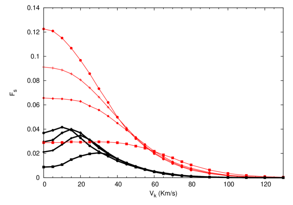
Figure 5: The fraction of surviving and stable system (thin red and thick black (colors online only) lines respectively) as a function of the kick velocity. The lines in each set correspond to different semi-major axis, 50, 30, 20, and 10 $R_{\odot}$ (circle, cross, diamond, and square respectively). All curves are normalized to the total number of surviving systems with a semi-major axis of 50 $R_{\odot}$.

We ran Monte Carlo simulations for four different inner binary semi-major axes (10, 20, 30, and 50 $R_{\odot}$). For each semi-major axis value we run 25 simulations (each of the 25 simulations consists of $10^{5}$ sets of initial conditions) each with a constraint kick velocity (between 0 and 130 km/s). In Figure 5 we plot the kick velocity versus the fraction of surviving and stable systems. For each pair of curves the thin red upper curve corresponds to the survivability fraction and the thick black lower curve to the fraction that survives and remains stable. Curves with same kick velocity have the same point-symbols. Each point represents the fraction of surviving or stable systems normalized to the total number of surviving systems with a semi-major axis of 50$R_{\odot}$. Increasing the semi-major axis from 10 to 30 $R_{\odot}$ strongly increases the overall probability of a system to survive and remain stable. However, with a kick velocity of 45 km/s and higher the probability of a system remaining stable is nearly the same when the semi-major axis is $\geq$ 20$R_{\odot}$. Figure 5 shows the effect of the Blaauw $\&$ Boersma recoil (Blaauw 1961 $\&$ Boersma (1961)) on the system when the SN kick is small; as the SN kick velocity approaches the Blaauw $\&$ Boersma recoil velocity the stability increases due to the kick and recoil off-setting one another, in part or in full. As the SN kick velocity increases it begins to overwhelm the Blaauw $\&$ Boersma effect.

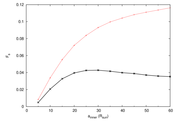
Figure 6: The fraction of surviving and stable systems (upper and lower lines respectively) with respect to the inner semi-major axis. A constant kick velocity of 20 km/s is used.

In Figure 6 we show the effect the inner semi-major axis has on survivability and stability (the upper and lower lines respectively) using a constant kick velocity of 20 km/s. Again each data point represents the fraction of systems that survive or survive and in addition remains stable out of a set of $10^{5}$ initial conditions. Here we see the significant role of the inner semi-major axis on the survivability of the system. If we note for a particular kick velocity which value of $a_{0}$ the stability fraction begins to level, we can see it corresponds to the merging of the stability curves in Figure 5. For the case of a 20 km/s SN kick velocity, as in Figure 6, we see that any value of $a_{0}$ greater than about 30 $R_{\odot}$ will have similar stability fractions while systems with lower values of $a_{0}$ should have a lower stability fraction as we see in Figure 5.

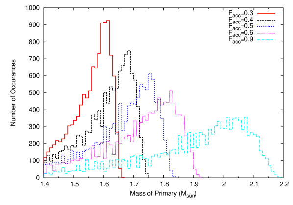
Figure 7: The number of occurrences for which the system becomes unstable due to mass transfer at a given mass of the primary. The curves corresponds to $F_{acc}$ values of 0.3, 0.4, 0.5, 0.6, and 0.9 as shown in the key. The peak value and FWHM for each curve in this figure, as well as similar curves for other values of $F_{acc}$, are plotted in Figure 8.

Next, we chose all of the systems that remain stable after the SN and subject them to a mass transfer phase. Here we iteratively remove one one-hundredth of the mass of the secondary and transfer a fraction of it to the primary, which after the SN would have formed a neutron star (NS). Following the work of Pols & Marinus (1994) we find:

$$a_{f}=a_{i}\Bigl{[}\Bigl{(}\frac{m_{1,f}}{m_{1_{i}}}\Bigr{)}^{(1/(1-\chi))}\frac{m_{2,f}}{m_{2_{i}}}\Bigr{]}^{-2}\times\Bigl{(}\frac{M_{i}}{M_{f}}\Bigr{)}$$ (46)

where $a_{f}$ is the new semi-major axis, $a_{i}$ is the semi-major axis before the mass transfer, $m_{1,i}$ and $m_{2,i}$ are the masses of the primary and secondary before the mass transfer and $m_{1,f}$ and $m_{2,f}$ are the masses of the primary and secondary after the mass transfer, $M_{i}$ and $M_{f}$ are the total masses of the binary before and after the mass transfer, and finally $\chi$ is the ratio of the change in mass of the system to the change in mass of the donor (i.e. the secondary). If we define the fraction of mass accreted, $F_{acc}$, as the fraction of mass lost from the secondary which is accreted onto the primary we find that the $1/(1-\chi)$ term simply becomes $1/F_{acc}$.

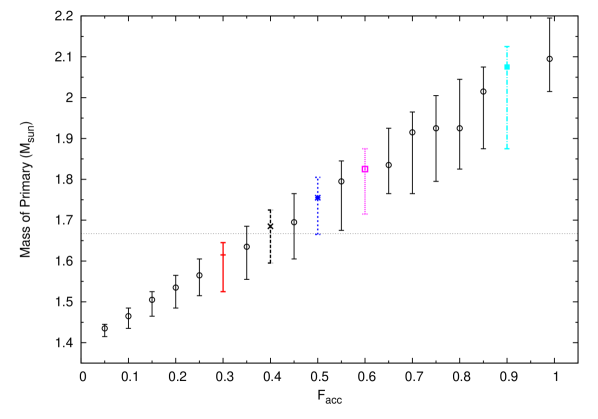
Figure 8: The final mass of primaries with respect to the fraction of accreted mass. The dashed horizontal line is placed at the observed mass of J1903+0327. The points represent the peak value of curves which plot the number of times a system becomes unstable while at a given mass of the primary (like those in Figure 7); the upper and lower bars represent the FWHM of the curves. The values that are colored (online) and that have different line types correspond to the curves in Figure 7 (e.g. the blue, dot-dash line at $F_{acc}$=0.9 is obtained from the right most peaked curve in Figure 7, which is also a blue, dot-dash line).

After each iterative mass transfer, and the resulting change in the semi-major axis, we test the triple for stability using equation (45). When the system becomes dynamically unstable we stop simulating as the assumption of a hierarchical system has broken down. We record the mass of the primary when the system becomes dynamically unstable and plot the mass in Figure 7 versus the number of times systems becomes unstable at that mass. For this plot we used $F_{acc}$ values of 0.3, 0.4, 0.5, 0.6 and 0.9, which correspond to the lines which peak from the left to right respectively, and a constant kick velocity. We see that the peak value for each $F_{acc}$ shifts to a larger primary mass as $F_{acc}$ increases. This relation is expected since as $F_{acc}$ becomes larger more of the mass lost from the secondary is accreted onto the primary. So for the case of $F_{acc}=0.3$ only $30\%$ of the mass lost from the secondary could ever accrete onto the primary thereby reducing the maximum possible mass of the primary. If we assumed that all of the mass of the secondary is lost (an unphysical case since the mass transfer would end before this could happen, but this provides an extreme upper limit) then while the secondary would have lost 1$M_{\odot}$ the primary would have only accreted 0.3$M_{\odot}$ resulting in a maximum primary mass of 1.7 $M_{\odot}$. If we were to assume that mass transfer would stop when the secondary decreased to a mass of 0.3$M_{\odot}$ then the secondary would have lost 0.7$M_{\odot}$ and only 0.21$M_{\odot}$ (or 30% of 0.7$M_{\odot}$) would have been accreted by the primary resulting in a mass of 1.61$M_{\odot}$. We have examined 21 curves like those in Figure 7, we measured and plotted their peak value and the full-width-half-maximum (FWHM) in Figure 8. The error bars denote the FWHM of the curves, the plotted point is the peak value for each curve, and the mass of J1903+0327 is shown as a dashed line. Examination of Figure 8 shows that given the observed mass and the assumptions we used in preparing the simulated systems, J1903+0327’s progenitor system would have most likely had an $F_{acc}$ value between between 0.35 and 0.5, with the peak value of 0.4 most closly maching the observed mass.

It should be noted however, not all of the barionic mass transfered results in an equivalent increase in gravitational mass of the primary since $M_{accrete}$ = $\Delta M_{grav}+\Delta E_{binding}/c^{2}$ (Bagchi 2011), where $M_{accrete}$ is the mass accreted from the secondary, $\Delta M_{grav}$ is the change in gravitational mass of the primary, and $\Delta E_{binding}$ is the binding energy of the system. We find that for the masses being transferred in our simulations the effect of using $M_{accrete}=\Delta M_{grav}$ is less than the uncertainty in the final results.

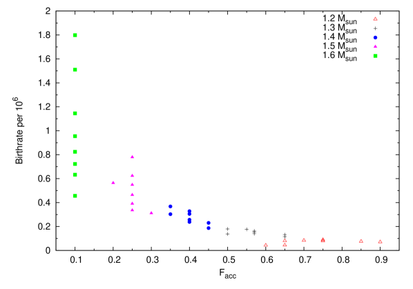
Figure 9: The number of systems per millon simulations with a final primary mass of 1.667 $M_{\odot}$ (the observed mass of J1903+0327) as a function of the fraction of accreted mass, for different initial primary masses (shown in the key).

Finally, we preform the same analysis that produced Figure 7 but use an initial primary mass of 1.2, 1.3, 1.4 (as used in all of the previous simulations), 1.5, and 1.6 $M_{\odot}$. These simulations were preformed for eight inner semi-major axes (10, 20, 30, 40, 50, 60, 70, and 100 $R_{\odot}$) at the start of mass transfer. The $F_{acc}$ value with the peak number of occurrences closest to the observed mass of J1903+0327 (1.667 $M_{\odot}$) was recorded, as was the number of occurrences at that peak; these values were plotted in Figure 9. Upon examining Figure 9 we find that as the initial mass of the primary increases the most likely $F_{acc}$ value and its domain decrease. To understand these results we recall that as the initial mass of the primary increases the amount of mass needed to reach the observed mass of J1903+0327 is decreased. So, for example, if the initial mass of the progenitor of J1903+0327’s primary (before it began to accrete material from the secondary) was 1.6 $M_{\odot}$ it would only need to accrete 0.067 $M_{\odot}$ before the system reached the observed mass. A very small $F_{acc}$ value can result in the transfer of such a small amount of material allowing the $F_{acc}$ to stay low; with a lager $F_{acc}$ value the system will often reach a final primary mass greater than 1.667 $M_{\odot}$ thus limiting the domain. Whereas if the initial primary mass was 1.2 $M_{\odot}$, an $F_{acc}$ value of 0.1 would never allow for enough mass to be transfered, but there are a large range of $F_{acc}$ values that can allow for that amount of mass transfer that would not quickly overshoot the observed mass. This assumes, as we have in all of the simulations, that the mass transfer is stable as long as the triple is dynamically stable. We find that for an initial primary mass of 1.4 $M_{\odot}$, the value used in all previous simulations, the peak $F_{acc}$ value is not sensitive to the semi-major axis at the beginning of the mass transfer; the $F_{acc}$ value ranges between 0.35 and 0.45 which lies within our expected range of 0.35 to 0.5 found above from Figure 8.

4 Conclusion

We have examined the effect of an asymmetric supernova (SN) on a hierarchical multiple star system and considered how it can be modeled by applying the effective binary method. This is done by recursively replacing the inner binary by an effective star at the center of mass of that binary. The effective star experiences an effective SN with the effects of sudden mass loss, an instantaneous translation and an effective kick velocity, i.e. the systemic velocity of the inner binary. We have coded the equations in this paper in a small python script, which is publicly available

We point out that the effective SN is different from a physical SN in that for a physical SN themass is lost from the position of the physical star, whereas for an effective SN the mass is lost from the effective star. The off-center mass loss in an effective SN becomes important only if the shell impact on the companion(s) is considered, and otherwise causes no difference between a real and effective SN calculation. Furthermore, we calculated the runaway velocities for dissociating binaries and effective binaries. We subsequently demonstrated how calculating the effect of a SN on a multiple can be generalized to multiples in which a star other than the primary is undergoing the SN.

We used this method to examine the case for J1903+0327 forming from a hierarchical triple. We assume initial masses of 10, 1.0, and 0.9 $M_{\odot}$ for the primary, secondary, and tertiary respectively, as well as an inner semi-major axis of 200 $R_{\odot}$. We find that if J1903+0367 was to form through such a mechanism it would be most likely to have a very low SN kick velocity so that it would remain stable after the SN, and a large inner semi-major axis after the CE phase to increase the likelihood that the triple would become unstable once the NS/MSP reached a mass of 1.667 $M_{\odot}$ (Freire et al. 2011). We also find that, given our assumptions, the transfer efficiency, $F_{acc}$, for J1903+0327 would have likely been between 0.35 and 0.5.

5 Acknowledgements

We thank Elena Maria Rossi for her useful suggestions. We would also like to thank the referee for his helpful comments which have greatly improved this paper. This work was supported by the Netherlands Research School for Astronomy (NOVA) and the Netherlands Research Council NWO [grants VICI (639.073.803) and AMUSE (614.061.608)].

References

- Bagchi (2011) Bagchi M., 2011, MNRAS , 413, L47
- Bejger et al. (2011) Bejger M., Fortin M., Haensel P., Zdunik J. L., 2011, A&A , 536, A87
- Bhattacharya & van den Heuvel (1991) Bhattacharya D., van den Heuvel E. P. J., 1991, PhysRep , 203, 1
- Blaauw (1961) Blaauw A., 1961, Bul. Astron. Inst. Neth. , 15, 265
- Boersma (1961) Boersma J., 1961, Bul. Astron. Inst. Neth. , 15, 291
- Champion et al. (2008) Champion D. J., Ransom S. M., Lazarus P., Camilo F., Bassa C., Kaspi V. M., Nice D. J., Freire P. C. C., Stairs I. H., van Leeuwen J., Stappers B. W., Cordes J. M., Hessels J. W. T., Lorimer D. R., Arzoumanian Z., Backer D. C., Bhat N. D. R., Chatterjee S., Cognard I., Deneva J. S., Faucher-Giguère C.-A., Gaensler B. M., Han J., Jenet F. A., Kasian L., Kondratiev V. I., Kramer M., Lazio J., McLaughlin M. A., Venkataraman A., Vlemmings W., 2008, Science, 320, 1309
- Freire et al. (2011) Freire P. C. C., Bassa C. G., Wex N., Stairs I. H., Champion D. J., Ransom S. M., Lazarus P., Kaspi V. M., Hessels J. W. T., Kramer M., Cordes J. M., Verbiest J. P. W., Podsiadlowski P., Nice D. J., Deneva J. S., Lorimer D. R., Stappers B. W., McLaughlin M. A., Camilo F., 2011, MNRAS , 412, 2763
- Gunn & Ostriker (1970) Gunn J. E., Ostriker J. P., 1970, ApJ , 160, 979
- Hills (1983) Hills J. G., 1983, ApJ , 267, 322
- Kalogera (1996) Kalogera V., 1996, ApJ , 471, 352
- Phinney (1992) Phinney E. S., 1992, Royal Society of London Philosophical Transactions Series A, 341, 39
- Podsiadlowski et al. (2004) Podsiadlowski P., Langer N., Poelarends A. J. T., Rappaport S., Heger A., Pfahl E., 2004, ApJ , 612, 1044
- Pols & Marinus (1994) Pols O. R., Marinus M., 1994, A&A , 288, 475
- Portegies Zwart et al. (2011) Portegies Zwart S., van den Heuvel E. P. J., van Leeuwen J., Nelemans G., 2011, ApJ , 734, 55
- Shklovskii (1970) Shklovskii I. S., 1970, SvA , 13, 562
- Tauris & Takens (1998) Tauris T. M., Takens R. J., 1998, A&A , 330, 1047
- Tokovinin (1997) Tokovinin A. A., 1997, A&AS , 124, 75
- van den Heuvel & van Paradijs (1997) van den Heuvel E. P. J., van Paradijs J., 1997, ApJ , 483, 399
- Wheeler et al. (1975) Wheeler J. C., Lecar M., McKee C. F., 1975, ApJ , 200, 145
- Zhuchkov et al. (2010) Zhuchkov R. Y., Kiyaeva O. V., Orlov V. V., 2010, Astronomy Reports, 54, 38