Cosmological Constraints from a Combination of Galaxy Clustering & Lensing – II. Fisher Matrix Analysis

Abstract

We quantify the accuracy with which the cosmological parameters characterizing the energy density of matter ($\Omega_{\rm m}$), the amplitude of the power spectrum of matter fluctuations ($\sigma_{8}$), the energy density of neutrinos ($\Omega_{\nu}$) and the dark energy equation of state ($w_{0}$) can be constrained using data from large galaxy redshift surveys. We advocate a joint analysis of the abundance of galaxies, galaxy clustering, and the galaxy-galaxy weak lensing signal in order to simultaneously constrain the halo occupation statistics (i.e., galaxy bias) and the cosmological parameters of interest. We parameterize the halo occupation distribution of galaxies in terms of the conditional luminosity function and use the analytical framework of the halo model described in our companion paper (van den Bosch et al. 2012), to predict the relevant observables. By performing a Fisher matrix analysis, we show that a joint analysis of these observables, even with the precision with which they are currently measured from the Sloan Digital Sky Survey, can be used to obtain tight constraints on the cosmological parameters, fully marginalized over uncertainties in galaxy bias. We demonstrate that the cosmological constraints from such an analysis are nearly uncorrelated with the halo occupation distribution constraints, thus, minimizing the systematic impact of any imperfections in modeling the halo occupation statistics on the cosmological constraints. In fact, we demonstrate that the constraints from such an analysis are both complementary to and competitive with existing constraints on these parameters from a number of other techniques, such as cluster abundances, cosmic shear and/or baryon acoustic oscillations, thus paving the way to test the concordance cosmological model.

1 Introduction

Of the various cosmological models in the literature, the $\Lambda$CDM model has withstood a large variety of observational tests which have grown more and more stringent over time. According to this model, at present times, dark energy and dark matter form the dominant component of the energy density budget of the Universe. Ordinary matter forms a sub-dominant component and is primarily present in the form of gas in the intergalactic medium and around galaxies. Obtaining precise constraints on the energy densities of the various components of the Universe (quantified by the energy density parameters for matter [$\Omega_{\rm m}$], dark energy [$\Omega_{\Lambda}$], baryonic matter [$\Omega_{\rm b}$] and neutrinos [$\Omega_{\nu}$]), is of great importance, in order to understand the expansion history and future fate of the Universe.

Any successful cosmological model also requires to explain the formation of structure in the Universe. The $\Lambda$CDM model assumes the presence of nearly scale invariant, tiny initial fluctuations in the matter density, presumably generated during inflation. Structure grows hierarchically in this model with small scales collapsing first followed by larger and larger scales as the Universe grows old. The precise description of the inhomogeneous Universe requires the knowledge of the index of the power spectrum of initial fluctuations, $n_{\rm s}$ and its amplitude (quantified in terms of the parameter $\sigma_{8}$).

Observations of the fluctuations in the cosmic microwave background on both large (e.g., Spergel et al., 2007; Komatsu et al., 2011) and small scales (e.g., Lueker et al., 2010; Dunkley et al., 2011), of the dimming of distant supernovae as a function of their redshift (e.g., Riess et al., 1998; Perlmutter et al., 1999; Kowalski et al., 2008; Kessler et al., 2009; Guy et al., 2010), of the large scale structure traced by galaxies (e.g., Tegmark et al., 2004; Swanson et al., 2010), of the abundance of massive clusters and its evolution (e.g., Vikhlinin et al., 2009; Mantz et al., 2010; Rozo et al., 2010; Benson et al., 2011; Sehgal et al., 2011), of the angular extent of the baryonic acoustic oscillation scale as a function of redshift (e.g., Eisenstein et al., 2005; Percival et al., 2007, 2010; Blake et al., 2011; Anderson et al., 2012), and of the weak distortion of galaxies due to intervening structure (e.g., Massey et al., 2007; Schrabback et al., 2010; Lin et al., 2011; Huff et al., 2011) have all contributed to enable precise constraints on the parameters that describe the $\Lambda$CDM model. It is remarkable that a single model with a small number of parameters is able to self consistently explain all these observations.

Large spectroscopic galaxy redshift surveys such as the 2-degree field galaxy redshift survey (Colless et al., 2001) and the Sloan digital sky survey (hereafter SDSS, York et al., 2000; Abazajian et al., 2009) have played an important role of mapping out the three-dimensional structure of galaxies in the Universe in exquisite detail. This has allowed precise measurements of the abundance of galaxies and their clustering on non-linear scales as a function of galaxy properties such as luminosity (Wang et al., 2008; Zehavi et al., 2011; Blanton et al., 2003b; Norberg et al., 2001), stellar mass (Li et al., 2007; Baldry et al., 2008; Cole et al., 2001), or colour (Norberg et al., 2002; Wang et al., 2008; Swanson et al., 2008; Zehavi et al., 2011). The halo model has traditionally been used to obtain the halo occupation distribution of galaxies given a cosmological model based on these observations (e.g., Jing et al., 1998; Berlind & Weinberg, 2002; Yang et al., 2003; Zheng et al., 2005; van den Bosch et al., 2007; Zheng et al., 2007; Tinker et al., 2005; Zehavi et al., 2011; Coupon et al., 2011; Leauthaud et al., 2012). A few studies however have also turned the question around to judge if these observations can be used to constrain the cosmological parameters themselves (van den Bosch et al., 2003, 2007; Tinker et al., 2005; Yoo et al., 2006; Cacciato et al., 2009; Tinker et al., 2012).

Galaxies reside in dark matter haloes. The cosmological parameters determine the abundance and clustering of dark matter haloes of a given mass. Therefore, the observations of the abundance and clustering of galaxies is sensitive to various cosmological parameters and can be used to constrain these parameters. However, this requires the knowledge of an accurate mapping between galaxies and their dark matter haloes. In Cacciato et al. (2009), we highlighted this problem, by demonstrating that two different cosmological models, (differing primarily in $\Omega_{\rm m}$ and $\sigma_{8}$) were able to simultaneously fit the galaxy abundance and the galaxy-galaxy clustering data by adjusting the halo occupation distribution of galaxies. However, we also showed that these models make vastly different predictions for the amount of baryons that should occupy dark matter haloes, quantified by the mass-to-light ratio (see also van den Bosch et al., 2003, 2007; Tinker et al., 2005; Yoo et al., 2006). Galaxy-galaxy lensing, which measures the projected galaxy-matter correlation function is an excellent probe of the mass-to-light ratios. Therefore, it was suggested that a joint analysis of the abundance, clustering and lensing of galaxies can be used to obtain constraints on cosmological parameters such as $\Omega_{\rm m}$ and $\sigma_{8}$.

This paper is the second in a series of three papers in which we develop this idea further. In van den Bosch et al. (2012, hereafter Paper I) we describe our model for the halo occupation distribution of galaxies and present an analytical framework for the computation of the abundance of galaxies, their clustering and the galaxy-matter cross correlation. We make extensive use of mock catalogs to validate our analytical prescription and show that our analytical model is accurate to better than 10 (in most cases 5) percent in reproducing the 3-dimensional galaxy-galaxy correlation and galaxy-matter correlation. These correlations can then be projected to predict the galaxy clustering and the galaxy-galaxy lensing signal measured from SDSS data. In this paper, we perform a Fisher matrix analysis to forecast the accuracy with which various cosmological parameters can be constrained with current data. The analysis allows us to understand the strength of each of our data-sets as well as the various degeneracies between our model parameters. In Cacciato et al. (2012, hereafter Paper III), we apply our method to data from the SDSS, simultaneously constraining galaxy bias and cosmology.

This paper is organized as follows. In section 2, we briefly describe the data and our analytical model. In section 3, we describe the Fisher information matrix corresponding to the observables. In section 4, we present the constraints on our model parameters that are statistically achievable given the accuracy of the data. Finally, we summarize our results in Section 5 and provide a future outlook.

2 Data and the analytic model

Our analysis is based on galaxy observations carried out as part of the spectroscopic component of the SDSS. In particular, we focus on the accurate measurements of the galaxy luminosity function (Blanton et al., 2003a), the clustering of galaxies in six different luminosity bins (Zehavi et al., 2011) on scales ranging from $0.17\>h^{-1}{\rm{Mpc}}$ to $42.3\>h^{-1}{\rm{Mpc}}$, and the galaxy-galaxy lensing signal around galaxies in different luminosity bins (Mandelbaum et al., 2006) on scales ranging from $0.045\>h^{-1}{\rm{Mpc}}$ to $1.81\>h^{-1}{\rm{Mpc}}$. Our aim is to perform a Fisher matrix analysis to understand the extent to which these datasets constrain the cosmological parameters that we are interested in and the various degeneracies that enter our analysis. For this purpose, we choose a set of fiducial parameters that describe the cosmology (see Table 1) and the halo occupation distribution of the galaxies (see Table 2). We use the analytical model (see Sections 2.1-2.4) to predict galaxy abundances, galaxy clustering (in projection), and the galaxy-galaxy lensing signal (always using the same luminosity bins and radii as in the SDSS data). We assume that these observables are measured with a percentage accuracy that is listed in Table 3 and chosen such that the measurement quality is fairly similar to that of actual SDSS measurements.

We perform three different analyses, that correspond to the $\Lambda$CDM model and its variants. For the first analysis, we assume a flat standard $\Lambda$CDM cosmology with a negligible amount of energy density in neutrinos. We primarily focus on the matter density parameter, $\Omega_{\rm m}$ and the parameter that characterizes the amplitude of matter fluctuations, $\sigma_{8}$. We use priors on the secondary cosmological parameters, the baryon energy density parameter ($\Omega_{\rm b}$), the Hubble parameter ($h=H_{0}/100\>{\rm km}\,{\rm s}^{-1}\,{\rm Mpc}^{-1}$) and the power law index of the initial power spectrum of density fluctuations ($n_{\rm s}$) from the analysis of the 7 year data from WMAP (Komatsu et al., 2011). This is the fiducial model and set of priors which will also be used in Paper III. For the second analysis, we allow for the presence of a non-zero neutrino mass which gives rise to a non-zero neutrino density parameter, $\Omega_{\nu}$. We assume uninformative prior information about $\Omega_{\nu}$ (except that it is positive-definite) and also continue to use uninformative priors on $\Omega_{\rm m}$ or $\sigma_{8}$. For the third analysis, we restore our assumption of a negligible amount of neutrino energy density, but this time add the parameter $w_{0}$ that describes the dark energy equation of state (EoS), such that

$$w_{0}=P_{\Lambda}/(c^{2}\,\rho_{\Lambda})\,.$$ (1)

Here $P_{\Lambda}$ describes the pressure exerted by dark energy and $\rho_{\Lambda}$ denotes its energy density.

Table 1: Cosmological model parameters

Cosmological	Model A	Model B	Model C
parameters
$\Omega_{\rm m}$	0.266	0.266	0.266
$\Omega_{\rm K}$	0.0†	0.0†	0.0†
$\Omega_{\rm b}h^{2}$	0.02258∗	0.02258∗	0.02258∗
$\Omega{\nu}$	0.0†	0.004	0.0†
$\sigma_{8}$	0.801	0.801	0.801
$n_{\rm s}$	0.963∗	0.963∗	0.963∗
$h$	0.71∗	0.71∗	0.71∗
$w_{0}$	-1.0†	-1.0†	-1.0

Cosmological model parameters used to generate artificial datasets. We use a prior given by the covariance matrix of the WMAP chain for the parameters marked with an asterisk. The parameters marked with a dagger are kept fixed when analysing the model for the fiducial case. We discuss variations on some of the assumed priors in the text.

Table 2: CLF and nuisance model parameters

Central CLF	x$L_{0}$	x$M_{1}$	$\gamma_{1}$	$\gamma_{2}$	$\sigma_{\rm c}$
	9.93	11.19	3.5	0.25	0.156
Satellite CLF	$b_{0}$	$b_{1}$	$b_{2}$	$\alpha_{\rm s}$
	-1.08	1.46	-0.20	-1.15
Nuisance	${\eta}$	$\psi$
	1.0	0.903

Model parameters used to describe the central and satellite CLFs. Bottom row shows the values of the nuisance parameters in our model that we assumed for the Fisher analysis.

Table 3: Luminosity bins of the SDSS clustering data

${}^{0.1}M_{\rm r}-5\log h$	$\langle z\rangle$	$w_{\rm p}$ accuracy	$\Delta\Sigma$ accuracy
(1)	(2)	(3)	(4)
$(-19.0,-18.0]$	0.047	30%	50%
$(-20.0,-19.0]$	0.071	30%	20%
$(-21.0,-20.0]$	0.10	5%	15%
$(-21.5,-21.0]$	0.14	5%	15%
$(-22.0,-21.5]$	0.17	5%	15%
$(-22.5,-22.0]$	0.20	40%	15%

Luminosity bins. Column (1) indicates the magnitude range of each luminosity bin (all magnitudes are K$+$E corrected to $z=0.1$). Column (2) indicates the mean redshift of the lens galaxies in each luminosity bin. Column (3) indicates the accuracy of the galaxy clustering data and column (4) indicates the accuracy of the galaxy-galaxy lensing data. The luminosity function data have a fractional accuracy of $\sim 4\%$, and this accuracy degrades to about $\sim 10-15\%$ at the bright and the faint ends respectively.

2.1 The Conditional Luminosity Function

We use the conditional luminosity function (CLF) model described in Paper I to specify our halo occupation distribution. Readers familiar with our model from Paper I may want to proceed directly to Section 3.

The CLF, $\Phi(L|M)\,{\rm d}L$, is defined to be the average number of galaxies with a luminosity $L\pm{\rm d}L/2$ that reside in a halo of mass $M$ (Yang et al., 2003). The CLF consists of a contribution from central galaxies, $\Phi_{\rm c}(L|M)$, and from satellite galaxies, $\Phi_{\rm s}(L|M)$. The distribution $\Phi_{\rm c}(L|M)$ is described by a lognormal distribution with a scatter, $\sigma_{\rm c}$, that is independent of halo mass, consistent with the findings from studies of satellite kinematics (More et al., 2009a, b, 2011) and galaxy group catalogues (Yang et al., 2009). The dependence of the logarithmic mean luminosity, $\log\tilde{L}_{\rm c}$, on halo mass is given by

$$\log\tilde{L}_{\rm c}(M)=\log\left[L_{0}\frac{(M/M_{1})^{\gamma_{1}}}{\left[1+(M/M_{1})\right]^{\gamma_{1}-\gamma_{2}}}\right]\,.$$ (2)

Four parameters are required to describe this dependence; two normalization parameters, $L_{0}$ and $M_{1}$ and two parameters $\gamma_{1}$ and $\gamma_{2}$ that describe the slope of the $\tilde{L}_{\rm c}(M)$ relation at the low mass end and the high mass end, respectively.

The satellite CLF, $\Phi_{\rm s}(L|M)$ is assumed to be a Schechter-like function,

$$\Phi_{\rm s}(L|M){\rm d}L=\Phi_{\rm s}^{*}\left(\frac{L}{L_{*}}\right)^{\alpha_{\rm s}}\,\exp\left[-\left(\frac{L}{L_{*}}\right)^{2}\right]\,\frac{{\rm d}L}{L_{*}}.$$ (3)

Here $L_{*}(M)$ determines the knee of the satellite CLF and is assumed to be a factor $f_{\rm s}$ times fainter than $\tilde{L}_{\rm c}(M)$. Motivated by results from the SDSS group catalog of Yang et al. (2008), we set $f_{\rm s}=0.562$ and assume that the faint-end slope of the satellite CLF is independent of halo mass. The logarithm of the normalization, $\Phi_{\rm s}^{*}$ is assumed to have a quadratic dependence on $\log M$ described by three free parameters, $b_{0}$, $b_{1}$ and $b_{2}$;

$$\log\Phi_{\rm s}^{*}=b_{0}+b_{1}\,(\log M-12)+b_{2}\,(\log M-12)^{2}\,.$$ (4)

Note that this functional form does not have a physical motivation; it merely provides an adequate description of the results obtained by Yang et al. (2008) from the SDSS galaxy group catalog. In addition to specifying the luminosity dependence of the halo occupation distribution, we also need to specify the spatial distribution of galaxies in dark matter haloes. Throughout, we assume that central galaxies reside at the center of their haloes and that the satellite galaxies follow the matter distribution without any spatial bias. The matter density distribution is given by the NFW profile (Navarro et al., 1997) with a concentration that depends upon mass according to the calibration presented in Macciò et al. (2007). As described in Paper I, we allow a $10$ percent uncertainty in the calibration of the normalization of the concentration-mass relation to account for our neglect of the baryonic effects on the matter distribution of halos and the scatter in the concentration-mass relation. We express this uncertainty as a multiplicative parameter ${\eta}$ to the fiducial concentration-mass relation and marginalize over this nuisance parameter. We use the parameters listed in Table 2 for all the three cosmological models.

In all our models the abundance and clustering of dark matter haloes is set by the cosmological parameters, while the halo occupation distribution, as parameterized by the CLF, describes how this abundance and clustering of haloes translates into the abundance and clustering of galaxies as well as their cross correlation with matter. In what follows, we briefly describe the expressions that can be used to compute the model predictions for the data described above.

2.2 Galaxy Luminosity Function

Given the cosmological parameters and the parameters of the CLF, the luminosity function of galaxies, $\Phi(L,z)$, simply follows from multiplying the average number of galaxies in a halo of given mass with the number densities of haloes of that mass, $n(M,z){\rm d}M$, and by integrating this product over all halo masses,

$$\Phi(L,z) = \int_{0}^{\infty}\Phi(L|M)\,n(M,z)\,{\rm d}M\,,$$ (5)

$$= \int_{0}^{\infty}\left[\Phi_{\rm c}(L|M)+\Phi_{\rm s}(L|M)\right]\,n(M,z)\,{\rm d}M\,.$$ (6)

It is clear from the above equation, that all of the cosmological information in the galaxy luminosity function is due to its dependence on the halo mass function.

The fraction of galaxies of a particular luminosity that are satellites is important to understand the relative strength of the luminosity function to constrain the central CLF parameters compared to that of the satellite CLF parameters. The satellite fraction can be obtained in the CLF formalism using

$$f_{\rm sat}(L,z)=\frac{1}{\Phi(L,z)}\int_{0}^{\infty}\Phi_{\rm s}(L|M)\,n(M,z)\,{\rm d}M\,.$$ (7)

The satellite fraction is also very crucial in determining the shape of the galaxy-galaxy and galaxy-matter clustering signals (e.g., Seljak et al., 2005; Mandelbaum et al., 2006; Zehavi et al., 2011). Typically, the central galaxies dominate the galaxy population at all luminosities under consideration. For the fiducial parameters that we adopt for our analysis, the satellite fraction is very low at the bright end, but increases to $30-40\%$ at the faint end, in good agreement with observational constraints (e.g., Mandelbaum et al., 2006; van den Bosch et al., 2007; Tinker et al., 2007).

For the purpose of computing the galaxy-galaxy clustering and the galaxy-galaxy lensing signal, we will be concerned with galaxies in a specific luminosity interval $[L_{1},L_{2}]$. The average number density of such galaxies follows from the CLF according to

$$\bar{n}_{\rm g}(z)=\int\langle N_{\rm g}|M\rangle\,n(M,z)\,{\rm d}M\,,$$ (8)

where

$$\langle N_{\rm g}|M\rangle=\int_{L_{1}}^{L_{2}}\Phi(L|M){\rm d}L\,,$$ (9)

is the average number of galaxies with $L_{1}<L<L_{2}$ that reside in a halo of mass $M$.

2.3 Galaxy Clustering

The clustering of galaxies in the SDSS data is measured using a volume limited sample of galaxies and is expressed in terms of the galaxy-galaxy correlation function. The correlation function expresses the excess probability over random to find a pair of galaxies separated by a given distance. The galaxy-galaxy correlation function consists of two different terms based upon the kind of galaxy pairs under consideration. The correlation function due to pairs of galaxies that reside within the same dark matter halo is called the one-halo term. On the other hand, the correlation function due to pairs of galaxies that reside in separate dark matter haloes is called the two-halo term.

The one-halo correlation can be further subdivided into the central-satellite term and satellite-satellite term based on the kind of galaxies that constitute the pair. Similarly the two-halo correlation can be subdivided into the central-central term, the central-satellite term and the satellite-satellite term. For computational simplicity, each of these correlation function terms are computed in Fourier space. The power spectrum and the correlation function form a Fourier transform pair.

The galaxy-galaxy power spectrum, $P_{\rm gg}(k,z)$ can be expressed as the sum of the following terms,

$$P_{\rm gg}(k,z) = 2\,P^{\rm 1h}_{\rm cs}(k,z)+P^{\rm 1h}_{\rm ss}(k,z)$$ (10)

$$+P^{\rm 2h}_{\rm cc}(k,z)+2\,P^{\rm 2h}_{\rm cs}(k,z)+P^{\rm 2h}_{\rm ss}(k,z)\,.$$

As shown in Paper I, these terms can be written in a compact form as

$$P^{\rm 1h}_{\rm xy}(k,z)=\int{\cal H}_{\rm x}(k,M,z)\,{\cal H}_{\rm y}(k,M,z)\,n(M,z)\,{\rm d}M,$$ (11)

$$P^{\rm 2h}_{{\rm x}{\rm y}}(k,z)=\int{\rm d}M_{1}\,{\cal H}_{\rm x}(k,M_{1},z)\,n(M_{1},z)$$ (12)

$$\times\int{\rm d}M_{2}\,{\cal H}_{\rm y}(k,M_{2},z)\,n(M_{2},z)\,Q(k|M_{1},M_{2},z)\,,$$

where ‘x’ and ‘y’ are either ‘c’ (for central) or ‘s’ (for satellite), $Q(k|M_{1},M_{2},z)$ describes the power-spectrum of haloes of masses $M_{1}$ and $M_{2}$, and we have defined

$${\cal H}_{\rm c}(k,M,z)={\cal H}_{\rm c}(M,z)={\langle N_{\rm c}|M\rangle\over\bar{n}_{{\rm g}}(z)}\,,$$ (13)

and

$${\cal H}_{\rm s}(k,M,z)={\langle N_{\rm s}|M\rangle\over\bar{n}_{{\rm g}}(z)}\,\tilde{u}_{\rm s}(k|M,z)\,.$$ (14)

Here $\langle N_{\rm c}|M\rangle$ and $\langle N_{\rm s}|M\rangle$ are the average number of central and satellite galaxies in a halo of mass $M$, which follow from Eq. (9) upon replacing $\Phi(L|M)$ by $\Phi_{\rm c}(L|M)$ and $\Phi_{\rm s}(L|M)$, respectively. Furthermore, $\tilde{u}_{\rm s}(k|M)$ is the Fourier transform of the normalized number density distribution of satellite galaxies that reside in a halo of mass $M$.

The power spectrum of haloes $Q(k|M_{1},M_{2},z)$ is the most uncertain component of the halo model, as it needs to account for the large scale bias of haloes and the corresponding scale dependence as well as halo exclusion (i.e., the fact that haloes are spatially mutually exclusive). We do not describe the details of our treatment here but simply refer the interested reader to Paper I. We emphasize, though, that our analytical model for $Q(k|M_{1},M_{2},z)$ has been tested and calibrated using high-resolution numerical simulations. Nevertheless, to account for uncertainties, we promote one of the calibration parameters, $\psi$, which is used to characterize the scale dependence of the halo bias, to be a part of our parameter set. Throughout we adopt a $15$ percent uncertainty on $\psi$.

The corresponding galaxy-galaxy correlation function, $\xi_{\rm gg}(r,z)$, can be obtained via a Fourier transform of the galaxy-galaxy power spectrum,

$$\xi_{\rm gg}(r,z)={1\over 2\pi^{2}}\int_{0}^{\infty}P_{\rm gg}(k,z){\sin kr\over kr}\,k^{2}{\rm d}k\,.$$ (15)

However, $\xi_{\rm gg}(r,z)$ cannot be measured directly from observations. This is a direct consequence of our inability to infer the line-of-sight separation of galaxies from redshift surveys due to the peculiar motions of galaxies. Instead, the correlation function of galaxies is measured separately as a function of the separation of galaxies along the line-of-sight and in the plane of the sky to obtain the redshift space correlation function $\xi_{\rm gg}^{z}(r_{\rm p},r_{\pi},z)$. This function is then integrated along the line-of-sight to obtain the projected correlation function $w_{\rm p}(r_{\rm p},z)$,

$$w_{\rm p}(r_{\rm p},z)=2\int_{0}^{r_{\rm max}}\xi^{z}_{\rm gg}(r_{\rm p},r_{\pi},z){\rm d}r_{\pi}\,.$$ (16)

Here $r_{\rm max}$ is the maximum line-of-sight distance to which the redshift space correlation function is integrated in order to obtain $w_{\rm p}(r_{\rm p},z)$. Only for $r_{\rm max}=\infty$, the projected correlation function is entirely independent of redshift space distortions, and can therefore be expressed in terms of the real space correlation function according to

$$w_{\rm p}(r_{\rm p},z)=\int_{r_{\rm p}}^{\infty}\xi_{\rm gg}(r,z)\frac{2\,r\,{\rm d}r}{\sqrt{r^{2}-r_{\rm p}^{2}}}$$ (17)

However, since real data sets are always limited in extent, in practice the projected correlation function $w_{\rm p}(r_{\rm p},z)$ is always obtained by integrating $\xi_{\rm gg}^{z}(r_{\rm p},r_{\pi})$ out to some finite $r_{\rm max}$ rather than to infinity. For example, Zehavi et al. (2011), whose data we use in Paper III, adopt $r_{\rm max}=40\,\>h^{-1}{\rm{Mpc}}$ or $60\,\>h^{-1}{\rm{Mpc}}$, depending on the luminosity sample used. As discussed in paper I, such values of $r_{\rm max}$ are sufficient to get rid of the small scale redshift space distortions (commonly called the Finger-of-god effect) but the data suffer from residual redshift space distortions on large scales that, unless corrected for, can easily result in systematic errors of 10 percent or larger (see also Norberg et al., 2009; Baldauf et al., 2010; More, 2011). In Paper I, we have shown that a slightly modified version of the model presented by Kaiser (1987) can be used to correct for these residual redshift space distortions. Tests using mock galaxy redshift surveys show that this method is accurate at the few percent level. We refer the interested reader to Paper I for further details.

2.4 Galaxy- Galaxy Lensing

The clustering of matter around galaxies (i.e., the galaxy-matter cross correlation) can be probed using galaxy-galaxy lensing; the small distortions of the shapes of background galaxies (the sources) due to weak gravitational lensing by the matter surrounding foreground galaxies (the lenses). Since these shape distortions are extremely weak, background galaxies have non-zero ellipticities, and one typically can only identify a few background galaxies per lens galaxy, a large number of lens galaxies need to be stacked in order to detect a signal. The average tangential ellipticity, $\langle\epsilon_{\rm t}\rangle$, around a stack of foreground galaxies is equal to the tangential shear, $\gamma_{\rm t}$, which is related to the projected surface density around the lens galaxies according to

$$\langle\epsilon_{\rm t}\rangle(R,z)=\gamma_{\rm t}(R,z)=\frac{\Delta\Sigma(R,z)}{\Sigma_{\rm crit}}=\frac{\bar{\Sigma}(R,z)-\Sigma(R,z)}{\Sigma_{\rm crit}}\,.$$ (18)

Here, $\bar{\Sigma}(R,z)$ is the projected matter density averaged within a circular aperture of radius $R$ centered around the foreground lens galaxy at redshift $z$ and $\Sigma(R,z)$ is the projected surface density at a distance $R$ from the lens galaxy. The critical surface density $\Sigma_{\rm crit}$ is a geometric factor that includes the angular diameter distances from the observer to the source, the observer to the lens and the lens to the source. The projected matter density around the foreground lens galaxy can be calculated from the galaxy-matter cross correlation, $\xi_{\rm gm}(r,z)$, using

$$\Sigma(R,z)=\int_{R}^{\infty}\bar{\rho}\,[1+\xi_{\rm gm}(r,z)]\frac{2\,r\,{\rm d}r}{\sqrt{r^{2}-R^{2}}}\,.$$ (19)

For the purpose of calculating $\Delta\Sigma$, one can safely replace $[1+\xi_{\rm gm}]$ with $\xi_{\rm gm}$ in the above equation.

The galaxy-matter cross correlation function can be modelled using the conditional luminosity function in a manner that is very similar to modelling the galaxy-galaxy correlation function: the clustering of matter around galaxies can be divided into one-halo and two-halo terms, each of which can be further subdivided into central and satellite terms. We calculate each of these terms in Fourier space. The total galaxy-matter power spectrum is given by the following sum

$$P_{\rm gm}(k,z)=P^{\rm 1h}_{\rm cm}(k,z)+P^{\rm 1h}_{\rm sm}(k,z)+P^{\rm 2h}_{\rm cm}(k,z)+P^{\rm 2h}_{\rm sm}(k,z)\,.$$ (20)

The above terms can be calculated using Eqs. (11)-(12), where ‘x’ is ‘m’ (for matter) and ‘y’ is either ‘c’ (for central) or ‘s’ (for satellite). For the matter component, we define

$${\cal H}_{\rm m}(k,M,z)={M\over\bar{\rho}_{{\rm m}}(z)}\,\tilde{u}_{\rm h}(k|M,z)\,,$$ (21)

where $\tilde{u}_{\rm h}(k|M,z)$ is the Fourier transform of the normalized density distribution of matter within a halo of mass $M$ and $\bar{\rho}_{{\rm m}}(z)$ denotes the average comoving density of the Universe at redshift $z$. The expressions for ${\cal H}_{\rm c}(k,M,z)$ and ${\cal H}_{\rm s}(k,M,z)$ are given by Eqs. (13) and (14), respectively. The galaxy-matter correlation function can be obtained by a Fourier transform of the power spectrum given by Eq. (20). The galaxy-galaxy lensing signal, in turn, can be calculated using Eqs. (18) and (19).

The analytical model sketched above can be used to predict the luminosity function of galaxies, their clustering strength and the galaxy-galaxy lensing signal around them, given a set of cosmological parameters and CLF parameters. These parameters can be constrained by comparing the model prediction to observational data. In what follows, we describe the sensitivity of these observations to various parameters of our model, and forecast the accuracy with which existing data from the SDSS can constrain our model parameters, in particular those which describe the cosmology.

3 Fisher information matrix

All the observables in the datasets described above can be packed in a single data vector denoted by ${\bf x}$. Our model consists of parameters that describe how galaxies populate dark matter haloes, in addition to the cosmological parameters that describe the statistics of these dark matter haloes. We use the vector ${\boldsymbol{\theta}}$ to represent the set of our model parameters. Under the assumption that the probability distribution of the data is a Gaussian, the likelihood, ${\cal L}$, of the data is given by

$$\ln{\cal L}=-\frac{1}{2}\ln|{\bf C}|-\frac{1}{2}\,({\bf x}-{\boldsymbol{\mu}})^{\rm T}\,{\bf C}^{-1}\,({\bf x}-{\boldsymbol{\mu}})\,.$$ (22)

Here ${\boldsymbol{\mu}}$ denotes the model predictions at the true parameter value ${\boldsymbol{\theta}}$ and ${\bf C}$ denotes the covariance matrix of the observables. The Fisher information matrix ${\bf F}$ is given by

$$F_{ij}=-\left\langle\left.{\frac{\partial^{2}\ln{\cal L}}{\partial\theta_{i}\partial\theta_{j}}}\right|_{{\boldsymbol{\theta}}}\right\rangle\,,$$ (23)

with the derivatives evaluated at ${\boldsymbol{\theta}}$ and the angular brackets denoting an ensemble average over all possible data realizations. Carrying out the differentiation of $\ln{\cal L}$, we obtain

$$F_{ij}\!\!\!\! = \!\!-\frac{1}{2}\left\langle\frac{\partial}{\partial\theta_{j}}\left[\frac{\partial{\boldsymbol{\mu}}}{\partial\theta_{i}}^{T}{\bf C}^{-1}({\bf x}-{\boldsymbol{\mu}})+({\bf x}-{\boldsymbol{\mu}})^{T}{\bf C}^{-1}\frac{\partial{\boldsymbol{\mu}}}{\partial\theta_{i}}\right]\right\rangle$$ (25)

$$= \!\!\!\!-\frac{1}{2}\left[\frac{\partial^{2}{\boldsymbol{\mu}}}{\partial\theta_{j}\theta_{i}}^{T}{\bf C}^{-1}(\langle{\bf x}\rangle-{\boldsymbol{\mu}})+(\langle{\bf x}\rangle-{\boldsymbol{\mu}})^{T}{\bf C}^{-1}\frac{\partial^{2}{\boldsymbol{\mu}}}{\partial\theta_{i}\partial\theta_{j}}\right]$$

$$+\frac{1}{2}\left[\frac{\partial{\boldsymbol{\mu}}}{\partial\theta_{i}}^{T}{\bf C}^{-1}\frac{\partial{\boldsymbol{\mu}}}{\partial\theta_{j}}+\frac{\partial{\boldsymbol{\mu}}}{\partial\theta_{j}}{\bf C}^{-1}\frac{\partial{\boldsymbol{\mu}}^{T}}{\partial\theta_{i}}\right]\,.$$

The terms in the first square bracket are zero because $\langle{\bf x}\rangle={\boldsymbol{\mu}}({\boldsymbol{\theta}})$ and the terms in the second bracket are equal because the covariance matrix is symmetric. Therefore, we obtain

$$F_{ij}=\frac{\partial{\boldsymbol{\mu}}}{\partial\theta_{i}}^{\rm T}{\bf C}^{-1}\frac{\partial{\boldsymbol{\mu}}}{\partial\theta_{j}}\,.$$ (26)

The inverse of the Fisher matrix represents the covariance of the posterior probability distribution of the model parameters attainable given the errorbars on the observables in the high signal-to-noise ratio (SNR) limit (see Vallisneri 2008 for a more detailed discussion). In particular, the Cramer-Rao inequality states that an unbiased estimate of the parameter $\theta_{i}$ given the data can be obtained with an errorbar $\sigma_{i}$ such that

$$\sigma_{i}\geq[(F^{-1})_{ii}]\,,$$ (27)

when marginalized over the rest of the parameter set and where the equality is satisfied in the high SNR limit.

For simplicity, we work with dimensionless model parameters, $\lambda_{i}$, defined by

$$\theta_{i}=\lambda_{i}\,\tilde{\theta}_{i}\,,$$ (28)

where $\tilde{\theta_{i}}$ denotes the maximum likelihood value for the parameter $\theta_{i}$. The Fisher information matrix calculated using these new variables is denoted by $\tilde{F}_{ij}$ and is related to $F_{ij}$ according to

$$\tilde{F}_{ij}={\frac{\partial\mn@boldsymbol{\mu}}{\partial\lambda_{i}}}^{\rm T}{\bf C}^{-1}{\frac{\partial\mn@boldsymbol{\mu}}{\partial\lambda_{j}}}=\tilde{\theta}_{i}\tilde{\theta}_{j}F_{ij}\,.$$ (29)

With this change of variables, the Fisher information matrix, $\tilde{{\bf F}}$ is also dimensionless and the accuracy with which $\lambda_{i}$ can be constrained denotes the fractional accuracy with which the parameter $\theta_{i}$ can be constrained given the data. In case of a diagonal covariance matrix, the dimensionless Fisher matrix is given by

$$\tilde{F}_{ij}=\sum_{k}\frac{1}{C_{kk}}\left({\frac{\partial\mu_{k}}{\partial\lambda_{i}}}{\frac{\partial\mu_{k}}{\partial\lambda_{j}}}\right)\,,$$ (30)

where the summation is over all data points.

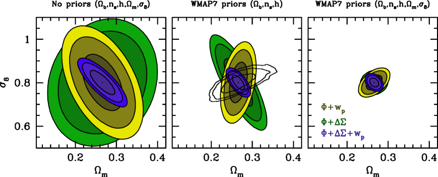
Figure 1: Cosmological constraints in the $\Omega_{\rm m}-\sigma_{8}$ plane that can be obtained by analysing available SDSS measurements of the luminosity function ($\Phi$), galaxy-galaxy lensing signal ($\Delta\Sigma$) and the projected clustering measurements ($w_{\rm p}$). The 68, 95 and 99 percent confidence levels shown by green, yellow and blue contours correspond to the constraints possible when only the $\Phi$ and $\Delta\Sigma$ data are analysed, when only $\Phi$ and $w_{\rm p}$ data are used, and when all three $\Phi$, $\Delta\Sigma$ and $w_{\rm p}$ data are used in conjunction, respectively. The three panels correspond to different priors assumed on the cosmological parameters as indicated at the top of each panel. Note that, in addition to all the CLF parameters and other secondary cosmological parameters, we have also marginalized over the nuisance parameters of our model, ${\eta}$ and $\psi$. The dotted contours in the middle panel show the 68, 95 and 99 percent confidence levels obtained by WMAP7.

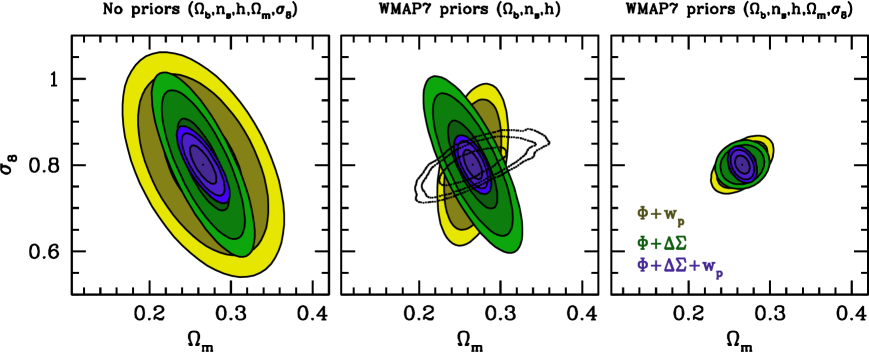
Figure 2: Same as Fig. 1, except for the assumption that the galaxy-galaxy lensing signal ($\Delta\Sigma$) has been measured upto large scales ($\sim 30\,\>h^{-1}{\rm{Mpc}}$) and is modelled using our analytical framework.

As is evident from Eq. (30), the Fisher information matrix is a (weighted) summation over the derivatives of the model predictions, ${\boldsymbol{\mu}}$, with respect to the model parameters, ${\boldsymbol{\theta}}$. The constraining power of any given datapoint on a particular parameter depends on the ratio of the corresponding derivative to the errorbar on this datapoint. The larger the absolute value of this ratio, the greater the constraining power. Since we assume that the errorbars are a certain fixed percentage of the observables themselves (see Table 3), we are interested in the logarithmic derivatives of the observables with respect to the model parameters. These derivatives give insight into the power with which each observable is able to constrain the model parameter of interest. The logarithmic derivatives of the luminosity function, projected galaxy clustering and the galaxy-galaxy lensing signal are presented in Appendix A, together with a detailed discussion.

Throughout this paper, we assume that the covariance matrix for the luminosity function and the galaxy-galaxy lensing signal is diagonal and calculate the Fisher information matrix by using Equation 30. For the galaxy clustering data, we assume that the errorbars are correlated in a manner which is quantitatively equal to the correlations that exist in the measurements of the projected clustering of SDSS galaxies carried out by Zehavi et al. (2011). We make use of Eq. (29) to calculate the Fisher information matrix for the galaxy clustering data.

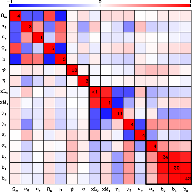
Figure 3: Expected cross-correlation coefficients between different model parameters when the luminosity function, galaxy clustering and galaxy-galaxy lensing signal are analysed together. Red corresponds to perfectly correlated constraints on the corresponding parameters, while blue corresponds to perfectly anti-correlated constraints. The number on the diagonal shows the percentage accuracy with which the corresponding parameter can be constrained.

4 Parameter constraints and covariances

In this section, we forecast the accuracies with which constraints on cosmological parameters can be obtained given the accuracy of the current datasets. To obtain these bounds, we first calculate the Fisher information matrix, $\tilde{F}_{ij}$, by varying the parameters listed in Tables 1 and 2. We calculate the Fisher matrix separately for each of the datasets. As each of the datasets is independently measured, the Fisher information matrix is additive. The inverse of the Fisher matrix gives the covariance matrix, ${\cal C}$, and the diagonal elements of this covariance matrix, ${\cal C}_{ii}$, represents the accuracy with which the $i$-th parameter can be constrained after marginalizing over the other parameters. In Appendix B, we present the procedure we use to obtain 68, 95 and 99 percent confidence ellipses in a plane corresponding to two parameters. In addition to these constraints, we also forecast the cross-correlation coefficients, ${\varrho}_{ij}$, that are expected between the different parameters of our model. We define this coefficient according to the following equation,

$${\varrho}_{ij}=\frac{{\cal C}_{ij}}{\sqrt{{\cal C}_{ii}{\cal C}_{jj}}}\,.$$ (31)

The cross-correlation coefficient is a number that ranges from [-1,1] and captures the degeneracies inherent in the determination of the parameters from the dataset. A positive (negative) cross-correlation coefficient, ${\varrho}_{ij}$, implies that the $i$-th and $j$-th parameters are degenerate, such that the effect of increasing one parameter can be compensated by increasing (decreasing) the other, after allowing the other parameters to readjust to the change (which is the essence of marginalization). A value close to zero implies that the corresponding parameters are only weakly correlated.

4.1 Model A: Vanilla $\Lambda$CDM

We first consider the vanilla $\Lambda$CDM model, in which the Universe is assumed to have a flat geometry, neutrino mass is assumed to be negligible, the initial power spectrum is assumed to be a single power-law, and dark energy is modelled as Einstein’s cosmological constant (i.e., has an EoS with parameter $w_{0}=-1$). In order to assess the impact of priors on the cosmological constraints, we perform three sets of analyses. For the first set, we assume non-informative priors for the CLF parameters and all of the cosmological parameters. For the second set, we include prior information about the secondary cosmological parameters $\Omega_{\rm b}$, $n_{\rm s}$ and $h$ from the seven year analysis of the cosmic microwave background data from WMAP (Komatsu et al., 2011, hereafter WMAP7). For the third set, we additionally include priors on the cosmological parameters $\Omega_{\rm m}$ and $\sigma_{8}$ from WMAP7. We denote the second set of priors to be the fiducial for model A and note that this set will be used in Paper III to obtain the constraints from actual data.

The constraints on the cosmological parameters $\Omega_{\rm m}$ and $\sigma_{8}$ resulting from the three different sets of priors are shown in Fig. 1 after marginalizing over all CLF parameters, two nuisance parameters, ${\eta}$ and $\psi$, and the secondary cosmological parameters, $\Omega_{\rm b}$, $n_{\rm s}$ and $h$. The green contours show the 68, 95 and 99 percent confidence regions that can be obtained using a combination of the luminosity function and the galaxy-galaxy lensing data. In the absence of prior information on the secondary cosmological parameters, the two data sets do not yield particularly tight constraints on $\Omega_{\rm m}$ and $\sigma_{8}$. This is expected in part because the galaxy-galaxy lensing signal measured from SDSS lacks information from large scales ($r_{\rm p}\lower 3.01385pt\hbox{$\;\buildrel>\over{\sim}\;$}2\>h^{-1}{\rm{Mpc}}$). As is evident from the middle panel of Fig. 1, using prior information on the secondary cosmological parameters from WMAP7 significantly reduces the uncertainties on $\Omega_{\rm m}$ and $\sigma_{8}$, although a strong degeneracy of the form $\sigma_{8}\propto\Omega_{\rm m}^{-3.8}$ remains.

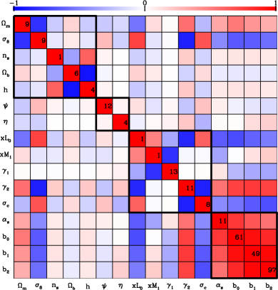
Figure 4: Same as Fig. 3, except when only the luminosity function and the excess surface density data are analysed.

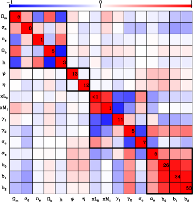
Figure 5: Same as Fig. 3, except when only the luminosity function and the projected galaxy clustering data are analysed.

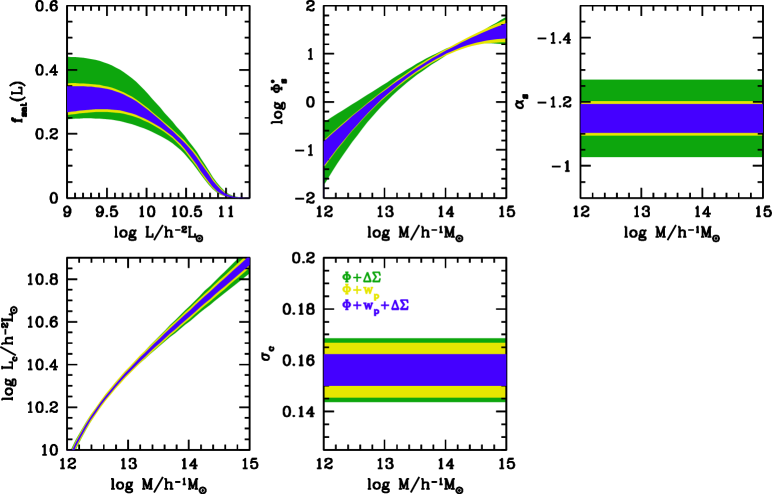
Figure 6: Expected constraints (68 percent confidence) on the satellite fraction, the satellite CLF normalization, its faint end slope, the luminosity-mass relation for centrals and the scatter in this relation using the combination of datasets indicated in the legend.

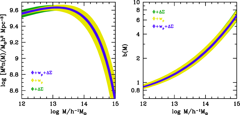
Figure 7: Expected constraints (68 percent confidence) on the mass function and the bias function using the combinations of datasets indicated in the legend.

The confidence regions highlighted in yellow are a result of using a combination of the luminosity function and the clustering data. The constraints without the prior information on secondary parameters (left-hand panel) are significantly better than in the previous case. This is primarily due to the fact that the clustering data extend out to larger radii than the lensing data. As shown in Appendix A, the clustering data on large scales (where the 2-halo term dominates), has good constraining power for $\Omega_{\rm m}$ and $\sigma_{8}$. Addition of the prior information on the secondary cosmological parameters from WMAP7 further improves the constraints (middle panel of Fig. 1). Interestingly, the degeneracies obtained using the luminosity function and the clustering are in an opposite direction to the degeneracies obtained using the luminosity function and the galaxy-galaxy lensing signal, with $\sigma_{8}\propto\Omega_{\rm m}^{11.2}$. This immediately suggests that using the luminosity function in combination with both clustering and lensing will be able to yield even tighter constraints.

The contours highlighted in blue show the combined constraints possible when all three observables are analysed together. Even in the absence of informative priors on the secondary cosmological parameters, $\Omega_{\rm m}$ and $\sigma_{8}$ can already be constrained to very good accuracy, competitive with current constraints in the existing literature (see discussion below). In particular, the constraints on $\Omega_{\rm m}$ and $\sigma_{8}$ from a joint model outperform those obtained by a post-combination of constraints from each of the dataset analysed separately. A joint analysis is able to effectively constrain the CLF parameters, which is crucial for teasing out the tightest possible constraints on the cosmological parameters. This underscores the importance of having each of these observables measured from a single uniform survey. For comparison, the dotted contours in the middle panel of Fig. 1 show the constraints on $\Omega_{\rm m}$ and $\sigma_{8}$ from the WMAP7 analysis of the cosmic microwave background anisotropies. Note that these constraints are very comparable (in magnitude) to what is achievable using our analysis, albeit with roughly orthogonal degeneracies (cf. blue contours in left-hand panel). When using the WMAP7 priors on the secondary cosmological parameters, the constraints on $\Omega_{\rm m}$ and $\sigma_{8}$ from the combination of luminosity function, clustering and galaxy-galaxy lensing using present-day data from SDSS become much tighter than those from WMAP7 alone. Including the WMAP7 priors on $\Omega_{\rm m}$ and $\sigma_{8}$ results in the constraints shown in the right-hand panel of Fig. 1. Because the degeneracies on $\Omega_{\rm m}$ and $\sigma_{8}$ from WMAP7 are roughly orthogonal to those resulting from our analysis, the combination results in extremely tight constraints, even when excluding, for example, the lensing or clustering data.

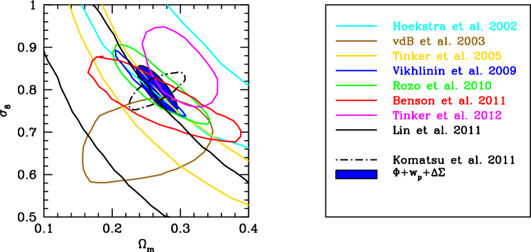
Figure 8: Comparison of the constraints (68 percent confidence) on $\Omega_{\rm m}$ and $\sigma_{8}$ possible from our joint analysis of the luminosity function, galaxy clustering and galaxy-galaxy lensing (shown as a blue shaded region and does not include any prior information on the secondary cosmological parameters) with existing constraints on these parameters from a number of independent methods, such as, abundance of massive clusters (Vikhlinin et al., 2009; Rozo et al., 2010; Benson et al., 2011), cosmic shear measurement (Hoekstra et al., 2002; Lin et al., 2011) and halo occupation distribution modelling of galaxy clustering (van den Bosch et al., 2003; Tinker et al., 2005, 2012). The WMAP7 constraints are shown using dot-dashed contours.

As indicated earlier, the galaxy-galaxy lensing data that we are using to forecast the cosmological constraints only extend to projected spatial scales of $2\>h^{-1}{\rm{Mpc}}$. In Fig. 2, we explore how the constraints on $\Omega_{\rm m}$ and $\sigma_{8}$ would improve if the galaxy-galaxy lensing was also measured and modelled on scales of about $30\,\>h^{-1}{\rm{Mpc}}$. Such measurements would be available in the near future using data from the SDSS (U. Seljak, private communication). A comparison of these constraints with those shown in Fig. 2, shows that the largest improvement corresponds to the case where we obtain cosmological constraints by combining the luminosity function and the galaxy-galaxy lensing data without any priors from WMAP7. However, when using the fiducial set of priors on the secondary cosmological parameters (or the full set of priors from WMAP7), the constraints on $\Omega_{\rm m}$ and $\sigma_{8}$ are expected to improve only marginally.

In Fig. 3, we show the cross-correlation coefficients for our model parameters expected from a joint analysis of the luminosity function, galaxy clustering and galaxy-galaxy lensing and using the fiducial prior set. Squares coloured in red (blue) indicate the presence of a positive (negative) cross-correlation coefficient. Squares devoid of colour indicate a cross-correlation coefficient close to zero. The number on the diagonal squares is the percentage accuracy (rounded to the nearest integer) with which the corresponding parameter can be constrained after marginalizing over all other parameters. The first five parameters are the cosmological parameters, the next two are the nuisance parameters, followed by the five central CLF parameters and finally the 4 satellite CLF parameters complete the set. Of the CLF parameters, x$L_{0}$, x$M_{1}$, $\gamma_{2}$ and $\sigma_{c}$, which describe the normalizations, the high mass end slope and the scatter of the $\tilde{L_{\rm c}}(M)$ relation are the parameters with constraints that are better than $\sim 4$ percent. The familiar degeneracy between x$L_{0}$ and x$M_{1}$ is manifested by a positive cross-correlation coefficient (see Appendix A). In general, the central CLF parameters are very tightly coupled with each other and show a number of degeneracies. The same is true for the satellite CLF parameters. In particular the parameters $b_{0}$, $b_{1}$ and $b_{2}$ that describe the normalization, $\Phi_{*}(M)$, are constrained very poorly and in a highly correlated fashion. There is also a non-negligible cross-talk between the central CLF parameters, satellite CLF parameters and the nuisance parameters.

However, this figure clearly shows that the cross-correlation matrix nicely separates out into a block diagonal form. Most importantly, the block of the cosmological parameters is found to have only weak correlations with the blocks of CLF parameters and nuisance parameters. This implies that the constraints on the cosmological parameters are fairly robust to details regarding the modelling of the halo occupation statistics. This is in contrast with Fig. 4, where we show the cross-correlation matrix expected from the combination of the luminosity function and the currently existing galaxy-galaxy lensing data. This combination shows significant degeneracies between the cosmological parameters and a number of CLF parameters. These degeneracies are suppressed by using the combination of the luminosity function and the galaxy clustering data, as can be seen from Fig. 5. Analyzing all the three data sets together further improves the constraints on $\Omega_{m}$ and $\sigma_{8}$.

One of the significant cross-correlation between parameters from the cosmological block and the other parameters, when all the three datasets are analysed together, is between $\sigma_{8}$ and the nuisance parameter ${\eta}$, which characterizes the uncertainty in the calibration of the normalization of the concentration-mass relation. This degeneracy is a manifestation of the well-known fact that the normalization of the concentration-mass relation depends on $\sigma_{8}$: dark matter haloes in a universe with a larger value of $\sigma_{8}$ collapse earlier, when the universe is denser, and therefore have higher concentrations (e.g., Macciò et al., 2008). Hence, an increase in $\sigma_{8}$ can be countered by a decrease in ${\eta}$, which explains why the cross correlation coefficient is negative.

We also expect to obtain excellent constraints on the halo occupation distribution of galaxies from our analysis. The upper panels of Fig. 6 show the constraints, using the fiducial prior set, on the satellite fractions as a function of luminosity and the normalization and faint-end slope of the satellite CLF as a function of halo mass, respectively, for different combinations of data, as indicated in the legend. The bottom panels show the constraints on the average halo mass-luminosity relationship of central galaxies and its scatter. It is clear that the combination of luminosity function and clustering outperforms the combination of the luminosity function and the galaxy-galaxy lensing signal in constraining the halo occupation distribution parameters, and the constraints improve only marginally when analysing all three datasets together. The importance of a joint analysis, however, is very clear from Figure 7, which shows the expected accuracy with which the halo mass function and the halo bias function can be constrained. These two quantities are the primary source of our cosmological information. The constraints on these quantities are fairly broad when the galaxy-galaxy lensing data are left out, especially at the high mass end. However, they improve considerably with the inclusion of the galaxy-galaxy lensing data.

Finally, in Fig. 8, we compare the constraints on $\Omega_{\rm m}$ and $\sigma_{8}$ possible from our joint analysis with existing constraints from other independent studies using a variety of observations. To avoid excessive overcrowding in the figure, we only show the 68 percent confidence regions from each study. As representative of the cosmic shear studies, we show results from Hoekstra et al. (2002) using cyan contours and the latest analysis of the SDSS Stripe 82 co-added data by Lin et al. (2011) using black contours. Clearly, the current data on cosmic shear measurements is not yet able to put interesting constraints on $\Omega_{\rm m}$ and $\sigma_{8}$. However, this situation is expected to improve drastically in the near future, thanks to a number of deep, large-scale photometric surveys planned for this decade. More stringent constraints on $\Omega_{\rm m}$ and $\sigma_{8}$ have come from studies of cluster abundances. As representative of these studies, we show the constraints obtained by Vikhlinin et al. (2009) using X-ray clusters from the Chandra Cluster Cosmology Project (blue contours), by Rozo et al. (2010) using optically selected MaxBCG clusters (green contours), and by Benson et al. (2011) using SZ-selected clusters from the South Pole Telescope (red contours).

On this compilation plot, we also show the constraints obtained by two studies that used halo occupation modeling to study the abundances and clustering of galaxies. van den Bosch et al. (2003) used the observed abundance and luminosity dependence of the correlation length of 2dFGRS galaxies, combined with independent constraints on the mass-to-light ratios of galaxy clusters, which resulted in the constraints depicted by the brown contours. Using a similar method, Tinker et al. (2005) modelled the small-scale clustering of SDSS galaxies and used the mass-to-light ratio on cluster scales to obtain the constraints depicted in orange.

More recently, Tinker et al. (2012) analysed the small scale ($<3\,\>h^{-1}{\rm{Mpc}}$) clustering of galaxies from SDSS and the mass-to-number ratio of the maxBCG cluster sample (as obtained from the weak lensing analysis of Sheldon et al., 2009) to constrain $\Omega_{\rm m}$ and $\sigma_{8}$. The 68 percent confidence contours from their analysis are shown using magenta contours. When compared to the forecasted constraints from our analysis (shown as a shaded region and including no prior information about the secondary cosmological parameters), it is clear that modelling the entire galaxy-galaxy lensing signal, rather than just using the mass-to-number ratio, yields additional information about the cosmological parameters. The fact that the clustering and lensing samples used by Tinker et al. (2012) are not well-matched (the clustering data is taken from the spectroscopic SDSS, whose median redshift is very different from that of the photometric sample used to create the maxBCG cluster catalog) also introduces additional systematics which result in the weaker constraints shown in the figure.

Note that all these different constraints use different priors on the secondary cosmological parameters (or none). Therefore their merits cannot be compared directly. However, this figure does demonstrate that the joint analysis of the abundances, clustering and lensing of galaxies, as advocated in this paper, is an extremely powerful way of constraining the parameters, $\Omega_{\rm m}$ and $\sigma_{8}$. Such an analysis is forecast to yield constraints, even without any additional priors on the secondary cosmological parameters, that are competitive, if not better than, any of the previous constraints, including the WMAP7 data itself.

4.2 Model B: Massive Neutrinos

Next we consider cosmological models with massive neutrinos. We retain the assumption of a flat Universe and the standard dark energy EoS, $w_{0}=-1$. We assume uninformative priors on the CLF parameters and the primary cosmological parameters of interest, $\Omega_{\rm m}$, $\sigma_{8}$ and $\Omega_{\nu}$. The secondary cosmological parameters have priors from the 7-year WMAP data analysis. The density parameter $\Omega_{\nu}$ is related to the mass of the neutrino species, $m_{\nu}$ such that

$$\Omega_{\nu}h^{2}=\frac{\sum_{i}m_{\nu,i}}{94{~{}\rm eV}}\,.$$ (32)

We perform the Fisher analysis around the cosmological parameters for model B displayed in Table 1. The fiducial value for the neutrino density parameter is assumed to be $\Omega_{\nu}=0.004$ which corresponds to $\sum m_{\nu}=0.184\,{\rm e}{\rm V}$.

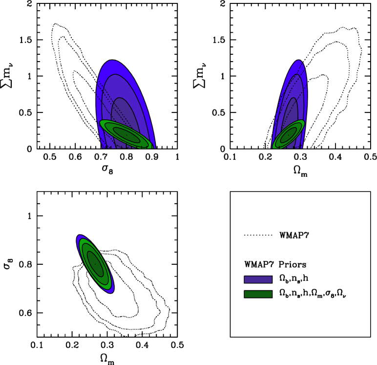
Figure 9: The 68, 95 and 99 percent confidence constraints on the parameters $\sum m_{\nu}$, $\sigma_{8}$ and $\Omega_{\rm m}$ after marginalizing over the CLF parameters and other nuisance parameters in our model for two different priors as indicated in the legend. The confidence contours from the WMAP7 analysis are shown using dotted lines.

The presence of massive neutrinos in the Universe affects the matter power spectrum primarily by suppressing the density fluctuations on scales smaller than the neutrino free streaming scale. We use the framework of Eisenstein & Hu (1999) to obtain the linear power spectrum of matter fluctuations in the presence of massive neutrinos. Kiakotou et al. (2008) have suggested a minor modification to this fitting function which leads to a more accurate prediction of the linear power spectrum when the number of neutrino species with degenerate masses $N_{\nu}=3$. We use this modification to get the linear power spectrum of matter fluctuations. When computing the non-linear matter power spectrum, and the halo mass and bias functions from the linear theory matter power spectrum, we assume that the calibrations which fit the standard $\Lambda$CDM simulations also generalize to the cosmological models that include massive neutrinos. In particular, we assume that the non-linear power spectrum is obtained from the linear power spectrum using the HALOFIT prescription given by Smith et al. (2003) with the modifications suggested recently by Bird et al. (2012) based upon numerical simulations including massive neutrinos, and that the dependence of the halo mass and bias functions on the linear matter power spectrum is given by parameters calibrated by Tinker et al. (2008). In addition, we also assume that the density distribution in halos follows the NFW profile with the concentration-mass relation given by the calibration obtained by Macciò et al. (2007).

The constraints on the parameters $\Omega_{\rm m}$, $\sigma_{8}$ and the sum of massive neutrinos that can be obtained from a joint analysis of the abundance, clustering and weak lensing of galaxies are shown in Fig. 9. The blue contours represent constraints when using the fiducial set of priors on the secondary cosmological parameters. As before, we have marginalized over all the CLF parameters, the nuisance parameters and the other cosmological parameters. The addition of the parameter, $\sum m_{\nu}$, as expected, leads to more freedom for $\Omega_{\rm m}$ and $\sigma_{8}$ and this slightly weakens the constraints in the $\Omega_{\rm m}-\sigma_{8}$ plane compared to model A. The expected error on the sum of neutrinos is not small enough to rule out the massless neutrino case (if at least, as assumed here, the true sum of neutrino masses is $\sum m_{\nu}=0.184\,\>{\rm eV}$). The dotted contours show the results from the analysis of the WMAP7 data. It is clear that both analyses on their own allow values for the sum of neutrino masses as high as 1 eV at 95 percent confidence. However, the cosmic microwave background data, in such a scenario, requires a very low value for $\sigma_{8}\,\sim\,0.6$. Our analysis can rule out such values of $\sigma_{8}$ at very high confidence. This shows that combining the constraints from our analysis with the cosmic microwave background results can certainly provide a significantly better upper limit on the sum of neutrino masses. This, in essence, is very similar to how the addition of cluster abundances constraints improves the constraints on neutrino masses from the WMAP7 analysis (e.g., Benson et al., 2011).

The green confidence contours shown in Fig. 9 represent the constraints on $\Omega_{\rm m}$, $\sigma_{8}$ and $\sum m_{\nu}$ possible from our analysis when using all prior information available from WMAP7. If the sum of neutrino masses is truly as large as we have assumed in our analysis, such a combination will allow the tantalising possibility of the first signs of detection of a non-zero sum of neutrino masses at $\sim 3\sigma$ confidence.

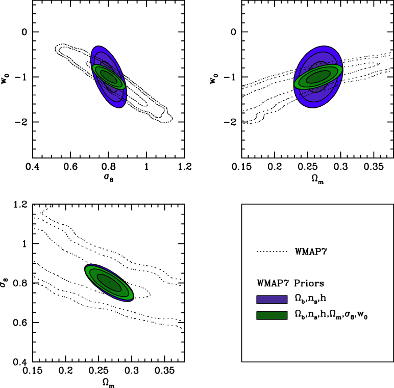
Figure 10: The 68, 95 and 99 percent confidence constraints on the parameters $w_{0}$, $\sigma_{8}$, $\Omega_{\rm m}$ from our analysis after marginalizing over the CLF parameters and other nuisance parameters in our model for two different priors as indicated in the legend. The confidence contours from the WMAP7 analysis are shown using dotted lines.

4.3 Model C: Dark Energy Equation of State

Finally, we focus on models with a modified EoS for the dark energy, i.e., with $w_{0}\neq 1$. For these models, we restore the assumption of massless neutrinos and we maintain the assumption of a flat Universe. Modifications to the dark energy EoS change the expansion history of the Universe and the growth rate of structure formation. The expansion factor $E(z)$ is given by

$$E(z)=[\Omega_{\rm m}\,(1+z)^{3}+\Omega_{\Lambda}\,(1+z)^{3(1+w_{0})}]^{1/2}\,,$$ (33)

whereas the dependence of the growth factor on redshift can be calculated by solving the second order differential equation obtained by combining the continuity and Euler equations in the linear regime (see Mo et al. 2010),

$$\ddot{g}+2\,H\,\dot{g}=\frac{3}{2}\Omega_{\rm m}\,H_{0}^{2}\,(1+z)^{3}\,g\,.$$ (34)

Changing the variables from time to $\eta=\ln a(t)$, this equation can be written as

$$g^{\prime\prime}+\left[2+\frac{d\ln E}{d\eta}\right]g^{\prime}=\frac{3}{2E^{2}(\eta)}\Omega_{\rm m}(1+z)^{3}\,,$$ (35)

where a dash indicates a derivative with respect to $\eta$. We use the following two boundary conditions to solve for the growth factor: (a) $g(a=0.001)=1$ and (b) $g^{\prime}(a=0.001)=1$, consistent with the expectation that $g\propto a$ in the matter-dominated era. We renormalize the scale factor to equal unity at redshift $z=0$, once the solution has been found.

These changes to the growth factor that arise from having the dark energy EoS differ from $w_{0}=-1$ propagate in the redshift evolution of the linear matter power spectrum, and thereby affect the halo mass function, the halo bias function and the mass dependence of the concentration parameter that describes the density profile of dark matter haloes. These changes cause the galaxy abundance, the galaxy clustering and the galaxy-galaxy lensing signal to deviate from the ‘standard’ vanilla-$\Lambda$CDM predictions. We once again assume that the calibrations required to compute the non-linear matter power spectrum, the halo mass function, the halo bias function and the halo concentrations from the linear theory power spectrum are the same as in the standard $\Lambda$CDM case.

The constraints on the dark energy EoS and the cosmological parameters $\Omega_{\rm m}$ and $\sigma_{8}$ that are achievable from our joint analysis, using the WMAP7 priors on the secondary cosmological parameters, are shown in Fig. 10. The dotted lines represent the 68, 95 and 99 percent confidence intervals from the WMAP7 data, and are shown for comparison. Note that our analysis results in degeneracies that are very similar to those from the WMAP7 analysis, whereby an increase in $\sigma_{8}$ can compensate a decrease in the value of $w_{0}$. The slight differences in the degeneracy directions, however, allow tighter constraints when combining both data sets. The resulting confidence intervals are shown using green contours.

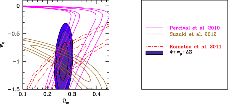
Figure 11: Comparison of the constraints (68, 95 and 99 percent confidence) on $\Omega_{\rm m}$ and $w_{0}$ possible from our joint analysis of the luminosity function, galaxy clustering and galaxy-galaxy lensing (shown as a shaded region and includes WMAP7 priors on secondary cosmological parameters) with existing constraints on these parameters. The magenta contours are from the analysis of the baryon acoustic feature from SDSS data by Percival et al. (2010), the brown contours are from the analysis of SNeIa data by Suzuki et al. (2012) and the red contours are from the analysis of WMAP7 data by Komatsu et al. (2011).

In Fig. 11, we compare the constraints on $\Omega_{\rm m}$ and $w_{0}$ that can be obtained from our joint analysis with those obtained from other cosmological probes. Supernovae of Type Ia (SNeIa) and measurements of the baryon acoustic feature (BAF) in the clustering of galaxies can be used as standard candles and standard rulers, respectively, in order to map the expansion history of the Universe as a function of redshift. Brown contours indicate the 68, 95 and 99 percent confidence intervals on the parameters $\Omega_{\rm m}$ and $w_{0}$ obtained by Suzuki et al. (2012) from the Union2.1 compilation of SNeIa. The constraints obtained by Percival et al. (2010), who measured the BAF by combining SDSS and 2dFGRS data are shown using magenta contours, while the constraints from the analysis of the WMAP7 data are shown using red contours. Each of these constraints have severe degeneracies in the $\Omega_{\rm m}-w_{0}$ plane, but are very powerful when used in conjunction. The constraints forecast for our analysis, shown using filled blue contours, indicates that our results will be degenerate in yet another direction and can therefore significantly add to our knowledge of the cosmological parameters $\Omega_{\rm m}$ and $w_{0}$. It is worth mentioning that unlike our analysis, the probes of expansion history such as SNe1a are insensitive to the parameter $\sigma_{8}$. The overall amplitude of the clustering measurements used to detect the BAF does depend upon $\sigma_{8}$, but cannot be used to constrain it, due to its degeneracy with the value of galaxy bias. Our analysis, on the other hand, is able to constrain both $\sigma_{8}$ and galaxy bias simultaneously due to our modelling of small scale clustering and the galaxy-galaxy lensing signal (see also Seljak et al., 2005).

5 Summary

The distribution of galaxies, which is routinely mapped out by large scale galaxy surveys, contains a wealth of information about the cosmological parameters. Unfortunately, harvesting this information is not straightforward because galaxies are biased tracers of the matter distribution. We have presented a powerful method that can be used to simultaneously solve for both the cosmological parameters as well as the galaxy bias. Our method relies on an accurate halo occupation distribution modelling of galaxy abundances, galaxy clustering and galaxy-galaxy lensing, which probes scales well into the non-linear regime of structure formation.

In Paper I we developed an analytical framework to predict each of these observables, given a cosmology and the CLF parameters that describe the halo occupation statistics of galaxies. In this paper, we have presented the strength of each of these observables (see Appendix A) to constrain our model parameters. We have also performed a Fisher matrix analysis for a standard $\Lambda$CDM cosmology with flat geometry. We primarily focused on the cosmological parameters $\Omega_{\rm m}$ and $\sigma_{8}$, and treated the other cosmological parameters ($\Omega_{\rm b}$, $n_{\rm s}$ and $h$) as secondary parameters, for which we adopted priors taken from the seven year analysis of the WMAP data.

We have shown that an analysis of the luminosity function of galaxies combined with galaxy-galaxy lensing is marred by a number of degeneracies between the CLF parameters and the cosmological parameters, which effectively weakens the cosmological constraints. However, when this analysis is complemented with clustering data, a number of these degeneracies are broken. For the standard $\Lambda$CDM cosmology, we forecast that the constraints on $\Omega_{\rm m}$ and $\sigma_{8}$ that are achievable from our joint analysis, using data that is already available from the SDSS, are of the order of $3$ and $2$ percent, respectively. Such constraints will be competitive with (and complementary to) the tightest constraints that are presently available (see Fig. 8). We will perform such an analysis in Paper III (Cacciato et al, in preparation).

One of the most important results of this paper is the demonstration that the covariance of the posterior distribution of parameters from our joint analysis of the luminosity function, galaxy clustering and galaxy-galaxy lensing has a block diagonal form (see Fig. 3). In particular, the cosmological parameters form a separate block, which is only weakly correlated with the other blocks (2 nuisance parameters, 5 parameters that describe the CLF of central galaxies, and 4 parameters that describe the CLF of satellites). This implies that the cosmological constraints will be robust to uncertainties related to details of the halo occupation statistics, and that we can simultaneously obtain tight constraints on the halo occupation statistics, properly marginalized over the uncertainties in the cosmological parameters.

We have also investigated two extensions of the standard $\Lambda$CDM model. In the first extension we included massive neutrinos in our analysis. We showed that although the constraints on the sum of the neutrino masses, $\sum m_{\nu}$, from our analysis are predicted to be of the order of $1$ eV (at $95$ percent confidence, assuming realistic errors on the data), the degeneracies between $\sum m_{\nu}$ and $\sigma_{8}$ are oriented differently than those from the WMAP7 analysis. Consequently, the combination of our results with those from WMAP7 can significantly improve the constraints on $\sum m_{\nu}$. In particular, we have shown that such an analysis should be able to provide constraints of the order of 0.2 eV at 99 percent confidence.

As a second extension of $\Lambda$CDM, we also allowed for a non-standard EoS for the dark energy, characterized by $w_{0}\neq-1$. We showed that the current data on the abundances, clustering and lensing of galaxies in SDSS is already sufficient to put interesting constraints on $w_{0}$, especially when combined with the WMAP7 data. In particular, the constraints on $w_{0}$ from our analysis are forecast to correspond to $\Delta w_{0}=0.5$ (95 percent confidence, with priors on the secondary cosmological parameters). This further improves to $\Delta w_{0}=0.2$ when using the full prior information available from WMAP7 (see Fig. 10). Since the SDSS data considered here only spans a very narrow range in redshift ($z\lower 3.01385pt\hbox{$\;\buildrel<\over{\sim}\;$}0.2$), there is a huge potential for improvement by measuring the abundances, clustering and lensing of galaxies at higher redshifts.

Finally, we note that although the main focus of our joint analysis is to constrain cosmological parameters, we have also shown that we will be able to obtain a detailed, statistical description of the galaxy-matter connection, as parameterized by the CLF, fully marginalized over uncertainties in the cosmological parameters. In particular, our analysis can provide excellent constraints on the average relation between halo mass and central galaxy luminosity, including its scatter, on the satellite fraction as function of luminosity, and on the conditional luminosity function of satellites. These constraints characterize, among others, the efficiency with which haloes of different masses are able to convert their cosmological share of baryons into stars (i.e., galaxies). This will be of great value to inform models of galaxy formation and evolution. Another powerful application of a tightly constrained CLF is the construction of realistic mock galaxy catalogues (see Paper I for an example). The galaxies in these mock catalogues will, by construction, have abundances, clustering and a cross-correlation with matter, that are all consistent with current data.

6 Acknowledgments

We are grateful to Matthew Becker, Wayne Hu, Alexie Leauthaud, Yin Li, Eduardo Rozo, Jeremy Tinker and Martin White for many interesting discussions and possible extensions of the research described in this paper. SM acknowledges support from the Kavli Institute for Cosmological Physics at the University of Chicago through the NSF grant PHY-0551142 and an endowment from the Kavli Foundation. The analysis presented in this work has been performed on the Joint Fermilab - KICP Supercomputing Cluster, supported by grants from Fermilab, Kavli Institute for Cosmological Physics, and the University of Chicago. FvdB acknowledges support from the Lady Davis Foundation for a Visiting Professorship at Hebrew University. FvdB was also supported in part by the National Science Foundation under Grant No. NSF PHY11-25915.

Appendix A Fisher information matrix

The Fisher information matrix, defined as the (negative of the) second derivative of the log-likelihood surface, can be used to calculate the constraints on the parameters of our model, given the observational data. The Fisher information matrix can be expressed in terms of the derivatives of the observables with respect to the dimensionless parameters $\lambda_{i}$ (see Eqs. 28 and 29). For our analysis, we have assumed that the observational constraints have fixed fractional accuracy. Ignoring the covariance between data points for simplicity, the dimensionless Fisher information matrix is given by

$$\tilde{F}_{ij}=\sum_{k}\frac{1}{f_{\mu,k}^{2}}\left(\frac{\partial\ln\mu_{k}}{\partial\lambda_{i}}\right)\left(\frac{\partial\ln\mu_{k}}{\partial\lambda_{j}}\right)\,,$$ (36)

where $f_{\mu,k}$ is the fractional accuracy of the $k$-th data constraint and $\left[{\partial\ln\mu_{k}}/{\partial\lambda}\right]$ is the logarithmic derivatives of the observable with respect to $\lambda_{i}$. In this appendix, we present the logarithmic derivatives of the luminosity function, the galaxy-galaxy clustering signal and galaxy-galaxy lensing signal with respect to some of our primary model parameters, which enter the Fisher information matrix defined above.

Figure 12: The logarithmic derivatives of the luminosity function with respect to the dimensionless CLF parameter $\lambda$. The CLF parameter corresponding to each logarithmic derivative is indicated at the top of each panel.

Figure 13: The logarithmic derivatives of the luminosity function with respect to the dimensionless cosmological parameters $\lambda$. The cosmological parameter corresponding to each logarithmic derivative is indicated at the top of each panel.

Figure 14: The logarithmic derivatives of the galaxy clustering signal with respect to the dimensionless CLF parameter $\lambda$. Different line types correspond to the six different luminosity bins. The faintest bin is shown using solid line, while the brightest bin is shown using a dot-long-dashed line. The CLF parameter corresponding to each logarithmic derivative is indicated at the top of each panel.

Figure 15: The logarithmic derivatives of the galaxy clustering signal with respect to the dimensionless cosmological parameter $\lambda$. The cosmological parameter corresponding to each logarithmic derivative is indicated at the top of each panel. The different line types correspond to the same bins as that in Fig 14.

Figure 16: The logarithmic derivatives of the galaxy-galaxy lensing signal with respect to the dimensionless CLF parameter $\lambda$. The CLF parameter corresponding to each logarithmic derivative is indicated at the top of each panel. The different line types correspond to the same bins as that in Fig 14.

Figure 17: The logarithmic derivatives of the galaxy-galaxy lensing signal with respect to the dimensionless cosmological parameter $\lambda$. The cosmological parameter corresponding to each logarithmic derivative is indicated at the top of each panel. The different line types correspond to the same bins as that in Fig 14.

We first focus on the logarithmic derivatives of the luminosity function with respect to the central and the satellite CLF parameters, shown in different panels of Fig. 12. The luminosity function of galaxies is always dominated by central galaxies. Therefore it contains more information about the central CLF parameters than the satellite CLF parameters, as is evident from a comparison of the magnitudes of the logarithmic derivatives in panels (a)-(e) with those in panels (f)-(i). If a positive change in a parameter causes central galaxies of the same luminosity to live in lower mass haloes, which are more abundant, it results in an increase in the galaxy luminosity function and it shows up as a positive derivative with respect to that parameter. These logarithmic derivatives with respect to the central CLF parameters are largest at the bright end (except for the parameter $\gamma_{1}$ which controls the low mass end of the halo mass luminosity relation). On the other hand, the logarithmic derivatives with respect to the satellite CLF parameters are largest at the faint end because the fractional contribution of satellite galaxies (satellite fraction) to the luminosity function increases as we go to fainter and fainter galaxies. The luminosity function gives a large amount of information about the parameters $L_{0}$ and $M_{1}$, which determine the pivot points of the $\tilde{L_{\rm c}}(M)$ relation. It is interesting to note that that the derivatives with respect to x$L_{0}$ and x$M_{1}$ are opposite in sign which points to an interesting degeneracy: increasing x$L_{0}$ can be compensated by increasing the parameter x$M_{1}$ if all other parameters are kept fixed.

The cosmological parameters affect the luminosity function by changing the halo mass function. As can be seen from panels (a)-(c) of Fig 13, most of the information about the cosmological parameters comes from the bright end of the galaxy luminosity function. This is expected because the change in the halo mass function due to the cosmological parameters is largest at the most massive end. The derivatives with respect to $\Omega_{\rm m}$ and $\sigma_{8}$ have the same sign and are only slightly different in shape. Hence a positive change in $\Omega_{\rm m}$ can be countered with a negative change in $\sigma_{8}$ and vice versa. The weakest constraints are on the parameter $w_{0}$. The parameter $w_{0}$ mainly affects the luminosity function by changing the growth of structure and thus the power spectrum. We have assumed that the luminosity function is only measured at a single redshift $z=0.1$ from SDSS data, thus the leverage in redshift to propagate changes to the growth of structure are not very large. This results in very weak sensitivity to $w_{0}$.

The logarithmic derivatives of the projected galaxy clustering with respect to the CLF parameters are shown in Fig. 14. On large scales, the clustering of galaxies mainly arises due to the two halo term which is sensitive to the clustering of haloes in which these galaxies reside. Since more massive haloes are more strongly clustered, a change in a parameter which causes galaxies to reside on average in more massive haloes will result in an increase in the clustering of galaxies on large scales. On small scales, the one halo terms (central-satellite and the satellite-satellite) dominate the clustering of galaxies. The satellite distribution in more massive haloes is less concentrated but the number of satellites in these haloes is larger and there are competing effects that can result in changes in the clustering of galaxies in directions opposite to the trend on large scales (see e.g. panel [d]). The trends in the logarithmic derivatives, as shown in Fig. 14, on average show that the small scale clustering of galaxies has the most information about the halo occupation parameters. The galaxies in the brightest bins show a large derivative with respect to the central CLF parameters (barring $\gamma_{1}$ as expected). The satellite CLF parameters that determine the normalization of the satellite CLF are almost equally sensitive to all luminosity bins. The logarithmic derivatives are largest for the parameters x$L_{0}$ and x$M_{1}$. Although the derivatives are opposite in sign, the shapes of these derivatives as a function of scale are quite different from each other, thus providing an avenue to constrain the parameters separately.

Comparisons of the logarithmic derivatives of the galaxy clustering signal with respect to the cosmological parameters, shown in Fig. 15, to the derivatives shown in Fig. 13, give an interesting insight. Unlike the logarithmic derivatives of the luminosity function, the derivatives with respect to $\Omega_{\rm m}$ and $\sigma_{8}$ have opposite signs, which suggests that a combination of the two observables adds a lot of information about these parameters. The derivatives of the galaxy clustering signal with respect to the parameter $\Omega_{\rm m}$ increase on large scales. The parameter $\sigma_{8}$ controls the concentration of dark matter haloes and therefore the distribution of the satellite galaxies. Therefore it affects both the small and the large scales. Galaxy clustering on large scales is also sensitive to the parameter $w_{0}$, because it affects the growth of structure, while on small scales the sensitivity is expected due to the changes to the concentration-mass relation.

The information contained in the galaxy-galaxy lensing signal, as shown by the logarithmic derivatives in Fig. 16 and Fig. 17, is dominated by the one halo terms as the signal has only been measured out to a couple of megaparsecs. The derivatives with respect to the CLF parameters show quite different dependencies on scale compared to the clustering data, with a large amout of information coming from the scales of the order of a megaparsec. Most of the trends are fairly similar to the trends in the logarithmic derivatives of the galaxy-galaxy clustering data and depend upon how the CLF parameters change the halo occupation distribution of galaxies. The logarithmic derivatives with respect to the cosmological parameters show that measuring the galaxy-galaxy signal to larger scales can certainly add more information. We have quantified how the constraints on the cosmological parameters improve by using the galaxy-galaxy lensing measured to $\sim 30\,\>h^{-1}{\rm{Mpc}}$ signal in Section 4.

Appendix B Confidence intervals from the Fisher matrix

The inverse of the Fisher information matrix gives the covariance with which the parameters of the model can be constrained given the data. Here, we briefly present the procedure to obtain the confidence intervals in a two dimensional parameter space given this covariance matrix. Let $P(x,y)$ denote the posterior probability distribution for two parameters of interest $x$ and $y$ after marginalizing over the rest of the parameter set. For simplicity, let us assume that the constraints on these two parameters are uncorrelated, which implies that the subset of the full covariance matrix corresponding to these two parameters is a diagonal matrix given by

$$C=\begin{pmatrix}\sigma^{2}_{xx}&0\\ 0&\sigma^{2}_{yy}\end{pmatrix}.$$ (37)

In case the covariance matrix is not diagonal, one can always diagonalise it by rotating the co-ordinate system and aligning the axes with the eigenvectors of this covariance matrix. Let us assume that the posterior distribution $P(x,y)$ is Gaussian and without loss of generality, let us assume that it is centred at $(0,0)$, such that

$$P(x,y)=\frac{1}{2\pi\,[\sigma_{xx}\sigma_{yy}]}\exp\left(-\left[\frac{x^{2}}{2\sigma_{xx}^{2}}+\frac{y^{2}}{2\sigma_{yy}^{2}}\right]\right)\,.$$ (38)

Changing variables to the dimensionless quantities $\xi^{\prime}$ and $\theta$ defined such that

$$x=\sigma_{xx}\xi^{\prime}\cos(\theta);\,\,y=\sigma_{yy}\xi^{\prime}\sin(\theta)\,,$$ (39)

gives

$$P(x,y)\,{\rm d}x\,{\rm d}y = P(\xi^{\prime},\theta){\rm d}\xi^{\prime}\,{\rm d}\theta\,,$$ (40)

$$= \frac{\xi^{\prime}\,{\rm d}\xi^{\prime}\,{\rm d}\theta}{2\pi}\,\exp\left(\frac{-\xi^{\prime 2}}{2}\right)\,.$$ (41)

The probability that the true model lies within a region enclosed by the iso-probability contour $\xi$ is then given by

$$P_{\xi}=\int_{0}^{2\pi}\int_{0}^{\xi}P(\xi^{\prime},\theta)\,{\rm d}\xi^{\prime}\,{\rm d}\theta=1-\exp\left[\frac{-\xi^{2}}{2}\right]\,.$$ (42)

The iso-probability contours $\xi=1.5096$, $2.4477$ and $3.0349$ correspond to $P_{\xi}=0.68$, $0.95$ and $0.99$, respectively. These values of $\xi$ correspond to 68, 95 and 99 percent confidence ellipses in the $x-y$ plane with principal axes of length equal to $\xi\sigma_{xx}$ and $\xi\sigma_{yy}$.

To summarize, the step-by-step procedure we use to obtain the confidence ellipses is as follows: (i) invert the entire $n_{\rm par}\times n_{\rm par}$ Fisher matrix to obtain the covariance matrix, (ii) choose the $2\times 2$ subset of the covariance matrix corresponding to the two parameters of interest, (iii) find the eigenvalues and eigenvectors of this submatrix, (iv) draw 68, 95 and 99 percent confidence ellipses with the axes aligned to the eigenvectors, and with axes lengths equal to $1.5096$, $2.4477$ and $3.0349$ times the square root of the corresponding eigenvalues found in step (iii), respectively. Note that, this procedure can be trivially generalized to obtain confidence ellipsoids in a subspace spanned by any number of parameters.

References

- Abazajian et al. (2009) Abazajian, K. N., Adelman-McCarthy, J. K., Agüeros, M. A., et al. 2009, ApJS, 182, 543
- Anderson et al. (2012) Anderson, L., Aubourg, E., Bailey, S., et al. 2012, ArXiv e-prints
- Baldauf et al. (2010) Baldauf, T., Smith, R. E., Seljak, U., & Mandelbaum, R. 2010, Physical Review D, 81, 063531
- Baldry et al. (2008) Baldry, I. K., Glazebrook, K., & Driver, S. P. 2008, MNRAS, 388, 945
- Benson et al. (2011) Benson, B. A., de Haan, T., Dudley, J. P., et al. 2011, ArXiv e-prints
- Berlind & Weinberg (2002) Berlind, A. A. & Weinberg, D. H. 2002, ApJ, 575, 587
- Bird et al. (2012) Bird, S., Viel, M., & Haehnelt, M. G. 2012, MNRAS, 420, 2551
- Blake et al. (2011) Blake, C., Davis, T., Poole, G. B., et al. 2011, MNRAS, 415, 2892
- Blanton et al. (2003a) Blanton, M. R., Brinkmann, J., Csabai, I., et al. 2003a, AJ, 125, 2348
- Blanton et al. (2003b) Blanton, M. R., Hogg, D. W., Bahcall, N. A., et al. 2003b, ApJ, 592, 819
- Cacciato et al. (2009) Cacciato, M., van den Bosch, F. C., More, S., et al. 2009, MNRAS, 394, 929
- Cole et al. (2001) Cole, S., Norberg, P., Baugh, C. M., et al. 2001, MNRAS, 326, 255
- Colless et al. (2001) Colless, M., Dalton, G., Maddox, S., et al. 2001, MNRAS, 328, 1039
- Coupon et al. (2011) Coupon, J., Kilbinger, M., McCracken, H. J., et al. 2011, ArXiv e-prints
- Demleitner et al. (2001) Demleitner, M., Accomazzi, A., Eichhorn, G., et al. 2001, in Astronomical Society of the Pacific Conference Series, Vol. 238, Astronomical Data Analysis Software and Systems X, ed. F. R. Harnden, Jr., F. A. Primini, & H. E. Payne, 321
- Dunkley et al. (2011) Dunkley, J., Hlozek, R., Sievers, J., et al. 2011, ApJ, 739, 52
- Eisenstein & Hu (1999) Eisenstein, D. J. & Hu, W. 1999, ApJ, 511, 5
- Eisenstein et al. (2005) Eisenstein, D. J., Zehavi, I., Hogg, D. W., et al. 2005, ApJ, 633, 560
- Guy et al. (2010) Guy, J., Sullivan, M., Conley, A., et al. 2010, A&A, 523, A7
- Hoekstra et al. (2002) Hoekstra, H., Yee, H. K. C., & Gladders, M. D. 2002, ApJ, 577, 595
- Huff et al. (2011) Huff, E. M., Eifler, T., Hirata, C. M., et al. 2011, ArXiv e-prints
- Jing et al. (1998) Jing, Y. P., Mo, H. J., & Boerner, G. 1998, ApJ, 494, 1
- Kaiser (1987) Kaiser, N. 1987, MNRAS, 227, 1
- Kessler et al. (2009) Kessler, R., Becker, A. C., Cinabro, D., et al. 2009, ApJS, 185, 32
- Kiakotou et al. (2008) Kiakotou, A., Elgarøy, Ø., & Lahav, O. 2008, Physical Review D, 77, 063005
- Komatsu et al. (2011) Komatsu, E., Smith, K. M., Dunkley, J., et al. 2011, ApJS, 192, 18
- Kowalski et al. (2008) Kowalski, M., Rubin, D., Aldering, G., et al. 2008, ApJ, 686, 749
- Leauthaud et al. (2012) Leauthaud, A., Tinker, J., Bundy, K., et al. 2012, ApJ, 744, 159
- Li et al. (2007) Li, Y., Mo, H. J., van den Bosch, F. C., & Lin, W. P. 2007, MNRAS, 379, 689
- Lin et al. (2011) Lin, H., Dodelson, S., Seo, H.-J., et al. 2011, ArXiv e-prints
- Lueker et al. (2010) Lueker, M., Reichardt, C. L., Schaffer, K. K., et al. 2010, ApJ, 719, 1045
- Macciò et al. (2008) Macciò, A. V., Dutton, A. A., & van den Bosch, F. C. 2008, MNRAS, 391, 1940
- Macciò et al. (2007) Macciò, A. V., Dutton, A. A., van den Bosch, F. C., et al. 2007, MNRAS, 378, 55
- Mandelbaum et al. (2006) Mandelbaum, R., Seljak, U., Kauffmann, G., Hirata, C. M., & Brinkmann, J. 2006, MNRAS, 368, 715
- Mantz et al. (2010) Mantz, A., Allen, S. W., Rapetti, D., & Ebeling, H. 2010, MNRAS, 406, 1759
- Massey et al. (2007) Massey, R., Rhodes, J., Leauthaud, A., et al. 2007, ApJS, 172, 239
- Mo et al. (2010) Mo, H., van den Bosch, F. C., & White, S. 2010, Galaxy Formation and Evolution
- More (2011) More, S. 2011, ApJ, 741, 19
- More et al. (2012) More, S., van den Bosch, F., Cacciato, M., et al. 2012, ArXiv e-prints, astro-ph.CO/1204.0786
- More et al. (2009a) More, S., van den Bosch, F. C., & Cacciato, M. 2009a, MNRAS, 392, 917
- More et al. (2009b) More, S., van den Bosch, F. C., Cacciato, M., et al. 2009b, MNRAS, 392, 801
- More et al. (2011) More, S., van den Bosch, F. C., Cacciato, M., et al. 2011, MNRAS, 410, 210
- Navarro et al. (1997) Navarro, J. F., Frenk, C. S., & White, S. D. M. 1997, ApJ, 490, 493
- Norberg et al. (2009) Norberg, P., Baugh, C. M., Gaztañaga, E., & Croton, D. J. 2009, MNRAS, 396, 19
- Norberg et al. (2002) Norberg, P., Baugh, C. M., Hawkins, E., et al. 2002, MNRAS, 332, 827
- Norberg et al. (2001) Norberg, P., Baugh, C. M., Hawkins, E., et al. 2001, MNRAS, 328, 64
- Percival et al. (2007) Percival, W. J., Cole, S., Eisenstein, D. J., et al. 2007, MNRAS, 381, 1053
- Percival et al. (2010) Percival, W. J., Reid, B. A., Eisenstein, D. J., et al. 2010, MNRAS, 401, 2148
- Perlmutter et al. (1999) Perlmutter, S., Aldering, G., Goldhaber, G., et al. 1999, ApJ, 517, 565
- Riess et al. (1998) Riess, A. G., Filippenko, A. V., Challis, P., et al. 1998, AJ, 116, 1009
- Rozo et al. (2010) Rozo, E., Wechsler, R. H., Rykoff, E. S., et al. 2010, ApJ, 708, 645
- Schrabback et al. (2010) Schrabback, T., Hartlap, J., Joachimi, B., et al. 2010, A&A, 516, A63
- Sehgal et al. (2011) Sehgal, N., Trac, H., Acquaviva, V., et al. 2011, ApJ, 732, 44
- Seljak et al. (2005) Seljak, U., Makarov, A., Mandelbaum, R., et al. 2005, Physical Review D, 71, 043511
- Sheldon et al. (2009) Sheldon, E. S., Johnston, D. E., Masjedi, M., et al. 2009, ApJ, 703, 2232
- Smith et al. (2003) Smith, R. E., Peacock, J. A., Jenkins, A., et al. 2003, MNRAS, 341, 1311
- Spergel et al. (2007) Spergel, D. N., Bean, R., Doré, O., et al. 2007, ApJS, 170, 377
- Suzuki et al. (2012) Suzuki, N., Rubin, D., Lidman, C., et al. 2012, ApJ, 746, 85
- Swanson et al. (2010) Swanson, M. E. C., Percival, W. J., & Lahav, O. 2010, MNRAS, 409, 1100
- Swanson et al. (2008) Swanson, M. E. C., Tegmark, M., Blanton, M., & Zehavi, I. 2008, MNRAS, 385, 1635
- Tegmark et al. (2004) Tegmark, M., Blanton, M. R., Strauss, M. A., et al. 2004, ApJ, 606, 702
- Tinker et al. (2008) Tinker, J., Kravtsov, A. V., Klypin, A., et al. 2008, ApJ, 688, 709
- Tinker et al. (2007) Tinker, J. L., Norberg, P., Weinberg, D. H., & Warren, M. S. 2007, ApJ, 659, 877
- Tinker et al. (2012) Tinker, J. L., Sheldon, E. S., Wechsler, R. H., et al. 2012, ApJ, 745, 16
- Tinker et al. (2005) Tinker, J. L., Weinberg, D. H., Zheng, Z., & Zehavi, I. 2005, ApJ, 631, 41
- Vallisneri (2008) Vallisneri, M. 2008, Physical Review D, 77, 042001
- van den Bosch et al. (2003) van den Bosch, F. C., Mo, H. J., & Yang, X. 2003, MNRAS, 345, 923
- van den Bosch et al. (2007) van den Bosch, F. C., Yang, X., Mo, H. J., et al. 2007, MNRAS, 376, 841
- Vikhlinin et al. (2009) Vikhlinin, A., Kravtsov, A. V., Burenin, R. A., et al. 2009, ApJ, 692, 1060
- Wang et al. (2008) Wang, Y., Yang, X., Mo, H. J., et al. 2008, ApJ, 687, 919
- Yang et al. (2003) Yang, X., Mo, H. J., & van den Bosch, F. C. 2003, MNRAS, 339, 1057
- Yang et al. (2008) Yang, X., Mo, H. J., & van den Bosch, F. C. 2008, ApJ, 676, 248
- Yang et al. (2009) Yang, X., Mo, H. J., & van den Bosch, F. C. 2009, ApJ, 695, 900
- Yoo et al. (2006) Yoo, J., Tinker, J. L., Weinberg, D. H., et al. 2006, ApJ, 652, 26
- York et al. (2000) York, D. G., Adelman, J., Anderson, Jr., J. E., et al. 2000, AJ, 120, 1579
- Zehavi et al. (2011) Zehavi, I., Zheng, Z., Weinberg, D. H., et al. 2011, ApJ, 736, 59
- Zheng et al. (2005) Zheng, Z., Berlind, A. A., Weinberg, D. H., et al. 2005, ApJ, 633, 791
- Zheng et al. (2007) Zheng, Z., Coil, A. L., & Zehavi, I. 2007, ApJ, 667, 760