Interpreting the Low Frequency Radio Spectra of Starburst Galaxies: A Pudding of Strömgren Spheres

Abstract

The low frequency radio emission of starburst galaxies is informative, but it can be absorbed in several ways. Most importantly, starburst galaxies are home to many H II regions, whose free-free absorption blocks low frequency radio waves. These H II regions are discrete objects, but most multiwavelength models of starbursts assume a uniform medium of ionized gas, if they include the absorption at all. I calculate the effective absorption coefficient of H II regions in starbursts, which is ultimately a cross section times the density of H II regions. The cross sectionsare calculated by assuming that H II regions are Strömgren spheres. The coefficient asymptotes to a constant value at low frequencies, because H II regions partially cover the starburst, and are buried part way into the starburst’s synchrotron emitting material. Considering Strömgren spheres around either OB stars or Super Star Clusters, I demonstrate the method by fitting to the low frequency radio spectrum of M82. I discuss implications of the results for synchrotron spectrum shape, H II region pressure, and free-free emission as a star-formation rate indicator. However, these results are preliminary, and could be affected by systematics. I argue that there is no volume-filling warm ionized medium in starbursts, and that H II regions may be the most important absorption process down to $\sim 10\ \textrm{MHz}$. Future data at low and high radio frequency will improve our knowledge of the ionized gas.

1 Introduction

The observational prospects for low frequency studies of star-forming galaxies are improving. There is increasing interest in low frequency radio instruments, due to their value in observing high redshift 21 cm lines, among other reasons. The Giant Metrewave Radio Telescope (GMRT) is specifically designed to provide interferometric data for radio sources in the 50 MHz to 1.5 GHz range with high sensitivity. The 74 and 333 MHz systems on the Very Large Array (VLA) provide high angular resolution images (Kassim et al., 2007), and have completed a survey of the northern sky (Cohen et al., 2007). They are currently being upgraded for use on the Karl G. Jansky VLA. The Low Frequency Array (LOFAR), now coming online, is a new radio telescope with long baseline interferometry capabilities, and can go all the way down to 15 MHz. The Leiden LOFAR Sky Surveys Project will image some nearby star-forming galaxies in radio, possibly including starbursts like M82. LOFAR will be joined by the 21 cm pathfinder experiments at frequencies above 100 MHz and possibly the Long Wavelength Array at frequencies of 10 to 88 MHz (e.g., Ellingson et al., 2009). Ultimately, the Square Kilometre Array (SKA) should be able to observe galaxies down to 70 MHz with high sensitivity.

The radio spectrum of star-forming galaxies is dominated by synchrotron emission from cosmic ray (CR) electrons and positrons ($e^{\pm}$) in diffuse magnetic fields (Condon, 1992). There is also free-free emission, which typically comes from H II regions in a galaxy. Both of these emission processes are associated with star-formation: cosmic rays are generated somehow by star formation (possibly through shock acceleration in supernova remnants), and H II regions surround young, massive stars that produce ionizing radiation. Since synchrotron emission has a steeply falling spectrum (typically $S_{\nu}^{\rm synch}\propto\nu^{-0.7}$) whereas free-free emission does not ($S_{\nu}^{\rm ff}\propto\nu^{-0.1}$), the synchrotron emission dominates below about 30 GHz (e.g., Condon 1992; Niklas, Klein, Wielebinski 1997).

While these processes are both present in nearly all star-forming galaxies, the physical conditions within star-forming galaxies can vary tremendously. Extreme environments for star-formation can be found in starbursts (defined here as regions with star-formation rate surface densities $\Sigma_{\rm SFR}\ga 1\ \textrm{M}_{\sun}\ \textrm{yr}^{-1}\ \textrm{kpc}^{-2}$). Examples of starburst regions include the Galactic Centre CMZ and those found in the galaxies NGC 253, M82, and Arp 220. Average densities and pressures in these regions can be hundreds of times greater than in the present-day Milky Way, altering the structure of the ISM.

A wealth of information on how these environments affect the CRs and ionized gas is available at MHz frequencies. In particular, different cooling processes may set the CR $e^{\pm}$ lifetime at different energies. At low frequencies, bremsstrahlung, with an energy-independent loss time, and ionization, which is most effective at low energies, become more important than synchrotron and Inverse Compton cooling, which grow stronger at high energies (Hummel 1991; Thompson et al. 2006; Murphy 2009; Lacki, Thompson, & Quataert 2010). Any CR escape, whether diffusive or advective, also becomes more important relative to synchrotron at low frequencies. Therefore, the synchrotron radio spectrum should flatten at low frequencies and steepen at high frequencies. Indeed, this behaviour is often seen in the radio spectra of starburst galaxies (e.g., Clemens et al., 2008; Williams & Bower, 2010; Leroy et al., 2011). The detailed radio spectra are useful in constructing models of the cosmic ray population, helping to constrain the poorly understood magnetic field strength (e.g., Torres 2004; Domingo-Santamaría & Torres 2005; Persic, Rephaeli, & Arieli 2008; de Cea del Pozo, Torres, & Rodriguez Marrero 2009; Lacki et al. 2010; Rephaeli, Arieli, & Persic 2010; Crocker et al. 2011). Low frequency synchrotron emission might also betray the presence of a ‘pion bump’ in the $e^{\pm}$ spectrum, in which the spectrum of secondary $e^{\pm}$ from pion decay falls off due to the kinematics of pion production in proton-proton collisions (Rengarajan, 2005). These processes are expected to be particularly important in starburst regions (Lacki et al., 2010).

In practice, our ability to understand the low frequency radio spectrum of starbursts is limited by other processes that alter the radio spectrum. The most important is free-free absorption by the ionized gas in galaxies. The Galactic radio spectrum has a turnover at $\sim 3\ \textrm{MHz}$, largely caused by free-free absorption in the diffuse Warm Ionized Medium (WIM; Hoyle & Ellis 1963; Alexander et al. 1969; Fleishman & Tokarev 1995; Peterson & Webber 2002). Free-free absorption is even more important along lines of sight through dense H II regions, which can become optically thick even at GHz frequencies (e.g., McDonald et al., 2002). Thus, free-free absorption can also flatten the low frequency radio spectra of starbursts. The spectral curvature of starburst galaxies has therefore been interpreted as free-free absorption (Klein, Wielebinski, & Morsi 1988; Carilli 1996; Clemens et al. 2010).

However, there has been relatively little work on the theory of the low frequency radio spectra of starburst galaxies. For model fitting, if free-free absorption is even considered at all, the typical assumption is the uniform slab model, in which both the free-free absorption and emission come from a uniform density ionized medium pervading the synchrotron-emitting region (for examples of uniform slabs used to fit starburst radio spectra, see, e.g., Sopp & Alexander 1991; Condon et al. 1991; Carilli 1996; Torres 2004; Clemens et al. 2010; Williams & Bower 2010; Adebahr et al. 2012). The best current measurements are at GHz frequencies, where the integrated free-free absorption is often expected to be small and the details of the absorption may not matter much, although it has been claimed to be important at GHz frequencies in Arp 220 and other Ultraluminous Infrared Galaxies (ULIRGs) (Condon et al., 1991; Sopp & Alexander, 1991; Clemens et al., 2008, 2010). However, from a theoretical point of view, this approximation is likely to be too simple: even in the Milky Way, the free-free absorption largely comes from the WIM, but the free-free emission comes from compact H II regions.

Unlike the Milky Way and other normal star-forming galaxies, the H II regions could actually dominate the free-free absorption within starburst regions. Although much of the gas mass in normal galaxies is warm gas (both neutral and ionized), theories of starburst ISM suggest this is not the case in these intense regions. Instead, it is more likely that the starburst volume is filled by either the hot ($\sim 10^{8}\ \textrm{K}$) plasma excavated out by supernovae that forms into the wind (Heckman, Armus, & Miley 1990; Lord et al. 1996), or by the dense ($\ga 100\ \textrm{cm}^{-3}$) molecular gas that makes up most of the mass (Thompson, Quataert, & Murray 2005). In the hot wind, ionizing photons escape readily without interacting with the neutral gas; in the molecular gas, they could be stopped too quickly by the enormous absorbing columns. Another hurdle for the formation of a WIM is the extraordinary pressures within starburst regions ($\ga 10^{7}\ \textrm{K}\ \textrm{cm}^{-3}$ in M82). Observationally, in starburst regions, at least part of the free-free absorption is directly observed to come from discrete H II regions, as seen in the Galactic Centre at 74 and 333 MHz (Brogan et al., 2003; Nord et al., 2006), and in M82 (Wills et al., 1997). Finally, the low frequency spectra of some supernova remnants in M82 do not show evidence of free-free absorption (Wills et al., 1997), which is consistent with the absorption being patchy.

The alternative is to consider absorption from a collection of discrete H II regions in starbursts. A simple version of this approach has been considered in the context of radio recombination line studies, where the radio spectrum is needed to calculate stimulated emission (e.g., Anantharamaiah et al., 1993; Zhao et al., 1996; Rodríguez-Rico et al., 2005). The usual assumption in these models is that all of the H II regions have the same density, temperature, and radius, and are located in the midplane of a starburst disc. Each H II region then shadows the synchrotron-emitting region behind it; with this assumption, the free-free absorption can be predicted (e.g., Anantharamaiah et al., 1993). However, the model does not work well when the H II regions are both optically thick and have a covering fraction near 100% (Anantharamaiah et al., 1993), and it does not allow for H II regions of different radii.

In this paper, I study effects on the low frequency spectra of starbursts. I focus on free-free absorption from H II regions, the most important process, but I also check whether other processes are important. I calculate in Section 2 the amount of free-free absorption by assuming it comes from discrete H II regions around OB stars stellar clusters in starbursts. In essence, I use a ‘raisin pudding’-like model of starbursts: the dark, opaque Strömgren spheres are mixed in with a surrounding (transparent) volume-filling medium. My model generalizes the approach of Anantharamaiah et al. (1993) to H II regions of different radii and lets optically thick H II regions have high covering fraction. I make spectral fits using these model to the low frequency radio spectrum of M82 in Section 3, accounting for the possibility of spectral curvature. I check the range of validity of the models by computing whether free-free absorption from diffuse ionized gas, the Razin effect, or synchrotron self-absorption, cuts off the low frequency spectrum in Section 4. Some details of the calculations are presented in the Appendices.

2 How Populations of H II regions Absorb Radio Emission in Starbursts

The nonthermal continuum radio emission of starbursts are thought to pervade the entire starburst region, because the radiating cosmic rays can diffuse from their acceleration sites (e.g., Torres et al., 2012). The H II regions are intermixed in the starburst region, so in this sense the uniform slab model is correct. A model of truly uniform ionized gas assumes the free-free absorption comes from a low density, high filling factor medium, one with a low turnover frequency but is highly opaque below that frequency. However, a more appropriate assumption is that there is a uniform density of H II regions rather than of ionized gas. A uniform collection of discrete H II regions is a high density, low filling factor medium, with a higher turnover frequency, but potentially translucent below that frequency.

I show in Appendix A that the absorption from H II regions can be parametrized with an absorption coefficient,

$$\alpha_{\rm eff}\approx\int\frac{dN}{dqdV}\sigma(q)dq.$$ (1)

In this equation, $dN/(dqdV)$ is a distribution function over some parameter(s) $q$ that gives the number of each type of H II region per unit volume, and $\sigma(q)$ is an effective absorbing cross section for that type of H II region.

The simplest possible assumption is that H II regions are uniform density Strömgren spheres, with a radius of

$$R_{S}=\left(\frac{3Q_{\rm ion}^{\star}}{4\pi n_{H}^{2}\alpha_{B}}\right)^{1/3},$$ (2)

for an ionizing photon injection rate $Q_{\rm ion}^{\star}$ per H II region. The recombination constant $\alpha_{B}$ is equal to $\alpha_{B}=2.56\times 10^{-13}(T/10^{4}\ \textrm{K})^{-0.83}\textrm{cm}^{3}\textrm{s}^{-1}$ (Draine, 2011a). I assume that the Strömgren spheres are completely ionized inside $R_{S}$ and are completely neutral outside $R_{S}$. I summarize the absorption and emission properties of Strömgren spheres in Appendix B. Equation 52 gives the effective cross section of a uniform density sphere with some absorptivity. Note the free-free absorption coefficient within each Strömgren sphere, if it is fully ionized hydrogen plasma (with $n_{e}=n_{H}$), is

$$\alpha_{\rm HII}=0.018\ \textrm{cm}^{-1}\left(\frac{n_{e}^{2}T^{-3/2}\nu^{-2}\bar{g_{\rm ff}}}{\textrm{cm}^{-6}\textrm{K}^{-3/2}\textrm{Hz}^{-2}}\right),$$ (3)

with the Gaunt factor $\bar{g_{\rm ff}}$ usually having a value near $\sim 10$ for $10^{4}\ \textrm{K}$ plasma at MHz frequencies (Rybicki & Lightman, 1979).

The other necessary ingredient is the distribution function $dN/(dqdV)$, which depends on the number and properties of ionizing sources. I consider Strömgren spheres surrounding several possible types of ionizing sources: identical sources with the same luminosity, individual stars in a realistic stellar population, or stellar clusters that either shine at a constant luminosity for some time and shut off or fade more realistically.

2.1 The simple source scenario

Suppose that all of the ionizing sources have the same ionizing luminosity, and the H II regions around them have the same physical properties (e.g., temperature, density). For example, a common order of magnitude estimate for a typical OB star’s ionizing photon luminosity is $Q_{\rm ion}^{\star}\approx 10^{49}\ \textrm{ph}~{}\textrm{s}^{-1}$.

For a long-lived ($\ga 10\ \textrm{Myr}$) continuous starburst, Leitherer et al. (1999) finds the ionizing photon luminosity as

$$Q_{\rm ion}=2.18\times 10^{53}\textrm{ph}~{}\textrm{s}^{-1}\left(\frac{\rm SFR}{\textrm{M}_{\sun}\ \textrm{yr}^{-1}}\right),$$ (4)

assuming Solar metallicity and a Salpeter mass function from 0.1 to $100\ \textrm{M}_{\sun}$. I divide the total ionizing photon flux of eqn. 4 by $Q_{\rm ion}^{\star}$ to get the number of ionizing sources in the galaxy:

$$N_{\star}=21800\left(\frac{\rm SFR}{\textrm{M}_{\sun}\ \textrm{yr}^{-1}}\right)\left(\frac{Q_{\rm ion}^{\star}}{10^{49}\ \textrm{ph}~{}\textrm{s}^{-1}}\right)^{-1}.$$ (5)

The Strömgren radius around each source is

$$R_{S}=0.68\ \textrm{pc}\left(\frac{Q_{\rm ion}^{\star}}{10^{49}\ \textrm{ph}~{}\textrm{s}^{-1}}\right)^{1/3}\left(\frac{n_{H}}{1000\ \textrm{cm}^{-3}}\right)^{-2/3}{\left(\frac{T}{10^{4}\ \textrm{K}}\right)^{0.28}}.$$ (6)

Therefore, each H II region becomes optically thick ($\alpha_{\rm HII}R_{S}=1$) when

$$\nu_{S} = 615\ \textrm{MHz}\left(\frac{T}{10^{4}\ \textrm{K}}\right)^{-0.61}\left(\frac{n_{H}}{1000\ \textrm{cm}^{-3}}\right)^{2/3}$$ (7)

$$\times\left(\frac{Q_{\rm ion}^{\star}}{10^{49}\ \textrm{ph}~{}\textrm{s}^{-1}}\right)^{1/6}\left(\frac{\bar{g_{\rm ff}}}{10}\right)^{1/2}$$

If the Strömgren spheres are in a uniform density medium, then all of the spheres are the same size, and the effective absorption coefficient is very simply $\alpha_{\rm eff}=N_{\star}\sigma/V_{\rm SB}$. At low frequencies, when the H II regions are all opaque ($\nu\la\nu_{S}$), I find

$$\alpha_{\rm eff} \approx (31\ \textrm{pc})^{-1}{\left(\frac{\rho_{\rm SFR}}{1000\ \textrm{M}_{\sun}\ \textrm{yr}^{-1}\ \textrm{kpc}^{-3}}\right)}$$ (8)

$$\times\left(\frac{Q_{\rm ion}^{\star}}{10^{49}\ \textrm{s}^{-1}}\right)^{-1/3}\left(\frac{n_{H}}{1000\ \textrm{cm}^{-3}}\right)^{-4/3}{\left(\frac{T}{10^{4}\ \textrm{K}}\right)^{0.55}}.$$

For example, in the starburst M82 with $\rho_{\rm SFR}\approx 500\ \textrm{M}_{\sun}\ \textrm{yr}^{-1}\ \textrm{kpc}^{-3}$ and average densities of $n_{H}\approx 400\ \textrm{cm}^{-3}$, there would be $\sim 20\ \textrm{pc}$ on any line of sight before hitting an H II region. Since the typical line of sight through M82 has length $\sim R_{\rm SB}\approx 250\ \textrm{pc}$, about $\sim 10\%$ of the low frequency flux would be transmitted at low frequencies. Of course, this assumes that all of the extreme UV flux ionizes gas, but some may be absorbed by dust or escape the starburst entirely.

Figure 1: Effective absorption coefficient for H II regions of various densities, as normalized to a volumetric star-formation rate of $1\ \textrm{M}_{\sun}\ \textrm{yr}^{-1}\ \textrm{kpc}^{-3}$. This plot shows the case when all ionizing sources have $Q_{\rm ion}^{\star}=10^{49}\ \textrm{s}^{-1}$.

In Figure 1, I show the effective absorption coefficient from Strömgren spheres around simple sources for densities $1-10^{6}\ \textrm{cm}^{-3}$. The absorption coefficients reach a plateau at low frequency, with a value that depends on hydrogen density. At high frequencies, the absorption coefficients for different hydrogen densities all have the same value. In this case, the cross section of each Strömgren sphere with volume $V_{S}=4/3\pi R_{S}^{3}$ is $V_{S}\alpha_{\rm HII}$ (section B.1), which does not depend on density.

2.2 H II regions around individual stars in a realistic stellar population

Stars in real stellar populations have differing ionizing photon luminosities, which means that the Strömgren spheres can have differing sizes. The distribution function of $Q_{\rm ion}^{\star}$ can be calculated by combining a model stellar population with the ionizing photon luminosity of each type of star. To this end I ran Starburst99 models, described in detail in Appendix C.

Using the distribution function from Appendix C, I compute the $\alpha_{\rm eff}$ of Strömgren spheres of uniform density and a constant temperature as $\int dN/(dQ_{\rm ion}^{\star}dV)\sigma(Q_{\rm ion}^{\star}dQ_{\rm ion}^{\star}$. The coefficients as functions of frequency are depicted in Figure 2 for $T=10^{4}\ \textrm{K}$. At low frequencies, the coefficient asymptotes to

$$\alpha_{\rm eff} \approx (41\ \textrm{pc})^{-1}\left(\frac{\rho_{\rm SFR}}{1000\ \textrm{M}_{\sun}\ \textrm{yr}^{-1}\ \textrm{kpc}^{-3}}\right)$$ (9)

$$\times\left(\frac{n_{H}}{1000\ \textrm{cm}^{-3}}\right)^{-4/3}\left(\frac{T}{10^{4}\ \textrm{K}}\right)^{0.55}.$$

This is similar to the low frequency value in the simple source model (equation 8). The main difference with the simple sources model is at intermediate frequencies, as the H II regions start becoming transparent. Since the Strömgren spheres have differing radii in this scenario, the transition from opaqueness to transparency is spread over a larger frequency range.

Figure 2: Effective absorption coefficient for H II regions of various densities, as normalized to a volumetric star-formation rate of $1\ \textrm{M}_{\sun}\ \textrm{yr}^{-1}\ \textrm{kpc}^{-3}$. This plot shows the case for a realistic population of O, B, and Wolf-Rayet stars.

2.3 H II regions around Super Star Clusters: A simple model

Much of the star-formation in starburst galaxies occurs in bound Super Star Clusters (SSCs; e.g., O’Connell et al. 1995; Melo et al. 2005; Smith et al. 2006). The SSCs have a mass function that can be described with a Schecter mass function

$$\frac{dN}{dM_{\star}}=CM_{\star}^{-2}\exp\left(-\frac{M_{\star}}{M_{c}}\right),$$ (10)

where $M_{c}$ is a cutoff mass that is around $5\times 10^{6}\textrm{M}_{\sun}$ in starbursts (Meurer et al., 1995; McCrady & Graham, 2007), and the mass function applies only above a lower mass limit $M_{l}$, which I take to be $1000\ \textrm{M}_{\sun}$.

Now we must relate the stellar mass of each SSC (of a given age) with an ionizing photon luminosity. The simplest evolution of $Q_{\rm ion}$ is that it is constant for some time $t_{\rm ion}$ and then instantly shuts off. So suppose that

• The initial mass function of SSCs has the same form as the observed mass function.

• The ionizing photon luminosity $Q_{\rm ion}^{\star}$ of a SSC is directly proportional to its stellar mass, is constant for ages up to $t_{\rm ion}=10\ \textrm{Myr}$, and is zero afterwards.

• The starburst has been continuously forming stars (and SSCs) at a constant rate for a time $t_{\rm burst}>t_{\rm ion}$.

Then I can construct a mass function of the SSCs young enough to host ionizing stars:

$$\frac{dN_{\rm ion}}{dM_{\star}}=C_{\rm ion}M_{\star}^{-2}\exp\left(-\frac{M_{\star}}{M_{c}}\right),$$ (11)

which is normalized so that $M_{\star}^{\rm ion}={\rm SFR}\times t_{\rm ion}=\int_{M_{l}}^{\infty}C_{\rm ion}M_{\star}^{-1}\exp(-M_{\star}/M_{c})dM_{\star}$. For $M_{l}=1000\ \textrm{M}_{\sun}$ and $M_{c}=5\times 10^{6}\ \textrm{M}_{\sun}$, $C_{\rm ion}=0.126\ {\rm SFR}\times t_{\rm ion}$.

Under my assumptions, these ionizing photons all come from stars with ages less than $t_{\rm ion}$. We can therefore convert the star-formation into the total mass of all the SSCs containing ionizing stars as $M_{\star}^{\rm ion}={\rm SFR}\times t_{\rm ion}$:

$$Q_{\rm ion}=2.18\times 10^{46}\textrm{ph}~{}\textrm{s}^{-1}\left(\frac{M_{\star}^{\rm ion}}{\textrm{M}_{\sun}}\right)\left(\frac{t_{\rm ion}}{10\ \textrm{Myr}}\right)^{-1}.$$ (12)

Plugging in typical values for an SSC in a starburst, I find

$$R_{S} =8.8\ \textrm{pc}\left(\frac{M_{\star}}{10^{6}\ \textrm{M}_{\sun}}\right)^{1/3}\left(\frac{n_{H}}{1000\ \textrm{cm}^{-3}}\right)^{-2/3}$$

$$\times\left(\frac{t_{\rm ion}}{10\ \textrm{Myr}}\right)^{-1/3}\left(\frac{T}{10^{4}\ \textrm{K}}\right)^{0.28}.$$ (13)

The absorption coefficient at low $\nu$ from H II regions is, after integrating the SSC mass function from $M_{l}$ to infinity,

$$\alpha_{\rm eff}=\frac{3C_{\rm ion}\pi R_{0}^{2}}{VM_{0}^{2/3}}\left[\frac{\exp(-M_{l}/M_{c})}{M_{l}^{1/3}}-\frac{\Gamma(2/3,M_{l}/M_{c})}{M_{c}^{1/3}}\right],$$ (14)

where I take $R_{S}=R_{0}(M/M_{0})^{1/3}$. For the case when $M_{l}=1000\ \textrm{M}_{\sun}$ and $M_{c}=5\times 10^{6}\ \textrm{M}_{\sun}$, I find

$$\alpha_{\rm eff} \approx(120\ \textrm{pc})^{-1}{\left(\frac{\rho_{\rm SFR}}{1000\ \textrm{M}_{\sun}\ \textrm{yr}^{-1}\ \textrm{kpc}^{-3}}\right)}$$

$$\times\left(\frac{n_{H}}{1000\ \textrm{cm}^{-3}}\right)^{-4/3}\left(\frac{t_{\rm ion}}{10\ \textrm{Myr}}\right)^{1/3}{\left(\frac{T}{10^{4}\ \textrm{K}}\right)^{0.55}}.$$ (15)

The absorption coefficient is smaller than in the case of each OB star having its own Strömgren sphere. The reason can be understood if we assume each cluster has $N_{\star}$ OB stars, each with the same ionizing luminosity. Since the Strömgren radius increases only as $N_{\star}^{1/3}$, the cross section of each H II region increases only as $N_{\star}^{2/3}$. The number of Strömgren spheres instead decreases as $N_{\star}^{-1}$, meaning the effective absorption coefficient is proportional to $N_{\star}^{-1/3}$: clustered stars are not as effective at obscuration. Essentially, clustering preserves the filling factor that is ionized, but since the ionized regions are spatially correlated – the ionized regions at the front of a large H II region already obscures the ionized volume behind it – the covering factor is decreased.

Figure 3: Effective absorption coefficient for H II regions of various densities, as normalized to a volumetric star-formation rate of $1\ \textrm{M}_{\sun}\ \textrm{yr}^{-1}\ \textrm{kpc}^{-3}$. This plot shows the case when stars are all within ‘simple’ SSCs surrounded by H II regions, in which the ionizing photon luminosity of a SSC remains constant for $t_{\rm ion}=10\ \textrm{Myr}$ and then shuts off. The low mass cutoff is $M_{l}=1000\ \textrm{M}_{\sun}$, and the characteristic highest mass is $M_{c}=5\times 10^{6}\ \textrm{M}_{\sun}$.

I plot in Figure 3 the effective absorption coefficients for Strömgren spheres around these ‘simple’ SSCs with masses above $1000\ \textrm{M}_{\sun}$ and a cutoff of $5\times 10^{6}\ \textrm{M}_{\sun}$. The $\alpha_{\rm eff}$ values are indeed lower than in the case of individual stars, but the functional form is basically the same, with a plateau at low frequencies that depends on hydrogen density and an asymptotic form at high frequencies that is independent of hydrogen density.

2.4 H II regions around Super Star Clusters: A model that includes aging

My assumption in the previous subsection – that SSCs behave like light bulbs, emitting ionizing photons for some time before shutting off – is simplistic. In fact, with stellar population models like Starburst99, it is possible to predict how the ionizing photon generation rate evolves for stellar populations of various ages (Leitherer et al., 1999). In principle, one can then use a known star-formation history to accurately predict the cluster mass and age distribution function, and then integrate the cross sections to get an effective absorption coefficient.

I now consider the case when the star-formation rate has been constant for a duration $t_{\rm burst}$, before which it was zero. The SSC distribution function is then assumed to have the form

$$\frac{dN}{dM_{\star}dt}=\frac{C_{\rm aging}}{t_{\rm burst}}M_{\star}^{-2}\exp\left(-\frac{M_{\star}}{M_{c}}\right)$$ (16)

where $M_{\star}$ is the mass of stars initially formed in the cluster, and $t$ is the age of the cluster. The SSC initial mass function then has the same form as before, in equation 10. The normalization $C_{\rm aging}$ is again set by integrating over masses to get the star-formation rate, ${\rm SFR}=\int_{M_{l}}^{\infty}M_{\star}dN/(dM_{\star}dt)dM_{\star}$. For my standard values of $M_{l}=1000\ \textrm{M}_{\sun}$ and $M_{c}=5\times 10^{6}\ \textrm{M}_{\sun}$, I find $C_{\rm aging}=0.126\,{\rm SFR}\times t_{\rm burst}$.

I compute the effective absorption coefficient by integrating the H II region absorption cross section over different cluster masses and ages:

$$\alpha_{\rm eff}=\int_{M_{l}}^{\infty}\int_{0}^{t_{\rm burst}}\frac{dN}{dM_{\star}dt}\frac{1}{V_{\rm SB}}\sigma(Q_{\rm ion}^{\star}(M_{\star},t),\nu)dtdM_{\star}.$$ (17)

The starburst volume is here denoted as $V_{\rm SB}$. The ionizing photon rate per unit mass for a stellar population of age $t$ is given in Leitherer et al. (1999).

Figure 4: Effective absorption coefficient for H II regions around aging SSCs of various densities, as normalized to a volumetric star-formation rate of $1\ \textrm{M}_{\sun}\ \textrm{yr}^{-1}\ \textrm{kpc}^{-3}$. The starburst age is assumed to be 10 Myr. The low mass cutoff is $M_{l}=1000\ \textrm{M}_{\sun}$, and the characteristic highest mass is $M_{c}=5\times 10^{6}\ \textrm{M}_{\sun}$.

I show the resulting $\alpha_{\rm eff}$ for a 10 Myr old continuously forming starburst in Figure 4. The opacities are lower than in the simply-modelled SSCs plotted in Figure 3. The low frequency effective absorption coefficient is

$$\alpha_{\rm eff} \approx (260\ \textrm{pc})^{-1}\left(\frac{\rho_{\rm SFR}}{1000\ \textrm{M}_{\sun}\ \textrm{yr}^{-1}\ \textrm{kpc}^{-3}}\right)$$ (18)

$$\times\left(\frac{n_{H}}{1000\ \textrm{cm}^{-3}}\right)^{-4/3}\left(\frac{T}{10^{4}\ \textrm{K}}\right)^{0.55}.$$

Note that with average values for M82, the effective absorptivity would be $\sim(150\ \textrm{pc})^{-1}$, meaning that there are roughly 1 or 2 H II regions per sightline.

3 Demonstration with Fits to M82’s Radio Spectrum

Determining the amount of free-free absorption in starburst regions has several important applications. The first is to accurately measure the underlying synchrotron spectrum. The spectral index and spectral curvature constrain the lifetime and sources of GHz-emitting CR $e^{\pm}$, which may be very different at low frequencies and in the extreme environments in starburst regions (e.g., Hummel, 1991; Rengarajan, 2005; Thompson et al., 2006). The shape of the synchrotron spectrum is also necessary for the interpretation of radio recombination line observations. Another motivation is to understand the properties of the ionized gas that is responsible for free-free absorption. In particular, the thermal pressure can be calculated from the density and temperature (e.g., Carilli, 1996). If this thermal pressure is much smaller than the known pressure of other ISM phases in starbursts, this is evidence for nonthermal support (for example, by turbulence; c.f., Smith et al. 2006). Finally, the ionized gas contributes to the free-free emission. Knowledge of the amount of free-free emission helps constrain the synchrotron spectrum at high frequencies. Furthermore, the free-free emission has been proposed as an accurate star-formation rate indicator, since it is traces the ionizing photon generation rate (e.g., Murphy et al., 2011).

I fit models to M82’s radio spectrum, extracting information on these properties. My primary purpose here is to demonstrate how low frequency radio spectra can be fit with the new free-free absorption models. I ignore possible instrumental effects like beam sizes. I also make no attempt to derive errors on the parameters, because my predicted fluxes have non-linear dependences on parameters. Future studies can address these shortcomings.

3.1 Data for M82’s Radio Spectrum

The brightest starburst in the radio sky is M82. Located $\sim 3.6\ \textrm{Mpc}$ away (as adopted in this section from Freedman et al. 1994, although Sakai & Madore 1999 measure a distance of 3.9 Mpc), it has a total infrared luminosity of $5.9\times 10^{10}\ \textrm{L}_{\sun}$ (Sanders et al., 2003), corresponding to a Salpeter IMF star-formation rate of $10\ \textrm{M}_{\sun}\ \textrm{yr}^{-1}$ (Kennicutt, 1998). Most of the radio and infrared emission comes from a region of radius $\sim 250\ \textrm{pc}$ (Goetz et al., 1990; Williams & Bower, 2010). The starburst is viewed essentially edge-on from Earth. Unlike the other bright starburst, NGC 253 (Carilli, 1996), a large fraction of the radio emission comes from the starburst itself rather than the host galaxy (Klein et al., 1988; Basu et al., 2012; Adebahr et al., 2012). This is especially important at low frequencies, where galaxies are frequently unresolved: the starburst may be obscured by its own H II regions, but the host galaxy is likely to be unobscured down to $\la 10\ \textrm{MHz}$.

I consider two sets of flux measurements. One spans 22.5 MHz to 92 GHz where the starburst of M82 is unresolved. The other includes the data of Adebahr et al. (2012) where the starburst region itself is resolved and with frequencies 330 MHz to 10 GHz; I add high frequency flux measurements at 20 - 100 GHz to this data set.

The total unresolved spectrum of M82 – Williams & Bower (2010) obtained high quality radio observations in the 1 – 7 GHz range using the Allen Telescope Array (ATA). They find that the nonthermal radio spectrum is relatively flat ($S_{\nu}\propto\nu^{-0.6}$) and curved, becoming steeper at higher frequencies.

They also compile interferometric and single-dish observations in the frequency range of 20 0- 100 GHz, which are useful in constraining free-free emission. Noting an offset towards greater flux in the single-dish observations, Williams & Bower (2010) do not include single-dish observations in their modelling. They argue that since the largest angular scale of the interferometric observations is $\sim 45\aas@@fstack{\prime}$, the interferometric observations should not resolve out diffuse emission in the starburst core (with a diameter of $\sim 30\aas@@fstack{\prime}$). The greatest disparity between the interferometric and single-dish observations is at 23 GHz where the flux is $\sim 35\%$ greater in a Effelsberg 100 metre single dish observation than in a VLA observation. I include the single-dish observations in my fits for two reasons: (1) the offset is fairly small compared to the uncertainty in the amount of free-free emission and (2) the high frequency data is relatively sparse. Excluding the high frequency single-dish data does not change the total spectrum fit appreciably.

Table 1: Low Frequency Radio Data for M82’s Total Spectrum

$\nu$	$S_{\nu}$	Reference	Synthesized beam size ($\theta$) a	Instrument
(MHz)	(Jy)
22.5	$39\pm 5$	Roger, Costain, & Stewart (1986)	$66\aas@@fstack{\prime}\times 102\aas@@fstack{\prime}$	Dipole array, Dominion Radio Astrophysical Observatory
38	$23\pm 3$	Kellermann, Pauliny-Toth, & Williams (1969)b	$45\aas@@fstack{\prime}\times 45\aas@@fstack{\prime}\ {\rm sec}\zeta$	Aperture-synthesis system, Mullard Radio Astronomy Observatory
57.5	$29\pm 6$	Israel & Mahoney (1990)	$7\aas@@fstack{\prime}0\times 6\aas@@fstack{\prime}5$	Aperture-synthesis system, Clark Lake Radio Observatory
74	$18.36\pm 1.86$	Cohen et al. (2007)	$80\aas@@fstack{\prime\prime}$	VLA
86	$27.8\pm 3.8$	Artyukh et al. (1969); Laing & Peacock (1980)	$\sim 12\aas@@fstack{\prime}\times 12\ \aas@@fstack{\prime}$	DKR-1000
151	$16.82^{c}\pm 0.62$	Baldwin et al. (1985); Hales et al. (1991)	$4\aas@@fstack{\prime}2\times 4\aas@@fstack{\prime}2\ {\rm cosec}\,\delta$	6C aperture-synthesis telescope
178	$15.3\pm 0.7$	Kellermann et al. (1969)b	$23\aas@@fstack{\prime}\times 18\aas@@fstack{\prime}\ {\rm sec}\,\zeta$	Aperture-synthesis system, Mullard Radio Astronomy Observatory
333	$14\pm 1$	Basu et al. (2012)	$22\aas@@fstack{\prime\prime}\times 15\aas@@fstack{\prime\prime}$	GMRT
750	$10.7\pm 0.5$	Kellermann et al. (1969)b	$18\aas@@fstack{\prime}5\times 18\aas@@fstack{\prime}5$	Green Bank 300-foot transit telescope

^a: The zenith angle is $\zeta$ and the declination is $\delta$.

^b: As recalibrated by Klein et al. (1988).

^c: Average of two measurements.

Besides these observations, there are quite a few observations below 1 GHz, although the errors are naturally larger (see Table 1). In theory, the wide frequency coverage of the data, spanning from 22.5 MHz to 92 GHz, makes M82 a good choice for spectral modelling. However, I note that many different instruments were used in collecting this data, with widely disparate beam sizes. For most of the measurements below 1 GHz, not even the host galaxy (diameter $\sim 10\aas@@fstack{\prime}$) is resolved. In contrast, the ATA has a synthesized beam diameter of 4$\aas@@fstack{\prime}$2 at 1 GHz and 35$\aas@@fstack{\prime\prime}$ at 7 GHz, sufficient to resolve the host galaxy (Williams & Bower, 2010). The VLA and GMRT low frequency observations also had beam sizes small enough to resolve the host galaxy (and the starburst itself for the GMRT; Cohen et al. 2007; Basu et al. 2012). The radio flux from the 74 MHz VLA sky survey is only $\sim 2/3$ of that from the unresolved 57.5 and 86 MHz measurements, which may mean that some flux is missing (perhaps from the host galaxy or radio halo). However, the error bars are very large, so it is unclear this is the case; furthermore, the 74 MHz VLA sky survey did report integrated fluxes even for resolved sources (Cohen et al., 2007). In any case, the 74 MHz VLA sky survey reports a major axis size for M82 of $66\aas@@fstack{\prime\prime}9\pm 2\aas@@fstack{\prime\prime}8$ (smaller than the beam size), indicating that the majority of M82’s 74 MHz radio emission comes from within 600 pc of its centre (Cohen et al., 2007). Thus, it appears the starburst itself is emitting at these frequencies, not just the host galaxy.

For the total data set, I ignore the different beam sizes and assume all of the radio data points accurately measure the radio flux from the inner starbursting region of M82. These results should therefore be treated cautiously. I also redo the fits to the total spectrum using only the radio data points where the beam size was less than $10\aas@@fstack{\prime}$, to see how measurements with large beam sizes were affecting my results.

I note that Marvil, Eilek, & Owen (2009) presented simple model fits to the unresolved frequency radio spectrum of M82 and other starbursts, including at low frequency. They argued that the spectra indicated any free-free absorption must be inhomogeneous.

Recent resolved observations – Adebahr et al. (2012) recently presented resolved radio observations of M82 at frequencies $0.3-10\ \textrm{GHz}$, seperating the starburst region emission from a ‘halo’ component. In contrast to Williams & Bower (2010), Adebahr et al. (2012) find an even flatter spectrum ($\nu^{-0.5}$) with no evidence of curvature. The overall flux level is systematically lower than the Williams & Bower (2010) spectrum, even at 5 GHz where the Williams & Bower (2010) beam is small enough to resolve the starburst. For this reason, I do a separate fitting of the Adebahr et al. (2012) data points plus the high frequency ($>10\ \textrm{GHz}$) data points compiled in Williams & Bower (2010). For this spectrum, including the single dish observations is especially important since there are relatively few data points and many free parameters in my models.

In contrast to the unresolved low frequency emission, the 92 cm flux is significantly less than the 21 cm flux. That implies strong free-free absorption. Whether the absorption becomes stronger still at lower frequencies is impossible to tell at this time.

I focus on the Adebahr et al. (2012) (and high frequency) data, because I am interested in the absorption properties of the starburst region itself. I briefly discuss the fits to the total unresolved spectrum as well, though, for completeness.

3.2 Fitting Procedure

I then fit the properties of the H II regions and radio spectrum. A star-formation rate sets the number of absorbing H II regions and is allowed to be ${\rm SFR}_{\rm eff}=0.625,1.25,2.5,5,10,20,{30}\ \textrm{M}_{\sun}\ \textrm{yr}$. The electron density is allowed to be $n_{e}=100,200,300,600,1200,1800\ \textrm{cm}^{-3}$, and the electron temperature can be $T=5000,7500,10000,12500,15000,20000\ \textrm{K}$. These properties set the Strömgren radius and turnover frequency for each H II region. Finally, I set the scale height of the starburst $h_{\rm SB}$, which affects the covering fraction, to be 25, 50, or 100 pc. I consider all four scenarios described in Section 2. For SSC models, I set the low mass cutoff to $1000\ \textrm{M}_{\sun}$ and the high mass cutoff to $5\times 10^{6}\ \textrm{M}_{\sun}$. In the aging SSC model, I assume M82’s starburst is 15 Myr old (Förster Schreiber et al., 2003). For all of these models, I compute $\Psi_{\rm SB}$, the fraction of emitted flux transmitted by the starburst region after absorption by the H II regions, with equation 58 for an edge-on disc. Appendix D summarizes the calculation of $\Psi_{\rm SB}$ for different starburst geometries (edge-on and face-on discs and spheres).

The radio emission is a combination of synchrotron and free-free emission. Rather than running models of cosmic ray $e^{\pm}$ populations, a process that would introduce many free parameters, I use the phenomenological function form of Williams & Bower (2010) for the unabsorbed synchrotron spectrum:

$$\log_{10}\left(\frac{S_{\rm nt}^{\rm unabs}}{\textrm{Jy}}\right)={\cal A}+{\cal B}\log_{10}\left(\frac{\nu}{\textrm{GHz}}\right)+{\cal C}\left[\log_{10}\left(\frac{\nu}{\textrm{GHz}}\right)\right]^{2}$$ (19)

In this formula, $-{\cal B}$ corresponds to the spectral index and ${\cal C}$ is the spectral curvature.

Any H II regions that contribute to free-free absorption must also emit free-free emission. The free-free luminosity of a starburst is roughly

$$L_{\nu}^{\rm ff} = 2.2\times 10^{25}\ \textrm{erg}\ \textrm{s}^{-1}\ \textrm{Hz}^{-1}\ \left(\frac{\rm SFR_{\rm eff}}{\textrm{M}_{\sun}\ \textrm{yr}^{-1}}\right)$$ (20)

$$\times\left(\frac{T}{10^{4}\ \textrm{K}}\right)^{0.45}\left(\frac{\nu}{\textrm{GHz}}\right)^{-0.1}$$

using the $Q_{\rm ion}$ from equation 4, at frequencies where the H II gas is transparent (Condon, 1992). The ${\rm SFR}_{\rm eff}$ is an ‘effective star-formation rate’, which accounts for the escape of ionizing photons or their destruction by dust absorption. But H II regions, being potentially very dense, can be individually optically thick at GHz frequencies, even not counting obscuration by other H II regions. Therefore, I self-consistently calculate the luminosity of each H II region that contributes to absorption, using equation 54. From these luminosity spectra, I can sum up the flux $S_{\rm min-ff}^{\rm unabs}$ that the collection of H II regions would have without absorption from the starburst. I also calculate the covering fraction (equation 59) and the filling factor (equation 51).

It is possible that there is ionized gas which contributes to the free-free emission but not to absorption. This can happen if there is a population of small but dense H II regions with low covering fraction, such as ultracompact H II regions. To represent this kind of contribution, I compute the free-free flux $S_{\rm dense-ff}$ from a population of H II regions of density $n_{e}=10^{4}\ \textrm{cm}^{-3}$ and temperature $T=10^{4}\ \textrm{K}$. I assume these H II regions surround ‘simple sources’ with ionizing luminosities $Q_{\rm ion}^{\star}=10^{49}\ \textrm{s}^{-1}$. The amount of this emission is scaled by an effective star-formation rate (${\rm SFR}_{\rm add}$). Since these H II regions are very small and do not occult much flux, I ignore their absorption effects on the radio spectrum (that is, they are not included in the calculation of $\Psi_{\rm SB}$).

I also consider the effects of the host galaxy’s WIM on the radio spectrum. The WIM acts as a foreground screen, transmitting a fraction $\Psi_{\rm host}=e^{-\tau_{\rm ff}^{\rm host}}$ (where $\tau_{\rm ff}^{\rm host}=\alpha_{\rm H\ II}f_{\rm fill}^{\rm WIM}R_{\rm gal}$) of the starburst core flux through. If M82’s WIM is like the Milky Way’s, it blocks essentially all emission from M82’s centre at frequencies of a few MHz since M82 is viewed edge-on. I treat the WIM as a medium with density $n_{e}=n_{H}=0.2\ \textrm{cm}^{-3}$ with a filling factor of $f_{\rm fill}^{\rm WIM}=10\%$ and temperature of $10^{4}\ \textrm{K}$ (c.f., Peterson & Webber, 2002). The geometry is a disk with radius $R_{\rm gal}=10\ \textrm{kpc}$ and midplane-to-edge height of $1\ \textrm{kpc}$. I then find that the WIM becomes opaque ($\tau=1$) at $\sim 5\ \textrm{MHz}$. In addition, there is free-free flux $S_{\rm WIM-ff}$ from the WIM, which is calculated self-consistently with equation 58. I include this component when considering the unresolved spectrum of M82, as it must be present at some level. It is not included, however, when I fit to the resolved data, since only a small fraction of the host galaxy covers the starburst region itself.

Finally, I calculate the absorption from the Milky Way WIM, specifically, the fraction of flux transmitted $\Psi_{\rm MW}=e^{-\tau_{\rm ff}^{\rm MW}}$ (where $\tau_{\rm ff}^{\rm host}=\alpha_{\rm H\ II}f_{\rm fill}^{\rm WIM}s$). I assume the Galactic WIM has a density of $n_{e}=n_{H}=0.225\ \textrm{cm}^{-3}$, temperature of $7000\ \textrm{K}$, and a filling factor of $f_{\rm fill}^{\rm WIM}=11\%$ (Peterson & Webber, 2002). The sightline along the WIM is $s=h_{\rm WIM}/\cos l$, where $h_{\rm WIM}=0.83\ \textrm{kpc}$ is the scale height of the WIM (Peterson & Webber, 2002) and $l=40.567^{\circ}$ is M82’s Galactic latitude. I find that the Galactic WIM is opaque below 2.5 MHz; therefore M82’s WIM is more important.

The total predicted radio spectrum of M82 is then

$$S_{\nu}^{\rm pred}={[(S_{\rm nt}^{\rm unabs}+S_{\rm min-ff}^{\rm unabs}+S_{\rm dense-ff}^{\rm unabs})\Psi_{\rm SB}\Psi_{\rm host}+S_{\rm WIM-ff}]\Psi_{\rm MW}}$$ (21)

As I noted before, $S_{\rm WIM-ff}$ is only included when fitting the unresolved spectrum of M82.

For each combination of parameters describing radio absorption (${\rm SFR}_{\rm eff},n_{e},T,h_{\rm SB}$), I use $\chi^{2}$ fitting to find the values of ${\cal A}$, ${\cal B}$, ${\cal C}$, ${\rm SFR}_{\rm add}$ that best fit the radio spectrum. The values of ${\cal A}$ are allowed to range from 0 to 2, with a spacing of 0.01; I try values of ${\cal B}$ from -0.9 to -0.3, with a spacing of 0.02; ${\cal C}$ ranges from -0.2 to 0.1, with a spacing of 0.02; and $\log_{10}{\rm SFR}_{\rm add}$ ranges from -1 to 1 with a spacing of $\log_{10}1.1$ plus the possibility of ${\rm SFR}_{\rm add}=0$. Then, I compare the $\chi^{2}$ values for the fits for each absorption parameter set to find the best-fitting model.

As a comparison to these models, I also consider models where there is no free-free absorption, and uniform slab models. In each case, ${\cal A}$, ${\cal B}$, and ${\cal C}$ were free parameters. For the no-absorption models, I simply add a free-free emission component parametrized by ${\rm SFR}_{\rm add}$. In the uniform slab models, the electron temperature $T$ is a free parameter, with the same allowed values as in the discrete H II region models. I then choose $n_{e}$ to fit the free-free emission and absorption. In each case, I use $\chi^{2}$ fitting to the radio data to select the best-fitting parameters.

3.3 Results for Unresolved Spectrum

When I fit to the entire unresolved spectrum of M82, the discrete H II regions models are better at reproducing the low frequency radio spectrum of M82 than either a fit without absorption or a uniform slab model (Table 2). The flux is mostly transmitted in the models with discrete H II region, except at low frequency where the host galaxy’s WIM acts as a screen. Using these data, my conclusions are: (1) the unabsorbed synchrotron spectrum is fairly flat (${\cal B}\approx-0.6$) and negatively curved (${\cal C}\approx-0.1$); (2) the H II regions fill a very small fraction of the starburst volume ($\sim 0.3-3\%$) and cover only roughly $\sim 1/2$ of the region; (3) most ($\sim 60-75\%$) of the starburst’s radio flux is transmitted at frequencies 10 - 100 MHz; (4) the pressures in the thermal H II regions are uncertain at an order of magnitude, but are quite high ($P_{\rm therm}/k\approx(0.2-2)\times 10^{7}\ \textrm{K}\ \textrm{cm}^{-3}$); (5) the amount of free-free emission and absorption implies a low luminosity of ionizing photons, equivalent to a SFR of $\sim 1$ – $2\ \textrm{M}_{\sun}\ \textrm{yr}^{-1}$.

Table 2: M82 Radio Spectrum Fits

Quantity	No	Uniform	Simple	Stellar Population		Simple SSCs		Aging SSCs
	Absorption	Slab	Sources
Unresolved spectrum
Data	Alla	$\geq\textrm{GHz}$	Alla	All	$\theta<10\aas@@fstack{\prime}$ b	All	$\theta<10\aas@@fstack{\prime}$ b	All	$\theta<10\aas@@fstack{\prime}$ b
${\rm SFR}_{\rm eff}$ ($\textrm{M}_{\sun}\ \textrm{yr}^{-1}$)c	…	0.61	0.625	0.625	0.625	0.625	0.625	0.625	1.25
$n_{e}$ ($\textrm{cm}^{-3}$)	…	25	600	300	600	200	300	200	100
$T_{e}$ (K)	…	15000	20000	15000	20000	12500	20000	12500	7500
$h$ (pc)	…	100	100	100	100	50	100	25	100
${\cal A}$	0.94	0.95	0.94	0.95	0.94	0.96	0.94	0.96	0.95
${\cal B}$	-0.56	-0.58	-0.58	-0.60	-0.58	-0.62	-0.58	-0.62	-0.60
${\cal C}$	-0.20	-0.06	-0.12	-0.08	-0.14	-0.08	-0.14	-0.10	-0.10
${\rm SFR}_{\rm add}$ ($\textrm{M}_{\sun}\ \textrm{yr}^{-1}$)e	3.40	…	1.44	0.98	1.91	1.19	1.91	2.11	1.74
$\chi^{2}$	114	72.9k	87.4 (79.0)	83.5	77.4	86.3	78.6	84.1	77.5
$f_{\rm cover}$	…	100%	43%	60%	36%	52%	25%	59%	57%
$f_{\rm fill}$	…	100%	0.27%	0.69%	0.22%	1.7%	0.57%	2.1%	2.8%
$f_{\rm therm}^{\rm SB}$ (1 GHz)f	1.3%	1.9%	2.8%	2.2%	2.8%	2.0%	2.8%	1.4%	1.8%
$\Psi_{\rm SB}(\nu\to 0)$ g	…	0%	74.6%	62.5%	79.4%	60.7%	81.7%	63.6%	64.9%
$\Psi_{\rm SB}(1\ \textrm{GHz})$ h	…	97.4%	97.8%	97.5%	97.9%	94.8%	97.9%	95.9%	97.3%
$(\alpha_{\rm eff})^{-1}(\nu\to 0)$ (pc) i	$\infty$	0	680	410	880	380	1000	420	450
$P_{\rm therm}/k$ ($\textrm{K}\ \textrm{cm}^{-3}$) j	…	$7.5\times 10^{5}$	$2.4\times 10^{7}$	$9.0\times 10^{6}$	$2.4\times 10^{7}$	$5.0\times 10^{6}$	$1.2\times 10^{7}$	$5.0\times 10^{6}$	$1.5\times 10^{6}$
Core spectrum
Data	All	All	All	All		All		All
${\rm SFR}_{\rm eff}$ ($\textrm{M}_{\sun}\ \textrm{yr}^{-1}$)c	…	0.48	0.625	0.625		0.625		2.5
$n_{e}$ ($\textrm{cm}^{-3}$)	…	45	300	200		100		200
$T_{e}$ (K)	…	15000	12500	12500		12500		15000
$h$ (pc)	…	25	25	25		25		25
${\cal A}$	0.71	0.83	0.84	0.84		0.83		0.84
${\cal B}$	-0.32	-0.54	-0.56	-0.56		-0.54		-0.58
${\cal C}$	-0.20	-0.02	-0.02	-0.02		-0.04		-0.02
${\rm SFR}_{\rm add}$ ($\textrm{M}_{\sun}\ \textrm{yr}^{-1}$)e	2.81	…	0.16	0.19		0.46		0.10
$\chi^{2}$	31.3	9.17	9.25	9.26		9.26		9.49
$f_{\rm cover}$	…	100%	96.6%	98.2%		95.2%		95.8%
$f_{\rm fill}$	…	100%	2.4%	5.2%		13.0%		9.5%
$f_{\rm therm}^{\rm SB}$ (1 GHz)f	1.8%	2.0%	3.1%	3.1%		3.3%		4.8%
$\Psi_{\rm SB}(\nu\to 0)$ g	…	0%	21.5%	16.4%		18.7%		23.4%
$\Psi_{\rm SB}(1\ \textrm{GHz})$ h	…	92.0%	89.2%	89.5%		89.3%		85.9%
$(\alpha_{\rm eff})^{-1}(\nu\to 0)$ (pc) i	$\infty$	0	88	66		75		96
$P_{\rm therm}/k$ ($\textrm{K}\ \textrm{cm}^{-3}$) j	…	$1.3\times 10^{6}$	$7.5\times 10^{6}$	$5.0\times 10^{6}$		$2.5\times 10^{6}$		$6.0\times 10^{6}$

^a: The best-fitting parameters for these models are the same whether all data are included or just those with beam sizes less than 10 arcminutes. The $\chi^{2}$ value when only data with beam sizes less than 10 arcminutes is given in parentheses.

^b: Fluxes for observations with beam sizes less than 10 arcminutes (see Table 1).

^c: Effective star-formation rate, which sets the ionizing photon luminosity of the starburst. This sets both the number of H II regions and the amount of free-free emission.

^d: Thermal free-free emission at 1 GHz from the H II regions responsible for free-free absorption. This sets a floor on the amount of free-free emission.

^e: Additional free-free emission from ionized gas that does not contribute to free-free absorption in my model (e.g., from more compact, denser H II regions). This is a free parameter.

^f: Fraction of the flux from the starburst at 1 GHz that is thermal free-free emission.

^g: Fraction of the radio flux transmitted by the free-free absorbing H II regions at extremely low frequencies. The effects of free-free absorption in other phases or synchrotron self-absorption are not included.

^h: Fraction of the radio flux transmitted by the free-free absorbing H II regions at 1 GHz.

ⁱ: Typical length on a sightline through the starburst before hitting an H II region.

^j: Derived thermal pressure in H II regions, ${2}n_{e}T_{e}$.

^k: In selecting the uniform slab model, $\chi^{2}$ was minimized for data above 1 GHz; this value is 72.9. However, if the entire unresolved radio spectrum is included, the total $\chi^{2}$ increases to 578.

When I fit only the data with beam sizes smaller than 10$\aas@@fstack{\prime}$, the basic conclusion that most of the flux is transmitted stands. The best-fitting simple source model is the same for these data. However, the models of Strömgren spheres around a stellar population and around SSCs now fit better for different densities and temperatures. Therefore, the environments of the H II regions are not well constrained.

3.4 Results for Adebahr et al. (2012) Spectrum

My results are very different for the Adebahr et al. (2012) spectrum. I show the best-fitting models in Figure 5 (for simple sources), Figure 6 (for individual stars in a realistic stellar population), Figure 7 (for simple SSCs), and Figure 8 (for aging SSCs). Overall, the best-fitting properties of the H II regions are similar in all four cases, except that the density is higher when the Strömgren spheres surround individual stars.

Basic properties of the best-fitting models – Phenomenologically speaking, there are several conclusions that are similar in each of the four cases:

• The unabsorbed synchrotron spectrum is fairly flat, with an intrinsic nonthermal spectral index of $\sim 0.55$, which is lower than the typical values of $\sim 0.8-0.9$ for normal spiral galaxies (e.g., Niklas et al., 1997). Even the uniform slab model has a similar spectral index; compare with the value of $\sim 0.5$ derived by Adebahr et al. (2012). My values are also consistent with the fit of Williams & Bower (2010), ${\cal B}=-0.56\pm 0.02$.

• The unabsorbed synchrotron spectrum shows little evidence of curvature. The derived intrinsic nonthermal spectral curvature in the best-fitting models is consistently ${\cal C}\approx-0.02$ to $-0.04$, including in the uniform slab model. The best-fitting curvature is substantially less than that found by Williams & Bower (2010), ${\cal C}=-0.12\pm 0.03$, but agrees with the results of Adebahr et al. (2012).

• The covering fraction of the H II regions is nearly unity, and the filling fraction ranges from $2$ to $13\%$. As a result, most of the radio flux is absorbed at low frequencies. Yet, roughly $\sim 15$ – $20\%$ is transmitted even at frequencies of 10 to 100 MHz. There is roughly $(\alpha_{\rm eff})^{-1}\sim 70$ – $100\ \textrm{pc}$ of synchrotron-emitting material on a typical sightline before intercepting an H II region. At 1 GHz, free-free absorption reduces the observed flux by about $10\%$.

• Low electron densities in the H II regions and small scale heights are preferred by the fits. Both of these trends lead to bigger covering fractions and stronger free-free absorption at low frequencies.

• These models – including the uniform slab and no starburst absorption models – require low ionizing photon luminosities relative to M82’s star-formation rate of $10\ \textrm{M}_{\sun}\ \textrm{yr}^{-1}$. This seems necessary to fit the falling (and therefore synchrotron dominated) spectrum at frequencies approaching 100 GHz. In most models, the ionizing photon luminosity powering the absorbing H II regions is equivalent to a star-formation rate of only $\la 1\ \textrm{M}_{\sun}\ \textrm{yr}^{-1}$, despite including the free additional emission component from dense H II regions. The ionizing photon luminosity is at most $3\ \textrm{M}_{\sun}\ \textrm{yr}^{-1}$ in the aging SSC and unabsorbed models. The thermal fraction at 1 GHz in these models is only $\sim$ 2 – 5%.

In contrast to the discrete H II region models, the best-fitting model with no free-free absorption (solid grey line in Figures 5 - 8) requires strong intrinsic spectral curvature (${\cal C}=-0.20$) and a flatter synchrotron spectrum (${\cal B}=-0.32$) in order to not overproduce the observed low frequency emission.

Unlike the data in the total unresolved spectrum, the 333 MHz data point of Adebahr et al. (2012) is fully consistent with the uniform slab model. It has a slightly lower $\chi^{2}$, using fewer parameters (since there is no additional free-free component and the effective SFR is directly related to the density. For practical purposes, the predicted spectra are essentially identical at frequencies above 333 MHz, and all the models are within the errors of the data points (compare the grey and black lines in Figures 5 – 8). Where the uniform slab and discrete H II region models diverge is below 300 MHz, as the uniform slab model continues to plummet while the discrete H II region model flattens again. However, the no absorption model is a very poor fit.

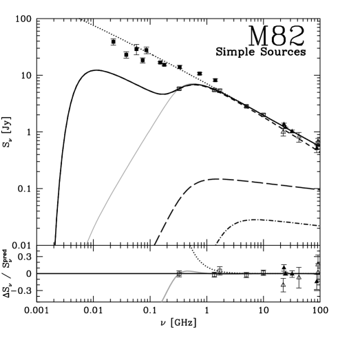
Figure 5: The effects of free-free absorption on M82’s radio spectrum. This is the best-fitting model to the Adebahr et al. (2012) and high-frequency data for H II regions surrounding simple sources. The total absorbed spectrum is shown as the black solid line. Its components are the synchrotron emission (short-dashed), free-free emission from absorbing H II regions (long-dashed), and free-free emission from dense non-absorbing H II regions (dash-dotted). The dotted line is the total emission if there were no absorption. I show a uniform slab fit to the $\geq 1\ \textrm{GHz}$ radio spectrum as the grey solid line. The residuals for the resolved data points are plotted on the bottom. The open squares are the Adebahr et al. (2012) data and the triangles are the high frequency data compiled in Williams & Bower (2010) (open for interferometric and filled for single-dish), while the filled squares are the low frequency unresolved observations in Table 1.

Figure 6: The effects of free-free absorption on M82’s radio spectrum, for H II regions surrounding a realistic stellar population. The line and point styles are the same as in Figure 5.

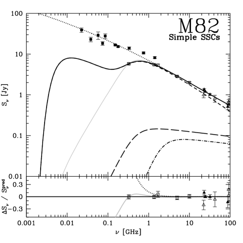
Figure 7: A model of the free-free absorption on M82’s radio spectrum, using the simple super star cluster assumptions described in section 2.3. The line and point styles are the same as in Figure 5.

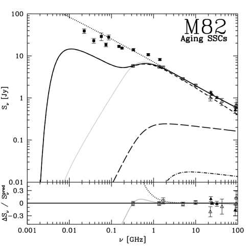
Figure 8: A model of the free-free absorption on M82’s radio spectrum, accounting for how the ionizing photon luminosity of SSCs evolve as they age. The line and point styles are the same as in Figure 5.

Effects on the spectrum shape – The effects of free-free absorption from discrete H II regions on the spectrum shape are concentrated within a finite frequency band. At high frequencies, the H II regions are transparent. At low frequencies, the H II regions are completely opaque, and $\alpha_{\rm eff}$ reaches some constant value; this changes the normalization of the spectrum, but not its intrinsic shape. These effects can be described more quantitatively in terms of the total spectral index $\tilde{\cal B}$ and spectral curvature $\tilde{\cal C}$:

$$\tilde{\cal B} \equiv \frac{d\log_{10}S_{\nu}^{\rm pred}}{d\log_{10}\nu}$$ (22)

$$\tilde{\cal C} \equiv \frac{d^{2}\log_{10}S_{\nu}^{\rm pred}}{d(\log_{10}\nu)^{2}};$$ (23)

these quantities differ from ${\cal B}$ and ${\cal C}$ in that they include free-free emission and absorption. I show how $\tilde{\cal B}$ and $\tilde{\cal C}$ vary with frequency in Figure 9 for the best-fitting models. Free-free absorption (the difference between black and grey lines) flattens the spectrum (higher $\tilde{\cal B}$) between $\sim 0.1-1\ \textrm{GHz}$: this is the regime where H II regions become optically thick. The resulting pulse in $\tilde{\cal B}$ is narrower when H II regions surround simple sources (dotted lines) instead of SSCs (dashed lines) or a realistic stellar population (solid line): in that model, the H II regions all have the same size, with the same turnover frequency, instead of the range of turnover frequencies for SSCs or a stellar population. In contrast, $\tilde{\cal B}$ plateaus at a value $\sim 1.6$ in the uniform slab model (dash-dotted line), as the free-free optical depth continues to rise. Finally, at frequencies below 20 MHz, the host galaxy’s WIM starts acting as a foreground screen to the starburst, and in all models $\tilde{\cal B}$ rises dramatically.

Likewise, there is a pulse in $\tilde{\cal C}$ that flips between negative (at low frequencies) and positive (at high frequencies) in the discrete H II absorption model. Free-free absorption in the uniform slab model, by contrast, causes a purely negative curvature. One obstacle for studies that measure intrinsic nonthermal curvature in the radio spectrum is that either free-free absorption or emission affects the spectrum at most observable radio frequencies. Only at frequencies of a few GHz does the intrinsic curvature dominate over that introduced by free-free absorption or emission. Even at low frequencies, where $\alpha_{\rm eff}$ is constant, the host galaxy WIM starts forcing the curvature to negative values.

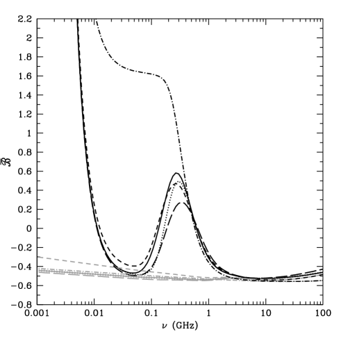
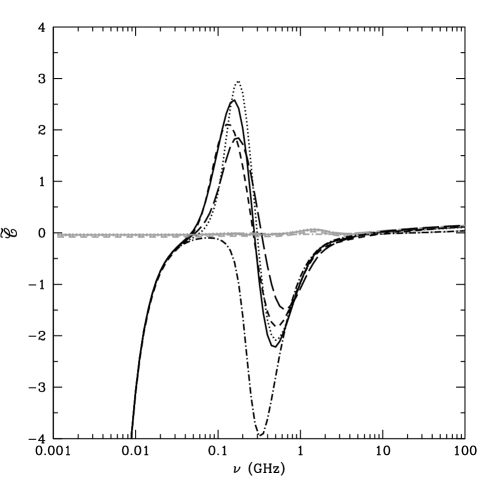
Figure 9: How free-free absorption affects the total spectral index $\tilde{\cal B}$ (left) and total spectral curvature $\tilde{\cal C}$ (right). I show these values with (black) and without (grey) free-free absorption. The line styles are for different best-fitting M82 models; dotted is simple sources, solid is for a stellar population, short-dashed is simple SSCs, long-dashed is aging SSCs, and dash-dotted is the uniform slab model. Free-free absorption introduces a pulse in the spectral index and curvature, as H II regions transition from being transparent to opaque with decreasing frequency.

The thermal pressure of H II regions – In my best-fitting discrete H II region models, the thermal pressure varies by a factor $\sim 3$, spanning the range $P_{\rm therm}/k=(2.5-7.5)\times 10^{6}\ \textrm{K}\ \textrm{cm}^{-3}$. Numerous studies have inferred the pressure of M82’s H II regions, using infrared and optical spectroscopy. Smith et al. (2006) found a fairly high pressure of $P_{\rm therm}/k=(1-2)\times 10^{7}\ \textrm{K}\ \textrm{cm}^{-3}$ for the H II region around the M82 A-1 super star cluster, several times greater than in my models. Note that M82 A-1 is relatively large ($\sim 10^{6}\ \textrm{M}_{\sun}$) compared to the small SSCs that would be expected to dominate the free-free absorption. Westmoquette et al. (2007) found lower pressures of $P_{\rm therm}/k=(5-10)\times 10^{6}\ \textrm{K}\ \textrm{cm}^{-3}$ in most M82 H II regions, comparable to those in my best-fitting models. Lord et al. (1996) inferred H II region pressures of $P_{\rm therm}/k=3\times 10^{6}\ \textrm{K}\ \textrm{cm}^{-3}$, based on infrared diagnostics of the surrounding denser and colder photodissociation regions. In any case, though, because of the range of densities I allowed for discrete H II regions, the pressures are necessarily higher than what I would find with a uniform slab model ($\sim 10^{6}\ \textrm{K}\ \textrm{cm}^{-3}$; compare with the similar results for NGC 253 in Carilli 1996).

Is free-free emission a good SFR indicator? – The low ionizing photon luminosities I derive are worrying, especially since I allow for ‘hidden’ free-free emission from compact H II regions that do not contribute to absorption. Even given the large errors and sparseness of the high frequency data, it seems difficult for there to be large amounts of free-free emission. On the other hand, thermal dust emission probably contributes to the highest frequency data points at some level, and there may be spinning dust emission as well, but including any dust emission would just tighten the constraints on the free-free emission.

It is possible, though, that the amount of free-free emission really is low in starburst galaxies – perhaps not a surprising hypothesis given that starbursts are dusty places that could readily absorb ionizing photons (c.f., Petrosian, Silk, & Field, 1972). Or, perhaps the problem is the opposite: ultraviolet photons could easily escape through the hot superwind phase that likely fills much of the starburst volume (e.g., Heckman et al., 1990), instead of ionizing the molecular gas. If so, then free-free emission is not necessarily a simple star-formation rate indicator in starbursts: its strength depends somehow on the radiative transfer in their dusty, multiphase environments, and it is buried even more than expected by synchrotron emission.

3.5 Useful Future Data

The need for high-resolution low frequency data is obvious. With current data, it is impossible to meaningfully favor the uniform slab model or the discrete H II region model on observational grounds. Aside from the single data point in Adebahr et al. (2012) and the maps of Basu et al. (2012), the low frequency data so vital in constraining free-free absorption comes from many instruments with varying but poor beam sizes. A future low frequency survey of M82 that resolves the starburst would ensure that flux from the surrounding galaxy is not making M82’s starburst appear brighter than it really is; such a survey can be done with the GMRT, VLA, or LOFAR.

Besides better low frequency data, it would be helpful to have high quality observations at 10 - 100 GHz. Then the flattening from free-free emission can be better constrained, if it is present. The Jansky VLA is able to observe at up to 50 GHz (Perley et al., 2011), and with its high sensitivity, it can measure the starburst spectrum with high accuracy. Moreover, as a single instrument, there would be fewer worries about systematics when comparing between data at different frequencies. Furthermore, it has high spatial resolution, so it can actually measure the characteristic sizes of H II regions, in particular searching for small, high density H II regions.

Another set of useful diagnostics comes from radio recombination lines, also observable with the Jansky VLA (Kepley et al., 2011). These constrain not only the ionizing photon luminosity of a starburst, but the densities and temperatures of the ionized gas. I note that Rodriguez-Rico et al. (2004) found, using H53$\alpha$ and H92$\alpha$ radio recombination lines, an ionizing photon luminosity of $1.6\times 10^{53}\ \textrm{s}^{-1}$ for M82. That is equivalent to a star-formation rate of $0.7\ \textrm{M}_{\sun}\ \textrm{yr}^{-1}$, compatible with the low ionizing photons I find here. On the other hand, Puxley et al. (1989) deduced an ionizing luminosity of $1.1\times 10^{54}\ \textrm{s}^{-1}$ also using the H53$\alpha$ line, which would correspond to a star-formation rate of $5\ \textrm{M}_{\sun}\ \textrm{yr}^{-1}$. This is significantly greater than what I find with my fits, but still a factor of $\sim 2$ lower than the infrared-derived star-formation rate. Future radio recombination line studies may clarify the situation.

4 Where do the radio spectra of starbursts really end?

My models of the radio spectrum are valid if the only relevant absorption processes are free-free absorption from the starburst H II regions, the host galaxy WIM, and the Galactic WIM. But the starburst radio spectrum cannot continue indefinitely to zero frequency, even ignoring the effects of the host galaxy and Milky Way WIM. The presence of volume-filling phases of ionized gas within starbursts ensures free-free absorption, as well as the Razin suppression of synchrotron emission. In addition, the purely nonthermal process of synchrotron self-absorption eventually must cut off the radio spectrum of starburst galaxies even if there is no diffuse ionized gas.

Aside from limiting the applicability of my models, these effects might inform us on different aspects of starburst environments. Free-free absorption from volume-filling ionized gas would probe the physical conditions in most of the starburst ISM. Detection of the synchrotron self-absorption or Razin effect would constrain starburst magnetic fields. They would also inform us of which ISM phase the synchrotron-emitting CR $e^{\pm}$ are in. In this section, I check whether these processes have any effects on starburst radio spectra at relevant frequencies.

4.1 Is there a WIM in starburst regions?

The conclusion that starbursts are partly transparent at low frequencies requires that there be no volume-filling warm ionized medium within the starburst region. Yet a WIM exists in the Milky Way and other normal star-forming galaxies, pervading at least 10% of the Galaxy out to a scale height of 1 kpc (the properties and theory of the WIM in normal galaxies is reviewed in Haffner et al. 2009). The Milky Way WIM becomes opaque at frequencies of a few MHz (Hoyle & Ellis, 1963; Alexander et al., 1969). While it is not fully certain how ionizing photons traverse such large distances in Milky Way, current theory is that not all ionizing photons are confined to dense H II regions but propagate into underdensities in the inhomogeneous ISM (e.g., Ciardi, Bianchi, & Ferrara 2002; Wood et al. 2010). Might a volume-filling WIM form in starburst regions in a similar way and account for the observed radio absorption?

There are several reasons to expect this is not the case, at least not within the starburst region proper. Firstly, other phases are expected to fill the starburst ISM, leaving little room for a WIM. A low density, hot plasma fill starbursts where supernova remnants do not experience strong radiative losses and the pressure is not extreme, simply because the supernova rate density is so great (e.g., Chevalier & Clegg, 1985; Heckman et al., 1990; Lord et al., 1996; Strickland & Heckman, 2007, 2009). Chandra has detected iron line emission consistent with the existence of this plasma in M82 (Strickland & Heckman, 2007, 2009). While ionized, this phase is so hot ($\sim 10^{8}\ \textrm{K}$) that there is essentially no free-free absorption (see section 4.3). Ionizing photons that escape into this phase propagate freely, but if the phase is volume-filling, they could easily escape the starburst entirely without ionizing neutral gas.

In the more extreme starbursts like those within Arp 220, the molecular medium with most of the gas mass is so dense that supernova remnants probably stall and the hot phase cannot form (e.g., Thornton et al. 1998; Thompson et al. 2005). Cold molecular gas likely fills most of these starburst regions. While the large neutral mass would become a formidable WIM if it were ionized, its sheer density poses a nearly insurmountable hurdle for a volume-filling homogeneous WIM. The neutral gas columns of starbursts are larger than those of the Milky Way by orders of magnitude. This means that the average optical depth of the neutral gas is hundreds, or thousands, of times larger than the Milky Way, with neutral gas and dust drastically limiting the range of ionizing photons.

The rapid recombination rate in the dense ISM is another obstacle for WIM formation. The maximum volume that can be ionized is equivalent to a Strömgren volume $Q_{\rm ion}/(n_{H}\alpha_{B})$. The maximum fraction of the starburst that can be ionized is:

$$f_{\rm fill}\leq 0.029\left(\frac{n_{H}}{1000\ \textrm{cm}^{-3}}\right)^{-2}\left(\frac{\rho_{\rm SFR}}{1000\ \textrm{M}_{\sun}\ \textrm{yr}^{-1}\ \textrm{kpc}^{-3}}\right).$$ (24)

at $T=10^{4}\ \textrm{K}$. I list the values for the specific examples of the Galactic Centre Central Molecular Zone (CMZ), M82, and Arp 220 in Table 3. In each case, only a few percent of the molecular gas can be ionized, suggesting the WIM is confined to small bubbles within the cold molecular medium.

Could we get around this limit by supposing that a volume-filled WIM has low density? The main problem is the surrounding ISM pressure, which is several orders of magnitude higher than in the Milky Way. If the WIM is supported by thermal pressure, its minimum hydrogen atom density at the known pressure of a starburst region is $n_{\rm min}\geq P_{\rm ISM}/(2kT)$. The large results are shown in Table 3. Then through equation 24, thermally-supported WIM makes up a small fraction of the starburst volume.

Table 3: Starburst WIM Constraints

Property	Galactic Centre CMZ	M82	Arp 220 Nuclei	References
${\rm SFR}$ ($\textrm{M}_{\sun}\ \textrm{yr}^{-1}$)	0.07	10	100	(1)
$R_{\rm SB}$ (pc)	112	250	100	(2)
$P_{\rm ISM}/k$ ($\textrm{K}\ \textrm{cm}^{-3}$)	$1.5\times 10^{6}$	$2\times 10^{7}$	$8\times 10^{9}$	(3)
$\Sigma_{\rm SFR}$ ($\textrm{M}_{\sun}\ \textrm{yr}^{-1}\ \textrm{kpc}^{-2}$)	2	50	3000	…
$\rho_{\rm SFR}$ ($\textrm{M}_{\sun}\ \textrm{yr}^{-1}\ \textrm{kpc}^{-3}$)	21	510	32000	(4)
WIM carved from mean density gas
$\langle n_{H}\rangle$ ($\textrm{cm}^{-3}$)	120	410	10000	(5)
$f_{\rm fill}$	$\leq 4.2\%$	$\leq 8.7\%$	$\leq 0.92\%$	…
Thermally supported WIM
$n_{\rm min}$ ($\textrm{cm}^{-3}$) a	$75$	$1000$	$400000$	…
$\nu_{\rm ff}^{\rm fill}$ (GHz) b	$\geq 0.59$	$\geq 12$	$\geq 3000$	…
$f_{\rm fill}$	$\leq 11\%$	$\leq 1.5\%$	$\geq 5.8\times 10^{-4}\%$	…
Turbulence-supported WIM ($\sigma=50\ \textrm{km}~{}\textrm{s}^{-1}$)
$n_{\rm min}$ ($\textrm{cm}^{-3}$) c	$8.8$	$120$	$46000$	…
$\langle n_{\rm min}\rangle_{V}$ ($\textrm{cm}^{-3}$) d	$2.3$	$37$	$15000$	…
$\nu_{\rm ff}^{\rm fill}$ (GHz) b	$\geq 0.022$	$\geq 0.43$	$\geq 110$	…
$f_{\rm fill}$	$\leq 800\%$	$\leq 110\%$	$\leq 0.043\%$	…

^a: Minimum hydrogen atom density ($P_{\rm ISM}/(2kT)$) needed to support the WIM thermally against the ISM pressure, for a temperature $T=10^{4}\ \textrm{K}$.

^b: If the starburst is completely filled with warm ionized gas with density $n_{\rm min}$ (for thermally supported WIM) or $\langle n_{\rm min}\rangle_{V}$ (for turbulently supported WIM), $\nu_{\rm ff}^{\rm fill}$ is the frequency at which the free-free absorption optical depth over $R_{\rm SB}$ is 1.

^c: Minimum hydrogen atom density ($2P_{\rm ISM}/(m_{H}\sigma^{2})$) needed to support the WIM turbulently against the ISM pressure.

^d: In a turbulently supported medium with average density $n_{\rm min}$ and Mach number ${\cal M}$, $\langle n_{\rm min}\rangle_{V}$ is the median density in the volume, $n_{\rm min}/\sqrt{1+{\cal M}^{2}}$. For the Mach number, I assume a temperature $10^{4}\ \textrm{K}$.

REFERENCES – (1) Yusef-Zadeh et al. (2009) and Crocker et al. (2011) for the Galactic Centre CMZ, from the IR luminosity Sanders et al. (2003) combined with the Kennicutt (1998) IR to SFR conversion for M82, and Downes & Solomon (1998) and Sakamoto et al. (2008) for Arp 220’s nuclei.

(2) Crocker et al. (2011) for the Galactic Centre CMZ, Goetz et al. (1990) and Williams & Bower (2010) for M82, and Sakamoto et al. (2008) for Arp 220’s nuclei.

(3) For the Galactic Centre CMZ, the listed value is a conservative estimate of the approximate magnetic and turbulent pressure from Figure 4 in Crocker et al. 2010. It is also roughly the thermal H II region pressure found by Zhao et al. (1993), and the Chevalier & Clegg (1985) superwind pressure for that $\Sigma_{\rm SFR}$. For M82, I use the hot superwind pressure from Strickland & Heckman (2007). For Arp 220’s radio nuclei, I take the turbulent energy density $\rho\sigma^{2}/2$, with $\sigma=100\ \textrm{km}~{}\textrm{s}^{-1}$ (Downes & Solomon, 1998).

(4) I use a scale height of 42 pc for the Galactic Centre CMZ (Crocker et al., 2011) and 50 pc for M82 and Arp 220’s nuclei.

(5) Crocker et al. (2011) for the Galactic Centre CMZ, Weiß et al. (2001) for M82, and Downes & Solomon (1998) for Arp 220’s nuclei.

There are two ways around these constraints. First, the WIM might be supported by supersonic turbulence. Then its density could be very small. Interestingly, Smith et al. (2006) infer a large turbulent pressure for the H II region around the M82 super star cluster A-1, so supersonic turbulence is not far-fetched. Furthermore, the Milky Way WIM is known to be transonic or weakly supersonic (Hill et al., 2008; Gaensler et al., 2011). But simulations show that large density inhomogeneities are a characteristic of mediums with supersonic turbulence. For a Mach number ${\cal M}$, half of the volume has a density of $\la\langle n_{H}\rangle/\sqrt{1+b^{2}{\cal M}^{2}}$, whereas half of the mass is in clumps with density $\ga\langle n_{H}\rangle\sqrt{1+b^{2}{\cal M}^{2}}$, where $b\approx 1/3$ – $1$ (Padoan, Nordlund, & Jones 1997; Ostriker, Stone, & Gamie 2001; I use a value of $b=1$ in this work). Thus the uniform slab model is still formally incorrect for the WIM.

While a volume-filling WIM of arbitrarily low densities can be supported as long as the turbulent velocities are high enough, there are interesting constraints if the turbulent speeds are similar to those in the molecular medium, roughly 50 $\textrm{km}~{}\textrm{s}^{-1}$. The first constraint the WIM faces is that it cannot be so dense that it free-free absorbs the $\geq\textrm{GHz}$ radio emission. In Table 3, I calculate the free-free turnover for a volume-filling WIM that is dense enough to be in pressure equilibrium with the surrounding material. For these results, I conservatively use the (rarefied) median density in the volume $\langle n_{\rm min}\rangle_{V}$. While the free-free turnovers are not yet constraining for the Galactic Centre CMZ or M82, a volume-filling WIM in Arp 220’s nuclei would cut off the radio emission below 110 GHz, in direct conflict with radio observations (Downes & Solomon, 1998). The other constraint is that $f_{\rm fill}$ cannot be much smaller than 1. Assuming the ionizing luminosity is given by equation 4, this is again not a problem for the Galactic Centre CMZ or M82. Note that the small amounts of free-free emission in M82 I found in section 3.4 indicate much smaller $f_{\rm fill}$. I find that $f_{\rm fill}$ can only be a fraction of a percent in Arp 220’s nuclei. Upping the turbulent WIM speed to $100\ \textrm{km}~{}\textrm{s}^{-1}$ in Arp 220, similar to the molecular gas turbulent speeds in that intense starburst, yields a lower average density ($\sim 13000\ \textrm{cm}^{-3}$) but does not relieve these two constraints. Much higher speeds would unbind the WIM entirely. In short, I conclude that while a volume-filling turbulent WIM is conceivable in M82 and weaker starbursts, it is very unlikely in the most extreme ULIRG starbursts like Arp 220.

Note at this point that the densities and pressures derived for the ‘WIM’ in Table 3 are similar to those known to hold in H II regions in starbursts. In the Milky Way and other normal galaxies, H II regions are overpressured, overdense regions that expand into the surrounding ISM, whereas the WIM has a pressure closer to equipartition with the rest of the ISM. But in starbursts, the H II regions themselves have densities and pressures comparable to the surrounding ISM. It is plausible that the H II regions are the WIM of starbursts.

In principle, another source of nonthermal pressure could also support the WIM. Magnetic fields are probably high in starbursts compared to the Milky Way (e.g., Thompson et al., 2006), but theory of the diffuse synchrotron emission indicates that they are either comparable to or weaker than turbulent pressure support (e.g., Lacki et al., 2010). CRs could also provide nonthermal pressure, but current theory suggests that they are either rapidly destroyed by radiative losses in starburst environments or blown away in starburst winds, preventing them from accumulating to pressures greater than the turbulent pressure (e.g., Lacki et al., 2010).

The other way around the pressure constraint is if the WIM is a transient feature far from pressure equilibrium. Starburst molecular media have turbulent Mach numbers of $\sim 100$, and thus have vast density contrasts. If $n_{H}\approx\langle n_{H}\rangle/100$ gas fills most of the volume of the molecular medium and becomes ionized, it forms a temporary coronal WIM. This ‘WIM’ would recombine within one eddy crossing time, but would be replenished as new material fills most of the volume. In Arp 220’s nuclei, a volume-filling, coronal WIM with a density $\sim 100\ \textrm{cm}^{-3}$ would become opaque at $\sim 750\ \textrm{MHz}$. The main question is whether the ionizing photons can actually reach all of the low density material. It is known that ionizing photons can travel further in turbulent media, by propagating in underdense regions, and it is thought that this is how ionizing photons escape through the Milky Way (e.g., Ciardi et al. 2002; Wood et al. 2010). However, the typical column depth through a turbulent medium is roughly the mean column depth (e.g., Ostriker et al., 2001), implying that ionizing photons would be stopped quickly in starbursts. Also note that theoretical models of the density distribution of turbulent gas assume isothermal gas, but ionized ‘voids’ would be much hotter, possibly invalidating those results. A study of these issues is worthwhile.

Finally, we can consider radio observations of starburst regions. The Galactic Centre CMZ is easily resolved, even at low frequency, and has been observed by the VLA at 74 MHz. The H II regions in the area and on the sightline are noticeable shadows on these images. Yet the radio synchrotron emission from this region still shines from behind the H II regions (Brogan et al., 2003; Nord et al., 2006). There appears to be no volume-filling WIM in the Galactic Centre region that is opaque at 74 MHz. Extragalactic starburst regions are much harder to resolve, but M82’s starburst has been resolved at 408 MHz with MERLIN (Wills et al., 1997). The free-free absorption visible in that image is concentrated in patches. Furthermore, some but not all of the supernova remnant radio spectra show signs of free-free absorption (Wills et al., 1997), which is consistent with clumpy ionizied gas.

4.2 The WIM in the starburst wind

While the starburst region proper may be clear of warm ionized matter, H$\alpha$ images of these galaxies depict spectacular eruptions of warm gas in the winds flowing out of the starburst. In the Chevalier & Clegg (1985) model of starburst winds, the pressure drops rapidly past the sonic point, located roughly at the boundary of the starburst region, so rarefied warm and cold material can survive beyond that radius. Warm gas could screen not only the starburst region, but the surrounding radio haloes of starbursts at low frequency.

We can estimate the mean density of the warm material by using the equation of continuity: $\langle n_{\rm warm}\rangle=\dot{M_{\rm warm}}/(m_{H}Av)$, where $A$ is the area of the wind. The mass outflow of the warm material can be parametrized with a mass-loading factor, $\beta_{\rm warm}=\dot{M_{\rm warm}}/{\rm SFR}$. While there are several models of starburst winds, they generally indicate that $\beta_{\rm warm}\approx 1$ (e.g., Strickland & Heckman, 2009; Murray et al., 2011). For example, Hopkins, Quataert, & Murray (2012) find a mass-loading factor of $\sim 3$ for M82-like starbursts, with roughly a third of that in warm material (Hopkins et al., 2013). The density of the warm material at $R_{\rm SB}$ is roughly

$$\langle n_{\rm warm}\rangle \approx\frac{\beta_{\rm warm}\Sigma_{\rm SFR}}{2vm_{H}}$$

$$\approx 3\beta_{\rm warm}\ \textrm{cm}^{-3}\left(\frac{\Sigma_{\rm SFR}}{50\ \textrm{M}_{\sun}\ \textrm{yr}^{-1}\ \textrm{kpc}^{-2}}\right)\left(\frac{v}{300\ \textrm{km}~{}\textrm{s}^{-1}}\right)^{-1}.$$ (25)

This is roughly the mean density that Shopbell & Bland-Hawthorn (1998) derive from H$\alpha$ observations of M82’s warm filaments. At distances beyond $R_{\rm SB}$, the mean density drops off as $r^{-2}$, and the free-free absorption coefficient drops rapidly as $r^{-4}$. Thus, the free-free optical depth for a face-on starburst is roughly $\alpha_{\rm H\ II}\times R_{\rm SB}$, and the turnover frequency is

$$\nu_{\rm ff} \approx 39\beta_{\rm warm}\ \textrm{MHz}\ \left(\frac{\Sigma_{\rm SFR}}{50\ \textrm{M}_{\sun}\ \textrm{yr}^{-1}\ \textrm{kpc}^{-2}}\right)\left(\frac{R_{\rm SB}}{250\ \textrm{pc}}\right)^{1/2}$$ (26)

$$\times\left(\frac{v}{300\ \textrm{km}~{}\textrm{s}^{-1}}\right)^{-1}\left(\frac{T}{10^{4}\ \textrm{K}}\right)^{-3/4}\left(\frac{\bar{g_{\rm ff}}}{10}\right)^{1/2}.$$

While not enough to interfere at 100 MHz in M82, the wind could pose a formidable screen for Arp 220, where it would be optically thick to $\sim 2\ \textrm{GHz}$ (Table 4).

Starburst winds have a biconical geometry, erupting out of the starburst midplane. It is not clear that this warm gas is actually along the line of sight along the midplane. Edge-on starbursts like M82 may not be screened by the warm material in the wind, then.

Yet the warm material in starburst winds is not volume-filling, but is strung on filaments, both in observed starbursts and in simulations (e.g., Cooper et al., 2008, 2009; Hopkins et al., 2013). The clumping would allow low frequency radio waves out on some sightlines, while blocking higher frequency waves on other sightlines, much like H II regions in the starburst region. However, the amount of clumping and its distribution is not well known. A calculation of the free-free absorption within the wind would be useful.

4.3 Free-free absorption in hot wind plasma

The high rate of supernovae in starburst galaxies occurring within a relatively small space is expected to excavate a hot phase of the ISM (McKee & Ostriker 1977; Heckman et al. 1990; Lord et al. 1996). The hot ISM erupts as a starburst-wide superwind, and is low density, but high in pressure, temperature, and, it is thought, filling factor (e.g., Chevalier & Clegg, 1985). Gas emitting in soft X-rays is indeed observed in many starbursts, though Strickland & Stevens (2000) argue that this emission comes from a cooler phase with lower filling factor than the actual wind. In addition, Chandra detected diffuse 6.7 keV iron line emission in M82 that supports the presence of $10^{8}\ \textrm{K}$ plasma (Strickland & Heckman, 2007).

Strickland & Heckman (2009) give the central density of the superwind from a thin disk as

$$n_{c} ={1.860\frac{\beta_{\rm hot}^{3/2}}{\epsilon_{\rm therm}^{1/2}}\frac{\dot{M}^{3/2}}{\dot{E}^{1/2}m_{H}(\pi R_{\rm SB}^{2})}}$$

$$={0.93\ \textrm{cm}^{-3}\left(\frac{\beta_{\rm hot}}{2}\right)^{3/2}\left(\frac{\epsilon_{\rm therm}}{0.75}\right)^{-1/2}\left(\frac{\Sigma_{\rm SFR}}{50\ \textrm{M}_{\sun}\ \textrm{yr}^{-1}\ \textrm{kpc}^{-2}}\right)}$$ (27)

and the central temperature for a completely ionized hydrogen wind as

$${T_{c}=\frac{0.2m_{H}\epsilon_{\rm therm}\dot{E}}{k\beta_{\rm hot}\dot{M}}=3.0\times 10^{7}\ \textrm{K}\left(\frac{\epsilon_{\rm therm}}{0.75}\right)\left(\frac{\beta}{2}\right)^{-1}.}$$ (28)

In these equations, $\epsilon_{\rm therm}\approx{0.75}$ is the fraction of supernova mechanical energy that ends up in thermal energy of the plasma, $\beta_{\rm hot}\approx 2$ is the mass-loading fraction (Strickland & Heckman, 2009).

I find that the high temperatures and low densities of starburst winds makes them extremely poor at free-free absorption. For $\bar{g_{\rm ff}}=20$, the turnover frequency is far below observability:

$$\nu_{\rm ff}\approx{24}\ \textrm{kHz}\ \left(\frac{\Sigma_{\rm SFR}}{50\ \textrm{M}_{\sun}\ \textrm{yr}^{-1}\ \textrm{kpc}^{-2}}\right)\left(\frac{s}{100\ \textrm{pc}}\right)^{1/2}.$$ (29)

I list these $\nu_{\rm ff}$ in Table 4 for representative starbursts. The starburst wind introduces free-free absorption only at frequencies less than $\sim 1$ – 2000 kHz, and is not important at the observable MHz radio frequencies fit by models.

4.4 Free-free absorption from cosmic ray-ionized molecular gas

Thompson et al. (2005) have argued that cold molecular gas, instead of rarefied supernova-heated material, fills most of the volume of starbursts. This could happen if supernova remnants rapidly lose their kinetic energy to radiative losses as they expand in a dense molecular medium, so that supernova-heated material fills only small isolated bubbles (Thornton et al., 1998). Then the molecular gas fills most of the starburst region, since the H II regions also have a small filling factor. Molecular gas is mostly neutral and dust extinction rapidly extinguishes any ultraviolet light (but see the caveats in section 4.1). However, cosmic rays should provide a relatively high level of ionization through fairly large columns (Suchkov, Allen, & Heckman 1993; Papadopoulos 2010), though the details of CR diffusion in starbursts and their penetration into molecular clouds is poorly understood.

As I argued in Lacki (2012), the CR ionization rate in starburst galaxies, where the proton spectrum is relatively hard, is

$$\zeta_{\rm CR} =\frac{\eta_{\rm ion}L_{\rm CR}m_{H}}{E_{\rm ion}M_{H}}$$ (30)

$${=1.8\times 10^{-15}\ \textrm{s}^{-1}\left(\frac{\rm\tau_{\rm gas}}{20\ \textrm{Myr}}\right)^{-1}\left(\frac{\eta_{\rm ion}}{0.1}\right).}$$ (31)

In this equation, $L_{\rm CR}$ is the luminosity of injected cosmic rays, $E_{\rm ion}\approx 30\ \textrm{eV}$ is the energy lost per cosmic ray ionization event (Cravens & Dalgarno, 1978), $M_{H}$ is the mass of gas in the galaxy, and $\eta_{\rm ion}\approx 0.1$ is the fraction of cosmic ray power that goes into ionization. In the Galactic Centre CMZ, winds probably remove CRs before they can ionize material, so $\eta_{\rm ion}$ is much lower than 0.1 (Crocker et al., 2011). The injected cosmic ray luminosity is thought to be approximately $10^{50}\ \textrm{erg}$ per supernova, and the supernova rate is $\Gamma_{\rm SN}=0.0064\ \textrm{yr}^{-1}({\rm SFR}/\textrm{M}_{\sun}\ \textrm{yr}^{-1})$, for a Salpeter IMF extending from 0.1 to $100\ \textrm{M}_{\sun}$. I have combined the SFR and $M_{H}$ into a single parameter $\tau_{\rm gas}\equiv M_{H}/{\rm SFR}$, which is about $\sim 20\ \textrm{Myr}$ in nuclear starbursts.

The ionization fraction is set by the ratio of the gas density $n_{H}$ and a characteristic density $n_{\rm ch}\approx 1000\ (\zeta_{\rm CR}/10^{-17}\ \textrm{s}^{-1})\ \textrm{cm}^{-3}$ from McKee (1989). In the cosmic ray ionized gas of starbursts, $n_{\rm ch}\gg n_{H}$ and $x_{e}\approx 10^{-7}(n_{\rm ch}/n_{H})$. Thus,

$$x_{e}\approx{10^{-5}\ \left(\frac{\zeta_{\rm CR}}{10^{-15}\ \textrm{s}}\right)\left(\frac{n_{H}}{1000\ \textrm{cm}^{-3}}\right)^{-1}}$$ (32)

While the ionization fraction is low, free-free absorption is enhanced by two factors: molecular material is dense, so the density of electrons and ions is relatively high, and molecular gas is cold. The electrons and ions reach thermal equilibrium with the surrounding gas long before they recombine (e.g., McCall et al., 2002). Assuming typical starburst molecular gas temperatures of $\sim 100\ \textrm{K}$ and that $n_{e}=n_{i}{=}x_{e}n_{H}$ and $\bar{g_{\rm ff}}=10$, the frequency of the free-free spectrum turnover is

$${\nu_{\rm ff}\approx 2.4\ \textrm{MHz}\ \left(\frac{\zeta_{\rm CR}}{10^{-15}\ \textrm{s}^{-1}}\right)\left(\frac{T}{100\ \textrm{K}}\right)^{-3/4}\left(\frac{s}{100\ \textrm{pc}}\right)^{1/2}}$$ (33)

Note that there is no density dependence, so inhomogeneities do not affect the free-free absorption turnover unless $\zeta_{\rm CR}$ itself varies.

4.5 The Razin effect

Free-free absorption is not the only process that cuts off the radio spectrum at low frequency. At low energies, the index of refraction of plasma suppresses the beaming of synchrotron radiation and causes it to fall off exponentially (Rybicki & Lightman, 1979). The frequency where this Razin effect becomes important is

$$\nu_{R}=185\ \textrm{kHz}\left(\frac{n_{e}}{1\ \textrm{cm}^{-3}}\right)\left(\frac{B}{100\ \mu\textrm{G}}\right)^{-1},$$ (34)

from Schlickeiser (2002).

Suppose all the gas in the starburst, both ionized and neutral, has the same magnetic field. $B$ and $\Sigma_{\rm SFR}$ are likely to depend on each other. The existence of the linear far-infrared radio correlation of galaxies constrains magnetic field strengths to be

$$B_{\rm FRC}\approx 470\ \mu\textrm{G}\left(\frac{\Sigma_{\rm SFR}}{50\ \textrm{M}_{\sun}\ \textrm{yr}^{-1}\ \textrm{kpc}^{-2}}\right)^{1/2}$$ (35)

from Lacki et al. (2010), after using the Kennicutt (1998) Schmidt law to convert between gas surface density and star-formation surface density. The Razin cutoff in the hot superwind of starbursts on the FIR-radio correlation is

$${\nu_{R}^{\rm hot}=37\ \textrm{kHz}\left(\frac{\Sigma_{\rm SFR}}{50\ \textrm{M}_{\sun}\ \textrm{yr}^{-1}\ \textrm{kpc}^{-2}}\right)^{1/2},}$$ (36)

varying between 5 and 500 kHz for starbursts with $\Sigma_{\rm SFR}$ between 1 and $10^{4}\ \textrm{M}_{\sun}\ \textrm{yr}^{-1}\ \textrm{kpc}^{-2}$. Table 4 lists the superwind Razin frequencies in a few other starburst regions.

If starbursts are instead filled with cosmic ray ionized gas, the low electron density ($n_{e}=x_{e}n_{H}$) of these regions imply even lower Razin cutoffs:

$${\nu_{R}^{\rm mol}=\displaystyle 0.39\ \textrm{kHz}\left(\frac{\zeta_{\rm CR}}{10^{-15}\ \textrm{s}^{-1}}\right)\left(\frac{\Sigma_{\rm SFR}}{50\ \textrm{M}_{\sun}\ \textrm{yr}^{-1}\ \textrm{kpc}^{-2}}\right)^{-1/2}}$$ (37)

In high density molecular regions, Zeeman splitting measurements indicate the magnetic field may be even higher (Robishaw, Quataert, & Heiles, 2008), so the Razin effect could be even less important.

Finally, in H II regions, which are fully ionized and high density:

$$\nu_{R}^{\rm HII}=\displaystyle 39\ \textrm{MHz}\ \left(\frac{n_{H}}{1000\ \textrm{cm}^{-3}}\right)\left(\frac{\Sigma_{\rm SFR}}{50\ \textrm{M}_{\sun}\ \textrm{yr}^{-1}\ \textrm{kpc}^{-2}}\right)^{-1/2}$$ (38)

Within these regions, we see that free-free absorption – which turns H II regions opaque at GHz frequencies – is more important than the Razin effect.

I conclude that the Razin effect is not observable in starburst galaxies.

4.6 Synchrotron self-absorption

Both free-free absorption and the Razin cutoff depend on the density distribution of ionized matter, something that is uncertain in starburst galaxies. However, because we observe synchrotron emission from starburst galaxies, there must also be synchrotron self-absorption in them as well.

The maximum brightness temperature of a synchrotron source is limited by synchrotron self-absorption to

$$T_{\rm max}\approx 3\times 10^{12}\ \textrm{K}\ \left(\frac{\nu}{\textrm{GHz}}\right)^{1/2}\left(\frac{B}{100\ \mu\textrm{G}}\right)^{-1/2}$$ (39)

from Begelman, Blandford, & Rees (1984). While the Razin effect can suppress synchrotron absorption (Crusius & Schlickeiser, 1988), I established it is not important for starbursts in section 4.5.

For resolved starbursts with an observed low frequency radio spectrum, it is possible to simply fit a model to the radio spectrum and see when, if ever, the brightness temperature $T_{b}$ is greater than $T_{\rm max}$. In general, though we expect starbursts to lie on the far-infrared radio correlation, with $\nu L_{\nu}(1\ \textrm{GHz})=10^{-6}L_{\rm TIR}=5630\ \textrm{L}_{\sun}({\rm SFR}/\textrm{M}_{\sun}\ \textrm{yr}^{-1})$ (Kennicutt 1998; Yun, Reddy, & Condon 2001). Ignoring geometrical factors, the starburst can be thought of as a sphere with radius $R_{\rm SB}$, so that the brightness temperature is $T_{b}=L_{\nu}c^{2}/(8\pi^{2}k\nu^{2}R_{\rm SB}^{2})$ in the Rayleigh-Jeans limit. Likewise, the star-formation surface density is $\Sigma_{\rm SFR}={\rm SFR}/(\pi R_{\rm SB}^{2})$. Putting all of these formulas together, I find that the FIR-radio correlation implies

$${T_{b}(1\ \textrm{GHz})\approx 30000\ \textrm{K}\left(\frac{\Sigma_{\rm SFR}}{50\ \textrm{M}_{\sun}\ \textrm{yr}^{-1}\ \textrm{kpc}^{-2}}\right).}$$ (40)

Now we need to extrapolate this down to low radio frequencies. The simplest assumption is that the radio spectral index is constant, and the brightness temperature has the form $T_{b}=T_{b}(1\ \textrm{GHz})(\nu/\textrm{GHz})^{-2.7}$. Then I can use eqn. 35 for $B$, and by equating eqns. 39 and 40, I find the synchrotron self-absorption turnover is at:

$${\nu_{\rm SSA}=2.4\ \textrm{MHz}\ \left(\frac{\Sigma_{\rm SFR}}{50\ \textrm{M}_{\sun}\ \textrm{yr}^{-1}\ \textrm{kpc}^{-2}}\right)^{0.39}.}$$ (41)

For starbursts on the FIR-radio correlation with $1\leq\Sigma_{\rm SFR}/(\textrm{M}_{\sun}\ \textrm{yr}^{-1}\ \textrm{kpc}^{-2})\leq 10^{4}$, $\nu_{\rm SSA}\approx 0.9-30\ \textrm{MHz}$. This result is conservative in the sense that the actual synchrotron self-absorption is weaker, because the radio spectra are free-free absorbed and tend to be flatter than $\nu^{-0.7}$. I list the approximate synchrotron self-absorption frequency of the Galactic Centre CMZ, M82’s starburst, and Arp 220’s radio nuclei in Table 4.

4.7 Summary

Table 4: Low frequency absorption in starbursts

Property	Galactic Centre CMZ	M82	Arp 220 Nuclei	References
${\rm SFR}$ ($\textrm{M}_{\sun}\ \textrm{yr}^{-1}$)	0.07	10	100	(1)
$R$ (pc)	112	250	100	(1)
$B$ ($\mu\textrm{G}$)	75	200	6000	(2)
$S_{\nu}(1.4\ \textrm{GHz})$ (Jy)	1915	5.5	$\sim 0.1$	(3)
$T_{b}(1.4\ \textrm{GHz})$ (K)	50	6000	340000	(4)
$\Sigma_{\rm SFR}$ ($\textrm{M}_{\sun}\ \textrm{yr}^{-1}\ \textrm{kpc}^{-2}$)	2	50	3000	…
$\langle n_{H}\rangle$ ($\textrm{cm}^{-3}$)	120	410	10000	(1)
$\nu_{\rm ff}$ (warm wind; MHz)	1.0	39	1500	…
$\nu_{\rm ff}$ (hot wind; MHz)	0.0010	0.038	1.5	…
$\nu_{\rm ff}$ (molecular; MHz)	$\ll 4$	$\la 4$	$\sim 4.3$	…
$\nu_{R}$ (hot wind; MHz)	0.0092	0.085	0.17	…
$\nu_{R}$ (molecular; MHz)	$\ll 5\times 10^{-4}$	$\la 7\times 10^{-4}$	$5.5\times 10^{-4}$	…
$\nu_{\rm SSA}$ (${\cal B}=-0.7$; $\Psi_{\rm SB}=1$; MHz)	0.68	3.4	19	…

References – (1) See Table 3.

(2) Crocker et al. (2011) for the Galactic Centre CMZ, de Cea del Pozo et al. (2009) and Persic et al. (2008) for M82, and Torres (2004) for Arp 220’s nuclei.

(3) Reich, Reich, & Fuerst (1990) (via Crocker et al. (2011)) for the Galactic Centre CMZ, Adebahr et al. (2012) for M82, and Downes & Solomon (1998) for Arp 220’s nuclei.

(4) I use distances of 8.0 kpc for the Galactic Centre, 3.6 Mpc for M82, and 80 Mpc for Arp 220.

Of the processes I considered, the most likely to suppress low frequency radio emission from starbursts is WIM in the starburst wind beyond the starburst region proper. This material is inhomogeneous, so its effects are unknown. I show that a volume-filling WIM is unlikely to exist within starburst regions themselves. Besides WIM in the starburst wind, the starburst’s H II regions dominate absorption down to $\sim 10\ \textrm{MHz}$. Internal processes within the starburst are generally unimportant, with a maximum cutoff frequency of $\sim 20\ \textrm{MHz}$ for synchrotron self-absorption in Arp 220-like starbursts. Free-free absorption from the volume-filling phases is unimportant down to a few MHz, as is the Razin effect.

5 Conclusions

With the renewed interest in low frequency radio astronomy, it is time for a better theoretical understanding of the low frequency radio spectra of starburst galaxies.

Previous models of the emission at these frequencies, if they considered free-free absorption at all, predicted that starbursts are opaque below a GHz. This was because they used the uniform slab model, assuming that ionized gas evenly pervaded the starburst. Most of the ionized gas mass is not truly diffuse in starbursts, but instead resides in discrete H II regions. If the H II regions are uniformly distributed throughout the starburst, they contribute to an effective absorption coefficient which should be used in the uniform slab formula. This coefficient does not approach infinity at low frequencies (Figures 1 – 4). If H II regions partially cover the starburst, they leave sightlines where the emission is unobscured. Furthermore, the H II regions are usually some way in from the surface of the starburst, so there is unobscured synchrotron emitting material on a sightline in front of the nearest H II region.

To demonstrate this method, I fit the radio spectrum of M82 with the effective absorption coefficient in the limit that the H II regions do not fill most of the starburst. The calculation ultimately reduces down to the density of the H II regions multiplied by the cross section of each to absorb background radio waves. I applied the calculations to the radio spectrum of M82. I find that models with discrete H II regions, around either individual OB stars or Super Star Clusters, are able to reproduce the radio spectrum reasonably well (see Figures 5–8).

The models I presented in the paper were relatively simple, assuming that H II regions are characterized by a single temperature and density. However, if the temperature and density distribution is known through other means, such as radio recombination lines, it is straightforward to integrate up the cross sections and calculate the effective absorption coefficient. A more important flaw in the approach described here is that I assume that H II regions are uniformly dense Strömgren spheres. However, dust absorption affects both the amount of ionizing photons available to produce H II regions (Petrosian et al., 1972), and the structure of H II regions (Draine, 2011b). Since my models suggest a low amount of free-free emission, which could mean that dust is absorbing ionizing photons, it is important that these effects be studied.

The other big factor that I have neglected is turbulence in H II regions, which is suggested by the observations of Smith et al. (2006). Supersonic turbulence introduces large density fluctuations, invalidating the assumption of uniform density within the Strömgren spheres. The molecular gas in starbursts is known to be highly supersonic (e.g., Downes & Solomon, 1998). Mellema et al. (2006) ran simulations of H II regions expanding through a turbulent ISM, finding the resulting H II regions are neither smooth nor uniformly ionized. A simulation of the free-free absorption from turbulent H II regions would be helpful, although there may be no easy formula for describing the radio absorption with a turbulent ISM.

This work implies that starbursts are in fact fairly bright at low frequencies. I considered whether any other absorption process could cause a turnover in the radio spectrum. While the are several factors inhibiting WIM growth in the starburst region proper, the warm gas in the starburst wind may prove to be a screen at low frequency, although those conclusions need to be verified. Internal processes within the starburst region – free-free absorption from the volume-filling gas phases, the Razin effect, and synchrotron self-absorption – are not important except below a few MHz. Thus, the free-free absorption from discrete H II regions is the essential ingredient for describing the radio spectrum at observable frequencies.

Note Added In Proof

Equation 4 is actually appropriate for a Salpeter IMF from 1 - 100 $M_{\odot}$, not 0.1 - 100 $M_{\odot}$ as stated in the text. This error affects the ‘Simple Sources’ and ‘Simple SSCs’ models, in Sections 2 and 3 and Figures 1 and 3. The values are right if all SFRs and stellar masses are assumed to include only stars with mass greater than 1 $M_{\odot}$. To convert $\alpha_{\rm eff}$ to 0.1 - 100 $M_{\odot}$, multiply it by 0.39. Likewise, the derived SFRs for these models of M82 can be divided by 0.39 to get the SFR between 0.1 and 100 $M_{\odot}$. The ‘Aging Clusters’ models were already converted to the correct IMF.

Appendix A A Method for Calculating Free-Free Absorption from Discrete H II Regions

A.1 Derivation of the effective absorption coefficient

I start by considering how a thin slice of the starburst with thickness $\Delta s$ absorbs background radio emission passing perpendicularly through it (Figure 10). The slice has an area $A$ and thickness large enough to contain a representative sample of the starburst’s H II regions, but otherwise can be small compared to the starburst. I am basically assuming that there is some scale smaller than the starburst size on which the number density (or distribution function) of H II regions is well-defined. I ignore the H II regions’ effects on radio emission emitted within the slice – as long as the slice is thin, and as long as the H II regions have a small filling factor, this should be a valid approximation. If the filling factor is large, a true uniform slab model is more accurate anyway.

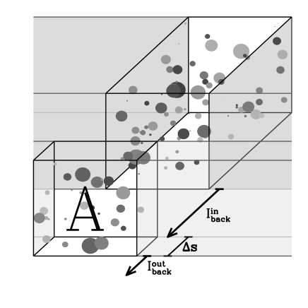
Figure 10: A sketch of how H II regions (filled circles) in a slice of the starburst with area $A$ and thickness $\Delta s$ absorb radiation from the column behind it. Different shades of grey in the H II regions can represent differing physical properties like electron density or temperature. The column can be small relative to the rest of the starburst (shaded in grey), but each slice is large enough to contain a representative sample of H II regions. A beam of light is emitted from the background column, enters perpendicular to the slice with intensity $I_{\rm back}^{\rm in}$ and emerges with intensity $I_{\rm back}^{\rm out}$, where $I$ is flux per solid angle. The fraction of light absorbed passing through the slice, which can be calculated by summing over individual H II regions in the slice, is directly related to the mean effective absorption coefficient of the starburst from H II regions. The coefficient then can be used in a uniform slab model (as suggested by the uniform grey shading of the rest of the starburst).

Suppose that there are $M$ H II regions (indexed by the number $m$). Each H II region passes a fraction $\Phi_{m}$ of the normal incident radiation $I_{\rm back}^{\rm in}A$ on the slice, where $I$ is flux per solid angle. For example, if a totally opaque sphere of radius $r$ sat in a slice of area $A$, $\Phi=1-(\pi r^{2}/A)$. Then the background radio intensity after passing through the slice is

$$I_{\rm back}^{\rm in}A\left[\prod_{m=1}^{M}\Phi_{m}\right]=I_{\rm back}^{\rm out}A.$$ (42)

Taking the logarithm of both sides, we can rephrase this as an optical depth:

$$-\sum_{m=1}^{M}\ln\Phi_{m}=-\ln\left(\frac{I_{\rm back}^{\rm out}}{I_{\rm back}^{\rm in}}\right)\equiv\Delta\tau_{\rm eff}.$$ (43)

Because each H II fraction only covers a small portion of the starburst, a convenient approximation is to define $\phi_{m}=1-\Phi_{m}$ and then to assume that $\ln\Phi_{m}\approx-\phi_{m}$. This is equivalent to saying that the H II regions do not overlap within the slice. Then we have

$$\sum_{m=1}^{M}\phi_{m}\approx\Delta\tau_{\rm eff}.$$ (44)

If there are $J$ types of H II regions, where each type of H II region absorbs the same amount of background radio, and if there are $K_{j}$ H II regions of each type $j$ within the slice, then

$$\Delta\tau_{\rm eff}\approx\sum_{j=1}^{J}K_{j}\phi_{j}.$$ (45)

More realistically, instead of having a few distinct types of H II regions, we might have a distribution function parametrizing the absorption properties of H II regions. Suppose the number of H II regions with some relevant physical quantity (such as radius) between $q$ and $q+dq$ and within a volume $dV$ is $dN/(dqdV)$. Then, since the volume of the slice is $A\Delta s$, the effective optical depth is

$$\Delta\tau_{\rm eff}\approx\int\frac{dN}{dqdV}A\Delta s\phi(q)dq.$$ (46)

Of course, this can easily be generalized to more than one parameter.

The effective optical depth across the slice translates to an effective absorption coefficient $\alpha_{\rm eff}\equiv\Delta\tau_{\rm eff}/(\Delta s)$ of the starburst. Furthermore, the quantity $A\phi(q)$ is an effective absorption cross section $\sigma$ for each H II region. So we have

$$\alpha_{\rm eff}\approx\int\frac{dN}{dqdV}\sigma(q)dq.$$

Therefore, the absorption coefficient reduces to a number density times a cross section, as might be expected.

If the density of H II regions is constant throughout the starburst, the equation of radiative transfer through the starburst, $dI/ds\approx-\alpha_{\rm eff}I+j$, has the uniform slab solution:

$$I=\frac{j}{\alpha_{\rm eff}}\left(1-e^{-\tau_{\rm eff}}\right)$$ (47)

except that the optical depth is the effective optical depth defined as $\tau_{\rm eff}=\alpha_{\rm eff}s$, where $s$ is the sightline length through the starburst. Of course, the density of H II regions may itself vary, for example, decreasing towards the edge of the starburst. However, the basic principle remains the same: the effective absorption coefficient is calculated at each point using equation 1, and then used in the radiative transfer equation to find the synchrotron intensity on each sightline.

A.2 The covering fraction

The calculation of the covering fraction of the H II regions is analogous to the calculation of the absorption of the radio flux. Essentially, we are interested in how much of the background sky is blocked by the H II regions. We can phrase this in terms of a flux calculation: if H II regions are totally opaque, the covering fraction is equal to the fraction of a uniform background intensity they absorb. Thus, we have for a distribution function of H II regions

$$\alpha_{\rm cover}=\int\frac{dN}{dqdV}\pi R_{S}^{2}dq$$ (48)

if each H II region is a sphere with radius $R_{S}$.

For the covering fraction calculation, the H II regions are treated as a foreground screen rather than as a uniform slab, as a H II region covers the background no matter how deep into the starburst it is. From the solution to absorption from a foreground screen, the probability any given sightline is covered is $P_{\rm cover}=1-e^{-\alpha_{\rm cover}s}$, where $s$ is the length of the sightline, assuming $\alpha_{\rm cover}$ is uniform throughout the starburst.

The length of a sightline may vary; for example, in an edge-on disc, it is shorter towards the rim than through the centre. The covering fraction for the entire starburst is the average of the covering probability $P_{\rm cover}$ over all sightlines that pass through the starburst:

$$f_{\rm cover}=\frac{1}{\Omega_{\rm obs}}\int(1-e^{-\alpha_{\rm cover}s})d\Omega_{\rm obs}.$$ (49)

In this equation, $\Omega_{\rm obs}$ is the solid angle subtended by the entire starburst from Earth. Note that since starbursts are small on the sky, $\Omega_{\rm obs}$ is directly proportional to the projected area of the starburst, $A_{\rm proj}$.

One consequence of $f_{\rm cover}<1$ is that we expect the optical depth to increase to some maximum value at low frequency and no further. If there are just a few H II regions, then the covering fraction is small and parts of the starburst remain completely unobscured. However, even if the density of H II regions is high, discrete H II regions tend to overlap from our point of view and cover each other instead of background material, causing $f_{\rm cover}$ to grow more slowly than $\tau_{\rm eff}$, and be slightly less than 1. In practice, the small filling factor of H II regions is the more important effect when $\tau_{\rm eff}\gg 1$ (see section A.3).

A.3 The filling fraction

Likewise, we can calculate the filling fraction for a distribution of Strömgren spheres. The starburst has a volume $V_{\rm SB}$, and a Strömgren sphere of radius $R_{S}$ has volume $4/3\pi R_{S}^{3}$. Therefore, each sphere leaves a fraction $1-4\pi R_{S}^{3}/(3V_{\rm SB})$ of the starburst unfilled, and the filling factor is

$$1-f_{\rm fill}\approx\exp\left[-\int\frac{dN}{dq}\left(\frac{4\pi R_{S}(q)^{3}}{3V_{\rm SB}}\right)dq\right].$$ (50)

When the filling factor is small, the spheres do not overlap, and

$$f_{\rm fill}\approx\int\frac{dN}{dq}\left(\frac{4\pi R_{S}(q)^{3}}{3V_{\rm SB}}\right)dq.$$ (51)

Since $R_{S}$ is much smaller than the size of the starburst, the filling factor of H II regions can be much smaller than 1 even if the covering fraction is nearly 1. As a result, a sightline through the starburst will not immediately intercept an H II region, even if the covering fraction is nearly 1. Instead, the first absorbing H II region on the sightline is buried past unobscured synchrotron-emitting space: this ensures that there is still synchrotron radio flux at low frequencies even if the covering fraction is high.

A.4 Limitations of the approach

While the approach I outlined above has more power than, for example, simply assuming all spheres are at the midplane and have the same radius, it still suffers some limits. First, the cross section depends on the structure of the H II regions. I assume that each H II regions is a uniformly dense sphere with radius $R_{S}$. Actual H II regions have more complex structures (e.g., Mellema et al., 2006).

On a more fundamental level, though, the approach assumes the H II regions have a well-defined number density, or local distribution function. But the relatively small numbers of H II regions per starburst introduces error. Some H II regions are too rare (for example, large SSCs), with perhaps one or two per starburst region, and formally invalidating the use of a local distribution function. As the considered volumes become smaller, stochastic effects become more important. The approach breaks down completely at small scales when there is fewer than $\sim 1$ H II region per volume.

To quantify this a bit, in the simple sources model (section 2.1) there are $\sim 22000$ H II regions per $1\ \textrm{M}_{\sun}\ \textrm{yr}^{-1}$ of star-formation. In M82, if ${\rm SFR}_{\rm eff}\approx 1\ \textrm{M}_{\sun}\ \textrm{yr}^{-1}$ (section 3.4), then there is about 1 H II region per $(10\ \textrm{pc})^{3}$, so the density is undefined on scales below $\sim 10\ \textrm{pc}$. Since I am considering the starburst as a whole, my approximation should work. There are fewer H II regions in the simple SSC model (section 2.3), 1300 per $1\ \textrm{M}_{\sun}\ \textrm{yr}^{-1}$ of star-formation for $M_{l}=1000\ \textrm{M}_{\sun}$, $M_{c}=5\times 10^{6}\ \textrm{M}_{\sun}$, and $t_{\rm ion}=10^{7}\ \textrm{yr}$. There are fewer SSCs of large mass: $dN/d\ln M_{\star}\approx 1300(M_{\star}/10^{3}\ \textrm{M}_{\sun})^{-1}({\rm SFR}_{\rm eff}/(\textrm{M}_{\sun}\textrm{yr}^{-1}))$. Thus, there is $\sim 1$ $M_{\star}\approx 10^{6}\ \textrm{M}_{\sun}$ SSCs in M82, and the absorption from these big H II regions is very poorly calculated. Fortunately, the $\sim 1000$ small SSCs are the source of most of the free-free absorption (see the discussion of clustering in section 2.3), so the assumption of a distribution function is sufficient for calculating the total absorption throughout the entire starburst.

None the less, there is need for a better quantification of stochastic effects.

Appendix B Summary of the radiative properties of Strömgren spheres

B.1 The effective cross section for translucent spheres

I treat H II regions as Strömgren spheres, which absorb the radiation behind them. The effective cross section of a sphere of radius $R_{S}$ and absorption coefficient $\alpha_{\rm HII}$ is equal to the projected area of the H II region times the fraction of background flux it obscures:

$$\sigma = \int_{0}^{R_{S}}2\pi y\left[1-e^{-2\alpha_{\rm HII}\sqrt{R_{S}^{2}-y^{2}}}\right]dy$$ (52)

$$= \pi R_{S}^{2}-\frac{\pi}{2\alpha_{\rm HII}^{2}}\left[1-e^{-2\alpha_{\rm HII}R_{S}}(1+2\alpha_{\rm HII}R_{S})\right]$$

When $\alpha_{\rm HII}$ is very large (at low frequency, for example), the spheres become totally opaque and the effective cross section is just $\pi R_{S}^{2}$. If instead $\alpha_{\rm HII}$ is very small, as at high frequency, the effective cross section goes as $V_{S}=(4/3)\pi\alpha_{\rm HII}R_{S}^{3}$.

Note that when all of the Strömgren spheres are optically thin, then $\alpha_{\rm eff}\approx f_{\rm fill}\alpha_{\rm HII}$. This is identical to the absorption coefficient in the uniform slab case when the electron density is equal to the volume-averaged electron density. Discrete H II region models diverge from the uniform slab solution only at low frequencies when H II regions start becoming opaque.

B.2 Luminosity of a translucent sphere

In order to calculate the free-free emission correctly, I must not only consider the absorption from the population of H II regions distributed throughout the starburst, but the free-free self-absorption within the H II region itself. For example, a very dense H II region may have a free-free absorption turnover at a few GHz, even if the starburst as a whole is transparent down to several hundred MHz.

The emergent free-free flux at a point on the surface of a uniform sphere is

$$F_{\nu}=2\pi B_{\nu}(T_{e})\int_{0}^{1}[1-e^{-2\alpha_{\nu}R_{S}\mu}]\mu d\mu,$$ (53)

where $\mu$ is the cosine of the angle between the centre of the sphere and a line of sight and $R_{S}$ is the radius of the sphere. The luminosity, which is the flux times the surface area, is

$$L_{\nu}=4\pi^{2}R_{S}^{2}B_{\nu}(T_{e})\left[1+\frac{1}{2\alpha_{\nu}^{2}R_{S}^{2}}(e^{-2\alpha_{\nu}R_{S}}(2\alpha_{\nu}R_{S}+1)-1)\right].$$ (54)

Appendix C Distribution of $Q_{\rm ion}^{\star}$ for a stellar population

To calculate the distribution function of $Q_{\rm ion}^{\star}$, I ran Starburst99 (version 6.0.4) models to find the number of each type of star in a stellar population (Leitherer et al., 1999). I considered a population formed with a continuous star-formation rate of $1.0\ \textrm{M}_{\sun}\ \textrm{yr}^{-1}$ over ages of 5 Myr and older. The IMF was assumed to be Salpeter ($dN/dM\propto M^{-2.35}$) over an interval $0.1\ \textrm{M}_{\sun}$ to $100\ \textrm{M}_{\sun}$. I assumed near Solar metallicity ($Z=0.02$). Table 5 lists the number of each type of ionizing star given these assumptions. Overall, I find that the number of stars of each type varies little for populations with ages over 10 Myr.

I took the ionizing photon luminosities of O and early B stars from Vacca, Garmany, & Shull (1996). As in Table 8 of Vacca et al. (1996), I group subgiants with dwarfs and bright giants with giants; in any case, $Q_{\rm ion}^{\star}$ varies slowly with luminosity class at a given spectral type. Vacca et al. (1996) does not give a $Q_{\rm ion}^{\star}$ for O3.5 stars, so I just take the average values of O3 and O4 stars.

For Wolf-Rayet stars, I note that in Smith, Norris, & Crowther (2002), late WN stars have $Q_{\rm ion}^{\star}\approx 10^{49.0}\ \textrm{s}^{-1}$, early WN stars have $Q_{\rm ion}^{\star}\approx 10^{49.3}\ \textrm{s}^{-1}$, late WC stars have $Q_{\rm ion}^{\star}\approx 10^{49.0}\ \textrm{s}^{-1}$, and early WC stars have $Q_{\rm ion}^{\star}\approx 10^{49.2}\ \textrm{s}^{-1}$. Finally, for WO stars, I just take $Q_{\rm ion}^{\star}\approx 10^{49.0}\ \textrm{s}^{-1}$; there are very few WO stars (about 1 in 10000 stars of all ionizing types), so the exact value should not affect results much. The ionizing luminosities are also listed in Table 5.

Table 5: Ionizing luminosities in a stellar population with a continuous SFR

Type	$\log_{10}(Q_{\rm ion}^{\star}/\textrm{s}^{-1})$ a	Number of stars b
		5 Myr	10 Myr	$\geq 15\ \textrm{Myr}$
O3.0 V+IV	49.87	27.81 + 27.65	27.81 + 27.65	27.81 + 27.65
O3.5 V+IV	49.79	69.70 + 27.89	69.70 + 27.89	69.70 + 27.89
O4.0 V+IV	49.70	89.49 + 17.83	90.07 + 17.83	90.07 + 17.83
O4.5 V+IV	49.61	119.9 + 50.22	120.1 + 50.22	120.1 + 50.22
O5.0 V+IV	49.53	167.9 + 69.52	167.9 + 69.52	167.9 + 69.52
O5.5 V+IV	49.43	213.5 + 92.90	213.5 + 92.90	213.5 + 92.90
O6.0 V+IV	49.34	296.4 + 78.71	296.4 + 78.71	296.4 + 78.71
O6.5 V+IV	49.23	384.8 + 124.8	384.8 + 124.8	384.8 + 124.8
O7.5 V+IV	49.00	534.4 + 114.8	534.4 + 114.8	534.4 + 114.8
O8.0 V+IV	48.87	672.2 + 200.0	672.2 + 200.0	672.2 + 200.0
O8.5 V+IV	48.72	969.8 + 268.2	995.7 + 320.6	995.7 + 320.6
O9.0 V+IV	48.56	1060 + 235.2	1261 + 408.0	1261 + 408.0
O9.5 V+IV	48.38	1139 + 237.3	1658 + 619.9	1658 + 619.9
B0.0 V+IV	48.16	1288 + 2.591	2568 + 546.7	2661 + 546.7
B0.5 V+IV	47.90	2650 + 0.000	4703 + 860.4	5516 + 866.6
O3.0 III+II	49.99	25.61 + 7.941	25.61 + 7.941	25.61 + 7.941
O3.5 III+II	49.92	7.300 + 8.495	7.300 + 8.495	7.300 + 8.495
O4.0 III+II	49.86	13.03 + 8.649	13.03 + 8.649	13.03 + 8.649
O4.5 III+II	49.80	22.84 + 12.22	22.84 + 12.22	22.84 + 12.22
O5.0 III+II	49.73	28.14 + 13.92	28.14 + 13.92	28.14 + 13.92
O5.5 III+II	49.65	29.29 + 19.56	29.30 + 19.56	29.30 + 19.56
O6.0 III+II	49.58	43.43 + 23.31	43.43 + 23.31	43.43 + 23.31
O6.5 III+II	49.50	51.97 + 32.81	51.97 + 32.82	51.97 + 32.82
O7.5 III+II	49.32	68.17 + 42.49	68.17 + 42.49	68.17 + 42.49
O8.0 III+II	49.22	84.84 + 52.96	84.84 + 52.96	84.84 + 52.96
O8.5 III+II	49.12	136.3 + 79.38	136.3 + 79.38	136.3 + 79.38
O9.0 III+II	48.97	140.6 + 79.29	194.5 + 79.29	194.5 + 79.29
O9.5 III+II	48.78	97.69 + 68.23	193.3 + 68.23	193.3 + 68.23
B0.0 III+II	48.55	0.000 + 70.95	217.6 + 98.38	217.6 + 98.38
B0.5 III+II	48.27	0.000 + 15.04	439.7 + 176.7	439.9 + 176.7
O3.0 I	50.11	236.6	236.6	236.6
O3.5 I	50.07	44.99	44.99	44.99
O4.0 I	50.02	41.35	41.35	41.35
O4.5 I	49.98	45.33	45.33	45.33
O5.0 I	49.93	45.19	45.19	45.19
O5.5 I	49.87	53.35	53.35	53.35
O6.0 I	49.81	42.80	42.80	42.80
O6.5 I	49.75	49.70	49.70	49.70
O7.5 I	49.62	59.38	59.38	59.38
O8.0 I	49.54	22.96	22.96	22.96
O8.5 I	49.45	43.62	43.64	43.64
O9.0 I	49.33	12.57	12.57	12.57
O9.5 I	49.17	39.45	39.45	39.45
WN Late	49.00	209.0	281.3	281.3
WN Early	49.30	175.4	177.7	177.7
WC Late	49.00	76.91	94.08	94.08
WC Early	49.20	59.43	61.22	61.22
WO	49.00	3.070	3.070	3.070

^a: Number of (hydrogen) ionizing photons emitted per star of the given type.

^b: Number of stars in a stellar population of the given age (5 Myr, 10 Myr, $\geq 15\ \textrm{Myr}$), if the star-formation rate has been constant. It is normalized to a star-formation rate of $1\ \textrm{M}_{\sun}\ \textrm{yr}^{-1}$. For dwarfs and subgiants, the entries are sums of the number of dwarfs and subgiants, respectively; likewise, the entries for giants and bright giants are sums of the number of giants and bright giants, respectively.

Appendix D Summary of the calculation of integrated flux from a starburst region

The uniform slab solution provides the intensity along a single sightline, which can be appropriate if the starburst is resolved. However, we often are interested in the integrated flux of the starburst. The sightline will have different lengths as it passes through different parts of the starburst. I summarize for the reader how much integrated flux remains after free-free absorption for three common geometries: a disc viewed face-on, a disc viewed edge-on, and a sphere.

D.1 A face-on disc

The flux observed at Earth is proportional to the luminosity emitted by the starburst into a unit solid angle, $dL/d\Omega_{\rm em}=\int IdA_{\rm proj}$. For a face-on disc of radius $R_{\rm SB}$ and midplane-to-edge height $h_{\rm SB}$ (edge-to-edge height $2h_{\rm SB}$), this is simply $dL/d\Omega_{\rm em}=\pi R_{\rm SB}^{2}I$, or

$$\frac{dL}{d\Omega_{\rm em}}=\pi R_{\rm SB}^{2}\frac{j}{\alpha_{\rm eff}}\left(1-e^{-2\alpha_{\rm eff}h_{\rm SB}}\right).$$ (55)

If the starburst had no absorption, it would have $dL/d\Omega_{\rm em}=2\pi R_{\rm SB}^{2}h_{\rm SB}j$. Therefore, the ratio of emergent flux to flux without absorption is

$$\Psi=\frac{1-e^{-2\alpha_{\rm eff}h_{\rm SB}}}{2\alpha_{\rm eff}h_{\rm SB}},$$ (56)

asymptoting to $1-\alpha_{\rm eff}h_{\rm SB}$ when $\alpha_{\rm eff}$ is very small and the starburst is nearly transparent.

The covering fraction for this geometry is just

$$f_{\rm cover}=1-e^{-2\alpha_{\rm cover}h_{\rm SB}}.$$ (57)

D.2 An edge-on disc

If the starburst disc is instead observed edge-on, the sightline length $s$ through the disc varies between 0 and $R_{\rm SB}$. Defining $y$ as the impact parameter from the centre of the disc, so that $y=\sqrt{R_{\rm SB}^{2}-s^{2}/4}$, the emergent flux is related to

$$\frac{dL}{d\Omega_{\rm em}} =4h_{\rm SB}\frac{j}{\alpha_{\rm eff}}\left(R_{\rm SB}-\int_{0}^{R_{\rm SB}}e^{-2\alpha_{\rm eff}\sqrt{R_{\rm SB}^{2}-y^{2}}}dy\right)$$

The ratio of emergent flux to flux without absorption is

$$\Psi=\frac{2}{\pi\alpha_{\rm eff}R_{\rm SB}}\left(1-\int_{0}^{1}e^{-2\alpha_{\rm eff}R_{\rm SB}\sqrt{1-u^{2}}}du\right).$$ (58)

When the disc is nearly transparent, with small $\alpha_{\rm eff}$, the ratio is approximately $1-8\alpha_{\rm eff}R_{\rm SB}/(3\pi)$.

The covering fraction is

$$f_{\rm cover}=1-\int_{0}^{1}e^{-2\alpha_{\rm cover}R_{\rm SB}\sqrt{1-u^{2}}}du.$$ (59)

When $\alpha_{\rm cover}R_{\rm SB}\ll 1$, $f_{\rm cover}\approx(\pi/2)R_{\rm SB}\alpha_{\rm cover}$.

D.3 A sphere

Suppose instead a starburst is a sphere with radius $R_{\rm SB}$. The emergent flux is now proportional to

$$\frac{dL}{d\Omega_{\rm em}} =\frac{\pi j}{\alpha_{\rm eff}}\left[R_{\rm SB}^{2}+\left(\frac{R_{\rm SB}}{\alpha_{\rm eff}}+\frac{1}{2\alpha_{\rm eff}^{2}}\right)e^{-2\alpha_{\rm eff}R_{\rm SB}}-\frac{1}{2\alpha_{\rm eff}^{2}}\right]$$ (60)

In a transparent sphere, the luminosity per solid angle is $dL/d\Omega_{\rm em}=(4/3)\pi R_{\rm SB}^{3}j$. Thus the ratio of emergent flux to unabsorbed flux is

$$\Psi=\frac{3}{4\alpha_{\rm eff}R_{\rm SB}^{3}}\left[R_{\rm SB}^{2}+\left(\frac{R_{\rm SB}}{\alpha_{\rm eff}}+\frac{1}{2\alpha_{\rm eff}^{2}}\right)e^{-2\alpha_{\rm eff}R_{\rm SB}}-\frac{1}{2\alpha_{\rm eff}^{2}}\right].$$ (61)

In the limit when $\alpha_{\rm eff}$ is small, this ratio is $1-(3/4)\alpha_{\rm eff}R_{\rm SB}$.

The covering fraction is

$$f_{\rm cover}=1+\frac{1}{2R_{\rm SB}^{2}\alpha_{\rm cover}^{2}}[e^{-2\alpha_{\rm cover}R_{\rm SB}}(2\alpha_{\rm cover}R_{\rm SB}+1)-1].$$ (62)

This reduces to $f_{\rm cover}\approx(4/3)\alpha_{\rm cover}R$ when $\alpha_{\rm cover}R_{\rm SB}\ll 1$.

References

- Adebahr et al. (2012) Adebahr, B., Krause, M., Klein, U., et al. 2012, arXiv:1209.5552
- Alexander et al. (1969) Alexander, J. K., Brown, L. W., Clark, T. A., Stone, R. G., & Weber, R. R. 1969, ApJL, 157, L163
- Anantharamaiah et al. (1993) Anantharamaiah, K. R., Zhao, J.-H., Goss, W. M., & Viallefond, F. 1993, ApJ, 419, 585
- Artyukh et al. (1969) Artyukh, V. S., Dagkesamanskii, V. V., Vitkevich, R. D., & Kozhukhov, V. N. 1969, Soviet Ast., 12, 567
- Baldwin et al. (1985) Baldwin, J. E., Boysen, R. C., Hales, S. E. G., Jennings, J. E., Waggett, P. C., Warner, P. J., Wilson, D. M. A. 1985, MNRAS, 217, 717
- Basu et al. (2012) Basu, A., Mitra, D., Wadadekar, Y., & Ishwara-Chandra, C. H. 2012, MNRAS, 419, 1136
- Begelman et al. (1984) Begelman, M. C., Blandford, R. D., & Rees, M. J. 1984, Reviews of Modern Physics, 56, 255
- Brogan et al. (2003) Brogan, C. L., Nord, M., Kassim, N., Lazio, J., & Anantharamaiah, K. 2003, Astronomische Nachrichten Supplement, 324, 17
- Carilli (1996) Carilli, C. L. 1996, A&A, 305, 402
- Chevalier & Clegg (1985) Chevalier, R. A., & Clegg, A. W. 1985, Nature, 317, 44
- Ciardi et al. (2002) Ciardi, B., Bianchi, S., & Ferrara, A. 2002, MNRAS, 331, 463
- Clemens et al. (2008) Clemens, M. S., Vega, O., Bressan, A., Granato, G. L., Silva, L., Panuzzo, P. 2008, A&A, 477, 95
- Clemens et al. (2010) Clemens, M. S., Scaife, A., Vega, O., & Bressan, A. 2010, MNRAS, 405, 887
- Cohen et al. (2007) Cohen, A. S., Lane, W. M., Cotton, W. D., Kassim, N. E., Lazio, T. J. W., Perley, R. A., Condon, J. J., Erickson, W. C. 2007, AJ, 134, 1245
- Condon et al. (1991) Condon, J. J., Huang, Z.-P., Yin, Q. F., & Thuan, T. X. 1991, ApJ, 378, 65
- Condon (1992) Condon, J. J. 1992, ARA&A, 30, 575
- Cooper et al. (2008) Cooper, J. L., Bicknell, G. V., Sutherland, R. S., & Bland-Hawthorn, J. 2008, ApJ, 674, 157
- Cooper et al. (2009) Cooper, J. L., Bicknell, G. V., Sutherland, R. S., & Bland-Hawthorn, J. 2009, ApJ, 703, 330
- Cravens & Dalgarno (1978) Cravens, T. E., & Dalgarno, A. 1978, ApJ, 219, 750
- Crocker et al. (2010) Crocker, R. M., Jones, D. I., Melia, F., Ott, J., & Protheroe, R. J. 2010, Nature, 463, 65
- Crocker et al. (2011) Crocker, R. M., Jones, D. I., Aharonian, F., Law, C. J., Melia, F., Oka, T., & Ott, J. 2011, MNRAS, 413, 763
- Crusius & Schlickeiser (1988) Crusius, A., & Schlickeiser, R. 1988, A&A, 196, 327
- de Cea del Pozo et al. (2009) de Cea del Pozo, E., Torres, D. F., & Rodriguez Marrero, A. Y. 2009, ApJ, 698, 1054
- Domingo-Santamaría & Torres (2005) Domingo-Santamaría, E. & Torres, D. F. 2005, A&A, 444, 403
- Downes & Solomon (1998) Downes, D., & Solomon, P. M. 1998, ApJ, 507, 615
- Draine (2011a) Draine, B. T. 2011a, Physics of the Interstellar and Intergalactic Medium (Princeton: Princeton University Press)
- Draine (2011b) Draine, B. T. 2011b, ApJ, 732, 100
- Ellingson et al. (2009) Ellingson, S. W., Clarke, T. E., Cohen, A., Craig, J., Kassim, N. E., Pihlstrom, Y., Rickard, L. J., Taylor, G. B. 2009, IEEE Proceedings, 97, 1421
- Fleishman & Tokarev (1995) Fleishman, G. D., & Tokarev, Y. V. 1995, A&A, 293, 565
- Förster Schreiber et al. (2003) Förster Schreiber, N. M., Genzel, R., Lutz, D., & Sternberg, A. 2003, ApJ, 599, 193
- Freedman & Madore (1988) Freedman, W. L., & Madore, B. F. 1988, ApJL, 332, L63
- Freedman et al. (1994) Freedman, W. L., et al. 1994, ApJ, 427, 628
- Gaensler et al. (2011) Gaensler, B. M., Haverkorn, M., Burkhart, B., et al. 2011, Nature, 478, 214
- Goetz et al. (1990) Goetz, M., Downes, D., Greve, A., & McKeith, C. D. 1990, A&A, 240, 52
- Haffner et al. (2009) Haffner, L. M., Dettmar, R.-J., Beckman, J. E., et al. 2009, Reviews of Modern Physics, 81, 969
- Hales et al. (1991) Hales, S. E. G., Mayer, C. J., Warner, P. J., & Baldwin, J. E. 1991, MNRAS, 251, 46
- Heckman et al. (1990) Heckman, T. M., Armus, L., & Miley, G. K. 1990, ApJS, 74, 833
- Hill et al. (2008) Hill, A. S., Benjamin, R. A., Kowal, G., Reynolds, R. J., Haffner, L. M., & Lazarian, A. 2008, ApJ, 686, 363
- Hopkins et al. (2012) Hopkins, P. F., Quataert, E., & Murray, N. 2012, MNRAS, 421, 3522
- Hopkins et al. (2013) Hopkins, P. F., Keres, D., Murray, N., et al. 2013, arXiv:1301.0841
- Hoyle & Ellis (1963) Hoyle, F., & Ellis, G. R. A. 1963, Australian Journal of Physics, 16, 1
- Hummel (1991) Hummel, E. 1991, A&A, 251, 442
- Israel & Mahoney (1990) Israel, F. P., & Mahoney, M. J. 1990, ApJ, 352, 30
- Kassim et al. (2007) Kassim, N. E., Lazio, T. J. W., Erickson, W. C., et al. 2007, ApJS, 172, 686
- Kellermann et al. (1969) Kellermann, K. I., Pauliny-Toth, I. I. K., & Williams, P. J. S. 1969, ApJ, 157, 1
- Kennicutt (1998) Kennicutt, R. C. 1998, ApJ, 498, 541
- Kepley et al. (2011) Kepley, A. A., Chomiuk, L., Johnson, K. E., Goss, W. M., Balser, D. S., Pisano, D. J. 2011, ApJL, 739, L24
- Klein et al. (1988) Klein, U., Wielebinski, R., & Morsi, H. W. 1988, A&A, 190, 41
- Lacki et al. (2010) Lacki, B. C., Thompson, T. A., & Quataert, E. 2010, ApJ, 717, 1
- Lacki (2012) Lacki, B. C. 2012, arXiv:1204.2580
- Laing & Peacock (1980) Laing, R. A., & Peacock, J. A. 1980, MNRAS, 190, 903
- Leitherer et al. (1999) Leitherer, C., Schaerer, D., Goldader, J. D., et al. 1999, ApJS, 123, 3
- Leroy et al. (2011) Leroy, A. K., Evans, A. S., Momjian, E., et al. 2011, ApJL, 739, L25
- Lord et al. (1996) Lord, S. D., Hollenbach, D. J., Haas, M. R., Rubin, R. H., Colgan, S. W. J., Erickson, E. F. 1996, ApJ, 465, 703
- Marvil et al. (2009) Marvil, J., Eilek, J., & Owen, F. 2009, Bulletin of the American Astronomical Society, 41, #418.02
- McCall et al. (2002) McCall, B. J., Hinkle, K. H., Geballe, T. R., et al. 2002, ApJ, 567, 391
- McCrady & Graham (2007) McCrady, N., & Graham, J. R. 2007, ApJ, 663, 844
- McDonald et al. (2002) McDonald, A. R., Muxlow, T. W. B., Wills, K. A., Pedlar, A., & Beswick, R. J. 2002, MNRAS, 334, 912
- McKee & Ostriker (1977) McKee, C. F., & Ostriker, J. P. 1977, ApJ, 218, 148
- McKee (1989) McKee, C. F. 1989, ApJ, 345, 782
- Mellema et al. (2006) Mellema, G., Arthur, S. J., Henney, W. J., Iliev, I. T., & Shapiro, P. R. 2006, ApJ, 647, 397
- Melo et al. (2005) Melo, V. P., Muñoz-Tuñón, C., Maíz-Apellániz, J., & Tenorio-Tagle, G. 2005, ApJ, 619, 270
- Meurer et al. (1995) Meurer, G. R., Heckman, T. M., Leitherer, C., Kinney, A., Robert, C., Garnett, D. R. 1995, AJ, 110, 2665
- Murphy (2009) Murphy, E. J. 2009, ApJ, 706, 482
- Murphy et al. (2011) Murphy, E. J., Condon, J. J., Schinnerer, E., et al. 2011, ApJ, 737, 67
- Murray et al. (2011) Murray, N., Ménard, B., & Thompson, T. A. 2011, ApJ, 735, 66
- Niklas et al. (1997) Niklas, S., Klein, U., & Wielebinski, R. 1997, A&A, 322, 19
- Nord et al. (2006) Nord, M. E., Henning, P. A., Rand, R. J., Lazio, T. J. W., & Kassim, N. E. 2006, AJ, 132, 242
- O’Connell et al. (1995) O’Connell, R. W., Gallagher, J. S., III, Hunter, D. A., & Colley, W. N. 1995, ApJL, 446, L1
- Ostriker et al. (2001) Ostriker, E. C., Stone, J. M., & Gammie, C. F. 2001, ApJ, 546, 980
- Padoan et al. (1997) Padoan, P., Nordlund, A., & Jones, B. J. T. 1997, MNRAS, 288, 145
- Papadopoulos (2010) Papadopoulos, P. P. 2010, ApJ, 720, 226
- Perley et al. (2011) Perley, R. A., Chandler, C. J., Butler, B. J., & Wrobel, J. M. 2011, ApJL, 739, L1
- Persic et al. (2008) Persic, M., Rephaeli, Y., & Arieli, Y. 2008, A&A, 486, 143
- Peterson & Webber (2002) Peterson, J. D., & Webber, W. R. 2002, ApJ, 575, 217
- Petrosian et al. (1972) Petrosian, V., Silk, J., & Field, G. B. 1972, ApJL, 177, L69
- Puxley et al. (1989) Puxley, P. J., Brand, P. W. J. L., Moore, T. J. T., Mountain, C. M., Nakai, N., Yamashita, T. 1989, ApJ, 345, 163
- Reich et al. (1990) Reich, W., Reich, P., & Fuerst, E. 1990, A&AS, 83, 539
- Rengarajan (2005) Rengarajan, T. N. 2005, Proc. 29th Int. Cosmic Ray Conf. (Pune), 3.
- Rephaeli et al. (2010) Rephaeli, Y., Arieli, Y., & Persic, M. 2010, MNRAS, 401, 473
- Robishaw et al. (2008) Robishaw, T., Quataert, E., & Heiles, C. 2008, ApJ, 680, 981
- Rodriguez-Rico et al. (2004) Rodriguez-Rico, C. A., Viallefond, F., Zhao, J.-H., Goss, W. M., & Anantharamaiah, K. R. 2004, ApJ, 616, 783
- Rodríguez-Rico et al. (2005) Rodríguez-Rico, C. A., Goss, W. M., Viallefond, F., Zhao, J.-H., Gómez, Y., Anantharamaiah, K. R. 2005, ApJ, 633, 198
- Roger et al. (1986) Roger, R. S., Costain, C. H., & Stewart, D. I. 1986, A&AS, 65, 485
- Rybicki & Lightman (1979) Rybicki, G. B. & Lightman, A. P. 1979, Radiative Processes in Astrophysics, (New York: Wiley-VCH)
- Sakai & Madore (1999) Sakai, S., & Madore, B. F. 1999, ApJ, 526, 599
- Sakamoto et al. (2008) Sakamoto, K., et al. 2008, ApJ, 684, 957
- Sanders et al. (2003) Sanders, D. B., Mazzarella, J. M., Kim, D.-C., Surace, J. A., & Soifer, B. T. 2003, AJ, 126, 1607
- Schlickeiser (2002) Schlickeiser, R. 2002, Cosmic Ray Astrophysics, (New York: Springer).
- Shopbell & Bland-Hawthorn (1998) Shopbell, P. L., & Bland-Hawthorn, J. 1998, ApJ, 493, 129
- Smith et al. (2002) Smith, L. J., Norris, R. P. F., & Crowther, P. A. 2002, MNRAS, 337, 1309
- Smith et al. (2006) Smith, L. J., Westmoquette, M. S., Gallagher, J. S., O’Connell, R. W., Rosario, D. J., de Grijs, R. 2006, MNRAS, 370, 513
- Sopp & Alexander (1989) Sopp, H. M., & Alexander, P. 1989, ApSS, 157, 287
- Sopp & Alexander (1991) Sopp, H. M., & Alexander, P. 1991, MNRAS, 251, 112
- Strickland & Stevens (2000) Strickland, D. K., & Stevens, I. R. 2000, MNRAS, 314, 511